Sampled-Data Control Based Consensus of Fractional-Order Multi-Agent Systems

Abstract

In this paper, we investigate consensus control of fractional-order multi-agent systems with order in $(0,1)$ via sampled-data control. A new scheme to design distributed controllers with rigorous analysis is presented by utilizing the unique properties of fractional-order calculus, namely hereditary and infinite memory. It is established that global boundedness of all closed-loop signals is ensured and asymptotic consensus is realized. Simulation studies are conducted to illustrate the effectiveness of the proposed control method and verify the obtained results.

Keywords Fractional-order; sampled-data control; multi-agent systems; consensus.

1 Introduction

Multi-agent systems are widely studied in the past decades because of their applications in various areas such as formation control, distributed sensor network, and so on [1, 2, 3]. Generally, the target of distributed consensus control is to achieve an agreement for the states of all the systems connected in a network by designing a suitable controller for each agent depending on locally available information from itself and its neighbors.

Recently, consensus control problems for integer-order multi-agent systems have been broadly investigated, see for examples [4, 5, 6, 7, 8, 9, 10, 11, 12], and references therein. As for the consensus control problem of fractional-order multi-agent systems, it is first studied in [13], where the conditions for achieving consensus in term of network structure and the number of agents are provided. In [14], where an undirected graph is considered, a consensus protocol with switching order is raised to increase convergence speed. Consensus involving communication delays is addressed in [15]. Observer-based leader-following consensus problem is investigated in [16], where the leader is described as a second-order integer model while the followers are fractional-order systems with order $\alpha\in(0,2)$. Consensus for incommensurate nonlinear fractional-order multi-agent systems with system uncertainties and external disturbances is addressed in [17].

All the works above are studied with continuous control, which requires control signals to be updated and transmitted continuously. In comparison with continuous control, sampled-data control for continuous-time systems, which can be found in for example [18] and [19], possesses various of benefits such as low cost and be more practical in implementation. Many research works for integer-order multi-agent systems with sampled-data control have also been done and a survey on this topic is provided in [20]. However, results on sampled-data control of fractional-order multi-agent systems are still limited. The consensus problem of such systems with directed graph via sampled-data control is investigated in [21, 22, 23]. In [24], consensus of linear fractional-order multi-agent systems over a communication topology, whose coupling structure is not necessary to be Laplacian, is studied. Event-triggering sampled-data control of fractional-order multi-agent systems is proposed in [25], in which the networked graph for the agents is assumed to be undirected.

From the definitions of fractional integral and derivative reviewed in Section 2, it can be observed that they can both be treated as weighted integral, which reveals the properties of fractional-order calculus: hereditary and infinite memory. Due to these unique properties, the initial values and the “history" of the variables in the entire interval of integration play extremely important roles in solving fractional-order equations. It is noted that such properties are not considered in the existing literature on sampled-data control of fractional-order multi-agent systems mentioned above. Instead, by dividing the entire time history to sampling intervals, the solutions of fractional-order equations at the beginning of each sampling interval are used as the new initial values for this sampling interval. As a result, the closed-loop fractional-order systems obtained are transformed to discrete-time systems, where the evolutions of step-forward states only rely on the current states and control inputs. However, when taking these properties into account, the evolutions should also depend on the previous states at all the discrete-time sampling instants starting from the initial time $t_{0}$.

Motivated by the discussions above, we address the consensus issue with the consideration of such unique characteristics of fractional-order calculus. With our proposed control design scheme, it is shown that the closed-loop system is globally stable and asymptotic consensus for fractional-order multi-agent systems is achieved. Different from existing research works, the resulting fractional-order system is rigorously analyzed by considering time evolution of the system states which depends on their initial values at $t_{0}$ and also all the previous control signals. A new challenge that is to establish the global boundedness of the proposed distributed controllers which contain all the previous control inputs is overcome in this paper. Simulation studies illustrate the effectiveness of the proposed control scheme and also reveal its accuracy on achieving asymptotic consensus compared to an existing approach.

The rest of the paper is organized as follows. Preliminaries are provided and the class of fractional-order multi-agent systems considered is described in Section 2. In Section 3, the design of distributed controllers is presented in detail with analysis. In Section 4, the scheme is illustrated by simulation studies with comparison to that in [21]. Finally the paper is concluded in Section 5.

2 Preliminaries and Problem Formulation

2.1 Preliminaries

Definition 1 [26]: The fractional integral of an integrable function $f(t)$ with $\alpha\in\mathbb{R}^{+}$ and initial time $t_{0}$ is

$${}_{t_{0}}\!{\mathit{I}}_{t}^{\alpha}f(t)=\frac{1}{\Gamma(\alpha)}\int_{t_{0}}^{t}\frac{f(\tau)}{(t-\tau)^{1-\alpha}}\,d\tau$$ (1)

where $\Gamma(\cdot)$ denotes the well-known Gamma function, which is defined as $\Gamma(z)=\int_{0}^{\infty}e^{-t}t^{z-1}\,dt$, where $z\in\mathbb{C}$. One of the significant properties of Gamma function is [27]: $\Gamma(z+1)=z\Gamma(z),\,\Gamma(n+1)=n\Gamma(n)=n(n-1)\Gamma(n-1)=\cdots=n!,\,\Gamma(-n)=\infty$, where $n\in\mathbb{N}_{0}=\{n|n\geq 0,n\in\mathbb{N}\}$.

Definition 2 [26]: The Caputo fractional derivative of a function is defined as

$${}_{t_{0}}^{C}\!{\mathcal{D}}_{t}^{\alpha}f(t) ={}_{t_{0}}{\mathit{I}}_{t}^{(m-\alpha)}\frac{\mathrm{d}^{m}}{\mathrm{d}t^{m}}f(t)$$ (2)

$$=\frac{1}{\Gamma(m-\alpha)}\int_{t_{0}}^{t}\frac{f^{(m)}(\tau)}{(t-\tau)^{\alpha-m+1}}\,d\tau$$

where $m-1<\alpha<m\in\mathbb{Z}^{+}$. From (2) we can observe that the Caputo derivative of a constant is $0$. Another commonly used fractional derivative is named Riemann-Liouville (RL) and the RL fractional derivative of a function $f(t)$ is denoted as ${}_{t_{0}}^{RL}\!{\mathcal{D}}_{t}^{\alpha}f(t)$. Different from the Caputo derivative, RL derivative of a constant is not equal to $0$ [28, 26].

The initial values are needed in order to obtain the unique solution for fractional differential equation ${}_{t_{0}}\!{\mathcal{D}}_{t}^{\alpha}x(t)=f(x,t)$, ($m-1<\alpha<m\in\mathbb{Z}^{+}$ and $t\geq t_{0}$). According to [29, 26] and [30], fractional differential equations with Caputo-type derivative have initial values that are in-line with integer-order differential equations, i.e. $x(t_{0}),x^{\prime}(t_{0}),\dots,x^{(m-1)}(t_{0})$, which contain specific physical interpretations. Therefore, Caputo-type fractional systems are frequently employed in practical analysis.

Definition 3 [31, 32, 33]: For fractional nonautonomous system ${}_{t_{0}}\!{\mathcal{D}}_{t}^{\alpha}x_{i}(t)=f_{i}(x,t)$ ($i=1,2,\dots,n$), where $0<\alpha<1$, initial condition $x(t_{0})=[x_{1}(t_{0}),x_{2}(t_{0}),\dots,x_{n}(t_{0})]^{\mathrm{T}}\in\mathbb{R}^{n}$, $f_{i}(x,t):[t_{0},\infty)\times\Omega\rightarrow\mathbb{R}^{n}$ is locally Lipschitz in $x$ and piecewise continuous in $t$ (which insinuates the existence and uniqueness of the solution to the fractional systems [26]), ${}_{t_{0}}\!{\mathcal{D}}_{t}^{\alpha}$ denotes Caputo or RL fractional derivative and $\Omega\in\mathbb{R}^{n}$ stands for a region that contains the origin $x=[0,0,\dots,0]^{\mathrm{T}}$, the equilibrium $x^{*}=[x_{1}^{*},x_{2}^{*},\dots,x_{n}^{*}]^{\mathrm{T}}$ of this system is defined as ${}_{t_{0}}\!{\mathcal{D}}_{t}^{\alpha}x^{*}=f_{i}(x^{*},t)$ for $t\geq t_{0}$.

Lemma 1 [28]: If $x(t)\in\mathbb{R}^{n}$ satisfies

$${}_{t_{0}}^{C}\!{\mathcal{D}}_{t}^{\alpha}x(t) =f(x,t),\;x(t_{0})=x_{0},$$ (3)

where $0<\alpha<1$ and $f(x,t)\in L_{1}[t_{0},T]$, then it also satisfies the Volterra fractional integral

$$x(t)=x_{0}+\frac{1}{\Gamma(\alpha)}\int_{t_{0}}^{t}(t-\tau)^{\alpha-1}f\big{(}x(\tau),\tau\big{)}d\tau,$$ (4)

with $t_{0}\leq t\leq T$ and vice versa.

Lemma 2: For $\forall j\in\mathbb{Z}^{+}$ and $0<\alpha<1$, the following results hold
1) $0<\lvert(j+1)^{\alpha}-2j^{\alpha}+(j-1)^{\alpha}\rvert<1$,
2) $\lim_{j\rightarrow\infty}\lvert(j+1)^{\alpha}-2j^{\alpha}+(j-1)^{\alpha}\rvert=0$.

Proof: Define

$$f(j)=(j+1)^{\alpha}-2j^{\alpha}+(j-1)^{\alpha}$$ (5)

and

$$g(s) =s^{\alpha}-(s-1)^{\alpha}.$$ (6)

It can be shown from (6) that, for $\forall s\in\mathbb{R}^{+}$,

$$g(s) >0,$$ (7)

$$\frac{dg(s)}{ds}=\alpha s^{\alpha-1} -\alpha(s-1)^{\alpha-1}<0.$$

From (7), we can obtain that $g(s)$ is monotonically decreasing and $\lim_{s\rightarrow\infty}g(s)=0$, which further implies that $f(j)<0$ and will monotonically tends to 0 as $j$ tends to $\infty$. Additionally, it can be easily checked that $\lvert f(1)\rvert<1$ for $0<\alpha<1$. This complete the proof.

2.2 Problem Formulation

In this paper, Caputo-type definition of the fractional derivatives is utilized. A group of $\mathit{N}$ fractional-order agents are governed by

$${}_{t_{0}}^{C}\!{\mathcal{D}}_{t}^{\alpha} x_{i}(t)=u_{i}(t),\text{ for }i=1,2,\cdots,N$$ (8)

where the fractional-orders of all the states are equal to $\alpha\in(0,1)$, $x_{i}\in\mathbb{R}$ and $u_{i}\in\mathbb{R}$ represent the measurable state and control input of $i$-th agent, respectively.

Remark 1: All the agents in this paper are in one-dimensional space for convenience. The results established can be easily extended to $n$-dimensional space by applying the Kronecker product.

In this paper, the control problem is to design distributed controller $u_{i}$ for each agent described in (8) to achieve the following objectives: 1) all the signals in the closed-loop systems are globally bounded; 2) asymptotic consensus for fractional-order systems (8) is ensured, i.e. $\lim_{t\rightarrow\infty}\lVert x_{i}(t)-x_{j}(t)\rVert=0,\,\forall i,j=1,2,\cdots,\mathit{N}$, and additionally, $\lim_{{t\rightarrow\infty}}x_{i}(t)=\frac{\sum_{i=1}^{N}x_{i}(t_{0})}{N}$.

Suppose that the communications among the $\mathit{N}$ agents can be represented by a directed graph $\mathcal{G}\triangleq(\mathcal{V},\mathcal{E})$ where $\mathcal{V}=\{1,2,\cdots,\mathit{N}\}$ means the set of indexes (or vertices) corresponding to each agent, $\mathcal{E}\subseteq\mathcal{V}\times\mathcal{V}$ is the set of edges between two distinct agents. An edge $(i,j)\in\mathcal{E}$ denotes that agent $j$ can obtain information from agent $i$, but not necessarily vice versa. In this case, agent $i$ is called a neighbor of agent $j$ and we indicate the set of neighbors for agent $i$ as $\mathcal{N}_{i}$. In this paper, $(i,i)\notin\mathcal{E}$ and $i\notin\mathcal{N}_{i}$ since self edges $(i,i)$ are not allowed. $\mathit{A}=[a_{ij}]\in\mathbb{R}^{N\times N}$ is the connectivity matrix with $a_{ij}=1$ if $(j,i)\in\mathcal{E}$ and $a_{ij}=0$ if $(j,i)\notin\mathcal{E}$ defined. Throughout this paper, the diagonal elements $a_{ii}=0$. An in-degree matrix $\triangle$ is introduced as $\triangle=\text{diag}(\triangle_{i})\in\mathbb{R}^{N\times N}$ with $\triangle_{i}=\sum_{j\in\mathcal{N}_{i}}a_{ij}$ being the $i$-th row sum of $\mathit{A}$. Therefore, the Laplacian matrix of $\mathcal{G}$ is defined as $\mathcal{L}=\triangle-\mathit{A}$. A digraph is strongly connected if there is a directed path that connects any two arbitrary nodes of the graph and is balanced if for all $i\in\mathcal{V}$, $\sum_{j\neq i}a_{ij}=\sum_{j\neq i}a_{ji}$.

Notations: $\lVert\cdot\rVert$ is the Euclidean norm of a vector. $I_{N}$ denotes an identity matrix with dimension equals to $N$. $\mathbf{1}_{N}=[1,1,\cdots,1]^{\mathrm{T}}\in\mathbb{R}^{N}$.

Assumption 1: The digraph $\mathcal{G}$ is strongly connected and balanced.

3 Distributed Controller Design and Stability Analysis

3.1 Distributed Controller Design

To achieve the above objectives, distributed controller is designed for each local agent based on periodic sampled-data control technology. The sampling instants are described by a discrete-time sequence $\{t_{k}\}$ with $t_{0}<t_{1}<\cdots<t_{k}<\cdots$ and $t_{k+1}-t_{k}=h$, where $h>0$ is the sampling period.

For $t\in[t_{0},t_{1})$, let $x(t)=[x_{1}(t),x_{2}(t),\cdots,x_{N}(t)]^{\mathrm{T}}$ and $\underline{u}_{0}=[u_{1,0},u_{2,0},\cdots,u_{N,0}]^{\mathrm{T}}$ where $u_{i,0}$ denotes the control signal for the $i$-th agent within this time interval. According to Lemma 1, the value of $x(t_{1})$ can be computed as follows

$$x(t_{1}) =x(t_{0})+\frac{1}{\Gamma(\alpha)}\int_{t_{0}}^{t_{1}}(t_{1}-\tau)^{\alpha-1}\underline{u}_{0}d\tau$$ (9)

$$=x(t_{0})+\underline{u}_{0}\frac{h^{\alpha}}{\Gamma(\alpha+1)}.$$

By designing the controller for the $i$-th agent as

$$u_{i,0}=\gamma\sum_{j\in\mathcal{N}_{i}}a_{ij}\big{(}x_{j}(t_{0})-x_{i}(t_{0})\big{)},$$ (10)

where $\gamma>0$, the closed-loop systems in this sampling period can be expressed as

$$x(t_{1}) =x(t_{0})-\gamma\mathcal{L}x(t_{0})\frac{h^{\alpha}}{\Gamma(\alpha+1)}.$$ (11)

Now for $t\in[t_{k},t_{k+1})\,(k=1,2,\cdots)$, define $\underline{u}_{k}=[u_{1,k},u_{2,k},\cdots,u_{N,k}]^{\mathrm{T}}$. Since the fractional-order derivative of $x$ depends on all the historical values of $x$, thus not only the values of $x$ at present instant but also all of its previous values are needed to determine the future behavior of fractional-order systems. Therefore, $x(t_{k+1})$ should be expressed in terms of $x(t_{0})$ and $\underline{u}_{j}(j=0,1,\cdots,k)$ as follows

$$x(t_{k+1})= x(t_{0})+\frac{1}{\Gamma(\alpha)}\int_{t_{0}}^{t_{1}}(t_{k+1}-\tau)^{\alpha-1}\underline{u}_{0}d\tau+\cdots+\frac{1}{\Gamma(\alpha)}\int_{t_{k}}^{t_{k+1}}(t_{k+1}-\tau)^{\alpha-1}\underline{u}_{k}d\tau$$ (12)

$$= x(t_{k})+\sum_{l=1}^{k}\frac{[(l+1)h]^{\alpha}-2(lh)^{\alpha}+[(l-1)h]^{\alpha}}{\Gamma(\alpha+1)}\underline{u}_{k-l}+\frac{\underline{u}_{k}}{\Gamma(\alpha+1)}h^{\alpha}.$$

Then based on (12), we design the distributed controller for the $i$-th agent as

$$u_{i,k}= \gamma\sum_{j\in\mathcal{N}_{i}}a_{ij}\big{(}x_{j}(t_{k})-x_{i}(t_{k})\big{)}-\sum_{l=1}^{k}[(l+1)^{\alpha}-2l^{\alpha}+(l-1)^{\alpha}]u_{i,(k-l)},$$ (13)

which results in the following closed-loop systems

$$x(t_{k+1})= x(t_{k})-\gamma\mathcal{L}x(t_{k})\frac{h^{\alpha}}{\Gamma(\alpha+1)}.$$ (14)

Remark 2: Existing studies on sampled-data control of fractional-order multi-agent systems divide the whole time interval $[t_{0},t]$ into sampling intervals $[t_{k},t_{k+1}],\,k=0,1,\cdots$ and solve the fractional-order equations on each sampling interval by treating $x(t_{k})$ as the initial value for this corresponding time period. Through this way, the closed-loop fractional-order systems are simply modeled by simplified discrete-time systems in such a way that $x(t_{k+1})$ is expressed as a function only of $x(t_{k})$ and $\underline{u}_{k}$, as is done in the integer-order derivative systems discretization. However, due to the hereditary and infinite memory properties of fractional-order derivative, when converting the actual initial value $x(t_{0})$ into $x(t_{k})$ for solving fractional-order equations, the second term $\sum_{l=1}^{k}\frac{[(l+1)h]^{\alpha}-2(lh)^{\alpha}+[(l-1)h]^{\alpha}}{\Gamma(\alpha+1)}\underline{u}_{k-l}$ on the right-hand side of (12) cannot be neglected. On the contrary, the control scheme design and system analysis in this paper are carried out strictly by bearing the unique properties of fractional-order calculus in mind, which specifically can be seen from (12), (13) and the boundedness analysis of control signals given later.

Remark 3: Note that the second term on the right-hand side of (12) depends on all the previous control signals $\underline{u}_{j},\,j=0,1,\cdots,k-1,$ and thus it cannot be assumed bounded before establishing system stability, giving arise to a challenge in controller design and analysis. Such a challenge is overcome in our proposed controller in (13) which consists of two parts. The first part $u_{i1,k}=\gamma\sum_{j\in\mathcal{N}_{i}}a_{ij}\big{(}x_{j}(t_{k})-x_{i}(t_{k})\big{)}(k=0,1,2,\cdots)$ is designed for achieving consensus of fractional-order multi-agent systems and the second part $u_{i2,k}=-\sum_{l=1}^{k}[(l+1)^{\alpha}-2l^{\alpha}+(l-1)^{\alpha}]u_{i,(k-l)}$ which exists for $t\geq t_{1}$ aims at compensating for the effect caused by the hereditary and infinite memory properties of fractional-order calculus. It can be observed from (11) and (14) that our designed distributed controllers allow us to analyze the stability of the closed-loop systems in the same way as that of the integer-order discrete-time closed-loop systems, which will be demonstrated in the next subsection.

3.2 Stability Analysis

Our main result is presented in the following theorem, where a stability criterion is given.

Theorem 1: Consider the closed-loop systems consisting of fractional systems (8) and sampled-data based distributed controllers (10) and (13). All the signals in the closed-loop systems are globally bounded and asymptotic consensus is achieved, i.e. $\lim_{t\rightarrow\infty}\lVert x_{i}(t)-x_{j}(t)\rVert=0,\,\forall i,j=1,2,\cdots,\mathit{N}$, if the design parameters $h$ and $\gamma$ satisfy

$$0<\gamma\frac{h^{\alpha}}{\Gamma(\alpha+1)}<\frac{1}{\triangle_{\text{max}}}$$ (15)

and

$$\bigg{[}\beta^{k+1}+\sum_{l=1}^{k+1}\lvert f(l)\rvert\bigg{]}\leq 1,$$ (16)

in which $\triangle_{\text{max}}$ is the maximum degree of the graph $\mathcal{G}$, $f(l)$ is defined in (5) and

$$\beta=1-\gamma\lambda_{2}(\mathcal{L}_{s})\frac{h^{\alpha}}{\Gamma(\alpha+1)},$$ (17)

where $\mathcal{L}_{s}=\frac{\mathcal{L}+\mathcal{L}^{\mathrm{T}}}{2}$ and $\lambda_{2}(\mathcal{L}_{s})$ represents the second smallest eigenvalue of $\mathcal{L}_{s}$. Moreover, since the digraph is balanced, asymptotic average-consensus can be achieved, i.e. $\lim_{{t\rightarrow\infty}}x_{i}(t)=\frac{\sum_{i=1}^{N}x_{i}(t_{0})}{N}$.

Proof: As mentioned above, the main challenge is how to achieve global stability of the resulting systems in the presence of the second term on the right-hand side of (12). For this purpose, an additional control action is proposed in (13), in order to compensate for the effects of this term. However, with this new control term which is the weighted sum of previous control signals, it is difficult to show the boundedness of control inputs. To overcome this difficulty, we first establish the following relationship

$$\lVert\underline{u}_{k}\rVert\leq\lVert\underline{u}_{0}\rVert,\,\text{for all}\,k\geq 0.$$ (18)

Now we define error vectors as

$$e(t_{k})=\mathcal{L}x(t_{k}),\,k=0,1,\cdots.$$ (19)

Then the proof of (18) is completed through mathematical induction as detailed below.

Step 1: According to (10), (13) and (19), $\underline{u}_{0}$ and $\underline{u}_{1}$ can be respectively expressed as follows

$$\underline{u}_{0}=-\gamma e(t_{0}),$$ (20)

$$\underline{u}_{1}=-\gamma e(t_{1})+\lvert f(1)\rvert\underline{u}_{0}.$$ (21)

Therefore, we can have

$$\lVert\underline{u}_{1}\rVert= \big{\lVert}-\gamma e(t_{1})+\lvert f(1)\rvert\underline{u}_{0}\big{\rVert}$$ (22)

$$\leq \gamma\lVert e(t_{1})\rVert+\lvert f(1)\rvert\cdot\lVert\underline{u}_{0}\rVert$$

$$\leq \gamma\beta\lVert e(t_{0})\rVert+\lvert f(1)\rvert\cdot\lVert\underline{u}_{0}\rVert$$

$$= \big{[}\beta+\lvert f(1)\rvert\big{]}\cdot\lVert\underline{u}_{0}\rVert.$$

By designing $\gamma$ and $h$ in such a way that $\big{[}\beta+\lvert f(1)\rvert\big{]}\leq 1$, then we can have $\lVert\underline{u}_{1}\rVert\leq\lVert\underline{u}_{0}\rVert$.

Step 2: Assuming that $\lVert\underline{u}_{k}\rVert\leq\lVert\underline{u}_{0}\rVert$ holds for $k>1$. According to (13) and (19), $\lVert\underline{u}_{k+1}\rVert$ can be expressed as

$$\lVert\underline{u}_{k+1}\rVert= \bigg{\lVert}-\gamma e(t_{k+1})+\sum_{l=1}^{k+1}\lvert f(l)\rvert\underline{u}_{k+1-l}\bigg{\rVert}$$ (23)

$$\leq \gamma\lVert e(t_{k+1})\rVert+\sum_{l=1}^{k+1}\lvert f(l)\rvert\cdot\lVert\underline{u}_{k+1-l}\rVert$$

$$\leq \gamma\beta^{k+1}\lVert e(t_{0})\rVert+\sum_{l=1}^{k+1}\lvert f(l)\rvert\cdot\lVert\underline{u}_{k+1-l}\rVert.$$

Since for $1\leq l\leq k+1$, $\lVert\underline{u}_{k+1-l}\rVert\leq\lVert\underline{u}_{0}\rVert$ holds, hence

$$\lVert\underline{u}_{k+1}\rVert\leq \beta^{k+1}\lVert\underline{u}_{0}\rVert+\sum_{l=1}^{k+1}\lvert f(l)\rvert\cdot\lVert\underline{u}_{0}\rVert$$ (24)

$$= \bigg{[}\beta^{k+1}+\sum_{l=1}^{k+1}\lvert f(l)\rvert\bigg{]}\cdot\lVert\underline{u}_{0}\rVert.$$

If $\gamma$ and $h$ are chosen to satisfy (16), then we have (18).

Since $\lVert\underline{u}_{0}\rVert=\gamma\lVert e(t_{0})\rVert$ is bounded, therefore the global boundedness of all control signals are guaranteed.

Furthermore, (14) can be rewritten as

$$x(t_{k+1})=Px(t_{k})$$ (25)

where $P=I_{N}-\gamma\frac{h^{\alpha}}{\Gamma(\alpha+1)}\mathcal{L}$ is Perron matrix of digraph $\mathcal{G}$ with $\gamma\frac{h^{\alpha}}{\Gamma(\alpha+1)}$ treated as an integrated gain. Under condition (15), all the eigenvalues of $P$ are within the unit circle, which further implies the global boundedness of $x(t)$.

Also, from (14) it can be noticed that the $i$-th agent in the closed-loop systems is described as

$$x_{i}(t_{k+1})=x_{i}(t_{k})+\gamma\frac{h^{\alpha}}{\Gamma(\alpha+1)}\sum_{j\in\mathcal{N}_{i}}a_{ij}\big{(}x_{j}(t_{k})-x_{i}(t_{k})\big{)}.$$ (26)

Hence, under Assumption 1, the proof of the condition (15) for reaching asymptotic consensus follows from that of Theorem 2 in [34] and thus the theorem is proved.

4 Illustrative Example

In this section, an example is presented to demonstrate the proposed design control scheme and verify the established theoretical results. By comparing to an existing scheme in [21], it is revealed that the proposed controller can achieve asymptotic consensus in a more precise way.

Consider a group of five fractional-order agents with the following dynamics

$${}_{t_{0}}^{C}\!{\mathcal{D}}_{t}^{\alpha} x_{i}(t)=u_{i}(t),\,i=1,2,\cdots,5,$$ (27)

where $\alpha=0.9$ and initial values of states are $x(t_{0})=[4.5,5,6,1.5,-1]^{\mathrm{T}}$. The connection weights of the graph are $a_{14}=a_{15}=a_{21}=a_{23}=a_{31}=a_{32}=a_{42}=a_{43}=a_{54}=1$ and other entries of $\mathit{A}$ are equal to zero.

Based on (15) to (17), the designed control parameter and sampling period are respectively selected as $\gamma=0.15$ and sampling period $h=0.85s$. The simulation results are shown in Fig. 1 to Fig. 3. From Fig. 1, asymptotic consensus and average-consensus is realized with $\lim_{{t\rightarrow\infty}}x_{i}(t)=x_{\text{final}}=\frac{\sum_{i=1}^{5}x_{i}(t_{0})}{5}=3.2$. The value of $\underline{u}^{\mathrm{T}}\underline{u}$ can be observed from Fig. 2, which shows the boundednesses of all control signals. Furthermore, for the purpose of verifying the condition for ensuring all the control signals are globally bounded, the value of $\big{[}\beta^{k+1}+\sum_{l=1}^{k+1}\lvert f(l)\rvert\big{]}$ is given in Fig. 3, from which it can be noticed that inequality (16) holds for $\forall k=0,1,\cdots$ with the selected design parameters.

To better illustrate the accuracy and effectiveness of our proposed control algorithm, a comparative simulation study between the control scheme in [21] and in this paper is implemented under the same control parameters. The mean absolute error $r(t)=\frac{1}{5}\sum_{i=1}^{5}\lvert x_{i}(t)-x_{\text{final}}\rvert$ with the proposed scheme and control method in [21] are displayed in Fig. 5. Although the control signals under the control scheme in [21] share similar magnitude with our proposed control inputs, which can be observed in Fig. 6, it can be seen from Fig. 4 and Fig. 5 that the mean absolute error with control scheme in [21] is larger compared to that with the control scheme in this paper.

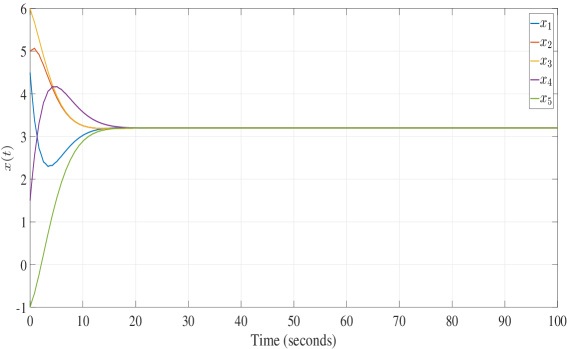
Figure 1: The states of (27) with the proposed control scheme.

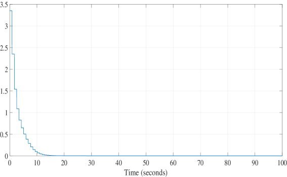
Figure 2: The value of $\underline{u}^{\mathrm{T}}\underline{u}$ of the proposed controller.

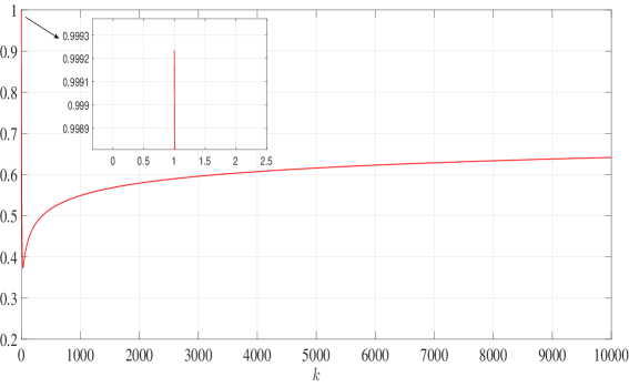
Figure 3: The value of $\big{[}\beta^{k+1}+\sum_{l=1}^{k+1}\lvert f(l)\rvert\big{]}$ under the proposed control scheme.

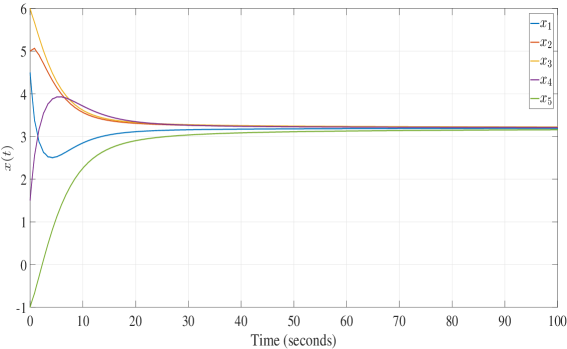
Figure 4: The states of (27) with control scheme in [21].

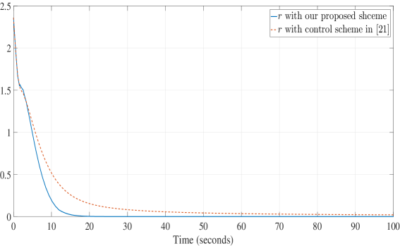
Figure 5: The mean absolute error $r$ with proposed scheme and scheme in [21].

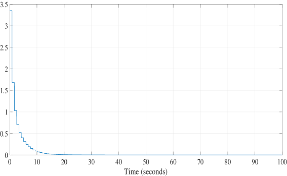
Figure 6: The value of $\underline{u}^{\mathrm{T}}\underline{u}$ of the controller in [21].

5 Conclusion

In this paper, a distributed consensus sampled-data based control scheme for multi-agent systems with fractional-order $\alpha\in(0,1)$ is proposed. By taking the hereditary and infinite memory properties of fractional-order calculus into account, a new control scheme is designed to not only ensure system stability, but also achieve asymptotic consensus. Simulation results also illustrate the accuracy and effectiveness of the proposed control algorithm.

References

- [1] J Alexander Fax and Richard M Murray. Information flow and cooperative control of vehicle formations. IEEE Transactions on Automatic Control, 49(9):1465–1476, 2004.
- [2] Jorge Cortés and Francesco Bullo. Coordination and geometric optimization via distributed dynamical systems. SIAM Journal on Control and Optimization, 44(5):1543–1574, 2005.
- [3] Wenwu Yu, Guanrong Chen, Zidong Wang, and Wen Yang. Distributed consensus filtering in sensor networks. IEEE Transactions on Systems, Man, and Cybernetics, Part B (Cybernetics), 39(6):1568–1577, 2009.
- [4] Reza Olfati-Saber and Richard M Murray. Consensus problems in networks of agents with switching topology and time-delays. IEEE Transactions on Automatic Control, 49(9):1520–1533, 2004.
- [5] Wei Wang, Jiangshuai Huang, Changyun Wen, and Huijin Fan. Distributed adaptive control for consensus tracking with application to formation control of nonholonomic mobile robots. Automatica, 50(4):1254–1263, 2014.
- [6] Wei Wang, Changyun Wen, and Jiangshuai Huang. Distributed adaptive asymptotically consensus tracking control of nonlinear multi-agent systems with unknown parameters and uncertain disturbances. Automatica, 77:133–142, 2017.
- [7] Long Cheng, Zeng-Guang Hou, Min Tan, and Xu Wang. Necessary and sufficient conditions for consensus of double-integrator multi-agent systems with measurement noises. IEEE Transactions on Automatic Control, 56(8):1958–1963, 2011.
- [8] Long Cheng, Yunpen Wang, Wei Ren, Zeng-Guang Hou, and Min Tan. On convergence rate of leader-following consensus of linear multi-agent systems with communication noises. IEEE Transactions on Automatic Control, 61(11):3586–3592, 2016.
- [9] Jiangshuai Huang, Changyun Wen, Wei Wang, and Yong-Duan Song. Adaptive finite-time consensus control of a group of uncertain nonlinear mechanical systems. Automatica, 51:292–301, 2015.
- [10] Jiangshuai Huang, Yong-Duan Song, Wei Wang, Changyun Wen, and Guoqi Li. Smooth control design for adaptive leader-following consensus control of a class of high-order nonlinear systems with time-varying reference. Automatica, 83:361–367, 2017.
- [11] Fei Chen, Zengqiang Chen, Linying Xiang, Zhongxin Liu, and Zhuzhi Yuan. Reaching a consensus via pinning control. Automatica, 45(5):1215–1220, 2009.
- [12] Min Zheng, Cheng-Lin Liu, and Fei Liu. Average-consensus tracking of sensor network via distributed coordination control of heterogeneous multi-agent systems. IEEE Control Systems Letters, 3(1):132–137, 2018.
- [13] Yongcan Cao, Yan Li, Wei Ren, and YangQuan Chen. Distributed coordination of networked fractional-order systems. IEEE Transactions on Systems, Man, and Cybernetics, Part B (Cybernetics), 40(2):362–370, 2009.
- [14] Wei Sun, Yan Li, Changpin Li, and YangQuan Chen. Convergence speed of a fractional order consensus algorithm over undirected scale-free networks. Asian Journal of Control, 13(6):936–946, 2011.
- [15] Jun Shen and Jinde Cao. Necessary and sufficient conditions for consensus of delayed fractional-order systems. Asian Journal of Control, 14(6):1690–1697, 2012.
- [16] Wenwu Yu, Yang Li, Guanghui Wen, Xinghuo Yu, and Jinde Cao. Observer design for tracking consensus in second-order multi-agent systems: Fractional order less than two. IEEE Transactions on Automatic Control, 62(2):894–900, 2016.
- [17] Milad Shahvali, Mohammad-Bagher Naghibi-Sistani, and Hamidreza Modares. Distributed consensus control for a network of incommensurate fractional-order systems. IEEE Control Systems Letters, 3(2):481–486, 2019.
- [18] Li-Sheng Hu, Tao Bai, Peng Shi, and Ziming Wu. Sampled-data control of networked linear control systems. Automatica, 43(5):903–911, 2007.
- [19] Bo Shen, Zidong Wang, and Tingwen Huang. Stabilization for sampled-data systems under noisy sampling interval. Automatica, 63:162–166, 2016.
- [20] Xiaohua Ge, Qing-Long Han, Derui Ding, Xian-Ming Zhang, and Boda Ning. A survey on recent advances in distributed sampled-data cooperative control of multi-agent systems. Neurocomputing, 275:1684–1701, 2018.
- [21] Zhiyong Yu, Haijun Jiang, Cheng Hu, and Juan Yu. Necessary and sufficient conditions for consensus of fractional-order multiagent systems via sampled-data control. IEEE Transactions on Cybernetics, 47(8):1892–1901, 2017.
- [22] Housheng Su, Yanyan Ye, Xia Chen, and Haibo He. Necessary and sufficient conditions for consensus in fractional-order multiagent systems via sampled data over directed graph. IEEE Transactions on Systems, Man, and Cybernetics: Systems, 2019.
- [23] Huiyang Liu, Guangming Xie, and Yanping Gao. Consensus of fractional-order double-integrator multi-agent systems. Neurocomputing, 340:110–124, 2019.
- [24] Jiejie Chen, Boshan Chen, and Zhigang Zeng. Synchronization and consensus in networks of linear fractional-order multi-agent systems via sampled-data control. 2019.
- [25] Yiwen Chen, Guoguang Wen, Zhaoxia Peng, and Ahmed Rahmani. Consensus of fractional-order multiagent system via sampled-data event-triggered control. Journal of the Franklin Institute, 356(17):10241–10259, 2019.
- [26] Igor Podlubny. Fractional differential equations: an introduction to fractional derivatives, fractional differential equations, to methods of their solution and some of their applications, volume 198. Elsevier, 1998.
- [27] Dingyü Xue. Fractional-order control systems: fundamentals and numerical implementations, volume 1. Walter de Gruyter GmbH & Co KG, 2017.
- [28] Vangipuram Lakshmikantham, Srinivasa Leela, and J Vasundhara Devi. Theory of fractional dynamic systems. CSP, 2009.
- [29] Changpin Li and Weihua Deng. Remarks on fractional derivatives. Applied Mathematics and Computation, 187(2):777–784, 2007.
- [30] Bijnan Bandyopadhyay and Shyam Kamal. Stabilization and control of fractional order systems: a sliding mode approach, volume 317. Springer, 2015.
- [31] Yan Li, YangQuan Chen, and Igor Podlubny. Mittag–Leffler stability of fractional order nonlinear dynamic systems. Automatica, 45(8):1965–1969, 2009.
- [32] Yan Li, YangQuan Chen, and Igor Podlubny. Stability of fractional-order nonlinear dynamic systems: Lyapunov direct method and generalized Mittag–Leffler stability. Computers & Mathematics with Applications, 59(5):1810–1821, 2010.
- [33] Fengrong Zhang, Changpin Li, and YangQuan Chen. Asymptotical stability of nonlinear fractional differential system with Caputo derivative. International Journal of Differential Equations, 2011, 2011.
- [34] Reza Olfati-Saber, J Alex Fax, and Richard M Murray. Consensus and cooperation in networked multi-agent systems. Proceedings of the IEEE, 95(1):215–233, 2007.