Adiabatic Heuristic Principle on a Torus and Generalized Streda Formula

Abstract

Although the adiabatic heuristic argument of the fractional quantum Hall states has been successful, continuous modification of the flux/statistics of anyons is strictly prohibited due to algebraic constrains of the braid group on a torus. We have numerically shown that the adiabatic heuristic principle for anyons is still valid even though the Hamiltonians cannot be modified continuously. The Chern number of the ground state multiplet is the adiabatic invariant, while the number of the topological degeneracy behaves wildly. A generalized Streda formula is proposed that explains the degeneracy pattern. Nambu-Goldston modes associated with the anyon superconductivity are also suggested numerically.

I Introduction

Over the past decade, topology has been coming to the fore in modern condensed matter physics. The quantum Hall (QH) effect Klitzing et al. (1980); Tsui et al. (1982) is a prime example of topologically non-trivial phases, where the quantized Hall conductance is given by the Chern number Thouless et al. (1982); Kohmoto (1985); Niu et al. (1985); Berry (1984). Topological concepts enrich material phases beyond the Ginzburg-Landau theory. The fractional QH (FQH) state Laughlin (1983) is a typical example of the quantum liquid with the topological order Wen (1989). It hosts fractionalized excitations that carry fractional charges and fractional statistics Arovas et al. (1984); Haldane (1983); Halperin (1984), which is the hallmark of the topologically ordered phases Wen (1995). The topological degeneracy is closely related to these fractionalizations Einarsson (1990); Wen (1989); Oshikawa and Senthil (2006); Sato et al. (2006). Some of the non-Abelian topological order can be used for a possible quantum computation Willett et al. (1987); Moore and Read (1991); Read and Rezayi (1999); Kitaev (2003); Nayak et al. (2008).

Point particles in two-dimension can be charge-flux composites associated with a singular gauge transformation Wilczek (1982). In relation to the composite fermion picture Jain (1989, 2007), the flux-attachment has been quite successful to describe the FQH effect; the FQH effect at the filling factor $\nu=p/(2mp\pm 1)$ with $p$ and $m$ integers can be understood as the $\nu=p$ IQH effect of the composite fermions. This concept is further developed to the “adiabatic heuristic principle” GREITER and WILCZEK (1990); Greiter and Wilczek (1992). It states that both states are adiabatically connected through intermediate systems of anyons. This characterization of the QH states based on the adiabatic deformation is a typical example of the topological classification as is widely applied to the recent studies of topological phases.

We note that a careful setup is required to carry the program of this adiabatic heuristic principle for concrete systems. The statistical phase $\theta$ of anyons is governed by a representation of the fundamental group of the many-particle configuration space (braid group) Wu (1984). Therefore, the world lines of the system needs to satisfy the braid group constraint.

As for topological phenomena, the geometry of the system is crucially important. With boundaries, low energy modes appear as edge states even for gapped systems. Thus, for the demonstration of the adiabatic heuristic principle, the torus geometry without any boundaries is favorable tor . However, an algebraic constraint of the braid group on a torus Birman (1969); Einarsson (1990); Wen et al. (1990); Hatsugai et al. (1991); EINARSSON (1991); LI (1993) prohibits continuous change of the statistical phase $\theta$. This makes it impossible to apply the adiabatic heuristic principle naively.

In this Letter, we show that the adiabatic heuristic principle indeed remains valid on a torus. Here, “adiabatic” is used in the sense that the gap remains open although continuous deformation of the Hamiltonian is impossible. The many-body Chern number of the ground state multiplet is also calculated numerically, which serves as the adiabatic invariant while their degeneracy changes wildly. We propose a generalized Streda formula to characterize the obtained degeneracy pattern in relation to the Chern number, which follows from the translational invariance of anyons. At the gap closing point, the Chern number changes its sign and the anyon superconductivity Laughlin (1988); Fetter et al. (1989); CHEN et al. (1989) is expected.

II Adiabatic heuristic principle and braid group

Let us here shortly derive the fundamental relation of the adiabatic heuristic principle GREITER and WILCZEK (1990); Greiter and Wilczek (1992). We consider a QH system of $N_{a}$ particles with the charge $-e$ in a uniform magnetic field. According to the adiabatic heuristic principle, the QH state is adiabatically deformed by trading the external fluxes for the statistical ones of anyons. Since the total flux remains constant ($N_{\phi}+N_{a}\theta/\pi=\text{const.}$), one has the relation $1/\nu+\theta/\pi=\text{const.}$, where $N_{\phi}$ is the number of the external flux, $\theta$ is the statistics of anyons and $\nu=N_{a}/N_{\phi}$. Assuming that the $\nu=p$ IQH state of fermions ($\theta=\pi$) is included in this series, one has $\nu=p/[p(1-\theta/\pi)+1]$.

From the analysis of the braid group on a torus Birman (1969); Einarsson (1990); Wen et al. (1990); Hatsugai et al. (1991); EINARSSON (1991); LI (1993), the relation $1/\nu+\theta/\pi=\text{const.}$ is rederived (see Appendix A) with an additional constraint as explained below. The generators of the braid group on a torus are denoted as $\sigma_{i}$, $\tau_{i}$ and $\rho_{i}$, where $\sigma_{i}$ ($i=1,\cdots,N_{a}-1$) is a local exchange between the $i$th and $i+1$th anyons, and $\tau_{i}$ and $\rho_{i}$ ($i=1,\cdots,N_{a}$) are global moves of the $i$th anyon along a noncontractible loop on the torus in $x$ and $y$ directions. Now, we take the basis $|{\{\bm{r}_{k}\};w}\rangle$ for their expressions, where $\{\bm{r}_{k}\}$ is the positions of anyons and $w=1,\cdots,M$ is the extra internal index that is necessary to satisfy the braid group constraints on a torus as seen below. We assume that anyons are Abelian: $\sigma_{i}=e^{i\theta}\bm{1}_{M}$, where $\bm{1}_{M}$ is the $M$-dimensional unit matrix. As shown in Fig. 1 Birman (1969), the generators $\sigma_{i}$, $\tau_{i}$ and $\rho_{i}$ need to satisfy

$$\tau_{i+1}^{-1}\rho_{i}\tau_{i+1}\rho_{i}^{-1}=(\sigma_{i}^{-1})^{2}=e^{-i2\theta}\bm{1}_{M}.$$ (1)

By taking a determinant of Eq. (1), we have $1=e^{-i2M\theta}$. If $\theta/\pi=n/m$ (with $n$, $m$ coprime), the dimension of the representation $M$ needs to be a multiple of $m$. This constraint strictly prohibits continuous change of the Hamiltonian in the adiabatic heuristic principle.

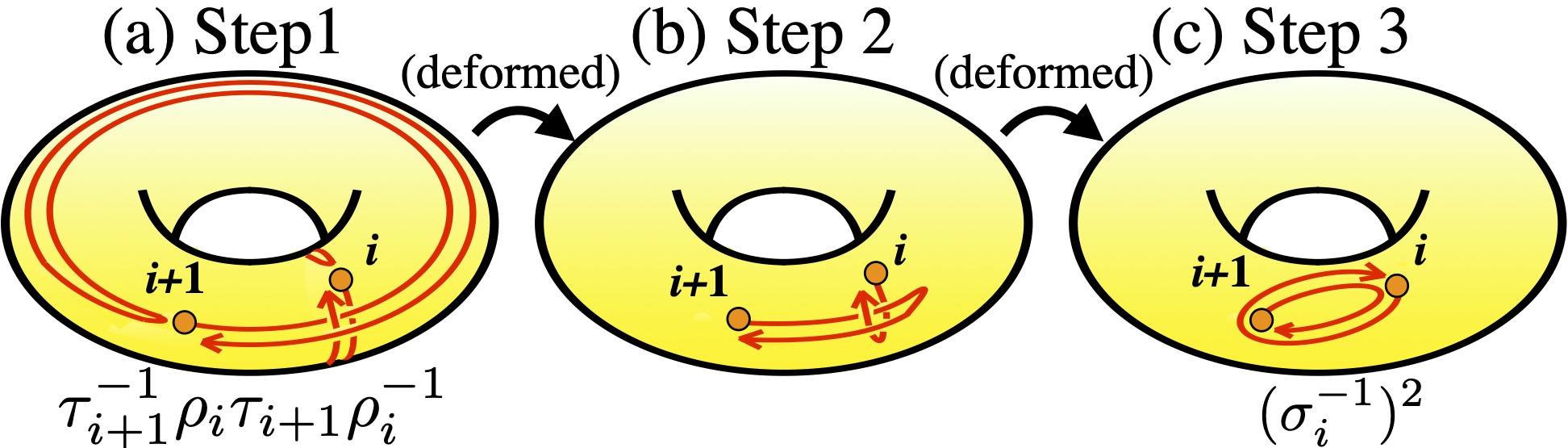
Figure 1: Pictorial proof of Eq. (1) Birman (1969). (a) The paths of the four moving processes $\rho_{i}^{-1}$, $\tau_{i+1}$, $\rho_{i}$, and $\tau_{i+1}^{-1}$ are presented in the order from bottom to top. (c) The path in (a) can be deformed into that of $(\sigma_{i}^{-1})^{2}$.

In this Letter, this puzzle is resolved. Although the Hamiltonian is defined only for discrete values of $\theta$ and its dimension behaves wildly, the energy gap defined by a dense set of the Hamiltonians is surprisingly smooth and finite. It justifies the adiabatic heuristic principle on a torus. We also find the generalized streda formula to explain the wild behavior of the degeneracy by the many-body Chern number.

III Model

We consider the periodic system of anyons in the uniform magnetic field on a square lattice with $N_{x}\times N_{y}$ sites. The Hamiltonian is

$$H=t\sum_{\langle ij\rangle}e^{i\phi_{ij}}e^{i\theta_{ij}}c_{i}^{\dagger}c_{j}\otimes W^{(ij)}+V\sum_{\langle ij\rangle}n_{i}n_{j}\otimes\bm{1}_{M},$$ (2)

where $n_{i}=c_{i}^{\dagger}c_{i}$ and $c_{i}^{\dagger}$ ($c_{i}$) is the creation (annihilation) operator for a hard-core boson on site $i$. The hard-core condition is necessary to ensure consistency with the braid group. The Peierls phase $e^{i\phi_{ij}}$ is specified by the string gauge Hatsugai et al. (1999) for the external magnetic field. The phase $e^{i\theta_{ij}}$ describes the statistical phase Wen et al. (1990); Hatsugai et al. (1991) (see the details below). $W^{(ij)}$ is an $M$-dimensional matrix Hatsugai et al. (1991) to ensure consistency with Eq. (1). When $\theta/\pi=n/m$, $M$ is fixed to be $m$ as the irreducible representation. We set $W^{(ij)}=W_{x}$ and $W_{y}$ for $(ij)$ describing a pair of sites across the boundary in the $x$ and $y$ directions respectively and otherwise $W^{(ij)}=\bm{1}_{M}$, where

$$W_{x} =\left[\begin{array}[]{cccc}0&1&\ldots&0\\ \vdots&\vdots&\ddots&\vdots\\ 0&0&\ldots&1\\ e^{i\eta_{x}}&0&\ldots&0\end{array}\right],$$ (7)

$$W_{y} =e^{i\eta_{y}}\text{diag}[e^{i2\theta},e^{i4\theta},\cdots,e^{i2M\theta}],$$ (8)

and $\vec{\eta}=(\eta_{x},\eta_{y})$ specifies the twisted boundary conditions. The Hamiltonian is consistent with Eq. (1) since we have $W_{x}^{-1}W_{y}W_{x}W_{y}^{-1}=e^{-i2\theta}\bm{1}_{M}$ for any $\vec{\eta}$.

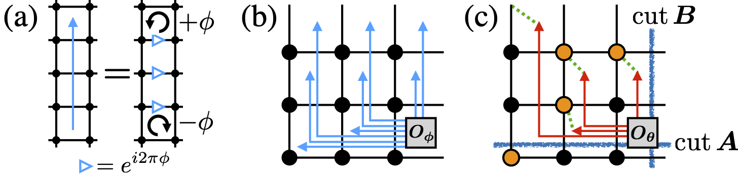
Figure 2: (a) String gauge. (b)(c) Sketches of $3\times 3$ square lattice with (b) the string gauge $\phi_{ij}$ and (c) the statistical gauge $\theta_{ij}$. The yellow points in (c) represent sites with anyons.

Let us now give detailed descriptions of how to construct the Hamiltonian in Eq. (2). We first mention the string gauge $\phi_{ij}$ briefly. As shown in Fig. 2(a), let us consider a string on sites and assigns the Peierls phase $e^{i2\pi\phi}$ on the links intersected by the string. They clearly describe the magnetic fluxes $\phi$ and $-\phi$ at the initial and terminal points of the string, respectively. Thus, the string gauge shown in Fig. 2(b) introduces the flux $\phi\times(1-N_{x}N_{y})$ to the plaquette with the origin $O_{\phi}$ while $\phi$ to the others. The gauge convention $\theta_{ij}$ is also described by the strings, see Fig. 2(c). The strings carry the phase factor $e^{i\theta}$, and their terminal points are located at plaquettes adjoining anyons. Besides, the additional rules are given as follows Hatsugai et al. (1991): (The roles of each rule are explained in Ref. rul, )

(i) If a string sweeps another anyon in the process of hopping, one determines the phase factor as if the anyon crosses the string.

(ii) When an anyon hops across the cut $B$ from left to right, the phase factor $e^{i(N_{a}-1)\theta}$ is given.

(iii) When an anyon hops across a horizontal string, the phase factor not $e^{i\theta}$ but $e^{i2\theta}$ is given.

(iv) When an anyon hops across the cut $A$ upward, the phase factor $e^{iX\theta}$ is given, where $X$ is the number of other anyons in the same $x$-axis position as the hopping anyon.

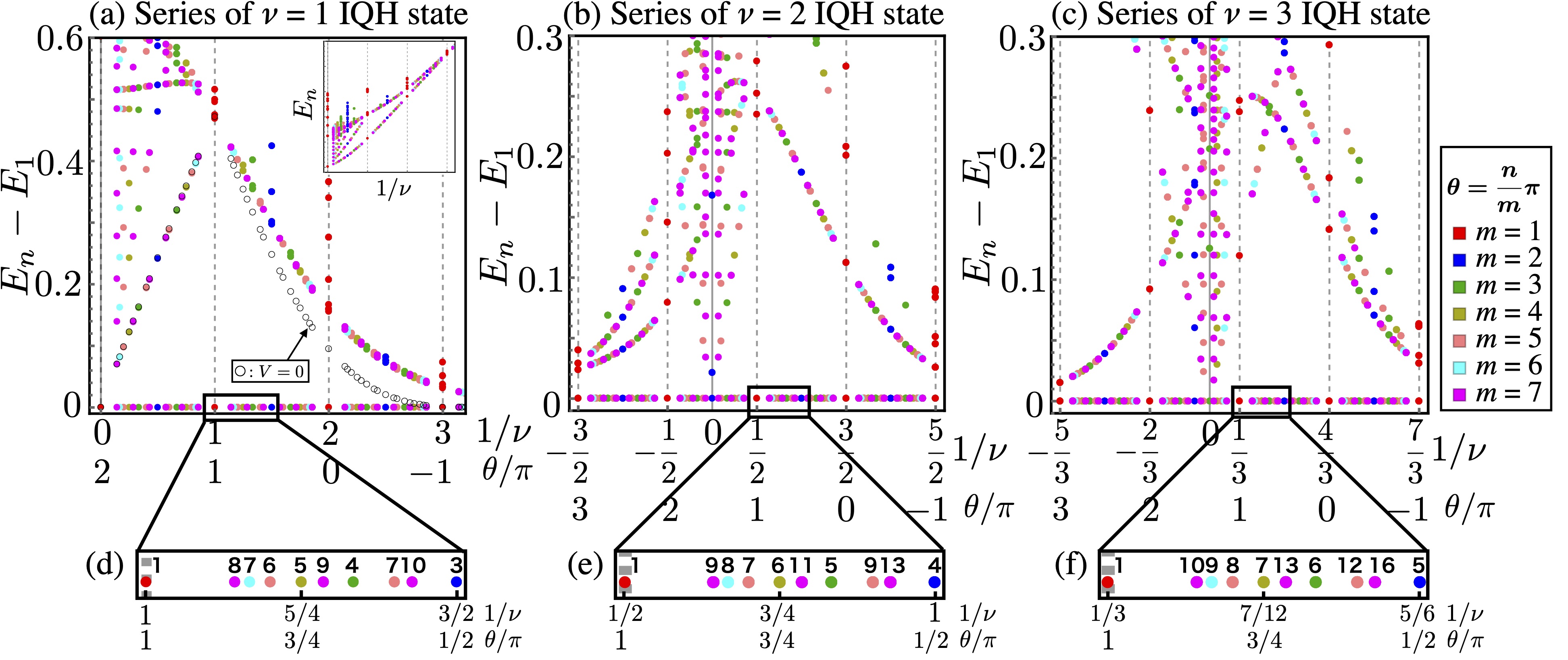
Figure 3: (a-c) Energy gaps are shown as functions of $1/\nu$ for $t=-1$ and $V=5$. The system size is $N_{x}\times N_{y}=10\times 10$. The statistical parameter $\theta$ is determined by $\nu=p/[p(1-\theta/\pi)+1]$ with (a) $p=1$ (b) $p=2$, and (c) $p=3$, respectively. The vertical dashed lines represent $\theta/\pi=\text{integer}$. The anyon number is (a),(b) $N_{a}=4$ and (c) $N_{a}=3$. We plot the lowest $N_{\text{cut}}$ states at each $1/\nu$ in the figures [$N_{\text{cut}}=40$ for (a) and (b), and $N_{\text{cut}}=70$ for (c)]. The open black circles in (a) are the gaps $E_{N_{D}+1}-E_{1}$ for $V=0$. The inset in (a) is the energy spectrum of the same setting as (a). (d-f) Ground state degeneracy $N_{D}$ is shown.

Due to Eqs. (7) and (8), we also give the following rules: When an anyon hops across the cut $B$ from left to right, the label is changed from $w$ to $w-1$, where $w$ is the label of the basis $|{\{\bm{r}_{k}\};w}\rangle$. If $w=1$, the phase factor $e^{i\eta_{x}}$ is also given. Also, when an anyon hops across the cut $A$ upward, the phase factor $e^{i\eta_{y}}e^{i2w\theta}$ is given.

In this framework, the representations of the global move operators are given as $\tau_{j}=e^{i\frac{e}{\hbar}\alpha_{j}}e^{-i2\theta(j-1)}W_{x}$ and $\rho_{j}=e^{i\frac{e}{\hbar}\beta_{j}}e^{i2\theta(j-1)}W_{y}$, where $e^{i\frac{e}{\hbar}\alpha_{j}}$ and $e^{i\frac{e}{\hbar}\beta_{j}}$ are came from the Peierls phase $\phi_{ij}$ describing the external magnetic field. As shown in Appendix A, these representations are consistent with the braid group on a torus.

The above construction of $\theta_{ij}$ introduces the magnetic flux $-2\pi\times 2\theta N_{a}$ only to the plaquette with the origin $O_{\theta}$ shown in Fig. 2(c) Hatsugai et al. (1991). Since the string gauge $\phi_{ij}$ introduces the flux $\phi\times(1-N_{x}N_{y})$ to the plaquette with the origin $O_{\phi}$ while $\phi$ to the others as described above, one gets a condition of the uniformity of the magnetic field as $e^{i2\pi\phi(1-N_{x}N_{y})-i2\theta N_{a}}=e^{i2\pi\phi}$. Since $N_{\phi}=\phi N_{x}N_{y}$, this condition is consistent with the relation $1/\nu+\theta/\pi=\text{const.}$

IV Energy gap

By the above setup, we numerically diagonalize the Hamiltonians. In the following, we set $N_{x}=N_{y}=10$, $t=-1$, $V=5$ and $\vec{\eta}=\vec{0}$ unless otherwise stated. We assume that the states are degenerate if the energy difference is less than $0.001$.

In Figs. 3(a)-(c), we plot the energies of a series that includes the $\nu=p$ IQH state ($p=1,2,3$) as a function of $1/\nu$. We show the data for $\theta=(n/m)\pi$ with various $m$ and $n$ ($m\leq 7$). The data points with different colors are eigenvalues of $H$ with the different dimensions. Figures 3(a)-(c) show that the gap behaves smoothly for a dense set of Hamiltonians. The energies of the ground state are also smooth, see the inset in Fig. 3(a).

Let us first consider a series of the $\nu=1$ IQH state, which includes the Laughlin state. We here consider only $0\leq\nu$ since a system of $\nu<0$ is trivially mapped to that of $0<\nu$. In Fig. 3(a), the 3-fold degenerated ground state is obtained at $\nu=1/3$ , which is consistent with the lattice analogue of the Laughlin state Kudo et al. (2017). This state is adiabatically connected to the $\nu=1$ IQH state. Note that, however, the ground state degeneracy $N_{D}$ changes wildly, see Fig. 3(d). At $1/\nu=0$, the gap closing occurs, which suggests the Nambu-Goldston modes associated with the superconductivity of hard-core bosons ZHANG (1992). In Fig 3(a), the results without the electron-electron interactions are also shown. While the ground states of anyons or bosons are gapped because of their hard-core nature, the gap at $\nu=1/3$ vanishes since the system reduces to the partially filled lowest Landau band of free fermions. It implies that the interaction is crucially important only for the FQH states of fermions. In Fig. 4, the energy spectra as functions of the interaction $V$ are shown. The FQH states remain gapped with the same topological degeneracy for a wide range of $V$ apart from the point $V=0$ in Fig. 4(c). Inclusion of the finite interaction $V$ induces the gap at this point, which is consistent with the gapped Laughlin state. Although the discussion of the thermodynamic limit is an open question, our adiabatic heuristic argument for the fixed system size includes important scientific information.

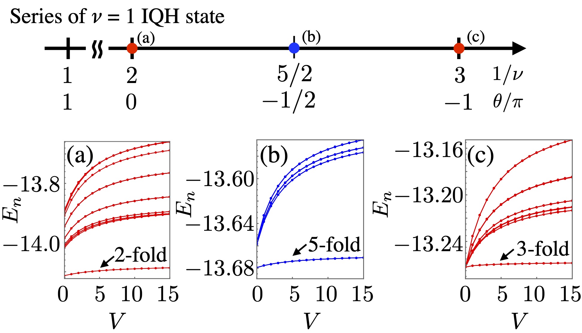
Figure 4: Energy spectra are shown as functions of the interaction $V$ for (a) the Boson FQH state at $\nu=1/2$, (b) the anyon FQH state at $\nu=2/5$ and (c) the Fermion FQH state at $\nu=1/3$. They are included in a series of the $\nu=1$ IQH state. We set $t=-1$ and $N_{x}\times N_{y}=10\times 10$. The lowest forty states are shown in each figure.

As for the other series in Figs. 3(b) and (c), one can also see that the gaps remain open for each region $0<1/\nu$ and $1/\nu<0$ although their topological degeneracy changes irregularly [see Figs. 3(e) and (f)]. The excitation gap closes at $1/\nu=0$ in both figures, which is consistent with the emergence of the anyon superconductivity Laughlin (1988); Fetter et al. (1989); CHEN et al. (1989) of $\theta=(3/2)\pi$ and $\theta=(4/3)\pi$, respectively.

The numerical results in Figs. 3 suggest that the adiabatic heuristic principle remains valid for a series that includes $\nu=p$ IQH state for general integer $p$. It also suggests the realization of the anyon superconductivity of $\theta=(1+1/p)\pi$ by trading all the external magnetic flux for the statistical one.

Since $1/\nu\propto\phi$, where $\phi=N_{\phi}/(N_{x}N_{y})$ is the number of the flux per plaquette, this unusual but adiabatic behavior, in a sense that the gap remains open, is similar to the Azbel-Hofstadter problem Azb ; Hofstadter (1976); Hasegawa et al. (1990) for the weak magnetic field limit. It implies that the adiabatic invariant of the evolution can be given by the Chern number of the ground state multiplet. This is correct as we discuss below.

V Adiabatic invariant

As for the gapped ground state multiplet of anyons, we calculate the many-body Chern number Niu et al. (1985)

$$C=\frac{1}{2\pi i}\int_{T^{2}}d^{2}\eta F,$$ (9)

where $T^{2}=[0,2\pi]\times[0,2\pi]$, $F=(\partial A_{y}/\partial\eta_{x})-(\partial A_{x}/\partial\eta_{y})$, $A_{x(y)}=\text{Tr\,}[\Phi^{\dagger}(\partial\Phi/\partial\eta_{x(y)})]$ and $\Phi=\left(|{G_{1}}\rangle\cdots,|{G_{N_{D}}}\rangle\right)$ is a ground state multiplet. In the numerical calculation, we use the method proposed in Ref. Fukui et al., 2005.

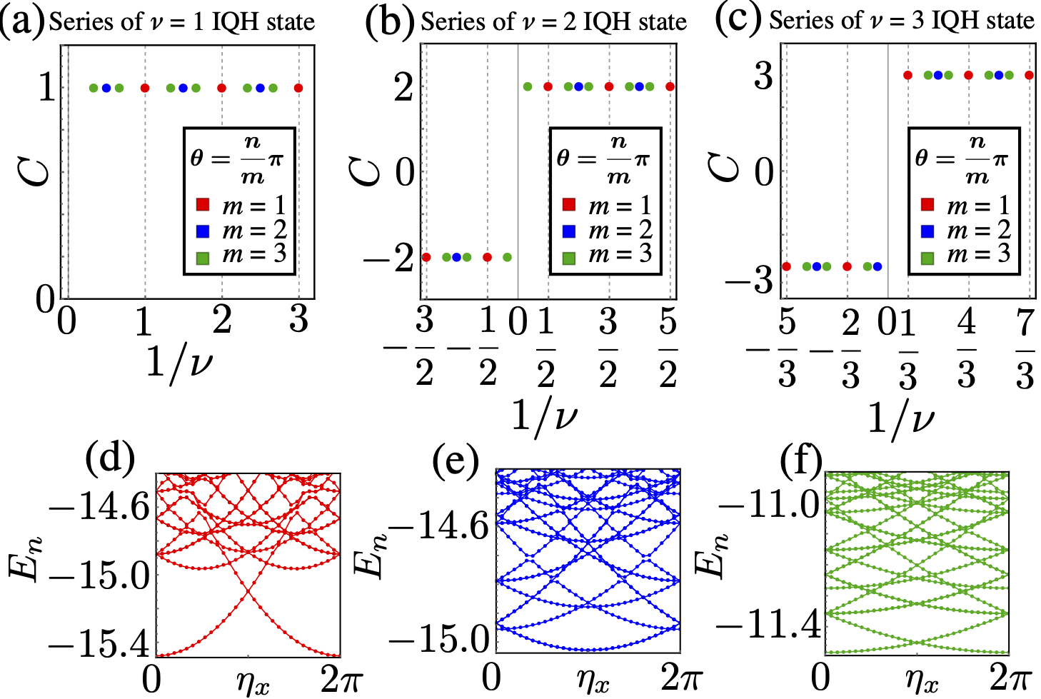
Figure 5: (a)-(c) Chern number $C$ of the degenerated ground state multiplet are shown as functions of $1/\nu$. In (a), (b) and (c), we consider the systems in the same setting as Fig. 3(a), (b) and (c), respectively. (d)-(f) Spectral flows at $1/\nu=0$ for each series. We set $\eta_{y}=0$. The statistics parameter is given by (d) $\theta/\pi=2$, (e) $\theta/\pi=3/2$ and (f) $\theta/\pi=4/3$, respectively.

In Figs 5(a-c), we plot $C$ for the systems of the same setting as Figs. 3(a-c). Although the dimensions of the multiplet changes wildly, the Chern number $C$ remains the same. It suggests that $C$ is an adiabatic invariant of the evolution. As for a series that includes the $\nu=p$ IQH state, we numerically obtain

$$C=\text{sgn}(\nu)\times p,$$ (10)

where $\text{sgn}(x)$ is the sign function. For $\nu>0$, Eq. (10) is natural since the $\nu=p$ IQH state is included. However, the case of $\nu<0$ is non-trivial since it does not include any simple state.

While the energy of the QH systems is almost independent of $\vec{\eta}$, the spectral flows at $1/\nu=0$ exhibit the strong $\vec{\eta}$ dependences, see Figs. 5(d-f). They indicate the absence of the energy gap at $1/\nu=0$, which implies the Nambu-Goldston modes of the anyon superconductors.

VI Topological degeneracy

As mentioned above, the ground state degeneracy changes wildly during the evolution as shown in Figs. 3(d-f). The fermion FQH state at $\nu=p/q$ is $q$-fold degenerated Haldane (1985) but this pattern does not hold in the anyonic systems; the QH state with $(\nu,\theta/\pi)=(1,1/2)$ in Fig. 3(e), for example, has $4$-fold degeneracy. We address this issue analytically below.

Let us consider a continuous translational invariant system of the size $L_{x}\times L_{y}$ with external magnetic field $B=\phi_{0}N_{\phi}/(L_{x}L_{y})$. The results obtained below is valid even for lattice models as long as $\phi$ is sufficiently small, i.e., the magnetic length becomes much larger than the lattice constant. The statistics of anyons is set $\theta=(n/m)\pi$ and a translation operator of center-of-mass is given by $T(\bm{a})=\exp\{{(i/\hbar)\sum_{i}\bm{K}_{i}\cdot\bm{a}}\}$, where $\bm{K}_{i}=\bm{p}_{i}+e\bm{A}(\bm{r}_{i})-eB\bm{e}_{z}\times\bm{r}_{i}$ Zak (1964); Haldane (1985); Tao and Haldane (1986). Since the interactions of the system including the statistical vector potential Wilczek (1982) are given by the relative coordinates of anyons, $T(\bm{a})$ commutes with the Hamiltonian $H$. Noting that $T(\bm{b})^{-1}T(\bm{a})^{-1}T(\bm{b})T(\bm{a})=e^{i\frac{e}{\hbar}B(\bm{a}\times\bm{b})N_{a}}$, let us now assume the followings

$$\rho_{i}^{-1}T(\bm{a})^{-1}\rho_{i}T(\bm{a})=e^{i\frac{e}{\hbar}B(\bm{a}\times L_{y}\bm{e}_{y})}$$ (11)

$$T(\bm{b})^{-1}\tau_{i}^{-1}T(\bm{b})\tau_{i}=e^{i\frac{e}{\hbar}B(L_{x}\bm{e}_{x}\times\bm{b})},$$ (12)

since each loop given by Eqs. (11) and  (12) does not enclose the other anyons.

Equation (1) implies $[\tau_{i}^{m},\rho_{j}]=0$. (The proof for any $i$ and $j$ is given in Appendix A). Then by defining $\mathcal{T}_{A}\equiv T(\frac{1}{m}\frac{L_{y}}{N_{\phi}}\bm{e}_{y})$, which satisfies

$$[\mathcal{T}_{A},\tau_{i}^{m}]=[\mathcal{T}_{A},\rho_{i}]=0,$$ (13)

let us take the simultaneous eigenstate $|{\psi_{0}}\rangle$, which satisfies $H(\vec{\eta})|{\psi_{0}}\rangle=E(\vec{\eta})|{\psi_{0}}\rangle$ and $\mathcal{T}_{A}|{\psi_{0}}\rangle=e^{i\lambda}|{\psi_{0}}\rangle$ with $\lambda$ real. Here, the twisted boundary angles $\vec{\eta}$ are specified by $\tau_{i}^{m}$ and $\rho_{i}$ with Eqs. (7) and  (8). Further defining $\mathcal{T}_{B}\equiv T(\frac{L_{x}}{N_{\phi}}\bm{e}_{x})$ and $\mathcal{T}_{C}\equiv\tau_{1}T(\frac{n}{m}\frac{L_{x}}{N_{\phi}}\bm{e}_{x})$, we define a new state $|{\psi_{s,t}}\rangle\equiv\mathcal{T}_{B}^{s}\mathcal{T}_{C}^{t}\,|{\psi_{0}}\rangle$. While $\mathcal{T}_{B}$ and $\mathcal{T}_{C}$ commute with $\tau^{m}_{i}$ and $\rho_{i}$, we have

$$\mathcal{T}_{A}\mathcal{T}_{B}=\mathcal{T}_{B}\mathcal{T}_{A}e^{i2\pi\frac{1}{m}\nu},$$ (14)

$$\mathcal{T}_{A}\mathcal{T}_{C}=\mathcal{T}_{C}\mathcal{T}_{A}e^{i2\pi(\frac{1}{m}+\nu\frac{n}{m^{2}})}.$$ (15)

It implies $H(\vec{\eta})|{\psi_{s,t}}\rangle=E(\vec{\eta})|{\psi_{s,t}}\rangle$ and $\mathcal{T}_{A}|{\psi_{s,t}}\rangle=e^{i\lambda}e^{i2\pi f_{s,t}}|{\psi_{s,t}}\rangle$ with

$$f_{s,t}=\frac{\nu s+\left(1+\nu\theta/\pi\right)t}{m}=\frac{\nu}{pm}\left(p\left(s+t\right)+t\right),$$ (16)

where $\nu=p/[p(1-\theta/\pi)+1]$ is used at the last part. Thus, the topological degeneracy $N_{\text{TD}}$ is given by the number of pairs $(s,t)$ that give different values of $f_{s,t}\mod 1$. Since $pm/\nu$ is always integer, one obtains $N_{\text{TD}}=pm/|\nu|$. Using Eq. (10) and $M=m$ (irreducible representation), we have

$$N_{\text{TD}}=MC/\nu.$$ (17)

This is consistent with the obtained ground state degeneracy shown in Fig. 3(d-f). Anyon nature shown in Eq. (15) gives the extra degeneracy compared with the fermionic standard case Haldane (1985).

VII Generalized Streda formula

Taking difference of Eq. (17) for two possible cases in a series, one obtains $\Delta N_{\text{TD}}/\Delta(M/\nu)=C$, where we assume the Chern number $C$ is the invariant. Since $M/\nu=MN_{x}N_{y}\phi/N_{a}$ with $\phi$ the number of the flux per plaquette, we finally have

$$\frac{\Delta(N_{p}/N^{\prime}_{\text{site}})}{\Delta\phi}=C,$$ (18)

where $N_{p}\equiv N_{\text{TD}}N_{a}$ is the “parton” number corrected by the topological degeneracy and $N^{\prime}_{\text{site}}\equiv MN_{x}N_{y}$ is the extended number of sites due to the non-Abelian nature of the representation. This is a generalized Streda formula for anyons. Note that Eq. (18) for fermions ($M=1$, $\nu=p/q$, $N_{\text{TD}}=q$, $C=p$) reduces to the standard Streda formula Streda (1982). When one includes a reducible representation of the braid group, i.e., $M=tm$ with $2\leq t$ ($t$: integer), the degeneracy $N_{\text{TD}}$ increases by $t$ times. Therefore, Eqs. (17) and (18) holds generally.

VIII Conclusion

In this Letter, the adiabatic heuristic principle for the QH states is demonstrated on a torus numerically. The emergence of the anyon superconducting states is also suggested. The Chern number of the ground state multiplet serves as the adiabatic invariant of the evolution although their degeneracy changes wildly. The anyon nature brings the extra multiplicity to the topological degeneracy. It results in a generalized Streda formula that follows from the translational invariance. Extensions of this adiabatic principle on a torus can be useful to characterize the non-Abelian FQH states.

Appendix A Constraints on statistical phase

In this appendix, we derive the relation $1/\nu+\theta/\pi=\text{const.}$ from the braid group analysis on a torus. Also, a proof of $[\tau_{i}^{m},\rho_{j}]=0$ for any $i$ and $j$ is also given here.

In the main text, we denote the generators of the braid group on a torus by $\sigma_{i}$, $\tau_{i}$ and $\rho_{i}$. They satisfy the following relations Einarsson (1990); EINARSSON (1991); LI (1993):

$$\tau_{i+1}^{-1}\rho_{i}\tau_{i+1}\rho_{i}^{-1}=(\sigma_{i}^{-1})^{2},$$ (19)

$$\rho_{1}^{-1}\tau_{1}^{-1}\rho_{1}\tau_{1}=\sigma_{1}\cdots\sigma_{N_{a}-1}\sigma_{N_{a}-1}\cdots\sigma_{1}e^{i\frac{e}{\hbar}BL_{x}L_{y}},$$ (20)

$$\tau_{i+1}=\sigma_{i}^{-1}\tau_{i}\sigma_{i}^{-1}e^{i\frac{e}{\hbar}(\alpha_{i+1}-\alpha_{i})},$$ (21)

$$\rho_{i+1}=\sigma_{i}\rho_{i}\sigma_{i}e^{i\frac{e}{\hbar}(\beta_{i+1}-\beta_{i})},$$ (22)

where $\alpha_{i}$ and $\beta_{i}$ are real numbers. Equation (19) is the same as Eq. (1). The derivations of Eqs. (21) and  (22) are given in Appendix B.

Substituting $\sigma_{i}=e^{i\theta}\bm{1}_{M}$ into Eqs. (19), (20), (21) and (22), we have

$$\rho_{i}\tau_{i+1}=\tau_{i+1}\rho_{i}e^{-i2\theta},$$ (23)

$$\rho_{1}\tau_{1}=\tau_{1}\rho_{1}e^{i2(N_{a}-1)\theta+i2\pi N_{\phi}},$$ (24)

$$\tau_{i+1}=\tau_{i}e^{-i2\theta}e^{i\frac{e}{\hbar}(\alpha_{i+1}-\alpha_{i})},$$ (25)

$$\rho_{i+1}=\rho_{i}e^{i2\theta}e^{i\frac{e}{\hbar}(\beta_{i+1}-\beta_{i})}.$$ (26)

Here, we note that the representations

$$\tau_{j} =e^{i\frac{e}{\hbar}\alpha_{j}}e^{-i2\theta(j-1)}W_{x},$$ (27)

$$\rho_{j} =e^{i\frac{e}{\hbar}\beta_{j}}e^{i2\theta(j-1)}W_{y},$$ (28)

satisfy the relations in Eqs. (23), (24), (25) and (26). Substituting Eq. (25) into Eq. (23), one gets

$$\rho_{i}\tau_{j}=\tau_{j}\rho_{i}e^{-i2\theta}.$$ (29)

If $\theta/\pi=n/m$, it reduces to $[\tau_{i}^{m},\rho_{j}]=0$. Comparing Eq. (29) for $i=j=1$ with Eq. (24), we get

$$e^{i2\theta N_{a}+i2\pi N_{\phi}}=1.$$ (30)

It implies that $\theta/\pi+1/\nu=2\pi s/N_{a}$ with $s$ integer.

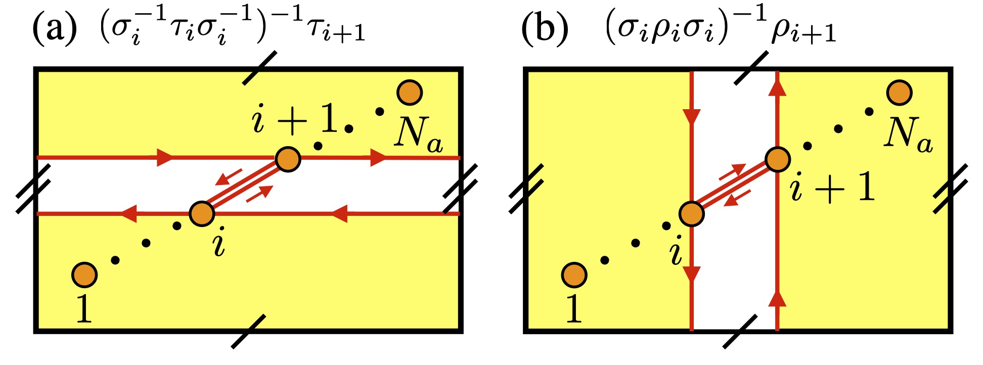
Figure 6: Closed paths defined by (a) $(\sigma_{i}^{-1}\tau_{i}\sigma_{i}^{-1})^{-1}\tau_{i+1}$ and $(\sigma_{i}\rho_{i}\sigma_{i})^{-1}\rho_{i+1}$.

Appendix B Noncontractible loops on a torus

In this appendix, we prove Eqs. (21) and (22). If the magnetic flux is absent, the relations of the braid group are given as Birman (1969); Einarsson (1990)

$$\tau_{i+1} =\sigma_{i}^{-1}\tau_{i}\sigma_{i}^{-1},$$ (31)

$$\rho_{i+1} =\sigma_{i}\rho_{i}\sigma_{i}.$$ (32)

Note that $(\sigma_{i}^{-1}\tau_{i}\sigma_{i}^{-1})^{-1}\tau_{i+1}$ and $(\sigma_{i}\rho_{i}\sigma_{i})^{-1}\rho_{i+1}$ move anyons along closed loops shown in Figs. 6(a) and (b), respectively. Therefore, if the magnetic field described by the vector potential $\bm{A}(\bm{r})$ is present, $(\alpha_{i+1}-\alpha_{i})/\phi_{0}$ and $(\beta_{i+1}-\beta_{i})/\phi_{0}$ fluxes penetrate each closed paths, respectively, where $\alpha_{i}=\oint_{L_{\tau_{i}}}d\bm{r}\cdot\bm{A}(\bm{r})$, $\beta_{i}=\oint_{L_{\rho_{i}}}d\bm{r}\cdot\bm{A}(\bm{r})$, and $L_{\tau_{i}(\rho_{i})}$ is the path given by $\tau_{i}(\rho_{i})$. Then we obtain Eqs. (21) and (22).

References

- Klitzing et al. (1980) K. v. Klitzing, G. Dorda, and M. Pepper, Phys. Rev. Lett. 45, 494 (1980).
- Tsui et al. (1982) D. C. Tsui, H. L. Stormer, and A. C. Gossard, Phys. Rev. Lett. 48, 1559 (1982).
- Thouless et al. (1982) D. J. Thouless, M. Kohmoto, M. P. Nightingale, and M. den Nijs, Phys. Rev. Lett. 49, 405 (1982).
- Kohmoto (1985) M. Kohmoto, Annals of Physics 160, 343 (1985).
- Niu et al. (1985) Q. Niu, D. J. Thouless, and Y.-S. Wu, Phys. Rev. B 31, 3372 (1985).
- Berry (1984) M. V. Berry, Proceedings of the Royal Society of London. A. Mathematical and Physical Sciences 392, 45 (1984).
- Laughlin (1983) R. B. Laughlin, Phys. Rev. Lett. 50, 1395 (1983).
- Wen (1989) X. G. Wen, Phys. Rev. B 40, 7387 (1989).
- Arovas et al. (1984) D. Arovas, J. R. Schrieffer, and F. Wilczek, Phys. Rev. Lett. 53, 722 (1984).
- Haldane (1983) F. D. M. Haldane, Phys. Rev. Lett. 51, 605 (1983).
- Halperin (1984) B. I. Halperin, Phys. Rev. Lett. 52, 1583 (1984).
- Wen (1995) X.-G. Wen, Advances in Physics 44, 405 (1995).
- Einarsson (1990) T. Einarsson, Phys. Rev. Lett. 64, 1995 (1990).
- Oshikawa and Senthil (2006) M. Oshikawa and T. Senthil, Phys. Rev. Lett. 96, 060601 (2006).
- Sato et al. (2006) M. Sato, M. Kohmoto, and Y.-S. Wu, Phys. Rev. Lett. 97, 010601 (2006).
- Willett et al. (1987) R. Willett, J. P. Eisenstein, H. L. Störmer, D. C. Tsui, A. C. Gossard, and J. H. English, Phys. Rev. Lett. 59, 1776 (1987).
- Moore and Read (1991) G. Moore and N. Read, Nuclear Physics B 360, 362 (1991).
- Read and Rezayi (1999) N. Read and E. Rezayi, Phys. Rev. B 59, 8084 (1999).
- Kitaev (2003) A. Kitaev, Annals of Physics 303, 2 (2003).
- Nayak et al. (2008) C. Nayak, S. H. Simon, A. Stern, M. Freedman, and S. Das Sarma, Rev. Mod. Phys. 80, 1083 (2008).
- Wilczek (1982) F. Wilczek, Phys. Rev. Lett. 49, 957 (1982).
- Jain (1989) J. K. Jain, Phys. Rev. Lett. 63, 199 (1989).
- Jain (2007) J. K. Jain, Composite Fermions (Cambridge University Press, 2007).
- GREITER and WILCZEK (1990) M. GREITER and F. WILCZEK, Modern Physics Letters B 04, 1063 (1990).
- Greiter and Wilczek (1992) M. Greiter and F. Wilczek, Nuclear Physics B 370, 577 (1992).
- Wu (1984) Y.-S. Wu, Phys. Rev. Lett. 52, 2103 (1984).
- (27) Since the system of anyons is intrinsically a many-body problem, the construction of the pseudopotential projected into the lowest Landau level is impossible. Therefore, we choose a toroidal lattice model for the direct numerical demonstrations. This geometry is also suitable for evaluation of the topological numbers.
- Birman (1969) J. S. Birman, Communications on Pure and Applied Mathematics 22, 41 (1969).
- Wen et al. (1990) X. G. Wen, E. Dagotto, and E. Fradkin, Phys. Rev. B 42, 6110 (1990).
- Hatsugai et al. (1991) Y. Hatsugai, M. Kohmoto, and Y.-S. Wu, Phys. Rev. B 43, 10761 (1991).
- EINARSSON (1991) T. EINARSSON, Modern Physics Letters B 05, 675 (1991).
- LI (1993) D. LI, International Journal of Modern Physics B 07, 2779 (1993).
- Laughlin (1988) R. B. Laughlin, Phys. Rev. Lett. 60, 2677 (1988).
- Fetter et al. (1989) A. L. Fetter, C. B. Hanna, and R. B. Laughlin, Phys. Rev. B 39, 9679 (1989).
- CHEN et al. (1989) Y.-H. CHEN, F. WILCZEK, E. WITTEN, and B. I. HALPERIN, International Journal of Modern Physics B 03, 1001 (1989).
- Hatsugai et al. (1999) Y. Hatsugai, K. Ishibashi, and Y. Morita, Phys. Rev. Lett. 83, 2246 (1999).
- (37) The rule (i) ensures the local exchange operation. The rules (ii) and (iii) remove the artificial twisted boundary condition in the - and -direction caused by anyon fluxes, respectively. Necessity of the rule (iv) comes from ordering vertical anyon strings of particles in the same -axis position as the hopping anyon.
- Kudo et al. (2017) K. Kudo, T. Kariyado, and Y. Hatsugai, Journal of the Physical Society of Japan 86, 103701 (2017).
- ZHANG (1992) S. C. ZHANG, International Journal of Modern Physics B 06, 25 (1992).
- (40) M. Y. Azbel, ZhETF 46, 929 (1964) [J. Exp. Theor. Phys. 19, 634 (1964)].
- Hofstadter (1976) D. R. Hofstadter, Phys. Rev. B 14, 2239 (1976).
- Hasegawa et al. (1990) Y. Hasegawa, Y. Hatsugai, M. Kohmoto, and G. Montambaux, Phys. Rev. B 41, 9174 (1990).
- Fukui et al. (2005) T. Fukui, Y. Hatsugai, and H. Suzuki, Journal of the Physical Society of Japan 74, 1674 (2005).
- Haldane (1985) F. D. M. Haldane, Phys. Rev. Lett. 55, 2095 (1985).
- Zak (1964) J. Zak, Phys. Rev. 134, A1602 (1964).
- Tao and Haldane (1986) R. Tao and F. D. M. Haldane, Phys. Rev. B 33, 3844 (1986).
- Streda (1982) P. Streda, Journal of Physics C: Solid State Physics 15, L717 (1982).