Robust Single-Image Super-Resolution via CNNs and TV-TV Minimization

Abstract

Single-image super-resolution is the process of increasing the resolution of an image, obtaining a high-resolution (HR) image from a low-resolution (LR) one. By leveraging large training datasets, convolutional neural networks (CNNs) currently achieve the state-of-the-art performance in this task. Yet, during testing/deployment, they fail to enforce consistency between the HR and LR images: if we downsample the output HR image, it never matches its LR input. Based on this observation, we propose to post-process the CNN outputs with an optimization problem that we call TV-TV minimization, which enforces consistency. As our extensive experiments show, such post-processing not only improves the quality of the images, in terms of PSNR and SSIM, but also makes the super-resolution task robust to operator mismatch, i.e., when the true downsampling operator is different from the one used to create the training dataset.

I Introduction

In science and engineering, images acquired by sensing devices often have resolution well below the desired one. Common reasons include physical constraints, as in astronomy or biological microscopy, and cost, as in consumer electronics or medical imaging. Creating high-resolution (HR) images from low-resolution (LR) ones, a task known as super-resolution (SR), can therefore be extremely useful in these areas; it enables, for example, the identification of structures or objects that are barely visible in LR images. Doing so, however, requires inferring values for the unobserved pixels, which cannot be done without making assumptions about the class of images to super-resolve and their acquisition process.

Classical interpolation algorithms assume that the missing pixels can be inferred by linearly combining neighboring pixels via, e.g., the application of filters [3, 4], or by preserving the statistics of the image gradient from the LR to the HR image [5]. Reconstruction-based methods, on the other hand, assume that images have sparse representations in some domain, e.g., sparse gradients [6, 7, 8, 9, 10, 11, 12, 13]. More recently, data-driven methods have become very popular; their main assumption is that image features can be learned from training data, via dictionaries [14, 15] or via convolutional neural networks (CNNs) [16, 17, 18].

CNNs were first applied to image SR in the seminal work [16] and have ever since remained the state-of-the-art, both in terms of reconstruction performance and computational complexity (during deployment/testing). By relying on vast databases of images for training, such as ImageNet [19] or T91 [14], they can effectively learn to map LR images/patches to HR images/patches. Although training a CNN can take several days, applying it to an image (what is typically called the testing phase) takes a few seconds or even sub-seconds. Despite these advantages, the knowledge that CNNs extract from data is never made explicit, making them hard to adapt to new scenarios: for example, simply changing the scaling factor or the sampling model, e.g., from bicubic to point sampling, almost always requires retraining the entire network. More conspicuously, however, is that during testing SR CNNs fail to guarantee the consistency between the reconstructed HR image and the input LR image, effectively ignoring precious “measurement” information, as we will illustrate shortly. Ignoring such information makes CNNs prone to generalization errors and, as a consequence, also less robust.

Curiously, adaptability and measurement consistency are the main features of classical reconstruction-based methods, which consist of algorithms designed to solve an optimization problem. To formulate such an optimization problem, one has to explicitly encode the measurement model and the assumptions about the class of images to be super-resolved. Although this explicit encoding confers reconstruction-based methods great adaptability and flexibility, it naturally limits the complexity of the assumptions, which is one of the reasons why reconstruction-based methods are outperformed by data-driven methods (CNNs). This motivates our problem:

Problem statement. Can we design SR algorithms that learn from large quantities of data and, at the same time, are easily adaptable to new scenarios and guarantee measurement consistency during the testing phase? In other words, can we design algorithms that have the advantages of both data-driven and model-based methods?

Lack of consistency by CNNs. Before summarizing our method, we describe how CNNs fail to enforce consistency between the reconstructed HR image and the input LR image. Although we illustrate this phenomenon here for the specific SRCNN network [16], more systematic experiments can be found in Section IV. The top-left corner of Fig. 1 shows a ground truth (GT) image $X^{\star}\in\mathbb{R}^{M\times N}$, which the algorithms have access to during training, but not during testing. We will represent $X^{\star}$ by its column-major vectorization $x^{\star}=\text{vec}(X^{\star})\in\mathbb{R}^{n}$, where $n=M\cdot N$. The GT image $x^{\star}$ is downsampled via a linear operator represented by $A\in\mathbb{R}^{m\times n}$ into a LR image $b:=A{x^{\star}}\in\mathbb{R}^{m}$. In this specific example, $n=240,000$ and $m=15,000$, i.e., $x^{\star}$ is downsampled by factor of 4, and $A$ implements bicubic downsampling. The goal is to reconstruct $x^{\star}$ from $b$, i.e., to super-resolve $b$. The figure illustrates that CNN methods, in particular [16], reconstruct an image $w$ that does not necessarily satisfy $Aw=b$, even though we know that $Ax^{\star}=b$. Specifically, SRCNN [16] outputs an image $w=\text{vec}(W)$ (top-right corner) very close to $x^{\star}$ (22.73 dBs in PSNR) but that fails to satisfy $Aw=b$ with enough precision: $||b-Aw||_{2}\simeq 0.53$. We point out that $A$ represents bicubic downsampling, which was what the authors of [16] assumed during the training of SRCNN.

Our approach. Our algorithm can be viewed as a post-processing step that takes as input the CNN image $w$ and the LR image $b$, and reconstructs a HR image $\hat{x}\in\mathbb{R}^{n}$ that is not very dissimilar from $w$ but, in contrast to it, satisfies $A\hat{x}=b$ (bottom-right corner of Fig. 1). As a result, the images created by our method almost always have better quality than $w$, in terms of PSNR and SSIM. In addition, our method confers robustness to the SR task, even in the case where the operator $A$ used to generate the training data differs from the one used during testing.

We integrate $b$ and $w$ via an algorithm that solves an optimization problem that we call TV-TV minimization. The problem enforces the reconstructed image to have a small number of edges, a property captured by a small TV-norm, and also to not differ much from $w$, as measured again by the TV-norm. Naturally, it also imposes the constraint $A\hat{x}=b$.

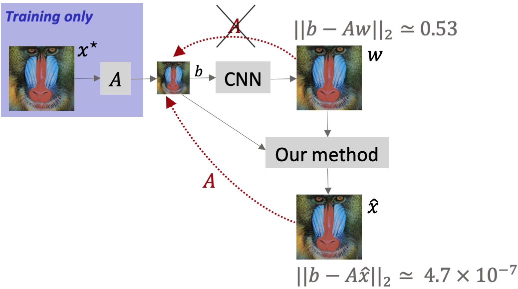
Figure 1: Illustration of the lack of measurement consistency by CNNs during testing: when the output image $w$ is downsampled using $A$, it typically differs significantly from $b$. Our method takes in both $w$ and $b$, and fixes this problem.

Contributions. We summarise our contributions as follows:

1. We introduce a framework that has the advantages of learning-based and reconstruction-based methods. Like reconstruction methods, it is adaptable, flexible, and enforces measurement consistency. At the same time, it retains the excellent performance of learning methods.

2. We integrate learning and reconstruction-based methods via a TV-TV minimization problem. Although we have no specific theoretical guarantees for it, existing theory for a related, simpler problem ($\ell_{1}$-$\ell_{1}$ minimization) provides useful insights about how to tune a regularization parameter. This makes our algorithm easy to deploy, since there are virtually no parameters to tune.

3. We propose an algorithm based on the alternating direction method of multipliers (ADMM) [20] to solve the TV-TV minimization problem. In contrast with most SR methods, which process image patches independently, our algorithm processes full images at once. It also easily adapts to different degradations and scaling factors.

4. We conduct extensive experiments that illustrate not only the robustness of our algorithm under different degradation operators, but also how it systematically improves (in terms of PSNR and SSIM) the outputs of state-of-the-art SR networks, such as ESRGAN [17], VDSR [18] and LapSRN [21].

We highlight the following differences with respect to our previous work in [1, 2]. We now explore and illustrate with experiments the underlying reason why our framework improves the output of state-of-the-art SR CNNs. We also describe how the proposed optimization problem can be solved efficiently using ADMM; in fact, the algorithms used in [1, 2] were different and less efficient than the algorithm we present here. Our experiments are also much more extensive: they consider different sampling operators to illustrate robustness to operator mismatch, and include many more algorithms, e.g., FSRCNN [22], VDSR [18], LapSRN [21], SRMD [23], IRCNN [24], and ESRGAN [17].

Organization. Section II summarizes prior work on SR algorithms, and Section III describes the proposed framework and optimization scheme. Section IV then reports our experimental results, and Section V concludes the paper.

II Related Work

Super-resolution (SR) schemes are often labeled as interpolation, reconstruction, or data-driven. Interpolation methods infer the missing pixels by locally applying an interpolation function such as the bicubic or bilinear filter [3, 4]. As they have been surpassed by both reconstruction and learning SR algorithms, we will limit our review to the latter.

II-A Reconstruction-Based SR

Reconstruction-based schemes view SR as an image reconstruction problem and address it by formulating an optimization problem. In general, the optimization problem has two terms: a data consistency term that encodes assumptions about the acquisition process, usually that $Ax\simeq b$ (where $x$ is the optimization variable), and a regularization term on $x$ that encodes assumptions about the class of images. Different methods differ mostly on the image assumptions.

Image assumptions. Reconstruction SR methods encode assumptions about the images by penalizing in the optimization problem measures of complexity. These reflect the empirical observation that natural images have parsimonious representations in several domains. Examples include sparsity in the wavelet domain [25], sparsity of image patches in the DCT domain [26] and, as we will explore shortly in more detail, sparsity of image gradients [6, 7, 8, 9, 10, 11, 12, 13]. Since sparsity is well captured by the $\ell_{1}$-norm, the resulting optimization problem is typically convex and can be solved efficiently. A more challenging assumption is multi-scale recurrence [27, 28], which captures the notion that patches of natural images occur repeatedly across the image. For example, [27] proposed an SR algorithm that explores the recurrence of image patches both in the same and in different scales.

Total variation. In natural images, the number of pixels that correspond to an edge, i.e., a transition between different objects, is a small percentage of the total number of pixels. This can be measured by the total variation (TV) of the image [6]. Although TV was initially defined in the context of partial differential equations, there has been work that discretizes the differential equations [9, 10] or that directly defines TV in the discrete setting [11, 12, 29]. Although there are several definitions of discrete TV, the most popular are the isotropic TV, which consists of the sum (over all pixels) of the $\ell_{2}$-norms of the vectors containing the horizontal and vertical differences at each pixel, and the anisotropic TV, which is similar to isotropic TV but with the $\ell_{2}$-norms replaced by the $\ell_{1}$-norm. Both definitions yield convex, yet nondifferentiable, functions. Many algorithms have been proposed to solve problems involving discrete TV, including primal-dual methods [30, 8], and proximal and gradient-based schemes [11, 12, 13].

The concept of TV has been used in many imaging tasks, from denoising [6, 11, 29] to super-resolution [9, 11, 10]. For example, [9] discretizes a differential equation relating variations in the values of pixels to the curvature of level sets, while enforcing fidelity to the LR image. The work in [10] proposed a similar method, but with more complex models for both TV and the image acquisition process.

II-B Learning-based Algorithms

Learning-based algorithms typically consist of two stages: training, in which a map from LR to HR patches is learned from a database of training images, and testing, in which the learned map is applied to super-resolve an unseen image.

Manifold learning. Manifold learning relies on the observation that most data (e.g., patches of images) lie on a low-dimensional manifold. An example is locally linear embedding [31] which, like PCA, learns a compact representation of data, but considers nonlinear geometry instead. This idea was applied to SR in [32] by assuming that LR and HR patches lie on manifolds with similar geometry. Thus, given a set of training HR and LR patches and a target LR image, the method in [32] first finds the LR patches in the training set that are neighbors of the target LR patch. Then, it uses the HR version of those neighbors to infer the HR target patches. The resulting algorithm can over- or under-fit the data depending on how many nodes (i.e., patches) define a neighborhood.

Dictionary learning. In dictionary learning, also known as sparse coding, patches of HR images are assumed to have a sparse representation on an over-complete dictionary, which is learned from training images. For example, [14] uses training images to learn dictionaries for LR and HR patches while constraining corresponding patches to have the same coefficients. Other schemes use similar concepts, but require no training data at all. For example, [15] uses self-similarity to learn the LR-HR map without any external database of images.

CNN-based methods. The advent of deep learning and the availability of large image datasets inspired the application of CNNs to SR. Currently, they surpass any reconstruction- or interpolation-based method both in reconstruction performance and in execution time (during testing). The first CNN for SR was proposed by [16]; although its design was inspired by dictionary learning methods, the proposed architecture set a new standard for SR performance.

SR networks can be classified as direct or progressive. In direct networks, the LR image is first upscaled, typically via bicubic interpolation, to the required spatial resolution, and then is fed to a CNN, as in [16, 22, 33, 18]. In this case, the CNN thus learns how to deblur the upscaled image. As previously mentioned, CNN architectures need to be retrained every time we change the scaling factor. To overcome this, [34] repeatedly applied a recursive convolutional layer to obtain the super-resolved image. However, since the LR input is blurry, the CNN outputs a HR image lacking fine details. Inspired by this observation, [35] proposed the SRGAN, which produces photo-realistic HR images, even though they do not yield the best PSNR. As direct networks operate on high-dimensional images, their training is computationally expensive [36].

Progressive networks, in contrast, have reduced training complexity, as they directly process LR images. Specifically, the upsampling step, performed using sub-pixel or transposed convolution [36], is applied only at the end of the network. For instance, LapSRN [21] used the concept of Laplacian pyramids, in which each network level is trained to predict residuals between the upscaled images at different levels in the pyramid. More recently, [37] proposed a fully progressive network that super-resolves images by an upsampling factor of two at each level until the desired factor is reached.

In spite of achieving state-of-the-art performance, CNNs for SR suffer from two major shortcomings: as already illustrated, they fail to guarantee the consistency between the LR and HR image during testing, and the trained network applies only to a unique scaling factor and degradation function. Most of the CNNs, e.g. [16, 22, 23], are trained by solving

$$\underset{\theta}{\text{minimize}}\,\,\,\frac{1}{T}\sum_{t=1}^{T}\big{\|}f_{\theta}(Ax^{(t)})-x^{(t)}\big{\|}_{2}^{2}\,,$$

where $x^{(t)}$ represents (the vectorization of) the $t$th image in the training set, $A$ the bicubic sampling operator, and $f_{\theta}(\cdot)$ a CNN parameterized by $\theta$ (i.e., weights and biases of the neural connections). Most CNNs are trained with images that have been downsampled with a bicubic filter. Thus, their performance quickly degrades when the true downsampling operator is different. Indeed, during testing, the true degradation is unknown. The work in [23] addresses this problem by designing a network that deals with different degradations by accepting as input both the blur kernel and the noise level.

II-C Plug-and-Play Methods

A different line or work blends learning- and model-based methods. The main observation is that, when solving linear inverse problems, proximal-based algorithms separate the operations of measurement consistency and problem regularization (using prior knowledge). The latter usually consists of a simple operation, like soft-thresholding, which encodes the assumptions about the target image and which can be viewed as a denoising step. Given its independence from the measurements, such operation can be replaced by a more complex function, such as a CNN. The resulting algorithms are versatile, as the measurement operator can be easily modified. Most work in this area, however, has focussed on compressed sensing, in which the measurement operator is typically a dense random matrix; see [38, 39, 40].

The One-Net [41], for example, replaces the proximal operator associated to image regularization in an ADMM algorithm with a CNN trained on a large database. The experiments in [41] considered SR, but the resulting network does not perform as well as current leading CNN-based methods.

The pioneering work in [42] takes this idea further and proposes a scheme that requires no training at all. There, an untrained CNN is used as a prior. Specifically, a linear inverse problem is reparameterized as a function of the weights of a CNN whose input is a noisy/corrupted image and whose output is the denoised/reconstructed image. Such reparameterization provides a type of regularization. The work in [43] combined this idea with regularization by denoising and used ADMM to solve the resulting linear inverse problem. See [24, 44] for related work. These algorithms require no training at all and can be easily adapted to different measurement operators. However, they can be particularly slow, as each iteration requires some backpropagation iterations on the CNN. And, when applied to SR, they are still outperformed by training-based CNN architectures.

III Proposed Framework

III-A Main Model and Assumptions

We aim to reconstruct the vectorized version of an HR image $x^{\star}\in\mathbb{R}^{n}$ from a LR image $b\in\mathbb{R}^{m}$, with $m<n$. We assume that these quantities are linearly related:

$$b=Ax^{\star},$$ (1)

where $A\in\mathbb{R}^{m\times n}$ represents the downsampling operator. The model in (1) is often used in reconstruction-based and dictionary learning algorithms [10, 14, 25], even though many methods also consider additive noise: $b=Ax^{\star}+\epsilon$, where $\epsilon$ is a Gaussian random vector [45, 46, 47, 13, 41].

More interesting, however, is that CNN-based methods implicitly assume the model in (1), although that is rarely acknowledged. In particular, all the SR networks we know of (e.g., [16, 21, 22, 17]) are trained with HR images that are downsampled according to (1), where $A$ implements bicubic downsampling. We next discuss other possible choices for $A$.

Common choices for $\boldsymbol{A}$. Different instances of $A\in\mathbb{R}^{m\times n}$ in (1) have been assumed in the SR literature:

• Simple subsampling: $A$ contains equispaced rows of the identity matrix $I_{n}\in\mathbb{R}^{n\times n}$, i.e., each row of $A$ is a canonical vector $(0,...,0,1,0,...,0)$. This operator is simple to implement, but often introduces aliasing.

• Bicubic: $A=S\cdot B$, where $S$ is a simple subsampling operator, and $B$ is a bicubic filter. It is the operator of choice for processing training data for CNNs.

• Box-averaging: if the scaling factor is $s$, then each row of $A$ contains $s^{2}$ nonzero elements, equal to $1/s^{2}$, in positions corresponding to a neighborhood of a pixel. In other words, box-averaging replaces each block of $s\times s$ pixels by their average. Although simpler than the bicubic operator, it does not introduce the aliasing that simple subsampling does; see, e.g., [41].

In our experiments, we will mostly instantiate $A$ as a bicubic operator. The reason is that most SR CNNs assume this operator during training. Simple subsampling and box-averaging will be used to illustrate how our post-processing scheme adds robustness to operator mismatch, i.e., when $A$ is different during training and testing.

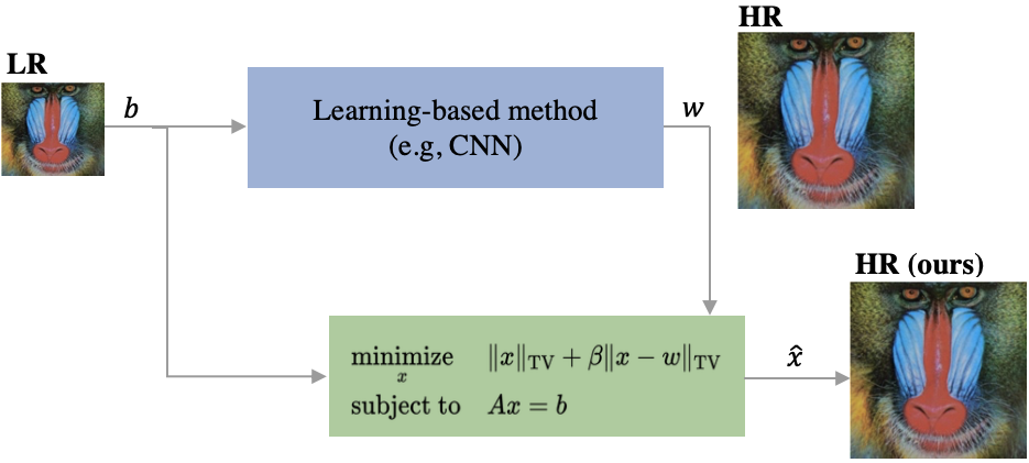
Figure 2: Our framework: the low-resolution image $b$ and the image $w$ super-resolved by a CNN are fed into the TV-TV minimization problem which, in turn, obtains a high-resolution image $\widehat{x}$ with better quality.

Assumptions. We estimate $x^{\star}\in\mathbb{R}^{n}$ from $b\in\mathbb{R}^{m}$ by taking into account two possibly conflicting assumptions:

1. $x^{\star}$ has a small number of edges, as captured by a small total variation (TV);

2. $x^{\star}$ is also close to the side information $w$, the image returned by a learning-based method (CNN), where the notion of distance is also measured by TV.

For a given vectorization $x\in\mathbb{R}^{n}$ of an image $X\in\mathbb{R}^{M\times N}$, the anisotropic 2D TV (semi-)norm is defined as [7, 11]

$$\left\|x\right\|_{\text{TV}}: =\sum_{i=1}^{M}\sum_{j=1}^{N}\left|v_{ij}^{\top}x\right|+\left|h_{ij}^{\top}x\right|\vspace{0.2cm}$$ (2)

$$=\bigg{\|}\begin{bmatrix}V\\ H\end{bmatrix}x\bigg{\|}_{1}\vspace{0.2cm}$$ (3)

$$=\|Dx\|_{1}\,.$$ (4)

In (2), $v_{ij}\in\mathbb{R}^{n}$ and $h_{ij}\in\mathbb{R}^{n}$ extract the vertical and horizontal differences at pixel $(i,j)$ of $X$. By concatenating $v_{ij}$ (resp. $h_{ij}$) as rows of $V\in\mathbb{R}^{n\times n}$ (resp. $H\in\mathbb{R}^{n\times n}$), we obtain the representation in (3), where $\|\cdot\|_{1}$ is the $\ell_{1}$-norm (sum of absolute values). And the matrix $D\in\mathbb{R}^{2n\times n}$ in (4) is the vertical concatenation of $V$ and $H$. We assume periodic boundaries, so that both $V$ and $H$ are circulant. As circulant matrices are diagonalizable by the DFT, matrix-vector products by both $V$ and $H$ can be computed via the FFT in $O(n\log n)$ time.

III-B Our Framework

The framework we propose is shown schematically in Fig. 2. It starts by super-resolving $b$ into $w\in\mathbb{R}^{n}$ with a base method, which we assume is implemented by a CNN due to their current outstanding performance. As explained in Section I, CNNs fail to enforce measurement consistency during testing, i.e., $Aw\neq b$ for any matrix $A$ that is assumed to implement the downsampling operation.

We propose to use an additional block that takes in both the HR output $w$ of the CNN and the LR image $b$, and creates another HR image $\widehat{x}$. The block implements what we call TV-TV minimization, which enforces measurement consistency while guaranteeing that assumptions 1) and 2) are met. This is explained next.

TV-TV minimization. Given the LR image $b$ and a HR image $w$, TV-TV minimization consists of

$$\begin{array}[t]{ll}{\underset{x}{\text{minimize}}}&\|x\|_{\text{TV}}+\beta\|x-w\|_{\text{TV}}\\ \text{subject to}&Ax=b\,,\end{array}$$ (5)

where $x\in\mathbb{R}^{n}$ is the optimization variable, and $\beta\geq 0$ tradeoffs between assumptions 1) and 2). Indeed, the first term in the objective of (5) encodes assumption 1), the second term assumption 2), and the constraints enforce measurement consistency. Of course, our assumptions 1)-2) can be easily modified to better capture the class of images to be super-resolved. We found that using TV semi-norms in the objective yielded better results. In addition, as these functions are convex, problem (5) is convex as well.

Although a problem like (5) has appeared before in [48] in the context of dynamic computed tomography (CT), the side information $w$ there was an image reconstructed by solving the same problem in the previous instant; see also [49, 50, 51]. Our approach is conceptually different in that we use (5) to improve the reconstruction of a CNN-based method.

Next, we show how TV-TV minimization relates to $\ell_{1}$-$\ell_{1}$ minimization, and how the theory for the latter in [49] suggests that selecting $\beta=1$ in (5) may lead to better performance.

Relation to $\ell_{1}$-$\ell_{1}$ minimization. Introducing an auxiliary variable $u\in\mathbb{R}^{2n}$ and defining $\overline{w}:=Dw$, we rewrite (5) as

$$\begin{array}[t]{ll}\underset{u,x}{\text{minimize}}&\|u\|_{1}+\beta\|u-\overline{w}\|_{1}\\ \text{subject to}&Ax=b\\ &Dx=u\,.\end{array}$$ (6)

Thus, $\overline{x}:=(u,x)\in\mathbb{R}^{3n}$ is the full optimization variable. Define $\overline{A}:=\begin{bmatrix}0_{m\times 2n}&A;&-I_{2n}&D\end{bmatrix}$, and $\overline{b}:=\begin{bmatrix}b&0_{2n}\end{bmatrix}^{\top}$, where $0_{a\times b}$ (resp. $0_{a}$) represents the zero matrix (resp. vector) of dimensions $a\times b$ (resp. $a\times 1$), and $I_{2n}$ is the identity matrix in $\mathbb{R}^{2n}$. This enables us to rewrite (6) as

$$\begin{array}[t]{ll}\underset{\overline{x}}{\text{minimize}}&\|G_{2n}\overline{x}\|_{1}+\beta\|G_{2n}\overline{x}-\overline{w}\|_{1}\\ \text{subject to}&\overline{A}\overline{x}=\overline{b}\,,\end{array}$$ (7)

where $G_{2n}\in\mathbb{R}^{2n\times 3n}$ contains the first $2n$ rows of the identity matrix $I_{3n}$. In other words, for a vector $v\in\mathbb{R}^{3n}$, $G_{2n}v$ represents the first $2n$ components of $v$. The work in [49] analyzes (7) when $G_{2n}$ is the full identity matrix and the entries of $\overline{A}$ are drawn from a Gaussian distribution. Specifically, it provides the number of measurements required for perfect reconstruction under these assumptions. It is shown both theoretically and experimentally that the best reconstruction performance is obtained when $\beta=1$. Although the theory in [49] cannot be easily extended to (7), our experiments indicate that $\beta=1$ still leads to the best results in our setting.

III-C Algorithm for TV-TV minimization

We now explain how to efficiently solve TV-TV minimization (5) with the alternating direction method of multipliers (ADMM) [20]. In contrast with the majority of SR algorithms, which operate on individual patches, our algorithm operates on full images. We do that by capitalizing on the fact that matrix-vector multiplications can be performed fast whenever the matrix is $D$ [cf. (2)] or any of the instantiations of $A$ mentioned in Section III-A.

ADMM. The problem that ADMM solves is

$$\begin{array}[t]{ll}\underset{y,z}{\text{minimize}}&f(y)+g(z)\\ \text{subject to}&Fy+Gz=0\,,\end{array}$$ (8)

where $f$ and $g$ are closed, proper, and convex functions, and $F$ and $G$ are given matrices. Associating a dual variable $\lambda$ to the constraints of (8), ADMM iterates on $k$

$$y^{k+1} =\underset{y}{\text{argmin}}\,\,f(y)+\frac{\rho}{2}\big{\|}Fy+Gz^{k}+\lambda^{k}\big{\|}_{2}^{2}$$ (9a)

$$z^{k+1} =\underset{z}{\text{argmin}}\,\,g(z)+\frac{\rho}{2}\big{\|}Fy^{k+1}+Gz+\lambda^{k}\big{\|}_{2}^{2}$$ (9b)

$$\lambda^{k+1} =\lambda^{k}+Fy^{k+1}+Gz^{k+1}\,,$$ (9c)

where $\rho>0$ is the augmented Lagrangian parameter.

Applying ADMM. Although there are many possible reformulations of (5) to which ADMM is applicable, they can yield different performances. Our reformulation simply adds another variable $v\in\mathbb{R}^{n}$ to (6) [which is equivalent to (5)]:

$$\begin{array}[t]{ll}\underset{u,x,v}{\text{minimize}}&\|u\|_{1}+\beta\|u-\overline{w}\|_{1}\\ \text{subject to}&Ax=b\\ &Dv=u\\ &v=x\,.\end{array}$$ (10)

We establish the following correspondence between (8) and (10): we set $y=(u,x)$, $z=v$, and assign

$$f(u,x) =\|u\|_{1}+\beta\|u-\overline{w}\|_{1}+\text{i}_{Ax=b}(x) F =\begin{bmatrix}-I_{2n}&0\\ 0&I_{n}\end{bmatrix}$$

$$g(v) =0 G =\begin{bmatrix}D\\ -I_{n}\end{bmatrix}\,,$$

where $\text{i}_{Ax=b}(x)$ is the indicator function of $Ax=b$, i.e., it evaluates to $0$ if $Ax=b$, and to $+\infty$ otherwise. This means that we dualize only the last two constraints of (10), and thus $\lambda$ has two components: $\lambda=(\eta,\mu)\in\mathbb{R}^{2n}\times\mathbb{R}^{n}$. The above correspondence yields closed-form solutions for the problems in (9a) and (9b) (see below). Furthermore, even though the objective of (10) is not strictly convex, the fact that $F$ and $G$ have full column-rank implies that the sequence $(y^{k},z^{k})$ generated by ADMM (9) has a unique limit point, which solves (10) [52]. We now elaborate on how to solve (9a)-(9b).

Solving (9a). Using the above correspondence, problem (9a) decouples into two independent problems that can be solved in parallel:

$$u^{k+1} =\underset{u}{\text{argmin}}\,\,\,\|u\|_{1}+\beta\|u-\overline{w}\|_{1}+\frac{\rho}{2}\|u-s^{k}\|_{2}^{2}$$ (11)

$$x^{k+1} =\begin{array}[t]{cl}\underset{x}{\text{argmin}}&\frac{1}{2}\|x-p^{k}\|^{2}_{2}\\ \text{s.t.}&Ax=b\,,\end{array}$$ (14)

where we defined $s^{k}:=Dv^{k}+\eta^{k}$ and $p^{k}:=v^{k}-\mu^{k}$.

Problem (11) decomposes further componentwise, and the solution for each component can be obtained by evaluating the respective optimality condition (via subgradient calculus). Namely, for $i=1,\ldots,2n$, if $\overline{w}_{i}\geq 0$, then component $u_{i}^{k+1}$ is given by

$$\left\{\begin{array}[]{ll}s_{i}-\frac{1}{\rho}(\beta+1)&,\,\,s_{i}>\overline{w}_{i}+\frac{1}{\rho}(\beta+1)\vspace{0.1cm}\\ \overline{w}_{i}&,\,\,\overline{w}_{i}-\frac{1}{\rho}(\beta-1)\leq s_{i}\leq\overline{w}_{i}+\frac{1}{\rho}(\beta+1)\vspace{0.1cm}\\ s_{i}+\frac{1}{\rho}(\beta-1)&,\,\,-\frac{1}{\rho}(\beta-1)<s_{i}<\overline{w}_{i}-\frac{1}{\rho}(\beta-1)\vspace{0.1cm}\\ 0&,\,\,-\frac{1}{\rho}(\beta-1)\leq s_{i}\leq-\frac{1}{\rho}(\beta-1)\vspace{0.1cm}\\ s_{i}+\frac{1}{\rho}(\beta+1)&,\,\,s_{1}<-\frac{1}{\rho}(\beta+1)\,.\end{array}\right.$$ (15)

And if $\overline{w}_{i}<0$, then component $u_{i}^{k+1}$ is given by

$$\left\{\begin{array}[]{ll}s_{i}+\frac{1}{\rho}(\beta+1)&,\,\,s_{i}>\frac{1}{\rho}(\beta+1)\vspace{0.1cm}\\ 0&,\,\,\frac{1}{\rho}(\beta-1)\leq s_{i}\leq\frac{1}{\rho}(\beta+1)\vspace{0.1cm}\\ s_{i}-\frac{1}{\rho}(\beta-1)&,\,\,\overline{w}_{i}+\frac{1}{\rho}(\beta-1)<s_{i}<\frac{1}{\rho}(\beta-1)\vspace{0.1cm}\\ \overline{w}_{i}&,\,\,\overline{w}_{i}-\frac{1}{\rho}(\beta+1)\leq s_{i}\leq\overline{w}_{i}+\frac{1}{\rho}(\beta-1)\vspace{0.1cm}\\ s_{i}+\frac{1}{\rho}(\beta+1)&,\,\,s_{i}<\overline{w}_{i}-\frac{1}{\rho}(\beta+1)\,.\end{array}\right.$$ (16)

Problem (14) is the projection of $p^{k}$ onto the solutions of $Ax=b$. Assuming that $A$ has full row-rank, i.e., $AA^{\top}$ is invertible, (14) also has a closed-form solution:

$$x^{k+1}=p^{k}-A^{\top}(AA^{\top})^{-1}(Ap-b)\,,$$ (17)

whose computation has a complexity that depends on the properties of the downsampling operator $A$. When $A$ is simple subsampling or the box-averaging operator, $AA^{\top}$ is the identity matrix $I_{m}$ or a multiple of it. In that case, computing (17) requires only two matrix-vector operations which, due to the structure of $A$, can be implemented by indexing. In other words, there is no need to construct $A$ explicitly.

On the other hand, when $A$ is the bicubic operator, the inverse of $AA^{\top}$ can no longer be computed easily, and we solve the linear system in (17) with the conjugate gradient method. In this case, matrix-vector products can be computed in $O(n\log n)$ time using the FFT.

Solving (9b). With our choice of $g$, $F$, and $G$, problem (9b) becomes

$$v^{k+1} =\underset{v}{\text{argmin}}\,\,\,\frac{1}{2}\big{\|}Dv-u^{k+1}+\eta^{k}\big{\|}_{2}^{2}+\frac{1}{2}\big{\|}v-x^{k+1}+\mu^{k}\big{\|}_{2}^{2}$$

$$=(I_{n}+D^{\top}D)^{-1}\Big{[}x^{k+1}-\mu^{k}+D^{\top}(u^{k+1}-\eta^{k})\Big{]}\,.$$ (18)

Given the definition of $D$ in (3)-(4), we have

$$I_{n}+D^{\top}D =I_{n}+V^{\top}V+H^{\top}H$$

$$=C_{n}^{H}\Big{(}I_{n}+\text{Diag}(C_{n}v)^{2}+\text{Diag}(C_{n}h)^{2}\Big{)}C_{n}\,,$$

where the last step uses the fact that $V$ and $H$ are circulant matrices and, therefore, are generated by some vectors $v$ and $h$, respectively. Also, $C_{n}$ denotes the DFT matrix in $\mathbb{R}^{n}$, and $\text{Diag}(x)$ is a diagonal matrix with the entries of $x$ in its diagonal. This representation of $I_{n}+D^{\top}D$ not only enables us to compute its inverse in closed-form (just take the inverse of the matrix in parenthesis), but also to do it without constructing any matrix explicitly.

Dual updates. Finally, since $\lambda$ decomposes as $(\eta,\mu)$, the dual variable update in (9c) becomes

$$\eta^{k+1} =\eta^{k}+Dv^{k+1}-u^{k+1}$$ (19a)

$$\mu^{k+1} =\mu^{k}+x^{k+1}-v^{k+1}\,.$$ (19b)

Applying ADMM (9) to the equivalent reformulation (10) of TV-TV minimization (5) therefore yields steps (15)-(16) for each component of $u$, (17) for $x$, (18) for $v$, and (19) for the dual variables. These steps are repeated iteratively until a stopping criterion is met; we use the one suggested in [20].

IV Experiments

We now describe our experiments. After explaining the experimental setup, we expand on the phenomenon described in Fig. 1. Then, we consider the case of operator mismatches (i.e., $A$ is different during training and testing), and show how our framework adds significant robustness in this scenario. Finally, we report experiments on standard SR datasets. Code to replicate our experiments is available online.

IV-A Experimental Setup

Algorithm parameters. Most experiments were run using the same algorithm settings, unless indicated otherwise. The hyperparameter $\beta$ in (5) was always set to $1$ and, for most experiments, $A$ was the bicubic operator via MATLAB’s imresize. For ADMM, we adopted the stopping criterion in [20, §3.3.1] with $\epsilon^{\text{pri}}=\epsilon^{\text{dual}}=0.001$, or stopped after $1500$ iterations. Also, we initialized $\rho=0.5$ and adjusted it automatically using the heuristic in [20, §3.4.1].

Datasets. We considered the standard SR test sets Set5 [53], Set14 [54], BSD100 [55] and Urban100 [56], which contain images of animals, buildings, people, and landscapes.

Computational platform. All experiments were run on Matlab (R2019a) using a workstation with 12 core 2.10GHz Intel(R) Xeon(R) Silver 4110 CPU and two Nvidia GeForce RTX GPUs.

Methods evaluated. We compared our framework against the state-of-the-art methods in Table I and also considered simple TV minimization, i.e., (5) with $\beta=0$, using the TVAL3 solver [8]. The table shows the acronyms and references of the methods, their main technique, the scaling factors (S.F.) considered in the original papers, and the datasets used for training. Note that all methods except LapSRN and ESRGAN were evaluated only for $2\times$ and $4\times$ scaling factors. LapSRN also handles an $8\times$ scaling factor, while ESRGAN only handles $4\times$. The training datasets in Table I have 91 (T91), 100 (General100), 200 (BSDS200), 324 (OutdoorSceneTraining), 500 (BSDS500), 800 (DIV2K), 2650 (Flickr2K), 4744 (WED), and 396,000 (ImageNet) images.

TABLE I: METHODS USED IN OUR EXPERIMENTS. FOR EACH, WE SHOW THE MAIN TECHNIQUE, THE SCALING FACTORS IT CAN HANDLE AND, IF ANY, THE TRAINING DATASET.

Method	Type	S.F.	Training dataset
Kim [57]	Regression	2, 4
SRCNN [16]	CNN	2, 4	ImageNet [19]
SelfExSR [56]	Self-similarity	2, 4
FSRCNN [22]	CNN	2, 4	T91 [14], General100 [22]
DRCN [34]	CNN	2, 4	T91 [14]
VDSR [18]	CNN	2, 4	T91 [14], BSDS200 [58]
LapSRN [21]	CNN	2, 4, 8	T91 [14], BSDS200 [58]
SRMD [23]	CNN	2, 4	DIV2K [59], BSDS200 [58]
			WED [60]
IRCNN [24]	Plug-and-play	2, 4	ImageNet [19], WED [60],
			BSDS500 [61]
ESRGAN [17]	GAN	4	DIV2K [59], Flickr2K [62],
			OutdoorSceneTraining [63]
DeepRED [42]	Plug-and-play	2, 4
TVAL3 [8]	Optimization	2, 4

Both during training and testing, all the CNN-based methods in Table I extract the luminance channel of the YCbCr color space, and then convert the image from uint8 to double. During training, the HR images are converted to LR images by applying MATLAB’s imresize, as originally done in [16]. Other methods, such as [64], work on uint8 images directly or use Python’s imresize, which is different from MATLAB’s. To keep our experiments consistent, we did not consider such methods.

The output images for Kim [57], SRCNN [16] and SelfExSR [56] were retrieved from an online repository. For the remaining methods, we generated the outputs from the available pretrained models.

Performance metrics. We compared different algorithms by evaluating the PSNR (dB) and SSIM [65] on the luminance channel of the output images. As these metrics do not often capture perceptual quality, we also provide sample images for qualitative evaluation.

IV-B Measurement Inconsistency of CNNs

We show that the phenomenon illustrated in Fig. 1 for SRCNN [16] occurs not only for this network, but is pervasive. That is, CNNs for SR fail to enforce measurement consistency (1) during testing. We chose three images for this purpose: Baboon from Set14 [54], 38092 from BSD100, and img₀₀₅ from Urban100 [56]. Every image is downsampled with MATLAB’s imresize, which is the procedure executed for training each CNN, and the resulting LR image is fed into the network. We chose a scaling factor of $4$.

Results. Table II shows the results for a subset of methods in Table I. In the 3rd column, it displays the $\ell_{2}$-norm of the difference between the downsampled HR outputs, i.e., $Aw$, and the input LR image $b$; in the 4th column, it shows the same quantity after feeding the corresponding $w$ (and $b$, cf. Fig. 2) to our method. It can be seen our post-processing improves consistency by 6 orders of magnitude. Note that even though SRMD models various degradations without retraining, it still fails to ensure consistency. IRCNN is a plug-and-play method and, as a result, can also handle different degradation models. Although it achieves better consistency than pure CNN-based methods, it is still 5 orders of magnitude below our scheme. The last row of Table II shows the consistency of DeepRED [43], which processes the three RGB channels simultaneously. For this reason, it was difficult to provide a fair comparison with our method.

TABLE II: CONSISTENCY ACHIEVED BY CNN-TYPE METHODS ($\|Aw-b\|_{2}$) AND BY OUR ALGORITHM ($\|A\hat{x}-b\|_{2}$).

Method	Image	$\boldsymbol{\|Aw-b\|_{2}}$	$\boldsymbol{\|A\hat{x}-b\|_{2}}$
SRCNN [16]	Baboon	$\phantom{0}5.29\times 10^{-1}$	$\boldsymbol{4.72\times 10^{-7}}$
	38092	$\phantom{0}5.68\times 10^{-1}$	$\boldsymbol{4.18\times 10^{-7}}$
	img005	$14.93\times 10^{-1}$	$\boldsymbol{7.72\times 10^{-7}}$
FSRCNN [22]	Baboon	$\phantom{0}3.26\times 10^{-1}$	$\boldsymbol{4.81\times 10^{-7}}$
	38092	$\phantom{0}2.91\times 10^{-1}$	$\boldsymbol{3.80\times 10^{-7}}$
	img005	$10.32\times 10^{-1}$	$\boldsymbol{3.55\times 10^{-7}}$
SRMD [23]	Baboon	$\phantom{0}4.14\times 10^{-1}$	$\boldsymbol{6.62\times 10^{-7}}$
	38092	$\phantom{0}2.39\times 10^{-1}$	$\boldsymbol{9.48\times 10^{-7}}$
	img005	$\phantom{0}9.53\times 10^{-1}$	$\boldsymbol{9.89\times 10^{-7}}$
IRCNN [24]	Baboon	$\phantom{0}8.72\times 10^{-2}$	$\boldsymbol{5.42\times 10^{-7}}$
	38092	$\phantom{0}8.06\times 10^{-2}$	$\boldsymbol{4.08\times 10^{-7}}$
	img005	$\phantom{0}4.57\times 10^{-1}$	$\boldsymbol{6.70\times 10^{-7}}$
DeepRed [43]	Baboon	$\phantom{0}2.62\times 10^{-1}$
	38092	$\phantom{0}2.06\times 10^{-1}$
	img005	$\phantom{0}3.11\times 10^{-1}$

TABLE III: OPERATOR MISMATCH EXPERIMENTS. PSNR VALUES UNDER DIFFERENT SAMPLING OPERATORS FOR $A$: BICUBIC, BOX FILTERING, AND SIMPLE SUBSAMPLING. WITHIN EACH BOX, THE BEST (HIGHER) VALUES ARE HIGHLIGHTED IN BOLD.

Method	Image	Bic.	Ours	Box	Ours	Sub.	Ours
SRCNN [16]	Baboon	22.70	22.73	22.49	22.53	17.48	19.31
	38092	25.90	25.95	25.69	25.77	20.07	21.98
	img005	25.12	25.28	24.99	25.24	17.92	19.91
FSRCNN [22]	Baboon	22.79	22.80	22.49	22.56	17.38	19.45
	38092	26.03	26.06	25.64	25.74	20.00	22.05
	img005	25.81	25.87	25.12	25.38	17.79	19.85
SRMD [23]	Baboon	22.90	22.91	22.52	22.61	16.95	19.21
	38092	26.20	26.21	25.62	25.74	19.39	21.70
	img005	26.56	26.60	25.59	25.96	17.36	19.58
IRCNN [24]	Baboon	22.76	22.76	22.51	22.51	17.41	19.59
	38092	26.09	26.09	25.77	25.78	20.54	22.53
	img005	26.18	26.20	25.86	25.86	18.23	19.83
TVAL3 [8]	Baboon	22.40		22.27		20.83
	38092	25.59		25.00		21.35
	img005	24.29		22.54		17.28

IV-C Robustness to Operator Mismatch

As previously stated, most SR CNNs are trained by downsampling a HR into a LR image using the bicubic operator. If, during testing, $A$ is different from the bicubic operator then, as we will see, there can be a serious drop in performance. This may indeed limit the applicability of CNNs in real-life scenarios. Our approach, however, mitigates this effect and adds robustness to the SR task. We considered the same images and methods as in Table II, with DeepRed replaced by TVAL3, and considered the operators for $A$ described in Section III-A: bicubic, box averaging, and simple subsampling.

Results. Each shaded box in Table III shows, for each subsampling operator, the PSNR values obtained by a given method, and by subsequently processing its output with our scheme. While all methods perform the best under bicubic subsampling, there is a performance drop for box filtering, and an even larger drop for simple subsampling. Note that our method systematically improves the output of all the networks, even for bicubic subsampling. And while the improvement is of less than 1dB for bicubic subsampling, it averages around 2dBs for simple subsampling. Indeed, the performance of the CNNs for this case drops so much that there is a large margin for improvement. Interestingly, TVAL3, which solves (5) with $\beta=0$, is the worst method for bicubic subsampling, but approaches the performance of CNNs for box averaging and, besides ours, becomes the best for simple subsampling. Hence, this illustrates that reconstruction-based methods can be more robust and adaptable than CNN architectures.

TABLE IV: AVERAGE PSNR (SSIM) RESULTS IN dB AND EXECUTION TIME IN SECONDS OF OUR METHOD USING THE REFERENCE METHODS.

Dataset	Scale	TVAL3 [8]	Kim [57]	Ours	Time	SRCNN [16]	Ours	Time
Set5	$\times 2$	34.0315 (0.9354)	36.2465 (0.9516)	36.4499 (0.9537)	61.89	36.2772 (0.9509)	36.5288 (0.9536)	56.60
	$\times 4$	29.1708 (0.8349)	30.0730 (0.8553)	30.2289 (0.8593)	46.96	30.0765 (0.8525)	30.2669 (0.8590)	46.93
Set14	$\times 2$	31.0033 (0.8871)	32.1359 (0.9031)	32.3044 (0.9055)	58.99	31.9954 (0.9012)	32.2949 (0.9057)	57.86
	$\times 4$	26.6742 (0.7278)	27.1836 (0.7434)	27.2993 (0.7488)	42.87	27.1254 (0.7395)	27.3040 (0.7480)	41.79
BSD100	$\times 2$	30.1373 (0.8671)	31.1124 (0.8840)	31.2097 (0.8864)	26.40	31.1087 (0.8835)	31.2241 (0.8866)	27.13
	$\times 4$	26.3402 (0.6900)	26.7099 (0.7027)	26.7891 (0.7086)	16.72	26.7027 (0.7018)	26.7838 (0.7085)	16.90
Urban100	$\times 2$	27.5143 (0.8728)	28.7415 (0.8940)	28.8901 (0.8953)	37.16	28.6505 (0.8909)	28.8415 (0.8939)	30.56
	$\times 4$	23.7529 (0.6977)	24.1968 (0.7104)	24.2778 (0.7147)	215.76	24.1443 (0.7047)	24.2368 (0.7114)	210.74
Dataset	Scale	TVAL3 [8]	SelfExSR [56]	Ours	Time	FSRCNN [22]	Ours	Time
Set5	$\times 2$	34.0315 (0.9354)	36.5001 (0.9537)	36.5321 (0.9542)	61.90	36.9912 (0.9556)	37.0394 (0.9559)	68.97
	$\times 4$	29.1708 (0.8349)	30.3317 (0.8623)	30.3370 (0.8625)	44.66	30.7122 (0.8658)	30.8005 (0.8691)	50.29
Set14	$\times 2$	31.0033 (0.8871)	32.2272 (0.9036)	32.3951 (0.9059)	57.24	32.6515 (0.9089)	32.6935 (0.9092)	67.49
	$\times 4$	26.6742 (0.7278)	27.4014 (0.7518)	27.4730 (0.7536)	39.79	27.6179 (0.7550)	27.6890 (0.7574)	52.47
BSD100	$\times 2$	30.1373 (0.8671)	31.1833 (0.8855)	31.2056 (0.8862)	27.00	31.5075 (0.8905)	31.5250 (0.8907)	26.50
	$\times 4$	26.3402 (0.6900)	26.8459 (0.7108)	26.8482 (0.7108)	16.25	26.9675 (0.7130)	27.0011 (0.7149)	20.76
Urban100	$\times 2$	27.5143 (0.8728)	29.3785 (0.9032)	29.4578 (0.9035)	298.04	29.8734 (0.9010)	29.8926 (0.9013)	263.39
	$\times 4$	23.7529 (0.6977)	24.8241 (0.7386)	24.8315 (0.7385)	203.47	24.6196 (0.7270)	24.6619 (0.7297)	203.82
Dataset	Scale	TVAL3 [8]	DRCN [34]	Ours	Time	VDSR [18]	Ours	Time
Set5	$\times 2$	34.0315 (0.9354)	37.6279 (0.9588)	37.6712 (0.9591)	57.23	37.5295 (0.9587)	37.5669 (0.9588)	65.91
	$\times 4$	29.1708 (0.8349)	31.5344 (0.8854)	31.5701 (0.8858)	46.66	31.3485 (0.8838)	31.3780 (0.8840)	47.59
Set14	$\times 2$	31.0033 (0.8871)	33.0585 (0.9121)	33.1038 (0.9129)	55.65	33.0527 (0.9127)	33.1058 (0.9131)	62.57
	$\times 4$	26.6742 (0.7278)	28.0269 (0.7673)	28.0588 (0.7680)	42.57	28.0152 (0.7678)	28.0487 (0.7684)	53.32
BSD100	$\times 2$	30.1373 (0.8671)	31.8536 (0.8942)	31.8737 (0.8953)	26.46	31.9015 (0.8960)	31.9142 (0.8962)	26.92
	$\times 4$	26.3402 (0.6900)	27.2364 (0.7233)	27.2524 (0.7240)	19.17	26.8776 (0.7093)	27.2535 (0.7238)	20.74
Dataset	Scale	TVAL3 [8]	LapSRN [21]	Ours	Time	SRMD [23]	Ours	Time
Set5	$\times 2$	34.0315 (0.9354)	37.7008 (0.9590)	37.7219 (0.9592)	62.45	37.4496 (0.9579)	37.5817 (0.9585)	74.33
	$\times 4$	29.1708 (0.8349)	31.7181 (0.8891)	31.7428 (0.8894)	45.19	31.5750 (0.8853)	31.6531 (0.8863)	58.01
	$\times 8$	24.9663 (0.6722)	26.3314 (0.7548)	26.3881 (0.7545)	50.01
Set14	$\times 2$	31.0033 (0.8871)	33.2518 (0.9138)	33.2709 (0.9142)	56.65	33.1035 (0.9127)	33.1868 (0.9137)	69.58
	$\times 4$	26.6742 (0.7278)	28.2533 (0.7730)	28.2722 (0.7734)	42.04	28.1593 (0.7716)	28.2174 (0.7728)	52.03
	$\times 8$	23.6079 (0.5800)	24.5643 (0.6266)	24.5993 (0.6264)	42.48
BSD100	$\times 2$	30.1373 (0.8671)	32.0214 (0.8970)	32.0274 (0.8975)	24.53	31.8722 (0.8953)	31.9009 (0.8959)	28.15
	$\times 4$	26.3402 (0.6900)	27.4164 (0.7296)	27.4317 (0.7300)	19.03	27.3350 (0.7273)	27.3579 (0.7280)	20.94
	$\times 8$	23.9971 (0.5542)	24.6495 (0.5887)	24.6769 (0.5886)	18.30
Urban100	$\times 2$	27.9935 (0.8742)	31.1319 (0.9180)	31.1462 (0.9183)	259.22	30.8799 (0.9146)	30.9253 (0.9151)	266.98
	$\times 4$	23.7529 (0.6977)	25.5026 (0.7661)	25.5167 (0.7662)	199.70	25.3494 (0.7605)	25.3834 (0.7609)	209.77
	$\times 8$	21.1208 (0.5357)	22.0547 (0.5956)	22.0675 (0.5944)	178.60
Dataset	Scale	TVAL3 [8]	IRCNN [24]	Ours	Time	ESRGAN [17]	Ours	Time
Set5	$\times 2$	34.0315 (0.9354)	37.3436 (0.9572)	37.3684 (0.9576)	67.03
	$\times 4$	29.1708 (0.8349)	30.9995 (0.8778)	31.0041 (0.8779)	52.06	32.7072 (0.9001)	32.7170 (0.9002)	44.33
Set14	$\times 2$	31.0033 (0.8871)	32.8573 (0.9105)	32.8929 (0.9110)	65.13
	$\times 4$	26.6742 (0.7278)	27.7195 (0.7614)	27.7420 (0.7615)	52.36	28.8342 (0.7877)	28.9253 (0.7891)	42.40
BSD100	$\times 2$	31.0033 (0.8871)	31.6543 (0.8918)	31.6723 (0.8923)	25.04
	$\times 4$	26.3402 (0.6900)	27.0848 (0.7188)	27.0922 (0.7189)	20.79	27.8332 (0.7447)	27.8489 (0.7447)	19.05
Urban100	$\times 2$	31.0033 (0.8871)	30.0623 (0.9105)	30.0806 (0.9108)	74.41
	$\times 4$	23.7529 (0.6977)	24.8913 (0.7395)	24.9007 (0.7396)	212.49	27.0270 (0.8146)	27.0404 (0.8146)	206.61

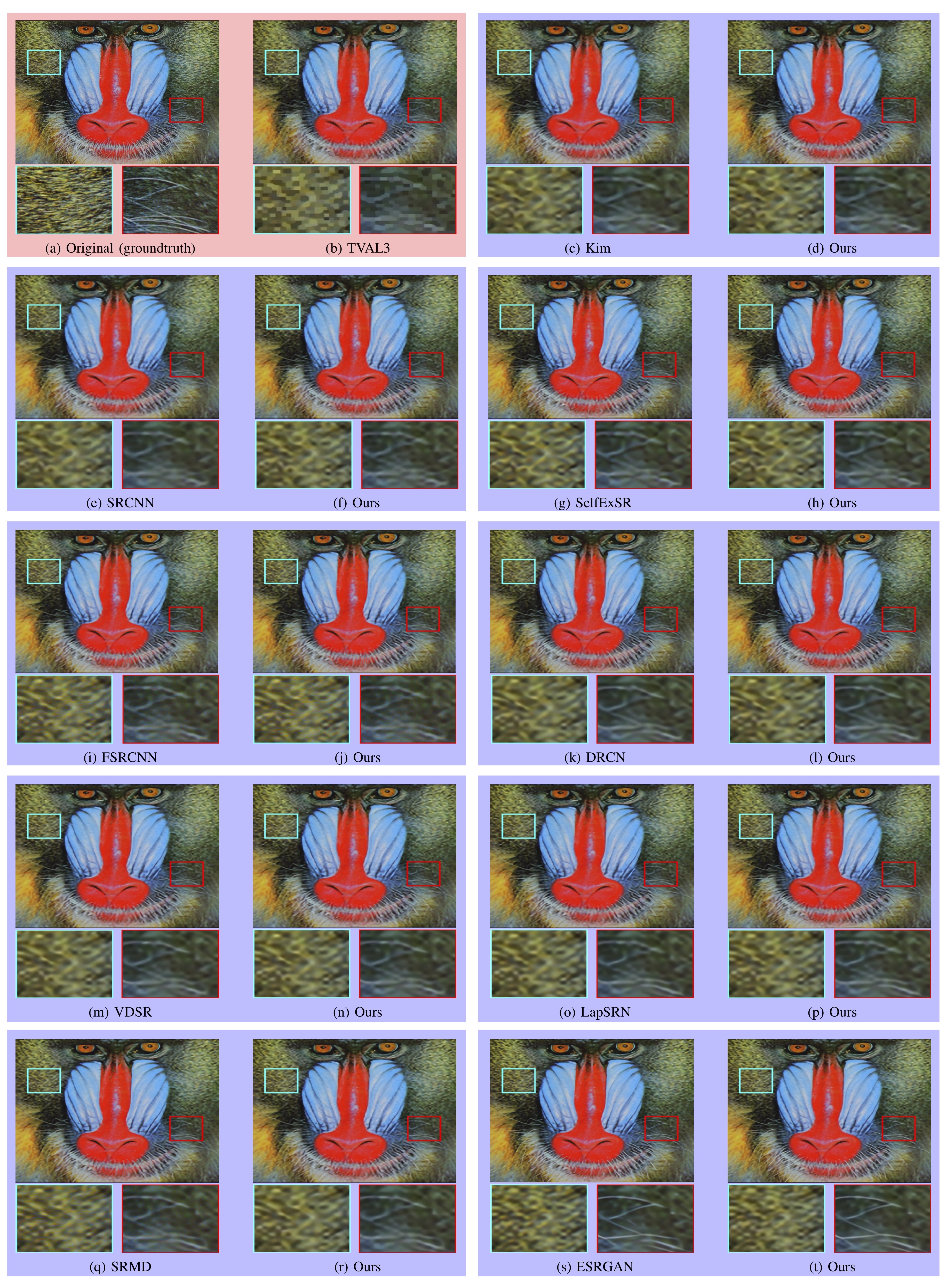
Figure 3: Results on Baboon (Set14) for $4\times$. Each shaded area (except the top-left) shows the output of a learning-based algorithm and of our method.

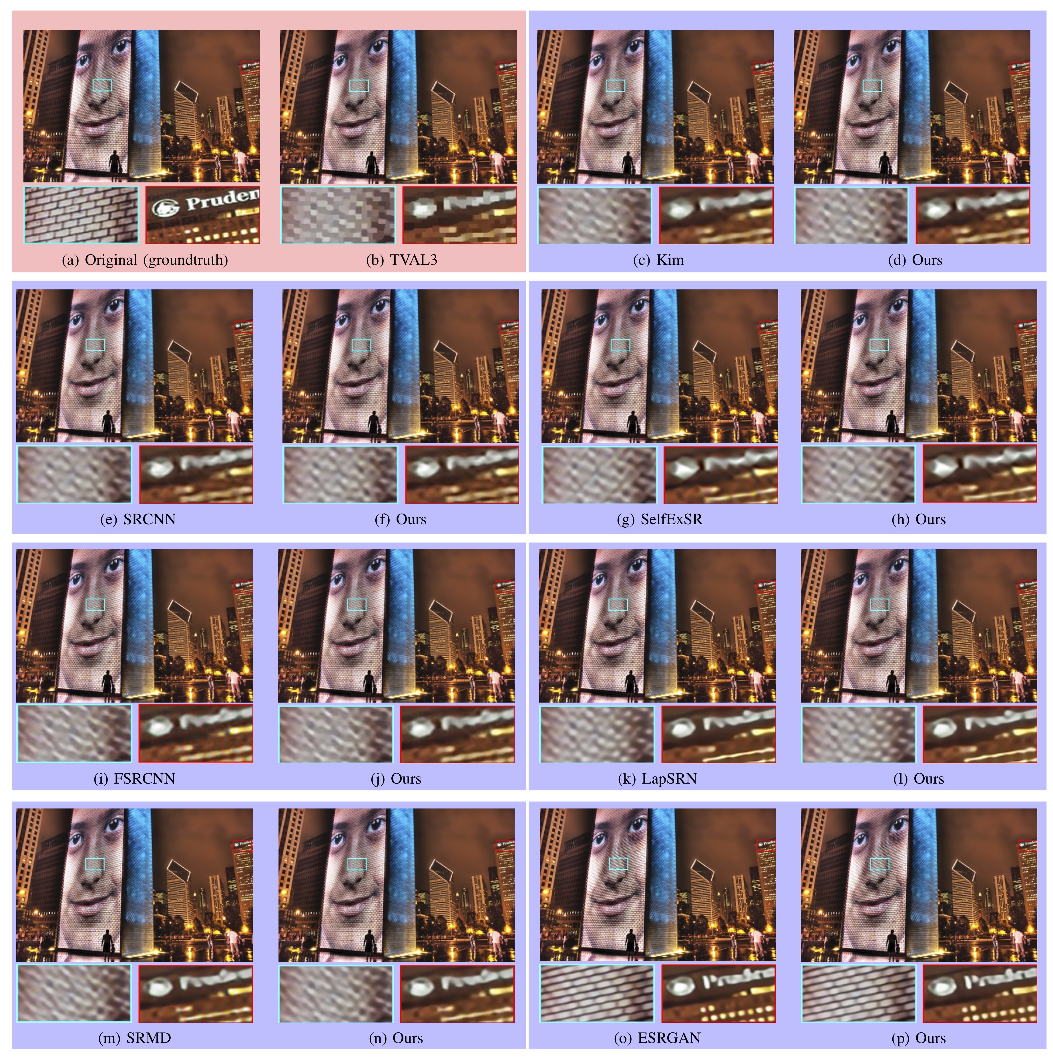
Figure 4: Results on img076 image from Urban100 for $4\times$. Each shaded area (except the top-left) shows the output of a learning-based algorithm and of our method.

IV-D Standard Datasets With Bicubic Downsampling

We also conducted more systematic experiments using the standard datasets Set5, Set14, BSD100, and Urban100, under different scaling factors and using bicubic downsampling only.

Quantitative results. Table IV displays the average PSNR and SSIM, as well as the average execution time of our method (in seconds), for $2\times$, $4\times$, and $8\times$ scaling factors. Each shaded area shows the performance of a given (learning-based) reference method, the performance of our scheme applied to the output of that reference method, and the average execution time (of our method). For easy comparison, the values for TVAL3 occur repeatedly in different vertical sub-blocks of the table. Note that the 4th vertical sub-block of the table is the only one with values for $8\times$ upsampling, since LapSRN is the only method that can handle such a scaling factor. Also, as ESRGAN was designed specifically for $4\times$ upsampling, we do not present its values for other scaling factors. All results for our method were generated with $\beta=1$ in (5), except when we considered LapSRN and ESRGAN for the Urban100 dataset, in which case we set $\beta=2$.

An obvious pattern in the table is that our method consistently improves the outputs of all the methods in terms of PSNR and SSIM, except in a small subset of cases. The improvements range between 0.0023 and 0.3796 dB. One of the exceptions occurs for $8\times$ upsampling with LapSRN. In that case, LapSRN has always better SSIM than our method, even though the opposite happens for the PSNR. As expected, TVAL3 had the worst performance overall and was surpassed by all learning-based methods.

A drawback of our method, however, is its possibly long execution time. We recall that of all downsampling operators mentioned in Section III-A, the most computationally complex is bicubic downsampling, as considered in these experiments. The timing values in Table IV are average values: they report the total execution time of our algorithm over all the images of the corresponding dataset divided by the number of images. While in some cases our algorithm took an average of 16 sec (SRCNN, BSD100, $4\times$), in others it took more than 250 sec (LapSRN, Urban100, $2\times$). In fact, for the Urban100 dataset, because of the large size of its images ($1024\times 644$), we had to reduce the number of simultaneous threads to prevent the GPUs from overflowing. For reference, for (SRCNN, BSD100, $4\times$), our method takes an average of 9 sec when we use simple subsampling. This is roughly half the execution time it takes for bicubic downsampling.

Qualitative results. Figures 3 and 4 depict the output images of all the algorithms (except IRCNN) for the test images baboon from Set14, and img067 from Urban100. All super-resolved images exhibit blur and loss of information compared with the groundtruth images in Figs. LABEL:SubFig:baboonGT-LABEL:SubFig:076GT. And as our scheme builds upon the outputs of other methods, it also inherits some of their artifacts. It is difficult to visually assess differences between the outputs of the algorithms and of our method, in part because the improvements, as measured by the PSNR, are relatively small. Yet, as our experiments show, our scheme not only systematically improves the outputs of CNN-based methods, but also adds significant robustness to operator mismatch.

V Conclusions

We proposed a framework for single-image super-resolution that blends model- and learning-based (e.g., CNN) techniques. As a result, our framework enables solving the consistency problem that CNNs suffer from, namely that downsampled output (HR) images fail to match the input (LR) images. Our experiments show that enforcing such consistency not only systematically improves the quality of the output images of CNNs, but also adds robustness to the super-resolution task. At the core of our framework is a problem that we call TV-TV minimization and which we solve with an ADMM-based algorithm. Although our implementation is efficient, there is still margin to improve its execution time, for example, by unrolling the proposed algorithm with a neural network. We leave this for future work.

References

- [1] M. Vella and J. F. C. Mota, “Single image super-resolution via CNN architectures and TV-TV minimization,” in Proc. BMVC, 2019.
- [2] M. Vella and J. F. C. Mota, “Robust super-resolution via deep learning and TV priors,” in in Proc. SPARS, 2019.
- [3] T. Blu, P. Thevenaz, and M. Unser, “Linear interpolation revitalized,” IEEE Trans. on Image Process., vol. 13, no. 5, pp. 710–719, 2004.
- [4] R. G. Keys, “Cubic convolution interpolation for digital image processing,” IEEE Trans. on Acoust. Speech and Signal Process., vol. 29, no. 6, pp. 1153–1160, 1981.
- [5] R. Fattal, “Image upsampling via imposed edge statistics,” ACM Trans. Graphics, vol. 26, no. 3, 2007.
- [6] S. Osher and L. Rudin, “Feature-oriented image enhancement using shock filters,” SIAM J. Numer. Anal., vol. 27, no. 4, pp. 919–940, 1990.
- [7] L. I. Rudin, S. Osher, and E. Fatemi, “Nonlinear total variation based noise removal algorithms,” Physica D, vol. 60, pp. 259–268, 1992.
- [8] C. Li, W. Yin, H. Jiang, and Y. Zhang, “An efficient augmented lagrangian method with applications to total variation minimization,” J. Comput. Optim. and Appl., vol. 56, no. 3, pp. 507–530, 2013.
- [9] B. S. Morse and D. Schwartzwald, “Image magnification using level set reconstruction,” in Proc. CVPR, 2001, pp. 333–334.
- [10] H. A. Aly and E. Dubois, “Image up-sampling using total-variation regularization with a new observation model,” IEEE Trans. on Image Process., vol. 14, no. 10, pp. 1647–1659, 2005.
- [11] A. Chambolle, “An algorithm for total variation minimization and applications,” J. Math. Imaging Vision, vol. 20, no. 1, pp. 89–97, 2004.
- [12] J. M. Bioucas-Dias and M. A. T. Figueiredo, “A new TwIST: Two-step iterative shrinkage/thresholding algorithms for image restoration,” IEEE Trans. on Image Process., vol. 16, no. 12, pp. 2992–3004, 2007.
- [13] S. Becker, J. Bobin, and E. Candès, “NESTA: a fast and accurate first-order method for sparse recovery,” SIAM J. Imaging Sci., vol. 4, no. 1, pp. 1–39, 2011.
- [14] J. Yang, J. Wright, T. S. Huang, and Y. Ma, “Image super-resolution via sparse representation,” IEEE Trans. on Image Process., vol. 19, no. 11, pp. 2861–2873, 2010.
- [15] A. Singh, F. Porikli, and N. Ahuja, “Super-resolving noisy images,” in Proc. CVPR, 2014, pp. 2846–2853.
- [16] C. Dong, C. C. Loy, K. He, and X. Tang, “Learning a deep convolutional network for image super-resolution,” in Proc. ECCV, 2014, pp. 184–199.
- [17] X. Wang, K. Yu, S. Wu, J. Gu, Y. Liu, C. Dong, Y. Qiao, and C. C. Loy, “ESRGAN: Enhanced super-resolution generative adversarial networks,” in Proc. ECCVW, 2018.
- [18] J. Kim, J. Lee, and K. Lee, “Accurate image super-resolution using very deep convolutional networks,” in Proc. CVPR, 2016, pp. 1646–1654.
- [19] J. Deng, W. Dong, R. Socher, L. jia Li, K. Li, and L. Fei-fei, “ImageNet: A large-scale hierarchical image database,” in Proc. CVPR, 2009.
- [20] S. Boyd, N. Parikh, E. Chu, B. Peleato, and J. Eckstein, “Distributed optimization and statistical learning via the alternating method of multipliers,” Foundations and Trends in Machine Learning, vol. 3, no. 1, pp. 1–122, 2011.
- [21] W.-S. Lai, J.-B. Huang, N. Ahuja, and M.-H. Yang, “Deep laplacian pyramid networks for fast and accurate super-resolution,” in Proc. CVPR, 2017.
- [22] C. Dong, C. C. Loy, and X. Tang, “Accelerating the super-resolution convolutional neural network,” in Proc. ECCV, 2016.
- [23] K. Zhang, W. Zuo, and L. Zhang, “Learning a single convolutional super-resolution network for multiple degradations,” in Proc. CVPR, 2018, pp. 3262–3271.
- [24] K. Zhang, W. Zuo, S. Gu, and L. Zhang, “Learning deep CNN denoiser prior for image restoration,” in Proc. CVPR, 2017, pp. 3929–3938.
- [25] S. Mallat and G. Yu, “Super-resolution with sparse mixing estimators,” IEEE Trans. on Image Process., vol. 19, no. 11, pp. 2889–2900, 2010.
- [26] W. Zhang and W. Cham, “Hallucinating face in the DCT domain,” IEEE Trans. on Image Process., vol. 20, no. 10, pp. 2769–2779, 2011.
- [27] D. Glasner, S. Bagon, and M. Irani, “Super-resolution from a single image,” in Proc. ICCV, 2009, pp. 349–356.
- [28] B. Lim, S. Son, H. Kim, S. Nah, and K. Mu Lee, “Enhanced deep residual networks for single image super-resolution,” in Proc. CVPRW, 2017.
- [29] L. Condat, “Discrete total variation: New definition and minimization,” vol. 10, no. 3, pp. 1258–1290, 2017.
- [30] T. Goldstein and S. Osher, “The split Bregman method for L1-regularized problems,” SIAM J. Imaging Science, vol. 2, no. 2, pp. 323–343, 2009.
- [31] S. T. Roweis and L. K. Saul, “Nonlinear dimensionality reduction by locally linear embedding,” Science, vol. 290, no. 5500, pp. 2323–2326, 2000.
- [32] H. Chang, D. Yueng, and Y. Xiong, “Super-resolution through neighbor embedding,” in Proc. CVPR, vol. 1, 2004, pp. 275–282.
- [33] T. Tong, G. Li, X. Liu, and Q. Gao, “Image super-resolution using dense skip connections,” in Proc. ICCV, 2017, pp. 4809–4817.
- [34] J. Kim, J. Lee, and K. Lee, “Deeply-recursive convolutional network for image super-resolution,” in Proc. CVPR, 2016, pp. 1637–1645.
- [35] C. Ledig, L. Theis, F. Huszár, J. Caballero, A. Cunningham, A. Acosta, A. Aitken, A. Tejani, J. Totz, Z. Wang, and W. Shi, “Photo-realistic single image super-resolution using a generative adversarial network,” in Proc. CVPR, 2017, pp. 105–114.
- [36] W. Shi, J. Caballero, F. Huszár, J. Totz, A. P. Aitken, R. Bishop, D. Rueckert, and Z. Wang, “Real-time single image and video super-resolution using an efficient sub-pixel convolutional neural network,” Proc. CVPR, pp. 1874–1883, 2016.
- [37] Y. Wang, F. Perazzi, B. McWilliams, A. Sorkine-Hornung, O. Sorkine-Hornung, and C. Schroers, “A fully progressive approach to single-image super-resolution,” in Proc. CVPRW, 2018.
- [38] J. Zhang and B. Ghanem, “ISTA-Net: Interpretable optimization-inspired deep network for image compressive sensing,” in Proc. CVPR, 2018, pp. 1828–1837.
- [39] K. Kulkarni, S. Lohit, P. Turaga, R. Kerviche, and A. Ashok, “ReconNet: Non-iterative reconstruction of images from compressively sensed measurements,” in Proc. CVPR, 2016, pp. 449–458.
- [40] A. Bora, A. Jalal, E. Price, and A. G. Dimakis, “Compressed sensing using generative models,” in Proc. ICML, 2017.
- [41] J. H. R. Chang, C. Li, B. Poczos, B. V. K. V. Kumar, and A. C. Sankaranarayanan, “One network to solve them all? solving linear inverse problems using deep projection models,” in Proc. ICCV), 2017, pp. 5889–5898.
- [42] U. Dmitry, V. Andrea, and L. Victor, “Deep image prior,” in Proc. CVPR, 2017.
- [43] G. Mataev, P. Milanfar, and M. Elad, “DeepRED: Deep Image Prior Powered by RED,” in Proc. ICCVW, 2019.
- [44] D. Geman and Chengda Yang, “Nonlinear image recovery with half-quadratic regularization,” IEEE Trans. on Image Process., vol. 4, no. 7, pp. 932–946, 1995.
- [45] F. Shi, J. Cheng, L. Wang, P. Yap, and D. Shen, “LRTV: MR image super-resolution with low-rank and total variation regularizations,” IEEE Trans. on Med. Imaging, vol. 34, no. 12, pp. 2459–2466, 2015.
- [46] J. Li, J. Wu, H. Deng, and J. Liu, “A self-learning image super-resolution method via sparse representation and non-local similarity,” Neurocomputing, vol. 184, pp. 196–206, 2016.
- [47] G. Peyré, S. Bougleux, and L. Cohen, “Non-local regularization of inverse problems,” in Proc. ECCV, 2008, pp. 57–68.
- [48] G.-H. Chen, J. Tang, and S. Leng, “Prior image constrained compressed sensing (PICCS): a method to accurately reconstruct dynamic CT images from highly undersampled projection data sets,” J. Med. Phys., vol. 35, no. 2, pp. 660–663, 2008.
- [49] J. F. C. Mota, N. Deligiannis, and M. R. D. Rodrigues, “Compressed sensing with prior information: Strategies, geometry, and bounds,” IEEE Trans. on Inf. Theory, vol. 63, no. 7, pp. 4472–4496, 2017.
- [50] L. Weizman, Y. C. Eldar, and D. Ben-Bashat, “Reference-based MRI,” J. Med. Phys., vol. 43, no. 10, pp. 5357–5369, 2016.
- [51] J. F. C. Mota, N. Deligiannis, A. C. Sankaranarayanan, V. Cevher, and M. R. D. Rodrigues, “Adaptive-rate reconstruction of time-varying signals with application in compressive foreground extraction,” IEEE Trans. on Signal Process., vol. 64, no. 14, pp. 3651–3666, 2016.
- [52] J. F. C. Mota, J. M. F. Xavier, P. M. Q. Aguiar, and M. Püschel. (2011) A proof of convergence for the alternating direction method of multipliers applied to polyhedral-constrained functions.
- [53] M. Bevilacqua, A. Roumy, C. Guillemot, and M. L. A. Morel, “Low-complexity single-image super-resolution based on nonnegative neighbor embedding,” in Proc. BMVC, 2012, pp. 135.1–135.10.
- [54] R. Zeyde, M. Elad, and M. Protter, “On single image scale-up using sparse-representations,” in Curves and Surfaces, 2012, pp. 711–730.
- [55] D. Martin, C. Fowlkes, D. Tal, and J. Malik, “A database of human segmented natural images and its application to evaluating segmentation algorithms and measuring ecological statistics,” in Proc. ICCV, vol. 2, 2001, pp. 416–423.
- [56] J. Huang, A. Singh, and N. Ahuja, “Single image super-resolution from transformed self-exemplars,” in Proc. CVPR, 2015, pp. 5197–5206.
- [57] K. I. Kim and Y. Kwon, “Single-image super-resolution using sparse regression and natural image prior,” IEEE Trans. Pattern Anal. Mach. Intell., vol. 32, no. 6, pp. 1127–1133, 2010.
- [58] P. Arbeláez, M. Maire, C. Fowlkes, and J. Malik, “Contour detection and hierarchical image segmentation,” IEEE Trans. Pattern Anal. Mach. Intell., vol. 33, no. 5, pp. 898–916, 2011.
- [59] E. Agustsson and R. Timofte, “NTIRE challenge on single image super-resolution: Dataset and study,” Proc. CVPRW, pp. 1122–1131, 2017.
- [60] K. Ma, Z. Duanmu, Q. Wu, Z. Wang, H. Yong, H. Li, and L. Zhang, “Waterloo exploration database: New challenges for image quality assessment models,” IEEE Trans. on Image Process., vol. 26, no. 2, pp. 1004–1016, 2017.
- [61] P. Arbeláez, M. Maire, C. Fowlkes, and J. Malik, “Contour detection and hierarchical image segmentation,” IEEE Trans. Pattern Anal. Mach. Intell., vol. 33, no. 5, pp. 898–916, 2011.
- [62] R. Timofte, E. Agustsson, L. Van Gool, M. Yang, L. Zhang, B. Lim, S. Son, H. Kim, S. Nah, and K. Lee, “NTIRE challenge on single image super-resolution: Methods and results,” in Proc. CVPRW, 2017, pp. 1110–1121.
- [63] X. Wang, K. Yu, C. Dong, and C. C. Loy, “Recovering realistic texture in image super-resolution by deep spatial feature transform,” in Proc. CVPR, 2018.
- [64] Y. Zhang, K. Li, K. Li, L. Wang, B. Zhong, and Y. Fu, “Image super-resolution using very deep residual channel attention networks,” in Proc. ECCV, 2018.
- [65] Z. Wang, A. C. Bovik, H. R. Sheikh, and E. P. Simoncelli, “Image quality assessment: from error visibility to structural similarity,” IEEE Trans. on Image Process., vol. 13, no. 4, pp. 600–612, 2004.