Efficient Online Classification and Tracking on Resource-constrained IoT Devices

Abstract.

Timely processing has been increasingly required on smart IoT devices, which leads to directly implementing information processing tasks on an IoT device for bandwidth savings and privacy assurance. Particularly, monitoring and tracking the observed signals in continuous form are common tasks for a variety of near real-time processing IoT devices, such as in smart homes, body-area and environmental sensing applications. However, these systems are likely low-cost resource-constrained embedded systems, equipped with compact memory space, whereby the ability to store the full information state of continuous signals is limited. Hence, in this paper^∗ we develop solutions of efficient timely processing embedded systems for online classification and tracking of continuous signals with compact memory space. Particularly, we focus on the application of smart plugs that are capable of timely classification of appliance types and tracking of appliance behavior in a standalone manner. We implemented a smart plug prototype using low-cost Arduino platform with small amount of memory space to demonstrate the following timely processing operations: (1) learning and classifying the patterns associated with the continuous power consumption signals, and (2) tracking the occurrences of signal patterns using small local memory space. Furthermore, our system designs are also sufficiently generic for timely monitoring and tracking applications in other resource-constrained IoT devices.

1. Introduction

The rise of IoT systems enables diverse monitoring and tracking applications, such as smart sensors and devices for smart homes, as well as body-area and environmental sensing. In these applications, special system designs are required to address a number of common challenges. First, IoT systems for monitoring and tracking applications are usually implemented in low-cost resource-constrained embedded systems, which only allow compact memory space, whereby the ability to store the full information state is limited. Second, timely processing has been increasingly required on smart IoT devices, which leads to implementing near real-time information processing tasks as close to the end users as possible, for instance, directly implementing on an IoT device for bandwidth savings and privacy assurance. Hence, it is increasingly important to put basic timely computation as close as possible to the physical system, making the IoT devices (e.g., sensors, tags) as “smart” as possible. However, it is challenging to implement timely processing tasks in resource-constrained embedded systems, because of the limited processing power and memory space.

To address these challenges, a useful paradigm is streaming data (or data streams) processing systems (Muthukrishnan, 2005), which are systems considering a sequential stream of input data using a small amount of local memory space in a standalone manner. These systems are suitable for timely processing IoT systems with constrained local memory space and limited external communications. However, traditional settings of streaming data inputs often consider discrete digital data, such as data objects carrying certain unique digital identifiers. On the other hand, the paradigm of timely processing IoT, which aims to integrate with physical environments (insitusensnet), has been increasingly applied to diverse applications of near real-time monitoring and tracking on the observed signals in continuous form, such as analogue sensors for physical, biological, or chemical aspects.

For example, one application is the smart plugs, which are computing devices augmented to power plugs to perform monitoring and tracking tasks on continuous power consumption signals, as well as inference and diagnosis tasks for the connected appliances. Smart plugs are usually embedded systems with constrained local memory space and limited external communications. Another similar application is body-area or biomedical sensors that track and infer continuous biological signals. Note that this can be extended to any processing systems for performing timely sensing, tracking and inference tasks with continuous signals.

In this paper, we consider timely processing IoT systems that are able to classify and record the occurrences of signal patterns over time. Also, the data of signal patterns will be useful to identify temporal correlations and the context of events. For example, the activities of occupants can be identified from the signal patterns in smart home applications. This paper studies the problems of efficient tracking of occurrences using small local memory space. We aim to extend the typical streaming data processing systems to consider continuous signals. The basic framework of such a tracking and monitoring system is illustrated in Fig. 1.

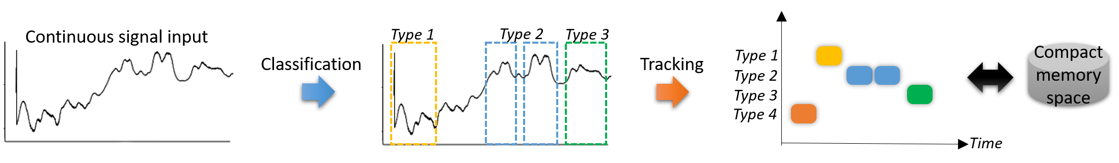
Figure 1. Basic framework of a system for timely classification and tracking of continuous signals, using compact local memory space.

Basic framework of a system for timely classification and tracking of continuous signals, using compact local memory space.

In summary, we study tracking and monitoring systems to support that following functions:

1. Timely learning and classifying patterns of continuous signals from known classes of signal patterns.

2. Timely learning and classifying unknown patterns of continuous signals.

3. Timely tracking occurrences of signal patterns of interests using small local memory space.

In particular, we focus on the application of smart plugs, which can provide a practical testbed for evaluating the tracking and monitoring system solutions. We developed standalone smart plugs that are capable of timely classification of appliance types and tracking of appliance behavior in a standalone manner. We built and implemented a smart plug prototype using low-cost Arduino platform with a small amount of memory space. Nonetheless, our system designs are also sufficiently generic for other timely monitoring and tracking applications of continuous signals.

The rest of the paper is organized as follows. Section 2 provides a review of the relevant background. We formulate the problems of timely pattern classification and occurrence tracking that are implemented in the smart plug system in Section 3. The techniques and algorithms of timely pattern classification and occurrence tracking are provided in Sections 4 and 5, respectively. We present a prototype implementation of a smart plug system in Section 6, and its detailed experimental evaluation study in Section 7. A survey of related work is provided in Section 8. Finally, we conclude the paper and discuss future extensions in Section 9. A table of key notations and their definitions is provided in Appendix.

2. Background

Efficient tracking of continuous signals over time is critical to several cyber-physical systems. In this work, we adopt streaming data algorithms for tracking the occurrences of signal patterns in embedded systems. There have been extensive theoretical studies of streaming data algorithms for counting problems (e.g., heavy hitters (Cormode et al., 2008), frequency moments (Zhao et al., 2005; Lall et al., 2006; Estan et al., 2006)). In the past, the applications of these studies are related to database systems and network traffic measurement. In this paper, we focus on the specific application to cyber-physical systems for tracking continuous signals. A novel contribution of this work is to implement streaming data algorithms for tracking the occurrences in embedded systems. The implementation of streaming data algorithms in embedded systems faces several new challenges, as these systems can only handle simple data processing, without sophisticated mathematical processing capability.

In this work, a smart plug prototype is developed for the classification of appliance types and behavior. Traditionally, the classification tasks for appliances can be achieved using either non-intrusive methods (Hart, 1992) or intrusive methods. Non-intrusive methods involve passive measurements of power consumption of the entire apartment and disaggregating the data to identify individual appliances, whereas intrusive methods require active measurements of power consumption of individual appliances using special power meters or smart plugs. Our smart plug prototype employs intrusive methods. Note that most of the prior studies of appliance classification were carried out by simulations using offline data collection. Few recent studies have implemented in embedded systems. For example, a system prototype is presented in (Ambati and Irwin, 2016), called AutoPlug, which can perform appliance classification and identification on a wireless gateway connecting to multiple power plugs. Unlike our smart plug prototype using resource-constrained Arduino platform, AutoPlug is based on more powerful Raspberry Pi 2 platform.

Overall, there are several differences between our study and the prior studies as follows.

1. Most of the proposed non-intrusive, as well as intrusive methods, do not perform near real-time appliance identification and instead deal with pre-recorded data in an offline manner. Our smart plug, on the other hand, is able to perform timely monitoring and classification of appliances using only the data seen thus far, without any knowledge of the future data.

2. Some recent efforts have also explored near real-time appliance identification. However, there are several fundamental differences with this work. For example, we focus on resource-constrained embedded system platform and online algorithms. See Section 8 for a detailed comparison.

3. Our smart plug is developed to support efficient streaming data algorithms, unlike other simple smart plug projects. It can perform advanced processing tasks locally in an online manner using small memory space, which requires very efficient implementation of the processing algorithms.

4. The existing classification and tracking algorithms are not designed for embedded systems in mind. Thus, we make non-trivial modifications to the existing algorithms so that it can be implemented in smart plug using limited processing power and memory size.

Furthermore, the contributions of this paper are summarized as follows.

1. We devised techniques and algorithms to perform timely classification of continuous signals (as opposed to the classification of discrete data in the extant literature). Our techniques are efficient to run on low-cost embedded systems.

2. We designed algorithms based on streaming data to perform timely occurrence tracking using compact memory space in low-cost embedded systems, which is novel in traditional streaming data literature.

3. We implemented a hardware prototype of a smart plug and implemented all of the proposed techniques on the smart plug to process power consumption signals in a timely manner. Our hardware prototype demonstrated practical effectiveness of the methods in real-world applications of smart plugs, which has been demonstrated in limited extent in the state of the art.

4. We conducted detailed evaluations of our techniques and prototype. Our evaluations show that our system can classify and track with good accuracy in compact memory space in real-world applications of smart plugs.

3. Problem Formulation

In this section, we formulate the problems of pattern classification and occurrence tracking that are implemented in the smart plug prototype. Note that a table of key notations and their definitions is provided in Appendix.

For generality, we first describe a generic setting of sensors that monitor and track certain continuous signals. We then apply to the specific setting of smart plugs.

3.1. Signal Classification

We denote by $x$ a stream of continuous signals observed by a sensor. For convenience, we assume slotted time, such as $(x_{1},x_{2},x_{3},...)$. The signals may be triggered by various events at different times that are not revealed to the sensor. Given the continuous nature of signals, the sensor needs to interpret and identify the states and transitions embodied by the signals.

To classify the signal patterns, we first detect a proper segmentation of continuous signals, which captures the passages and terminations of specific patterns. Note that patterns of signals do not necessarily occur at a fixed time interval. In this work, segmentation is based on the detection of state changes, where signals can exhibit different characteristics at different times. For example, the consumption of appliances may exhibit various state transitions, such as different operation cycles of a washing machine. Next, segments of signals will be classified according to the following two approaches.

3.1.1. Known Classes of Signal Patterns

The signals may be triggered by a finite number of possible classes of signal patterns. The list of possible classes of signal patterns may be known by the sensor in a-prior. For example, signals exhibiting certain common stochastic properties can be triggered by a common class of signal patterns. Regarding smart plugs, there are common stochastic models suitable for describing the power consumption patterns of appliances, which can be used as the prior known knowledge for classifying power consumption signals.

3.1.2. Unknown Signal Patterns

Alternatively, one can employ a clustering algorithm to classify the signal patterns in a way to minimize the discrepancy in each cluster. Let $x[t_{1}:t_{2}]$ be the segment of signal from time $t_{1}$ to $t_{2}$, and ${\cal S}$ be a non-overlapping segmentation of time, such that if $(t_{1},t_{2}),(t_{3},t_{4})\in{\cal S}$, then $x[t_{1}:t_{2}]$ and $x[t_{3}:t_{4}]$ are non-overlapping segments of $x$. We denote the set of clusters of patterns by ${\cal C}$. For each $i\in{\cal C}$, denote $c_{i}$ be a canonical signal that is selected to represent a cluster of patterns. Let ${\sf d}\big{(}x[t_{1}:t_{2}],c_{i}\big{)}$ be a distance metric between $x[t_{1}:t_{2}]$ and $c_{i}$. One example of distance metric is $\ell_{2}$ norm that measures the total absolute discrepancy over the designated interval.

We aim to find suitable ${\cal S}$ and ${\cal C}$, as to minimize an objective of the following general form:

(1) $$\min_{{\cal S},{\cal C}}\ \rho|{\cal C}|+\sum_{i\in{\cal C}}\sum_{(t_{1},t_{2})\in{\cal S}_{i}}{\sf d}\big{(}x[t_{1},t_{2}],c_{i}\big{)}$$

where $\rho$ is a weight parameter, and ${\cal S}_{i}$ is the set of segments belonging to the $i$-th cluster, defined as follows:

(2) $$\begin{array}[]{@{}l@{}}{\cal S}_{i}\triangleq\Big{\{}(t_{1},t_{2})\in{\cal S}\mid{\sf d}\big{(}x(t_{1},t_{2}),c_{i}\big{)}\leq{\sf d}\big{(}x(t_{1},t_{2}),c_{j}\big{)},\forall j\in{\cal C}\backslash\{i\}\Big{\}},\end{array}$$

In particular, we consider $k$-mean clustering, such that the number of clusters is at most $k$, where $|{\cal C}|\leq k$, namely, minimizing the following objective:

(3) $$\min_{{\cal S},{\cal C}:|{\cal C}|\leq k}\ \sum_{i\in{\cal C}}\sum_{(t_{1},t_{2})\in{\cal S}_{i}}{\sf d}\big{(}x(t_{1},t_{2}),c_{i}\big{)}.$$

An optimal solution to the above objective function will yield a segmentation of the input signal into a set of clusters where similar signal patterns are classified into the same cluster.

3.2. Occurrence Tracking

After classifying the signals, we can track the occurrences of each pattern over time. A detailed tracking history may require large memory space, in particular when the time epoch is long, or the number of possible patterns is large. Hence, we focus on the notion of approximate tracking.

In general, there is a stream of items with multiple occurrences. We want to record the items with the most prominent occurrences when observing the stream continuously. Note that we do not know the number of distinct items in advance, and we want to use memory space much less than the number of distinct items in the stream.

Suppose that the set of observed patterns are ${\cal C}$. Note that ${\cal C}$ may be a large set. The occurrences of each pattern will be recorded over a limited time horizon ${\cal T}$. Let $N_{i}^{\cal T}$ be the true total number of occurrences of pattern $i\in{\cal C}$ in the time horizon ${\cal T}$. Our objective is that given a memory size ${\sf c}$, one can identify the occurrences of the common patterns with high accuracy relative to the length of epoch $|{\cal T}|$. Note that the difficulty is the memory size ${\sf c}$ is a fixed constant that cannot grow at the same rate as $|{\cal C}|$.

In approximate tracking, we aim to obtain an estimated total number of occurrences $\widehat{N}_{i}^{\cal T}$ at the end of ${\cal T}$. We are interested in an assured bound of error probability for accuracy guarantee from true total number of occurrences, called ($\epsilon,\delta$)-accurate estimation, which satisfies:

(4) $${\mathbb{P}}\Big{(}|{\widehat{N}}_{i}^{\cal T}-N_{i}^{\cal T}|\geq\epsilon\cdot|{\cal T}|\Big{)}<\delta,$$

where $\epsilon$ and $\delta$ are the parameters for controlling the trade-off between accuracy and memory size.

For smart plugs, we will record the occurrences of power consumption patterns in multiple intervals of time, for example, the last hour, the last day, the last 2 days, the last week, etc. In practice, the occurrences will be recorded in a rolling window fashion. Due to the limited memory space, some occurrences in different intervals will be aggregated over time. For example, we will merge the data of the last seven days into one single aggregate record for the last week. Hence, approximate tracking is required to support the merging of data.

4. Classifying Continuous Signals

This section presents the basic ideas, techniques, and algorithms for learning and classifying the patterns associated with continuous signals in an online manner. Although the ideas can be applied to generic applications of continuous signal monitoring and tracking, we particularly consider the setting of continuous power consumption signals of electrical appliances.

4.1. Pattern Detection

The first step is the detection of the patterns embodied by the continuous signals. For power consumption signals, an appliance may transit through several operating states, in which the power consumption patterns usually vary from one state to the next. A state transition may be characterized by multiple components. The same state transition may also occur at several discrete levels of the input signals. We aim to identify such state transition patterns in the continuous signals. More specifically, we propose an online algorithm to detect state transition patterns by analyzing the continuous data stream.

4.1.1. Offline Detection

We first describe how patterns can be detected from the recorded data in an offline manner. This algorithm is proposed in (Iyengar et al., 2016). It is based on the concept of Approximate Entropy (ApEn) and Canny Edge Detection. ApEn is a metric for estimating the repeatability or predictability of a time series (Pincus, 1991). It was originally developed for heart rate analysis and later is applied to a wide range of applications such as psychology and financial analysis. ApEn of a time series $(x_{i})_{i=1}^{N}$ is computed in the following steps:

1. Fix two parameters: a positive integer $m$ and a positive real number $\theta$, where $m$ represents the length of a sub-sequence, and $\theta$ is the similarity threshold between a pair of sub-sequences.

2. Consider the set of sub-sequences of length $m$ in $x$, defined by $s^{m}=\big{\{}x[i:i+m-1]\big{\}}_{i=1}^{N-m+1}$.

3. For each $i$, define $C_{i}^{m}(\phi)$ as the fraction of sub-sequences in $s^{m}$ that are similar to $x[i:i+m-1]$. Two sub-sequences, $x[i:i+m-1]$ and $x[j:j+m-1]$, are similar if the difference between any pair of the corresponding values in the sub-sequences is less than or equal to $\theta$, namely,

   (5) $$|x_{i+k}-x_{j+k}|\leq\theta,\quad\mbox{for all\ }k\in\{1,...,m\}.$$

4. Finally, ${\tt ApEn}$ is computed as follows:

   (6) $${\tt ApEn}((x_{i})_{i=1}^{N})=\frac{1}{N-m+1}\sum_{i=1}^{N-m+1}\log C_{i}^{m}-\frac{1}{N-m}\sum_{i=1}^{N-m}\log C_{i}^{m+1}.$$

${\tt ApEn}$ can be used to measure the regularity in power consumption signals. Specifically, if similar power consumption patterns are similar, then ApEn will be small. Conversely, if there are irregular patterns, then ApEn will be large.

Input: $x,\ \phi,\ \omega$

1 forall $i\in\{1,...,|x|-\phi\}$ do

2    $H_{i}\leftarrow{\tt ApEn}(x[i:i+\phi])$

3 end forall

4$E^{\prime}\leftarrow{\tt CannyEdge1D}\big{(}(H_{i})_{i=1}^{|x|-\phi}\big{)}$

5 $E\leftarrow{\tt RemoveCloseEdges}(E^{\prime},\omega)$

return $E$

Algorithm 1 OFLStateTrans

Initialization : $E\leftarrow\varnothing$

Input: $x,\ t_{\rm now},\ \phi,\ \omega,\eta$

1 $H_{t_{\rm now}}\leftarrow{\tt ApEn}(x[t_{\rm now}-\phi:t_{\rm now}])$

2 $E^{\prime}\leftarrow{\tt CannyEdge1D}\big{(}(H_{i})_{i=t_{\rm now}-\eta}^{t_{\rm now}}\big{)}$

3 $E^{\prime\prime}\leftarrow{\tt RemoveCloseEdges}(E^{\prime},\omega)$

4 if $t_{\rm now}\in E^{\prime\prime}$ then

5    $E\leftarrow E\cup\{t_{\rm now}\}$

6 end if

Algorithm 2 ONLStateTrans

Algorithm 1 (OFLStateTrans) presents the offline state transition detection. First, it computes ApEn for every sub-sequence of length $\phi$. Then, it employs canny edge detection algorithm (Canny, 1986) on $(H_{i})_{i=1}^{|x|-\phi}$, which is an image processing technique for extracting boundaries from images. Since we consider one-dimensional data, OFLStateTrans uses a 1D variant of canny edge detection (${\tt CannyEdge1D}$) to analyze the list $(H_{i})_{i=1}^{|x|-\phi}$ and identify rapid changes in three steps:

1. Smooth the list $(H_{i})_{i=1}^{|x|-\phi}$ to remove noise by convolution with a digitalized Gaussian filter.

2. Take the first derivatives of the smoothed list to obtain the changes. In 1D setting, the peaks in the first derivatives represent potential edges.

3. Return the edges from the list of potential edges only with large magnitudes.

Finally, the edges that have less than $\omega$ in separation distance will also be removed. Fig. 2 illustrates the state transitions detected by Algorithm 1 (OFLStateTrans) on a sample trace of power consumption signals. OFLStateTrans can correctly detect many state transitions, by which segmentation of the continuous signals can be constructed.

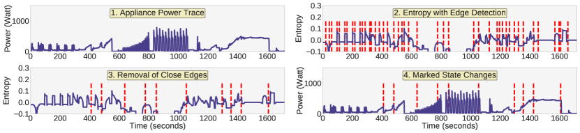
Figure 2. An illustration of the state transitions detected by Algorithm 1 (OFLStateTrans).

An illustration of the state transitions detected by Algorithm 1 (OFLStateTrans).

4.1.2. Online Detection

Algorithm 2 (ONLStateTrans) presents the online state transition detection using only the data observed thus far without complete knowledge of future data. It operates with a sliding window by computing ApEn for a window of $\eta$ timeslots. It will decide if an edge is detected at the current time $t_{\rm now}$ based on CannyEdge1D using the data of the last $\eta$ timeslots. The difference between the online and offline algorithms is that the online algorithm is based on myopic information of the last $\eta$ timeslots rather than the full information of every sub-sequences in the whole time horizon. We will evaluate the performance of ONLStateTrans in Section 7.

4.2. Classification with Known Classes of Patterns

Once a state transition is detected, we extract the corresponding segment of signals and classify it by a fitting an analytic model to the signals. There are a number of basic power consumption models suitable for describing the power consumption rates of appliances (Barker et al., 2013; Iyengar et al., 2016):

1. On-off Model: This model has a certain fixed power consumption rate $P_{\rm on}$ when active.

2. On-off Decay Model: The power consumption rate follows an exponential decay curve, dropping from the initial surge power $P_{\rm peak}$ to a stable power $P_{\rm active}$ at a decay rate $\lambda$.

   (7) $$P(t)=P_{\rm active}+(P_{\rm peak}-P_{\rm active})^{-\lambda t}$$

3. On-off Growth Model: The power consumption rate follows a logarithmic growth curve, starting with a level $P_{\rm base}$ and a growth rate $\lambda$ .

   (8) $$P(t)=P_{\rm base}+\lambda\cdot\ln t$$

4. Stable Min-Max Model: The power consumption rate is characterized by stable power $P_{\rm stable}$ with random upward or downward spikes $P_{\rm spike}$. The magnitude of random spikes is uniformly distributed between $P_{\rm stable}$ and $P_{\rm spike}$, and the inter-arrival times of spikes follow an exponential distribution with mean $\lambda$.

5. Random Range Model: The power consumption rate is similar to a random walk between a maximum power $P_{\rm max}$ and a minimum power $P_{\rm min}$.

6. Cyclic Model: The power consumption rate exhibits repetitive patterns.

Resistive and inductive appliances exhibit on-off, on-off decay, or on-off growth behavior, whereas appliances with non-linear power consumption (e.g., with non-sinusoidal current waveform) exhibit stable-min, stable-max, or random-walk behavior. In addition, many composite appliances (e.g., fridge, washing machine, air-conditioner) are composed of a combination of resistive, inductive and non-linear basic loads, which exhibit more complex power consumption patterns.

Given a segment of power consumption signals, the smart plug derives the model that best matches the observed power consumption rate. First, it differentiates the segment and compares its standard deviation with that of the original segment. If the standard deviation has decreased after differentiation, then the segment is best to be fit by a deterministic curve. On the other hand, if the standard deviation has increased, then the segment is best to be fit by a probability distribution. The details of model fitting are described as follows:

• For on-off and on-off growth models, it employs ordinarSection 7y linear least squares (OLS) method, which is a mathematical procedure for finding the best fitting curve to a given set of points by minimizing the sum of the squares of the residuals (i.e., the offsets of the points from the curve).

• For on-off decay model, it employs a special technique proposed in (Jacquelin, 2009). Fitting an exponential decay curve involves three parameters (i.e., $P_{\rm peak}$, $P_{\rm active}$, and $\lambda$). The best fit model is chosen as the one with the least discrepancy.

• For stable min, stable max and random range models, we follow the approach proposed in (Barker et al., 2013) in order to fit a probability distribution to the segment. Specifically, for stable min and stable max models, it derives $P_{\rm spike}$ as the mean of the data plus two standard deviations, and $\lambda$ as the average duration between spikes. To estimate $P_{\rm stable}$, it smooths the data by removing the spikes and estimates $P_{\rm stable}$ from the smoothed data using linear regression. In case of the random range model, the parameters $P_{\rm max}$ and $P_{\rm min}$ are obtained by simply choosing the maximum and minimum values in the data. As before, the best fit model is chosen as the one with the least discrepancy.

• For cyclic model, it uses autocorrelation to determine repeating patterns in the data as proposed in (Iyengar et al., 2016). If the data is cyclic, then its autocorrelation will attain a local maximum at each lag that is a multiple of the cycle period. It computes the autocorrelation of the data for up to $n$ lags and sees if the local maxima are separated by similar distances. If so, then the distance between the local maxima is determined as the duration between cycles.

4.3. Classification of Unknown Patterns

In the previous section, we assumed that a pattern always belongs to a finite number of classes (e.g., power consumption models), which may be known by the smart plug in advance. In this section, we allow these patterns to be unknown to the smart plug. In this paper, we focus on the approach of online learning of unknown patterns (GGMMc2008cluster). Alternatively, one can learn unknown patterns offline and then using it online. But this requires considerable a-prior training data, more memory and more latency for learning, which is not always desirable in IoT applications. On the other hand, we are able to demonstrate that learning and classifying of unknown patterns in an online manner can be achieved efficiently even using resource-constrained platforms.

For the case of unknown patterns, we employ online clustering algorithm (ONL$k$MeanCluster) to group the patterns detected by Algorithm 2 into clusters such that the patterns within a cluster are similar to each other but different from those in other clusters. Each cluster can be regarded as a canonical state of the appliance. We note that the segment length of continuous signals in one cluster may be different since the state transitions do not necessarily occur at fixed time intervals. Thus, we need an abstract representation of the patterns to facilitate consistent clustering. To this end, we use the following five attributes to represent each segment of continuous signal:

• Measures of central tendency: (i) arithmetic mean, (ii) median, and (iii) mode.

• Measures of statistical dispersion: (iv) standard deviation, and (v) range.

Next, all segments of continuous signals will be clustered based on a tuple of these five attributes.

ONL$k$MeanCluster is based on Doubling Algorithm (Charikar et al., 1997) and Online k-Means Clustering with Discounted Updating Rule (King, 2012), as described in Algorithm 3. While there are other clustering algorithms with advanced machine learning capabilities, k-means is often regarded as the simplest approach with efficient implementation and small memory requirement. also, the efficient implementation of K-means clustering algorithm can facilitate the implementations of more sophisticated clustering algorithm with advanced machine learning capabilities. The algorithm aims to find a suitable solution to the problem given in Eqn. (3). It consists of two stages: the update stage and the merging stage. In the update stage, the algorithm adds each segment either to an existing cluster or puts it in a new cluster. This stage continues for as long as the number of clusters is less than or equal to $k$. When the number of clusters exceed $k$, then the algorithm proceeds to the merging stage. In the merging stage, the algorithm reduces the number of clusters by merging clusters that are within a certain distance of each other. The merging stage guarantees that no more than $k$ clusters are selected in the presence of streaming data input. The detailed description of the clustering algorithm is given in Algorithm 3, as follows.

Input: Segment at time $t$: $z_{t}$, Max num. of clusters: $k$, Weight: $\alpha$

Initialization : ${\cal C}\leftarrow\big{\{}\{z_{i}\}_{i=1}^{k}\big{\}}$, ${\cal Z}\leftarrow\left\{z_{i}\right\}_{i=1}^{k}$, $d^{*}\leftarrow\underset{c_{1},c_{2}\in{\cal Z}:~{}c_{1}\neq c_{2}}{\min}\ \|c_{1},c_{2}\|^{2}_{2}$

1 if $|{\cal C}|\leq k$ then $\triangleright$ Updating clusters

2    $i\leftarrow\underset{i\in\{1,...,k\}}{\arg\min}\ \|z_{t},c_{i}\|^{2}_{2}$

3     $\triangleright$ Get the nearest cluster to $z_{t}$

4    if $\|z_{t},c_{i}\|^{2}_{2}\leq 2d^{*}$ then

5       ${\cal C}_{i}\leftarrow{\cal C}_{i}\cup\{z_{t}\}$

6        $\triangleright$ Add segment $z_{t}$ to the nearest cluster ${\cal C}_{i}$

7       $c_{i}\leftarrow c_{i}+\alpha(z_{t}-c_{i})$

8        $\triangleright$ Update the cluster center

9      

10   else

11       ${\cal C}\leftarrow{\cal C}\cup\big{\{}\{z_{t}\}\big{\}}$

12        $\triangleright$ Create a new cluster comprising of $z_{t}$

13      

14    end if

15   

16 end if

17if $|{\cal C}|>k$ then $\triangleright$ Merging clusters

18    $(i,j)\leftarrow\underset{i,j\in{\cal Z}\mid i\neq j}{\arg\min}\ \|c_{i},c_{j}\|^{2}_{2}$

19     $\triangleright$ Find two closest clusters

20    ${\cal C}^{\prime}\leftarrow{\cal C}_{i}\cup{\cal C}_{j}$

21     $\triangleright$ Merge two closest clusters

22    $c^{\prime}\leftarrow\frac{1}{|{\cal C}^{\prime}|}\underset{y\in C^{\prime}}{\sum}y$

23     $\triangleright$ Center of the merged cluster

24    ${\cal C}\leftarrow{\cal C}\cup\{{\cal C}^{\prime}\}\backslash\{{\cal C}_{i},{\cal C}_{j}\}$

25     $\triangleright$ Update clusters

26    ${\cal Z}\leftarrow{\cal Z}\cup\{c^{\prime}\}\backslash\{c_{i},c_{j}\}$

27     $\triangleright$ Update cluster centers

28    $d^{*}\leftarrow 2d^{*}$

29     $\triangleright$ Double the threshold of creating a new cluster

30   

31 end if

Algorithm 3 ONL$k$MeanCluster

• Initialization: The algorithm starts by initializing the first $k$ segments as the initial clusters, where ${\cal C}$ denotes the set of clusters and ${\cal Z}$ denotes the set of cluster centers. Initially, each segment itself is the cluster center since each cluster has only one segment. The minimum inter-cluster distance in ${\cal C}$ is denoted by $d^{*}$.

• Updating Clusters: Upon receiving a new segment $z_{t}$, the algorithm finds the cluster whose center is the nearest to $z_{t}$. If the distance between the nearest cluster center and $z_{t}$ is less than $2d^{*}$, then $z_{t}$ is added to the cluster and the cluster center is shifted proportionally. If, however, the distance is greater than $2d^{*}$, then a new cluster is created and segment $z_{t}$ is added to it. Notably, we use the discounted updating rule (i.e., $c_{i}\leftarrow c_{i}+\alpha(z_{t}-c_{i})$ ) instead of standard online k-Means updating rule (i.e., $c_{i}\leftarrow c_{i}+\frac{1}{|{\cal C}_{i}|}(z_{t}-c_{i})$) because the discounted update has been shown to provide a better result when the cluster centers are varying over time (King, 2012). The weight $\alpha\in(0,1)$ determines the relative weight of the new segment $z_{t}$, which provides an effect of exponential smoothing.

• Merging Clusters: Whenever the total number of cluster exceeds $k$, the merging step is invoked to reduce the total number of clusters within $k$. In this step, the algorithm first finds and merges the two closest clusters. Then, it adds the newly merged cluster to ${\cal C}$ and removes both old clusters from ${\cal C}$. Similarly, the center of the new cluster is added to ${\cal Z}$ and the old centers are removed. Finally, the cost of creating new clusters $d^{*}$ is doubled. The effect of doubling the cost is that, eventually, it will become prohibitively expensive to create new clusters. Thus, the algorithm will be more likely to assign new segments to one of the existing $k$ clusters.

We will evaluate the performance of ONL$k$MeanCluster in Section 7.

5. Memory-efficient Occurrence Tracking

In this section, we present the basic ideas, techniques, and algorithms for tracking of the pattern occurrences in the power consumption signals over time intervals of different lengths using the compact memory space of smart plug. In particular, we aim to keep track of the temporal occurrences for each pattern over the following intervals: (1) minute-by-minute occurrences of the past hour, (2) hourly occurrences of the past 24 hours, (3) daily occurrences of the past 30 days, (4) weekly occurrences of the past week, (5) monthly occurrences of the past year, and (6) yearly occurrences of the past year. Such detailed tracking will enable the smart plug to monitor the appliance behavior and usage patterns over a long period as well as identify the correlations in usage patterns.

However, the difficulty is that the memory space requirements for keeping individual track of every pattern for all of the above time intervals may exceed the small memory space of the smart plug. Thus, we focus on approximate tracking, by obtaining the estimated occurrences of the patterns using a special-purpose data structure called Count-min Sketch, which is a space-efficient probabilistic data structure that keeps an approximate count of elements in streaming data (Cormode and Muthukrishnan, 2005). Count-min sketch grows sub-linearly with the input data by randomly summarizing the data. At any given time, the sketch returns an estimated count of a certain pattern in response to a query. This estimated count is shown to be within a fixed threshold of the ground truth with a certain probability. Count-min sketch is similar to the Bloom Filter (Bloom, 1970). Bloom filter tells the membership of an element in the set, whereas count-min sketch tracks the approximate counts.

In essence, a count-min sketch employs $K$ hash functions to track the patterns (or items in general) using $M$ counters organized in a 2-dimensional ($K\times\frac{M}{K}$) array referred to as a sketch. The parameter $M$ specifies the memory space occupied by the sketch, whereas $K$ determines the time complexity of the sketch. These parameters are chosen during sketch creation in a way that not only makes them independent of the size of the stream but also bounds the discrepancy of the estimated count of a pattern from the ground truth. Recall that $N_{i}^{\cal T}$ is the true total number of occurrences of pattern $i\in{\cal C}$ in a certain epoch of time ${\cal T}$ and $\widehat{N}_{i}^{\cal T}$ is the estimated total number of occurrences. By setting $K=\ln\frac{1}{\delta}$ and $M=\ln\frac{1}{\delta}\cdot\frac{e}{\epsilon}$, we obtain ${\mathbb{P}}\big{(}|{\widehat{N}}_{i}^{\cal T}-N_{i}^{\cal T}|\geq\epsilon\cdot|{\cal T}|\big{)}<\delta$, where $\epsilon$ bounds the discrepancy between ${\widehat{N}}_{i}^{\cal T}$ and $N_{i}^{\cal T}$, while $\delta$ bounds the probability of discrepancy. This implies that the probability of discrepancy between the estimated count and the true count of pattern $z$ being more than $\epsilon T$ is at most $\delta$. A proof can be found in (Mitzenmacher and Upfal, 2017).

5.1. Hash Functions

To implement count-min sketch, we first need to implement hashing efficiently in the smart plug. Hashing can be regarded as a random projection from a high dimensional space of data to a low dimensional space of hashes. In the count-min sketch, each pattern is mapped by the $K$ independent hash functions, where the $i$-th hash function $h_{i}$ maps the pattern into one of the $\frac{M}{K}$ counters in the $i$-th row of the sketch. The hash functions are drawn independently at random from a 2-universal class of hash functions in the form of:

(9) $$h(x)=((ax+b)\ {\rm mod}\ p)\ {\rm mod}\ M.$$

The parameters are explained as follows.

• $x$ is a numeric representation of the pattern we will hash. Note that this requires a translation function to convert each pattern to a numeric form. To this end, we first calculate the string hash of a pattern using Secure Hash Algorithm 1 (SHA1) (Eastlake 3rd and Jones, 2001), then convert the string representation of the hash to a 32-bit number. We are constrained to using 32-bit numeric representation instead of 64-bit or 128-bit due to the hardware limitation of the smart plug. Similarly, SHA1 is chosen due to its ease of implementation in the smart plug.

• $p$ is a large prime number so that every possible key $x$ is in the range [0, $p-1$]. To satisfy this constraint, we set $p$ to be the smallest prime number greater than $2^{32}-1$ since any 32-bit positive number must be in the range [0, $2^{32}-1$].

• $a$ and $b$ are any numbers in the range [1, $p-1$] and [0, $p-1$], respectively.

Every possible combination of $a$ and $b$ in Eqn. (9) results in a different hash function. The total number of possible hash functions is $p(p-1)$ since we have $p$ choices for $b$ and $p-1$ choices for $a$. We can easily generate the $K$ hash functions for count-min sketch, simply by substituting $K$ different combinations of $a$ and $b$ in Eqn. (9). Notably, any hash function drawn from 2-universal family has a property that the probability of two different keys $x_{i}$ and $x_{j}$ being mapped into the same counter is $\frac{1}{M}$, where $M$ is total number of counters. In count-min sketch, however, each hash function ranges over a row of the counters instead of all $M$ counters, thus the collision probability is given by (Mitzenmacher and Upfal, 2017):

(10) $$\mathbb{P}\{h(x_{i})=h(x_{j})\}=\frac{K}{M}.$$

5.2. Updates on Counters

There are multiple ways to optimize the performance of count-min sketch. One possible way is to choose proper updating rules on the counters upon each occurrence. For every occurrence $t$ of the $i$-th pattern in the streaming data, we apply each of the $K$ hash functions to obtain $C_{i,h_{t}^{i}}$ (the $h_{t}^{i}$-th counter in the $i$-th row of the sketch).

1. First, we can update the counter using the following rule:

   (11) $$\text{\bf(Update Rule {\tt U1})}\qquad C_{i,h_{t}^{i}}\leftarrow C_{i,h_{t}^{i}}+1.$$

2. Alternatively, we can perform a more conservative update by using the following rule:

   (12) $$\text{\bf(Update Rule {\tt U2})}\qquad C_{i,h_{t}^{i}}\leftarrow\max\Big{\{}C_{i,h_{t}^{i}},\underset{j\in\{1,...,K\}}{\min}\{C_{j,h_{t}^{j}}\}+1\Big{\}}.$$

The modification in Eqn. (12) can achieve improved error performance in practice. We note that each update operation requires computing only a small number of hash functions and basic arithmetic, which has fast running time.

5.3. Retrieval from Counters

Since the count-min sketch randomly summarizes the data in the counters. A proper retrieval rule from the counters will affect the accuracy of approximate tracking.

1. First, we can retrieve the values of counters of the $i$-th pattern by taking the minimum of all the counters mapped by the corresponding hash functions:

   (13) $$\text{\bf(Retrieval Rule {\tt R1})}\qquad N_{i}=\underset{i\in\{1,...,K\}}{\min}\{C_{i,h_{t}^{i}}\}.$$

   Note that $N_{i}$ is an overestimate of the true count of occurrences (i.e., $N_{i}\geq T_{i}$), because multiple items can be mapped to the same counter by a hash function.

2. On the other hand, to tackle the problem of overestimation, the following alternative rule to Eqn. (13) is proposed in (Goyal et al., 2012):

   (14) $$\text{\bf(Retrieval Rule {\tt R2})}\qquad N_{i}=\underset{i\in\{1,...,K\}}{\rm median}\left\{C_{i,h_{t}^{i}}-\frac{\sum_{j=1}^{K}[C_{i,j}-C_{i,h_{t}^{i}}]}{\frac{M}{K}-1}\right\}.$$

   Eqn. (14) basically deducts the estimated noise $(\frac{\sum_{j=1}^{K}[C_{i,j}-C_{i,h_{t}^{i}}]}{\frac{M}{K}-1})$ from each of the $K$ counters and returns the median of the resulting $K$ values as the estimated count $N_{i}$.

An integrated approach is also possible – taking the minimum of Eqns. (13) and (14) as the estimated count $N_{i}$, because Eqn. (14) might actually overestimate $N_{i}$ more than Eqn. (13).

In the experimental evaluation study in Section 7, we will evaluate the effectiveness of the update and retrieval rules on practical power consumption data traces in the smart plug.

6. Prototype Implementation

In this section, we present the hardware prototype implementation for the smart plug. Our smart plug prototype enables extensive testing and evaluations in real-world scenarios with home appliances.

6.1. Hardware Platform

The smart plug requires appropriate embedded systems for the timely computation of the classification and tracking tasks. With this in mind, we developed the smart plug prototype based on Arduino-compatible WiFi-enabled ESP-12s hardware platform (Systems, 2017). Unlike other Arduino-family micro-controller boards (e.g., Arduino Uno, Nano, Micro, and Pro), ESP-12s has enough processing power and memory size to compute the required tasks for timely processing. Table 1 summarizes and compares the specifications of ESP-12s with the Arduino-family boards of similar physical footprint.

Table 1. ESP-12s versus the Arduino-family boards.

Type	Clock Speed	Static RAM	Flash Memory	WiFi	Cost (as in Jun, 2017)
ESP-12s	80 MHz	82 kB	1 MB	yes	$\leq$ $4.0
Arduino Pro/Nano	16 MHz	2 kB	32 kB	no	$\leq$ $3.5
Arduino Micro	16 MHz	2.5kB	32 kB	no	$\leq$ $9.0

The list of parts/components used in the smart plug prototype is provided in Table 2. In our prototype, we have managed to keep the total cost as low as $20 per device.

Component	Quantity	Cost (as in June 2017)
ESP-12S Arduino micro-controller (Wemos D1 Mini)	1	$\leq$ $4.0
Relay (Wemos DC 5V relay shield)	1	$\leq$ $2.0
Current sensor (ACS712-20A)	1	$\leq$ $2.0
Analog multiplexer (74HC4052 or 74HC4051)	1	$\leq$ $2.0
Circuit-mount 220V-5V power supply	1	$\leq$ $3.5
Capacitors (10 $\mu$F, 440 nF)	2	$\leq$ $2.0
Resistors (100 k$\Omega$, 10 k$\Omega$, 5.1 k$\Omega$)	5
Universal size perforated PCB (5 x 7 cm)	1	$\leq$ $3.0
Push button for WiFi	1
Power jack for 2.1mm for transformer	1
Total Cost		$\leq$ $20

Table 2. List of parts/components used in the smart plug prototype .

6.2. Smart Plug Prototype

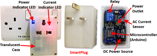
Figure 3. Hardware prototype of the smart plug.

Hardware prototype of the smart plug.

Fig. 3 shows the hardware prototype of the smart plug. The smart plug contains a relay to control the power supply to the connected appliance, and several sensors to measure the instantaneous AC voltage and current of the appliance. The AC current is measured using Hall effect-based linear current sensor (ACS712). The AC voltage can be measured using an external 220V–9V step-down voltage transformer. The smart plug can perform the following functions:

1. Appliance Monitoring: The smart plug can perform sophisticated monitoring of the power consumption behavior such as detection, classification, clustering, and tracking of the appliance as described in this paper. These monitoring tasks can enable further advanced functions (e.g., automated demand response, indirect monitoring of the occupant activities, and energy analytics).

2. Power Signature Identification: The ability to measure instantaneous voltage and current enables the computation of a variety of quantities regarding the power consumption, such as active power, reactive power, apparent power, root-mean-square voltage, root-mean-square current, and power factor. The knowledge of these power consumption quantities can give an accurate identification of power consumption signals for appliances, which will be useful for appliance identification, diagnosis, and fault detection.

3. Remote Control: The smart plug supports remote control of the appliance by a WiFi connection. It provides RESTful APIs for controlling the attached appliance and querying its status. The APIs can be accessed by basic HTTP commands from smartphones and web clients. An Internet-connected base station based on Raspberry Pi supports WiFi connections to multiple smart plugs. The smart plugs can transmit the power consumption data and its monitoring results to a third-party base station. The base station provides APIs that can be accessed by smartphones and web clients to visualize the data received from the smart plugs. The base station can provide remote access to the smart plugs for monitoring and control of appliances over the Internet.

6.3. System Architecture

To develop the smart plug prototype, we created a Fritzing (Software, 2017) diagram of the breadboard circuit. A Fritzing diagram contains the necessary detail for producing physical circuit boards. It also automatically generates printed circuit boards (PCB) from the circuit design. We created

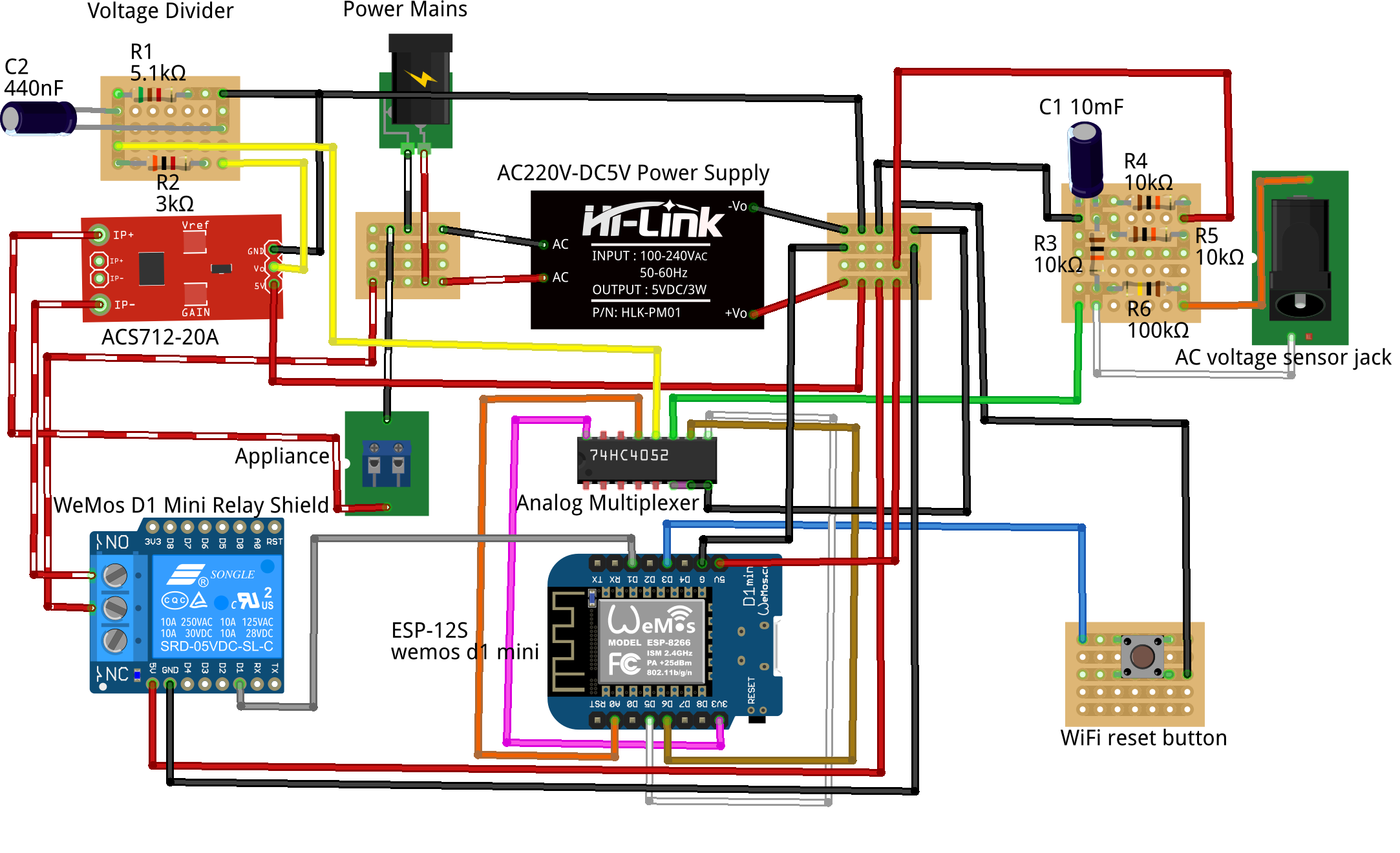
Figure 4. Fritzing diagram of the smart plug prototype.

Fritzing diagram of the smart plug prototype.

Fig. 4 depicts the Fritzing diagram for our smart plug prototype, with connectivity to all the components. In particular, the banded red wiring indicates 220V AC power connection, and the banded black wiring is the corresponding neutral connection. Notably, the AC voltage sensor circuit in the upper right corner of Fig. 4 is based on the circuit design in (to build an Arduino energy monitor measuring mains voltage and current, 2017). An external 220-9V AC-to-AC voltage transformer can be plugged into the AC voltage sensor jack, which will provide instantaneous AC voltage. If the voltage transformer is not connected, then the smart plug uses a fixed RMS voltage to calculate appliance power consumption. The voltage divider in the upper left corner of Fig. 4 is used to level shift the voltage output of the AC current sensor from 5V to 3V. The level shifting is necessary because the analog pin of ESP-12S has an operating voltage range of 0-3.2V. The analog multiplexer in the center of Fig. 4 is also needed because both the AC current sensor and AC voltage transformer provide analog signals, but ESP-12S micro-controller has only one analog input pin. Thus, the multiplexer enables ESP-12S to read both analog inputs. To minimize the form factor of the smart plug, we divided the overall circuit into several layers such that they can be stacked on top of each other.

6.4. Software System

The smart plug is required to carry out timely computation of various tasks involved in event detection, classification, and clustering (e.g., approximate entropy computation, edge detection, smoothing, linear regression, least square fitting, autocorrelation computation, k-means clustering, and hashing, etc.). To implement these tasks, we developed native modules in Arudino (C++) using object-oriented programming paradigm.

In addition, we also developed a web server along with a client graphical user interface (GUI) that allows for wireless interaction with the smart plug. The server provides RESTful API that can be used to query the power state of the smart plug and request data. The server is also implemented in Arduino (C++) and runs directly on the smart plug. The client GUI can be accessed from a web browser by navigating to the IP address of the smart plug. The smart plug supports two WiFi modes: (i) stand-alone access point (AP) mode, which allows users to directly connect to the smart plug without the need for a WiFi router, (ii) station mode, where the smart plug can connect to an existing WiFi router to become part of the local WiFi network.

Section 7.5 provides details regarding the size of the code and the memory requirements of our software system. Moreover, the source code of the smart plug software system is currently released publicly (sma, 2019) to give other researchers access to all aspects of the implementation and enable them to take advantage of our work for their future projects.

7. Experimental Evaluation

In this section, we provide a detailed experimental evaluation study of the techniques and algorithms proposed in this paper and implemented in the smart plug prototype.

7.1. Pattern Detection

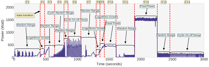
(a) Offline state transition detection using Algorithm 1 (OFLStateTrans).

Offline state transition detection using Algorithm 1 (OFLStateTrans).

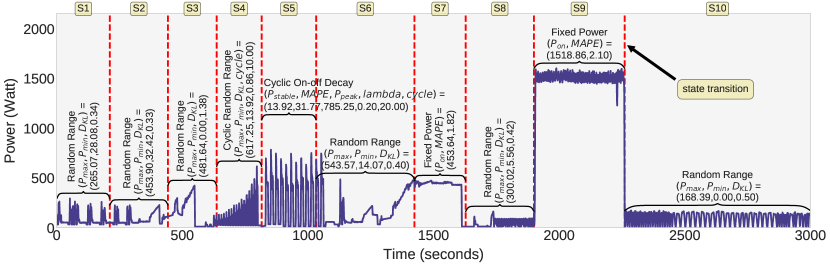
(b) Online state transition detection using Algorithm 2 (ONLStateTrans).

Figure 5. Results of state transition detection for the power consumption signals of a washing machine.

In this section, we discuss the performance evaluations of both offline and online algorithms. The results of state transition detection for a sample trace of power consumption of a washing machine are illustrated in Fig. 5. The washing machine is a composite load with several active power states, each corresponding to a constituent basic load. Each vertical dashed line in Fig. 5 indicates a state transition event. In particular, Fig. 5(a) shows the results by Algorithm 1 (OFLStateTrans), which can be compared with the results of Algorithm 2 (ONLStateTrans) in Fig. 5(b). The parameter values used by the algorithms during the experiment are listed in Table 3. The table shows that both algorithms use sliding window (of length $\phi$) in order to compute ApEn. However, Algorithm 1 operates over a sliding lookahead window assuming all future data is available, whereas Algorithm 2 operates over a sliding lookback window of a limited period of data. We observe that both algorithms are able to partition the sample trace into segments of states, as indicated by the vertical dashed lines in Figure 5. However, there are some differences between the results of the two algorithms in terms of the number of detected states and the respective times. In particular, OFLStateTrans has detected 14 states (S’1–S’14), while ONLStateTrans has returned only 10 states (S1–S10). The reason of this discrepancy is the unavailability of future data, which makes it hard for online algorithm to detect transitions between similar states.

	Edge	Sliding	Sub-sequence	Similarity	Online
	Separation	Window	Length	Threshold	Window
	Threshold ($\omega$)	Length ($\phi$)	($m$)	($\theta$)	Size ($\eta$)
Algorithm 1	60	60	$\phi/4$	$0.2\cdot\sigma(x[1:N])$	-
Algorithm 2	200	60	$\phi/4$	$0.2\cdot\sigma(x[t_{\rm now}-\phi:t_{\rm now}])$	7

Table 3. Values of parameters in the algorithms. $\sigma(\cdot)$ is the standard deviation of a time series.

We also evaluated the results of state transition detection for a sample trace with multiple appliances in Fig. 6. The trace is comprised of the power data from multiple appliances (i.e., lamp, microwave oven, laptop computer, LCD monitor, and iron), where at any given time only one appliance is connected to the smart plug. We intend to show that our system can automatically classify and track the consumption patterns, even when different appliances are plugged in at different times. Note that our smart plug is not trying to disaggregate the power data with multiple appliances at the same time. It can be observed in Fig. 6 that both the microwave oven and the iron have a high power consumption rate of more than 1000 Watts, whereas the laptop computer and the LCD monitor consume less than 100 Watts. Due to this large difference between their power consumption levels, it is difficult to depict the precise power consumption variations of laptop computer and LCD monitor from Fig. 6. Thus, portions of the sample trace corresponding to the laptop computer and the LCD monitor are zoomed in and shown using small plots inside Fig. 6. Again, ONLStateTrans is able to partition the sample trace into segments corresponding to the appliances through detection of state transitions from one appliance to another.

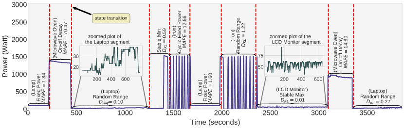
Figure 6. Results of online state transition detection using Algorithm 2 (ONLStateTrans) for the power consumption signals with multiple appliances.

Results of online state transition detection using Algorithm 2 (ONLStateTrans) for the power consumption signals with multiple appliances.

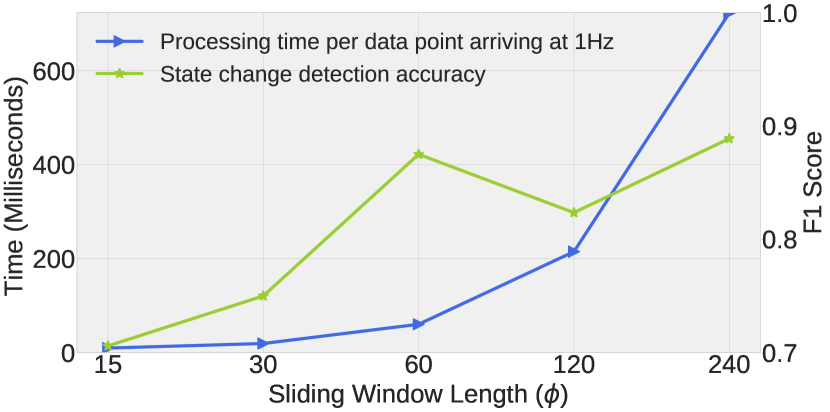
(a) Effect of the sliding window length.

Effect of the sliding window length.

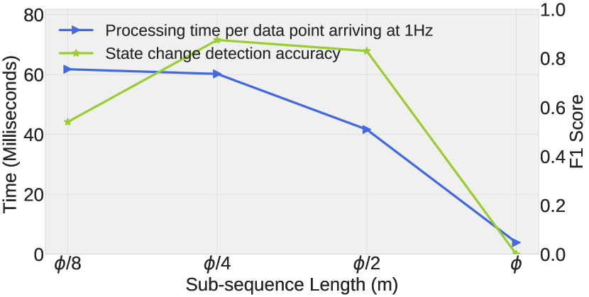
(b) Effect of the sub-sequence length.

Effect of the sub-sequence length.

Figure 7. Trade-off between performance and scalability of Algorithm 2 (ONLStateTrans).

The trade-off between performance and scalability is important for resource-constrained IoT devices like our smart plug. Therefore, we evaluated the smart plug with different values of the parameters listed in Table 3 to demonstrate this trade-off. In particular, we run the experiment with sliding windows and sub-sequences of different lengths and present the results in Fig. 7. The primary y-axis represents the processing time per data point arriving at 1 Hz (every second) and secondary y-axis show the performance of the algorithm in terms of F1 score. In Fig. 7(a), we can see that as we increase $\phi$, the performance is improved but the time complexity also increases. However, the performance gain beyond $\phi$=60 is negligible while the increase in time complexity is more than linear. Therefore, we use $\phi$=60 in our smart plug platform. Similarly, in Fig. 7(b), we can see that the algorithm achieves the best performance (highest F1 score) when m=$\frac{\phi}{4}$. The F1 score worsens when m=$\frac{\phi}{2}$ and drops to 0 when m=$\phi$. The proper values for the remaining parameters in Table 3 were calculated in a similar fashion.

7.2. Classification with Known Classes of Patterns

The results for classification according to known classes of patterns are depicted in Fig. 5. In particular, Fig. 5(a) depicts the learned models for segments, whereas Fig. 5(b) depicts the learned models along with the inferred parameters.

First, we discuss the performance of deterministic curve fitting. Originally, (Iyengar et al., 2016) proposes to employ non-linear least square method for curve fitting. Here, we instead employ linear least square method because non-linear least square method involves iterative optimization and requires more memory space that can be provided in the smart plug. Generally, both approaches are able to identify the best fit models of power consumption rates with reasonable accuracy. Furthermore, we observe that the classification outcomes of both approaches are comparable. For instance, the same model has been detected by both approaches for the following pairs of segments in in Figs. 5(a) and 5(b): (i) $(S^{\prime}3,S3)$, (ii) $(S^{\prime}6,S5)$, and (iii) $(S^{\prime}12,S9)$. In Fig. 6, we observe that with the exception of iron, our approach can identify the same model if it sees such an appliance again.

We evaluate the discrepancy of deterministic curve fitting by Mean Absolute Percentage Error (MAPE), defined as follows:

(15) $${\tt MAPE}=\frac{100}{N}\sum_{t=1}^{N}\frac{P_{t}-\hat{P_{t}}}{P_{t}}$$

where $P_{t}$ is the actual power consumption at time $t$, $\hat{P_{t}}$ is the predicted power consumption at time $t$, and $N$ is the total number of data points in the segment. A lower value of MAPE indicates better accuracy. We provide the values of MAPE in Fig. 5(b) and Fig. 6 in the respective segments (i.e., segments with curve fitting), which have reasonably low MAPE values in all cases except microwave oven, because the particular segment contains slightly imprecise detection of the state transition by ONLStateTrans.

Next, we evaluate the discrepancy of probability distribution fitting by Kullback-Leibler (KL) Divergence (Cover and Thomas, 2012), defined as follows:

(16) $$D_{\rm KL}(Y||X)=\sum_{i=1}^{N}Y(i)\log\left(\frac{Y(i)}{X(i)}\right)$$

where $Y$ is the true probability distribution of the segment and $X$ is the learned probability distribution. KL divergence indicates the information loss incurred by fitting a specific probability distribution to the data. We provide the values of KL divergence in Fig. 5(b) and Fig. 6 in the respective segments (i.e., segments with distribution fitting). A lower value of KL divergence indicates better accuracy. Based on the $D_{\rm KL}$ values in Fig. 5(b) and Fig. 6, we observe that the learned probability distribution is a good approximation to the true probability distribution in each segment.

7.3. Classification of Unknown Patterns

Fig. 8 depicts the results of Algorithm 3 (ONL$k$MeanCluster) when applied to cluster the segments in Fig. 5. There are 6 sub-figures in total, each representing a cluster. The plotted curves in the sub-figures represent segments of power consumption signals that are clustered together by ONL$k$MeanCluster. It can be observed that similar segments are indeed clustered together by ONL$k$MeanCluster. For instance, all three segments in Fig. 8d behave like a random range model. Likewise, the segments in Fig. 8b and Fig. 8f have cyclic patterns.

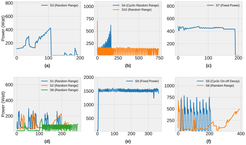
Figure 8. Results of classification of unknown patterns using Algorithm 3 (ONL$k$MeanCluster). Each sub-figure represents a cluster. X-axis indicates time in seconds for the signals. The legends indicate the segment ID along with their learned models in Fig. 5(b).

Results of classification of unknown patterns using Algorithm 3 (ONL$k$MeanCluster). Each sub-figure represents a cluster. X-axis indicates time in seconds for the signals. The legends indicate the segment ID along with their learned models in Fig. 5(b).

To evaluate the results of clustering, we use Sum of Squared Error (SSE), which is a standard metric used to measure the goodness of clustering without reference to external information. In particular, we use Within-cluster Sum of Squares Error (WSSE) and Between-clusters Sum of Squares Error (BSSE), computed by the following equations:

(17) $${\tt WSSE}=\sum_{i}^{k}\sum_{z\in{\cal C}_{i}}(z-c_{i})^{2},\qquad{\tt BSSE}=\sum_{i}^{k}|{\cal C}_{i}|(c-c_{i})^{2}$$

where $z$ is a pattern, ${\cal C}_{i}$ is the $i$-th cluster, $c_{i}$ is the center of the $i$-th cluster, $|{\cal C}_{i}|$ is the size of cluster $i$, and $c$ is the center of all clusters. WSSE measures how closely related are the patterns in a cluster (i.e., cohesion), while BSSE measures how well-separated the clusters are from each other (i.e., separation). A good value for $k$ is the one that minimizes ${\tt CH}=\frac{{\tt BSSE}/(k-1)}{{\tt WSSE}/(n-k)}$, where $n$ is total number of patterns, and CH is Calinski-Harabasz Index (Caliński and Harabasz, 1974). Table 4 lists the WSSE, BSSE, and CH for different values of $k$ when clustering the segments in Fig. 5 using ONL$k$MeanCluster.

Num. of clusters ($k$)	2	3	4	5	6	7	8
Output clusters	(S1,…,S8,S10);	(S5,S7,S10);	(S9); (S7);	(S1,S2); (S3);	(S3); (S7); (S9);	(S3); (S1,S2,S8);	(S6,S10); (S5);
	(S9)	(S1,S2,S3,S4,S8);	(S1,S2,S3,S8);	(S7); (S9);	(S1,S2,S8);	(S4,S10); (S5);	(S4); (S3); (S7);
		(S9)	(S4,S5,S6,S10)	(S4,S5,S6,S10)	(S4,S10); (S5,S6);	(S6); (S7); (S9)	(S8); (S9); (S1,S2)
Cohesion (WSSE)	16991017	18201188	19411360	20621532	21831704	23041875	24252047
Separation (BSSE)	49237745	66216277	83194810	100173343	117151876	134130409	151108941
Calinski-Harabasz Index (CH)	23.1	12.7	8.5	6.0	4.2	2.9	1.7

Table 4. Performance evaluation of Algorithm 3 (ONL$k$MeanCluster).

The second row in the table lists the resulting clustering of the segments for the given value of $k$, where each tuple represents a separate cluster. The last row shows that the clustering performance is improved as $k$ increases, but this also increases the number of clusters and the memory space.

Our results show that the results of clustering are acceptable when $k$=6 because similar segments are clustered together. Also, as discussed in Section 4.2, there are six basic power consumption models that describe the power consumption rates of most appliances. Therefore, choosing $k$=6 will ideally result in a separate cluster for each model and is, therefore, a logical choice.

A general problem with the online clustering algorithms is that the clustering quality may decrease when data streams evolve over time, causing the cluster centers to also shift over time. To address this problem, Algorithm 3, uses the discounted update rule which has been shown to yield comparatively better results when the cluster centers are evolving over time (King, 2012). In particular, we choose $\alpha$=1.0 in the discounted update rule, which creates the effect of exponential smoothing such that Algorithm 3 forgets the initial cluster centers over time and performs close to the optimal solution. Another typical problem with the standard $k$-means is that it may not be a good choice of the algorithm if the number of clusters is not known a priori. However, in the case of Algorithm 3, we already know the number of clusters in advance (i.e., $k$=6).

Figure 9 compares the performance of Algorithm 3 against the standard online $k$-means. As explained in Section 4.3, Algorithm 3 uses the discounted updating rule (i.e., $c_{i}\leftarrow c_{i}+\alpha(z_{t}-c_{i})$ ) instead of the standard online $k$-means updating rule (i.e., $c_{i}\leftarrow c_{i}+\frac{1}{|{\cal C}_{i}|}(z_{t}-c_{i})$). It can be seen that Algorithm 3 outperforms standard online $k$-means for all values of $k$.

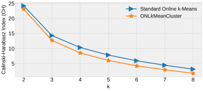
Figure 9. Comparison between ONL$k$MeanCluster and standard $k$-means.

Comparison between ONL$k$MeanCluster and standard $k$-means.

7.4. Occurrence Tracking

In this section, we present the evaluation results of occurrence tracking in the smart plug prototype. We tested various combinations of the update and retrieval rules from Sections 5.2 and  5.3. More specifically, we obtain evaluation results for occurrence tracking using the count-min sketch for the following combinations of update and retrieval rules:

1. Count-min (CM): Count-min sketch with regular update rule (Eqn. (11)) and regular retrieval rule (Eqn. (13)).

2. Count-min with conservative update (CM-CU): Count-min sketch with conservative update rule (Eqn. (12) and regular retrieval rule (Eqn. (13)).

3. Count-mean-min (CMM): Count-min sketch with regular update rule (Eqn. (11)) and a retrieval rule which takes the minimum of Eqns. (13) and  (14).

4. Count-mean-min with conservative update (CMM-CU): Count-min sketch with conservative update (Eqn. (12)) and the same retrieval rule as CMM.

Table 5 summarizes the above settings, indicating the update and retrieval rules along with the strength and weakness for each sketch. For example, CMM-CU uses update rule (Eqn. (12)), which reduces the overestimation during the update operations compared to update rule (Eqn. (11)).

Setting	Update Rule	Retrieval Rule	Strength	Weakness
CM	U1	R1	Simplicity	Overestimation
CM-CU	U2	R1	Reduced overestimation	More computation
CMM	U1	min{R1,R2}	Reduced noise	More computation
CMM-CU	U2	min{R1,R2}	Reduced noise, reduced overestimation	More computation

Table 5. Settings of different count-min sketches used in our tests.

For each setting, an evaluation study is conducted where the arrival patterns are first tracked by the minute-by-minute sketch. Then, the minute-by-minute patterns are aggregated into an hourly sketch. Next, the hourly patterns are aggregated into a daily sketch. The monthly and yearly sketches are computed in a similar manner. This way, we use different sketches (and therefore counters) to store occurrences at each level. At every level of the occurrence tracking (e.g., daily, monthly), the previous level sketch is reset after aggregation of its occurrence counts. For example, the counters in the hourly sketch are reset to zero after the daily occurrences are counted and stored in a daily sketch. The patterns are generated by our pattern detection and classification algorithms from synthetic streaming data of power consumption signal from a single appliance, comprising of more than one year’s data. To compare the errors between the estimated and the actual counts, we compute the exact counts of the patterns in every sketch (i.e., hourly, daily, and monthly). After processing all patterns in the streaming data, we query the sketches to generate approximate occurrence counts of the patterns. We set $M=500$ and $K=5$ during the experiments. Increasing $M$ and $K$ will improve tracking accuracy by reducing over-estimation. However, the smart plug has limited memory capacity, which means we cannot increase the parameter values indefinitely.

To measure the accuracy of the sketches, we use Mean Absolute Error (MAE) and Mean Relative Error (MRE). MAE is defined as the average of the absolute differences between the estimated and the actual counts of the patterns in a sketch, whereas MRE is obtained by dividing MAE by the total number of true occurrences of all patterns in the sketch:

(18) $${\tt MAE}=\frac{\sum_{i=1}^{n}|N(i)-T(i)|}{n},\qquad{\tt MRE}=\frac{\sum_{i=1}^{n}|N(i)-T(i)|}{nT}$$

MAE and MRE provide different insights. MAE measures the average magnitude of the errors and provides an indication of how big of an error we can expect from the count-min sketch on average. MRE, on the other hand, indicates how good the tracking performance of a sketch is relative to the number of the total patterns being tracked by the sketch. Note that the MRE of one sketch might be considerably smaller than that of another sketch, even though both sketches might have the same value of MAE.

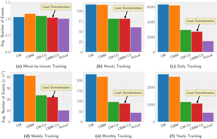
Figure 10. Results of occurrence tracking using count-min sketch.

Results of occurrence tracking using count-min sketch.

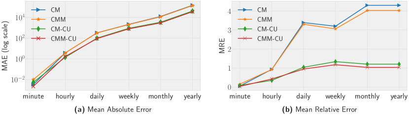
Figure 11. Occurrence tracking error using count-min sketch.

Occurrence tracking error using count-min sketch.

Fig. 10 depicts the occurrence tracking results. In particular, Figs. 10a-10c highlight the tracking performance for pattern counts over short intervals (i.e., minute, hour, day), whereas Figs. 10d-10f depict the tracking results for pattern counts over longer intervals (i.e., week, month, year). Each sub-figure provides a comparison between the actual count and estimated counts obtained by each count-min sketch as indicated by the X-tick labels. For instance, the bars in Fig. 10b compare the hourly occurrences (averaged over all patterns) between different sketches and the actual count. We obtain several observations:

1. Approximate tracking of patterns using count-mean-min with conservative update (CMM-CU) results in the least overestimation for all intervals from minute-by-minute to yearly tracking (Fig. 10a-10f). This suggests that conservative updating of the sketch and removing the estimated noise during retrieval operations significantly can improve the accuracy.

2. Fig. 11 compares the change in MAE and MRE by different sketches as the interval increases from a minute to full year. As guaranteed by count-min sketch (Cormode and Muthukrishnan, 2005), the error is due to overestimation and there is no under-estimation error by any sketch. In Fig. 11a, we observe that MAE has a linear growth rate on a logarithmic scale, which means it actually grows exponentially with the interval length. The exponential growth is exhibited by all the sketches in Fig. 11a. On the other hand, MRE provides a different picture from MAE as shown in Fig. 11b. It shows that CM-CU and CMM-CU achieve superior accuracy compared to the remaining two sketches, with CMM-CU as the best among all sketches which can be verified from Fig. 10.

3. We observe that MAE mounts as the interval length increases. This is because when we aggregate data from one sketch to another, the error is also aggregated. For instance, the hourly estimates returned by the sketch for a pattern already contain overestimation errors. When we add them together to get the pattern’s daily estimate, we implicitly add these individual hourly overestimation errors. Similarly, the weekly estimate of a pattern contains errors from both the hourly and daily estimates, and so on.

4. Intuitively, increasing $M$ and $K$ reduces the overestimation error as already shown in (Deng and Rafiei, 2007) and (Shi et al., 2011). In our cases, however, the values of $M$ and $K$ are dictated by the memory and processing capabilities of the smart plug prototype.

From these observations, the setting CMM-CU is shown to be desirable for tracking in the smart plug.

7.5. Computational and Energy Overheads

A key performance metric of the smart plug prototype is the computational overheads. Table 6 lists the computational overhead for various tasks performed by the smart plug prototype. For each task, the table provides the running time required by the smart plug prototype to execute the task in increasing order of complexity. In the case of classification of known classes of patterns, for instance, the running time of the smart plug grows sub-linearly with the data length. For the remaining two tasks (i.e., autocorrelation and approximate entropy), the growth is slightly more than linear. Notably, the last column represents the maximum complexity of the given task. Overall, the smart plug prototype still performs most tasks efficiently in a timely manner. We note that the first three tasks listed in the table are related to pattern detection and classification. We have also included the computational overhead calculations for occurrence tracking. We note that each update operation requires computing only a small number of hash functions and basic arithmetic, which takes very small processing time.

Autocorrelation	Lag ($k$)	50	100	200	400
	Running Time (milliseconds)	24	88	344	1351
Classification	Data Length ($N$)	200	400	800	1600
	Running Time (milliseconds)	529	711	1085	1564
Approximate Entropy	Sliding Window Length ($\phi$)	60	120	240	480
	Running Time (milliseconds)	60	214	722	2310
Count-min Sketch Updates	Number of counters in sketch ($M$)	100	200	400	600
	Running Time (milliseconds)	7	9	10	13

Table 6. Computational overheads of processing in the smart plug prototype.

Computational overheads of processing in the smart plug prototype.

Another key performance metric of the smart plug prototype is the memory space requirements. Table 7 details the overall memory space requirements as well as the portions of the memory space dedicated to pattern classification and occurrence tracking. In the table, the program (flash) memory space refers to the code segment (i.e., all executable instructions) and data (RAM) contains global and static variables (both initialized and uninitialized). Please note that the memory consumption by occurrence tracking is the combined memory space by all sketches (from minute-sketch to yearly-sketch), where the size of each sketch is set to $M=500$ as already mentioned in Section 7.4.

Category	Program (Flash)	Data (RAM)
Total available memory space	1044 kB (1 MB)	82 kB
Overall memory space by smart plug	611 kB (58.9% of total)	43 kB (52.5% of total)
Memory space by pattern detection and
classification	338 kB (32.4% of total)	33 kB (40.3% of total)
Memory space by occurrence tracking
($M=500$)	273 kB (26.5% of total)	10 kB (12.2% of total)

Table 7. Memory space requirements of the smart plug prototype.

Memory space requirements of the smart plug prototype.

Mode	Power Consumption (@3.3V)
Power Off	0.5 $\mu$A / 1.6 $\mu$W
Deep Sleep	10 $\mu$A / 33 $\mu$W
Algorithms	15 mA / 49.5 mW
Algorithms + Current Sensor	55 mA / 181.5 mW
Algorithms + Web Server + Current Sensor	185 mA / 610.5 mW

Table 8. Energy overhead measurement of smart plug prototype.

Energy overhead measurement of smart plug prototype.

The last key performance metric of the smart plug prototype is the energy consumption in hardware prototype. Note that the Arduino platform consumes very little energy, as compared to other platforms (e.g., Raspberry Pi). Table 8 lists the different operating modes and their respective energy consumption measurement. The smart plug prototype only consumes larger power, when the web server is invoked (which is responsible for data visualization and user configurations). Overall, the smart plug prototype consumes far less power than the connected appliances.

8. Related Work

This work is related to the existing literature of classification of appliance types and tracking of appliance behavior. There are two traditional approaches for the classification tasks of appliances: non-intrusive methods (Hart, 1992) and intrusive methods. Non-intrusive methods rely on passive measurements of power consumption of the entire apartment and disaggregating the data to identify individual appliances. On the other hand, intrusive methods involve active measurements of power consumption of individual appliances using special power meters or smart plugs. For non-intrusive methods, an experimental method for monitoring the power consumption data of a large number of appliances and extracting a small number of common characteristics is provided in (Barker et al., 2013). The common characteristics are then used to derive a small number of model types that describe the power usage patterns of common appliances. Another related study applies statistical and machine learning methods for automatic modeling of appliances from power consumption data (Iyengar et al., 2016). Their method is to automatically model the appliance types and usage patterns, and then to fit a function or a distribution for the power consumption data that best describes the appliance behavior. For appliances with linear power consumption (i.e., whose current draw follows a sinusoidal curve), they use non-linear least squares method to a fit a function onto the data. For non-linear appliances, they fit a probability distribution using Maximum Likelihood Estimation method. Some general surveys of processing data from smart meters and energy sensors are provided in (Wang et al., 2019) and (Jiang et al., 2016), respectively. However, both surveys do not cover timely processing on a smart plug.

Most of the prior studies of appliance classification are based on prior training using pre-recorded data in offline mode and do not consider resource-constrained platforms. For example, the authors in (Le et al., 2013) propose a technique for the classification of energy consumption patterns in industrial manufacturing systems. Their paper, however, does not apply to timely classification on end-node devices. A system that collects the information about energy price and makes use of a series of intelligent smart plugs, connected to each other through WiFi network, in order to optimize home energy consumption according to the user preferences is proposed in (Blanco-Novoa et al., 2017). However, their work requires the smart plugs to communicate with each other and does not address the classification and tracking problems by resource-constraint IoT devices in a stand-alone manner, which has been addressed explicitly in our paper.

A recent study that has implemented in embedded systems is presented in (Ambati and Irwin, 2016), called AutoPlug, which can perform timely appliance classification and identification of new appliances using time series analysis and machine-learning. To detect if an appliance is new or moved from one smart plug to another, AutoPlug matches the current active period with the previous one by comparing the Dynamic Time Warping distance between them or by fitting some common appliance models in each period and then comparing the fitted models to determine if device switch has occurred. AutoPlug gave around 90% accuracy for identification of appliances and over 90% accuracy in detecting new appliance presence and appliance changing from one smart plug to another. However, there are several key differences between AutoPlug and our work:

1. AutoPlug is based on Raspberry Pi 2 that has more powerful processor and larger memory size, while our smart plug is based on Arduino micro-controller platform with much less processing power and smaller memory space. Also, Raspberry Pi runs Linux, which is not suitable for disruptible systems like smart plugs that can be unplugged from time to time. While we have to overcome the limited functionality of operating systems and compact memory space in Arduino, our smart plug is more resilient in dynamic environments. Moreover, Raspberry Pi supports pre-existing powerful scientific computing libraries for data processing and visualization, as well as modules for performing curve fitting. In our smart plug, on the other hand, we had to implement the required modules/libraries from the scratch in an efficient way to satisfy the memory and space constraints.

2. AutoPlug is not a smart plug, but a service deployed in a wireless gateway that communicates with existing smart plugs in a house. AutoPlug assumes that the smart plugs are capable of recording and wirelessly transmitting their power consumption in real time to the gateway where AutoPlug is deployed. Our smart plug fully functions in a stand-alone manner without relying on an external gateway.

3. AutoPlug requires initial training from existing device energy usage traces for classification. In their evaluation, they trained the classifier on 13 different device types. Our smart plug system, on the other hand, does not require prior training.

4. For change detection, AutoPlug employs an overly simplistic strategy which solely decides change detection based on whether or not the appliance is consuming energy. Our system, on the other hand, uses a sophisticated technique based on approximate entropy which is a proven method for detecting irregularities (i.e., changes) in data.

5. For appliance identification, AutoPlug uses Dynamic Time Warping and curve fitting. In curve fitting, AutoPlug always fits the logarithmic growth model to the active power segment. Our system, on the other hand, uses curve fitting and online clustering for appliance identification. In curve fitting, it fits six different models (see Section 4.2) and chooses the model with the best fit among the six models, thus enabling our system to detect a wider range of appliances.

In addition to the application of smart plugs, this paper studies generic systems for continuous signal monitoring and tracking. We draw upon the existing literature of streaming data algorithms. The basic idea of streaming data algorithms is to make use of randomized data structures that are able to amortize the worst-case inputs with high probability. An example of streaming data algorithms is clustering, which is used for classification of signals. A number of clustering algorithms have been proposed for streaming data, which can be divided into two classes: (i) algorithms that summarize the streaming data in an online manner, and generate clusters from the summary in offline mode, (ii) algorithms that are able to cluster the streaming data entirely in an online manner without offline processing. Our smart plug focuses on the later class as the ability to provide online clustering, without offline processing, should be the most critical requirement of IoT. An extensive survey of both types of algorithms can be found in (Silva et al., 2013).

We briefly survey the related clustering algorithms in the literature. For example, (Guha et al., 2003) present a streaming algorithm that clusters large streaming data using a small amount of memory, by processing the data in a small number of passes. A clustering algorithm for parallel streams of continuously evolving time series data is proposed in (Beringer and Hüllermeier, 2006). The streaming data is grouped based on the similarity computed using an online variant of the k-Means clustering algorithm. Another study (Wang et al., 2006) presents a technique for clustering of time series data based on structural features instead of distance metrics. The purpose of using structural features (e.g., correlation, skewness, seasonality, etc.) is for dimensionality reduction and reduction of sensitivity due to missing data. The best set of features is determined and used as input to various algorithms like neural networks, self-organizing map, or hierarchical clustering to can potentially provide meaningful clusters. Comprehensive reviews of various experimental methods for clustering streaming data and their applications are provided in (Ghesmoune et al., 2016; Kavitha and Punithavalli, 2010).

In this work, we adopt streaming data algorithms for tracking the occurrences of signal patterns in embedded systems. The existing studies of streaming data algorithms focus on a number of counting problems, such as heavy hitters (Cormode et al., 2008), frequency moments (Zhao et al., 2005; Lall et al., 2006; Estan et al., 2006), which have been applied to the applications in database systems and network traffic measurement. However, the specific application to cyber-physical systems for tracking continuous signals in this paper is novel. Beyond tracking occurrences, tracking temporal correlations using streaming data algorithms was studied in (Shi et al., 2011), which presents online traffic tracking algorithms for network management considering both space and speed constraints. It addresses the challenge of balancing the trade-off between space and accuracy and caters to distributed deployment in large networks with heterogeneous local storage space constraints.

Finally, a preliminary version of this work appeared in (Aftab and Chau, 2017), which is now extended to include a more detailed experimental evaluation study and the function of occurrence tracking. See Appendix for detailed descriptions.

9. Conclusion and Future Work

This work presented a timely processing smart plug system design and an implemented prototype that can perform timely monitoring and tracking of the appliance power consumption behavior such as timely detection, classification, and clustering of appliance behavior and patterns. These monitoring features offer many benefits to researchers, such as automated demand response, appliance localization, etc. The smart plug prototype is developed using low-cost Arduino open hardware platform. In general, our timely classification and tracking systems can be applied to a variety of near real-time processing smart sensors for wearable, biomedical, and environmental monitoring applications. In the following, we summarize some important lessons learned in our study of enabling smart plugs for timely classification of appliance types and tracking of appliance:

• Offline processing can provide accurate results at the expense of latency, which creates a problem for timely applications of IoT. Online processing, on the other hand, can provide timely processing with an impact on accuracy. However, our study shows that effective design and implementation of online processing algorithms, such as learning and classifying patterns of continuous signals, can produce results close to offline processing.

• Memory space constraint is another issue of real-time IoT devices. This study demonstrated the use of memory-efficient tracking can effectively accommodate small local memory space while providing satisfactory performance.

In the future, we plan to use the smart plug system for implementing the functionality to identify the context of events by finding correlations among the events of multiple smart plugs. Our system can also be extended to support additional features, such as real-time detection of anomalous appliance behavior and effective power allocation.

Table of Key Notations

Parameter	Definition
$x[t_{1}:t_{2}]$	A segment of signal (i.e., time series) from time $t_{1}$ to $t_{2}$
${\cal S}$	A non-overlapping segmentation of time
${\cal C}$	The set of observed patterns (i.e., cluster of patterns)
$c_{i}$	A canonical signal (typically cluster center) to represent a cluster of observed patterns
${\sf d}\big{(}x_{1},x_{2}\big{)}$	Distance metric between segments $x_{1}$ and $x_{2}$
$k$	The number of clusters
$N_{i}^{\cal T}$	The true total number of occurrences of pattern $i\in{\cal C}$ in a certain epoch of time ${\cal T}$
$\widehat{N}_{i}^{\cal T}$	The estimated total number of occurrences at the end of ${\cal T}$
$\epsilon$ and $\delta$	Parameters for controlling the trade-off between accuracy and memory size
$N$	Total length of the time series $x$
$m$	Positive integer representing the length of a sub-sequence
$\theta$	Positive integer representing the similarity threshold between a pair of sub-sequences
$s^{m}$	The set of sub-sequences of length $m$ in the time series. $m$ is used internally by the
	approximate entropy (ApEn) algorithm for comparison.
$\phi$	Length of the sliding window over which ApEn is calculated
$C_{i}^{m}$	The fraction of sub-sequences in $s^{m}$ that are similar to $x[i:i+m-1]$
$H$	Computed ApEn values
$E$	The number of edges detected by ApEn
$\eta$	The number of most recent ApEn values over which the online window operates
$\omega$	Edge separation threshold
$z_{t}$	Newly received segment of the signal
${\cal Z}$	The set of cluster centers corresponding to the set of clusters ${\cal C}$
$d^{*}$	The minimum inter cluster distance in ${\cal C}$
${|{\cal C}_{i}|}$	The total number of elements in the $i$-th cluster
$\alpha$	The relative weight of the new segment $z_{t}$, which provides an effect of exponential smoothing
$h(.)$	Hash function
$K$	The number of hash function in count-min sketch
$M$	The number of counters in count-min sketch
$C_{i,h_{t}^{i}}$	The $h_{t}^{i}$-th counter in the $i$-th row of the sketch

Table 9. List of key notations and their definitions.

List of key notations and their definitions.

References

- (1)
- sma (2019) 2019. Source code of the smart plug software system. (2019). Available at: https://github.com/muhaftab/smartplug. Retrieved on 26-May-2019.
- Aftab and Chau (2017) Muhammad Aftab and Chi-Kin Chau. 2017. Smart Power Plugs for Efficient Online Classification and Tracking of Appliance Behavior. In Proceedings of Asia-Pacific Workshop on Systems.
- Ambati and Irwin (2016) L. Ambati and D. Irwin. 2016. AutoPlug: An Automated Metadata Service for Smart Outlets. In International Green and Sustainable Computing Conference (IGSC). 1–8.
- Barker et al. (2013) Sean Barker, Sandeep Kalra, David Irwin, and Prashant Shenoy. 2013. Empirical Characterization and Modeling of Electrical Loads in Smart Homes. In Green Computing Conference (IGCC), 2013 International. IEEE, 1–10.
- Beringer and Hüllermeier (2006) Jürgen Beringer and Eyke Hüllermeier. 2006. Online Clustering of Parallel Data Streams. Data & Knowledge Engineering 58, 2 (2006), 180 – 204.
- Blanco-Novoa et al. (2017) Óscar Blanco-Novoa, Tiago Fernández-Caramés, Paula Fraga-Lamas, and Luis Castedo. 2017. An electricity price-aware open-source smart socket for the internet of energy. Sensors 17, 3 (2017), 643.
- Bloom (1970) Burton H Bloom. 1970. Space/time trade-offs in hash coding with allowable errors. Commun. ACM 13, 7 (1970), 422–426.
- Caliński and Harabasz (1974) Tadeusz Caliński and Jerzy Harabasz. 1974. A dendrite method for cluster analysis. Communications in Statistics-theory and Methods 3, 1 (1974), 1–27.
- Canny (1986) John Canny. 1986. A Computational Approach to Edge Detection. IEEE Transactions on pattern analysis and machine intelligence 6 (1986), 679–698.
- Charikar et al. (1997) Moses Charikar, Chandra Chekuri, Tomás Feder, and Rajeev Motwani. 1997. Incremental Clustering and Dynamic Information Retrieval. In Proceedings of Annual ACM Symposium on Theory of Computing (STOC ’97). 626–635.
- Cormode et al. (2008) Graham Cormode, Flip Korn, S. Muthukrishnan, and Divesh Srivastava. 2008. Finding Hierarchical Heavy Hitters in Streaming Data. ACM Trans. Knowl. Discov. Data 1, 4 (Feb. 2008), 2:1–2:48.
- Cormode and Muthukrishnan (2005) Graham Cormode and Shan Muthukrishnan. 2005. An improved data stream summary: the count-min sketch and its applications. Journal of Algorithms 55, 1 (2005), 58–75.
- Cover and Thomas (2012) Thomas M Cover and Joy A Thomas. 2012. Elements of Information Theory. John Wiley & Sons.
- Deng and Rafiei (2007) Fan Deng and Davood Rafiei. 2007. New estimation algorithms for streaming data: Count-min can do more.
- Eastlake 3rd and Jones (2001) D Eastlake 3rd and Paul Jones. 2001. US secure hash algorithm 1 (SHA1). Technical Report.
- Estan et al. (2006) Cristian Estan, George Varghese, and Michael Fisk. 2006. Bitmap algorithms for counting active flows on high-speed links. IEEE/ACM Trans. Netw. 14, 5 (2006), 925–937. https://doi.org/10.1109/TNET.2006.882836
- Ghesmoune et al. (2016) Mohammed Ghesmoune, Mustapha Lebbah, and Hanene Azzag. 2016. State-of-the-art on Clustering Data Streams. Big Data Analytics 1, 1 (2016), 13.
- Goyal et al. (2012) Amit Goyal, Hal Daumé III, and Graham Cormode. 2012. Sketch algorithms for estimating point queries in NLP. In Proceedings of Joint Conference on Empirical Methods in Natural Language Processing and Computational Natural Language Learning. Association for Computational Linguistics, 1093–1103.
- Guha et al. (2003) Sudipto Guha, Adam Meyerson, Nina Mishra, Rajeev Motwani, and Liadan O’Callaghan. 2003. Clustering Data Streams: Theory and Practice. IEEE transactions on knowledge and data engineering 15, 3 (2003), 515–528.
- Hart (1992) G. W. Hart. 1992. Nonintrusive appliance load monitoring. Proc. IEEE 80, 12 (1992), 1870–1891.
- Iyengar et al. (2016) Srinivasan Iyengar, David Irwin, and Prashant Shenoy. 2016. Non-intrusive Model Derivation: Automated Modeling of Residential Electrical Loads. In Proceedings of International Conference on Future Energy Systems (e-Energy ’16). Article 2, 11 pages.
- Jacquelin (2009) Jean Jacquelin. 2009. Regressions and Integral Equations. , 16–17 pages. www.scribd.com/doc/14674814/Regressions-et-equations-integrales.
- Jiang et al. (2016) H. Jiang, K. Wang, Y. Wang, M. Gao, and Y. Zhang. 2016. Energy big data: A survey. IEEE Access 4 (2016), 3844–3861. https://doi.org/10.1109/ACCESS.2016.2580581
- Kavitha and Punithavalli (2010) V. Kavitha and M. Punithavalli. 2010. Clustering Time Series Data Stream - A Literature Survey. CoRR abs/1005.4270 (2010).
- King (2012) Angie King. 2012. Online k-Means Clustering of Nonstationary Data. (2012).
- Lall et al. (2006) Ashwin Lall, Vyas Sekar, Mitsunori Ogihara, Jun Xu, and Hui Zhang. 2006. Data streaming algorithms for estimating entropy of network traffic. In SIGMETRICS. https://doi.org/10.1145/1140277.1140295
- Le et al. (2013) Cao Vinh Le, Chee Khiang Pang, Oon Peen Gan, Xiang Min Chee, Dan Hong Zhang, Ming Luo, Hian Leng Chan, and Frank L Lewis. 2013. Classification of energy consumption patterns for energy audit and machine scheduling in industrial manufacturing systems. Transactions of the Institute of Measurement and Control 35, 5 (2013), 583–592. https://doi.org/10.1177/0142331212460883 arXiv:https://doi.org/10.1177/0142331212460883
- Mitzenmacher and Upfal (2017) Michael Mitzenmacher and Eli Upfal. 2017. Probability and Computing: Randomization and Probabilistic Techniques in Algorithms and Data Analysis. Cambridge university press.
- Muthukrishnan (2005) S. Muthukrishnan. 2005. Data Streams: Algorithms and Applications. Found. Trends Theor. Comput. Sci. 1, 2 (Aug. 2005), 117–236.
- Pincus (1991) Steven M Pincus. 1991. Approximate Entropy as a Measure of System Complexity. Proceedings of the National Academy of Sciences 88, 6 (1991), 2297–2301.
- Shi et al. (2011) Xingang Shi, Chi-Kin Chau, and Dah-Ming Chiu. 2011. Space-efficient tracking of network-wide flow correlations. In 2011 Proceedings IEEE INFOCOM. 11–15. https://doi.org/10.1109/INFCOM.2011.5934899
- Silva et al. (2013) Jonathan A. Silva, Elaine R. Faria, Rodrigo C. Barros, Eduardo R. Hruschka, André C. P. L. F. de Carvalho, and João Gama. 2013. Data Stream Clustering: A Survey. Comput. Surveys 46, 1 (2013), 13:1–13:31.
- Software (2017) Fritzing: An Electronics Design Automation Software. 2017. (2017). Source: http://fritzing.org/home/, Retrieved on 20-Jun-2017.
- Systems (2017) Espressif Systems. 2017. ESP8266: Low-power, Highly-integrated WiFi Solution. https://espressif.com/en/products/hardware/esp8266ex/overview
- to build an Arduino energy monitor measuring mains voltage and current (2017) How to build an Arduino energy monitor measuring mains voltage and current. 2017. (2017). Source: https://learn.openenergymonitor.org/electricity-monitoring/ctac/how-to-build-an-arduino-energy-monitor. Retrieved on 20-Jun-2017.
- Wang et al. (2006) Xiaozhe Wang, Kate Smith, and Rob Hyndman. 2006. Characteristic-based Clustering for Time Series Data. Data mining and knowledge Discovery 13, 3 (2006), 335–364.
- Wang et al. (2019) Y. Wang, Q. Chen, T. Hong, and C. Kang. 2019. Review of Smart Meter Data Analytics: Applications, Methodologies, and Challenges. IEEE Transactions on Smart Grid 10, 3 (May 2019), 3125–3148. https://doi.org/10.1109/TSG.2018.2818167
- Zhao et al. (2005) Qi Zhao, Abhishek Kumar, and Jun Xu. 2005. Joint Data Streaming and Sampling Techniques for Detection of Super Sources and Destinations. In Proceedings of the 5th ACM SIGCOMM Conference on Internet Measurement (IMC ’05). USENIX Association, Berkeley, CA, USA, 7–7. http://dl.acm.org/citation.cfm?id=1251086.1251093
Acknowledgements
We thank the anonymous reviewers and associate editor Valerie Issarny for their helpful comments. Sid Chau was supported in part by ARC Discovery Project GA69027. Prashant Shenoy was supported in part by NSF grants 1505422 and 1645952.
APPENDIX