Approximate Selection with Guarantees using Proxies

Abstract

Due to the falling costs of data acquisition and storage, researchers and industry analysts often want to find all instances of rare events in large datasets. For instance, scientists can cheaply capture thousands of hours of video, but are limited by the need to manually inspect long videos to identify relevant objects and events. To reduce this cost, recent work proposes to use cheap proxy models, such as image classifiers, to identify an approximate set of data points satisfying a data selection filter. Unfortunately, this recent work does not provide the statistical accuracy guarantees necessary in scientific and production settings.

In this work, we introduce novel algorithms for approximate selection queries with statistical accuracy guarantees. Namely, given a limited number of exact identifications from an oracle, often a human or an expensive machine learning model, our algorithms meet a minimum precision or recall target with high probability. In contrast, existing approaches can catastrophically fail in satisfying these recall and precision targets. We show that our algorithms can improve query result quality by up to 30$\times$ for both the precision and recall targets in both real and synthetic datasets.

1 Introduction

As organizations are now able to collect large datasets, they regularly aim to find all instances of rare events in these datasets. For example, biologists in a lab at Stanford have collected months of video of a flower field and wish to identify timestamps when hummingbirds are feeding so they can match hummingbird feeding patterns with microbial readings from the flowers. Furthermore, our contacts at an autonomous vehicle company are interested in auditing when their labeled data may be wrong, e.g., missing pedestrians [23], so they can correct them. Other recent work has also studied this problem [44, 47, 5, 39]. Importantly, these events are rare (e.g., at most 0.1-1% of frames contain hummingbirds) and users are interested in the set of matching records as opposed to aggregate measures (e.g., counts).

Unfortunately, executing oracle predicates (e.g., human labelers or deep neural networks) to find such events can be prohibitively expensive, so many applications have a budget on executing oracle predicates. For example, biologists can watch only so many hours of video and companies have fixed labeling budgets.

To reduce the cost of such queries, recent work, such as NoScope and probabilistic predicates [44, 47, 5, 39], has proposed to use cheap proxy models that approximate ground truth oracle labels (e.g., labels from biologists). These proxy models are typically small machine learning models that provide a confidence score for the label and selection predicate. If the proxy model’s confidence scores are reliable and consistent with the oracle, they can be used to filter out the vast majority of data unlikely to match.

There are two major challenges in using these proxy models to reduce the labeling cost subject to a budget: reliability of proxy models and oracle labeling efficiency.

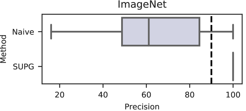
Figure 1: Box plot of achieved precisions of naive sampling from recent work [44, 47] and our improved algorithm. Over 100 runs targeting a precision of 90%, the naive algorithm returns precisions as low as 65% for over half the runs. In contrast, our algorithms (SUPG) achieve the precision target with high probability.

First, given the budget, using an unreliable proxy model can result in false negatives or positives, making it difficult to guarantee the accuracy of query results. Existing systems do not provide guarantees on the accuracy. In fact they can fail unpredictably and catastrophically, providing results with low accuracy a significant fraction of the time [44, 43, 47, 13, 5, 39]. For example, when users request a precision of at least 90%, over repeated runs, existing systems return results with less than 65% precision over half the time, with some runs low as 20% (Figure 1). These failures can be even worse in the face of shifting data distributions, i.e., model drift (Section 6.2). Such failures are unacceptable in production deployment and for scientific inference.

Second, existing systems do not make efficient use of limited oracle labels to maximize the quality of query results. To avoid vacuous results (e.g., achieving a perfect recall by returning the whole dataset will have poor precision), NoScope, probabilistic predicates, and other recent work uniformly sample records to label with the oracle in order to decide on the final set of records to return. We show that this is wasteful. In the common case where records matching the predicate are rare, the vast majority of uniformly sampled records will be negatives, with too few positives. Thus, naively extending existing techniques to have accuracy guarantees can fail to maintain high result quality given these uninformative labels.

In response we develop novel algorithms that provide both statistical guarantees and efficient use of oracle labels for approximate selection. We further develop query semantics for the two settings we consider: the recall target and precision target settings.

Accuracy guarantees. To address the challenge of guarantees on failure probability, we first define probabilistic guarantees for two classes of approximate selection queries. We have found that users are interested in queries targeting a minimum recall (RT queries) or targeting a minimum precision (PT queries), subject to an oracle label budget and a failure probability on the query returning an invalid result (Section 3). For instances, the biologist are interested in 90% recall and a failure probability of at most 5%.

We develop novel algorithms (SUPG algorithms) that provide these guarantees by using the oracle budget to randomly sample records to label, and estimating a proxy confidence threshold $\tau$ for which it is safe to return all records with proxy score above $\tau$. Naive use of uniform sampling will not account for the probability that there is a deviation between observed labels and proxy scores, and will further introduce multiple hypothesis testing issues. This will result in a high probability of failure. In response, we make careful use of confidence intervals and multiple hypotheses corrections to ensure that the failure probability is controlled.

Oracle sample efficiency. A key challenge is deciding which data points to label with the oracle given the limited budget: as we show, uniform sampling is inefficient. Instead, we develop novel, optimal importance sampling estimators that use of the correlation between the proxy and the oracle, while taking into account possible mismatches between the binary oracle and continuous proxy. Intuitively, importance sampling upweights the probability of sampling data points with high proxy scores, which are more likely to contain the events of interest.

However, naive use of importance sampling results in poor performance when sampling according to proxy scores. Using a variance decomposition, we find that a standard approach for obtaining importance weights (i.e., using weights proportional to the proxy) is suboptimal and, excluding edge cases, performs no better than uniform random sampling.

Instead, we show that sampling proportional to the square root of the proxy scores allows for more efficient estimates of the proxy threshold when the proxy scores are confident and reliable (Section 5.3.1). For precision target queries, we additionally extend importance sampling to use a two-stage sampling procedure. In the first stage, our algorithm estimates a safe interval to further sample. In the second stage, our algorithm samples directly from this range, which we show greatly improves sample efficiency.

Careless of use of importance sampling can hurt result quality when used with poor proxy models. If proxy scores are uncorrelated with the true labels, importance sampling will in fact increase the variance of sampling. To address these issues, we defensively incorporate uniform samples to guard against situations where the proxy may be adversarial [49]. This procedure still maintains the probabilistic accuracy guarantees.

We implement and evaluate these algorithms on real and synthetic datasets and show that our algorithms achieve desired accuracy guarantees, even in the presence of model drift. We further show that our algorithms outperform alternative methods in providing higher result quality, by as much as 30$\times$ higher recall/precision under precision/recall constraints respectively.

In summary, our contributions are:

1. We introduce semantics for approximate selection queries with probabilistic accuracy guarantees under a limited oracle budget.

2. We develop algorithms for approximate selection queries that satisfy bounded failure probabilities while making efficient use of the oracle labels.

3. We implement and evaluate our algorithms on six real-world and synthetic datasets, showing up to 30$\times$ improvements in quality and consistent ability to achieve target accuracies.

2 Use Cases

To provide additional context and motivation for approximate selection queries, we describe scenarios where statistically efficient queries with guarantees are essential. Each scenario is informed by discussions with academic and industry collaborations.

2.1 Biological Discovery

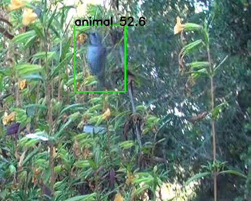
(a) Hummingbird present

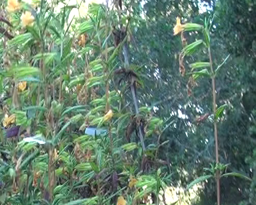
(b) No hummingbirds

Figure 2: Sample matching (a) and non-matching (b) frames for a selection query over a video stream used by our biologist collaborators. Only a small ($<.1\%$) fraction of frames have hummingbirds present and match the filter predicate, making manual inspection difficult. DNNs can serve as proxies to identify hummingbirds as shown in (a), but the confidence scores can be unreliable.

Scenario. We are actively collaborating with the Fukami lab at Stanford University, who study bacterial colonies in flowers [52]. The Fukami lab is interested in hummingbirds that move bacteria between flowers as they feed, as this bacterial movement can affect both the micro-ecology of the flowers and later hummingbird feeding patterns. To study such phenomena, they have collected videos of bushes with tagged flowers at the Jasper Ridge biological preserve. They have recorded six views of the scene with a total of approximately 9 months of video. At 60 fps, this is approximately 1.4B frames of video. To perform downstream analyses, our collaborators want to select all frames in the video that contain hummingbirds. Due to the rarity of hummingbird appearances ($<0.1\%$) and the length of the video, they have been unable to manually review the video in its entirety. We illustrate the challenge in Figure 2.

Proxy model. Prior to our collaboration, the Fukami lab used motion detectors as a proxy for identifying frames with birds. However, the motion detectors have severe limitations: their precision is extremely low (approximately 2%) and they do not cover the full field of view of the bush. As an alternative, we are actively using DNN object detector models to identify hummingbirds directly from frames of the video [31, 8]. These DNN models are more precise than motion detectors, and can provide a confidence score in addition to a Boolean predicate result.

During discussion with the Fukami lab, we have found that the scientists require high probability guarantees on recall, as finding the majority of hummingbirds is critical for downstream analysis. Furthermore, they are interested in improving precision relative to the motion detectors. The scientists have specified that they need a recall of at least 90% and a precision that is as high as possible, ideally above 20%.

⬇

SELECT * FROM table_name

WHERE filter_predicate

ORACLE LIMIT o

USING proxy_estimates

[RECALL | PRECISION] TARGET t

WITH PROBABILITY p

Figure 3: Syntax for specifying approximate selection queries. Users provide a precision or recall target, a budget for the number of oracle predicate evaluations, and a probability of success.

2.2 Autonomous Vehicle Training

Scenario. An autonomous vehicle company may collect data in a new area. To train the DNNs used in the vehicle, the company may extract point cloud or visual data and use a labeling service to label pedestrians. Unfortunately, labeling services are known to be noisy and may not label pedestrians even when they are visible [23].

To ensure that all pedestrians are labeled, an analyst may wish to select all frames where pedestrians are present but are not annotated in the labeled data. However, as autonomous vehicle fleets collect enormous amounts of data (petabytes per day), the analyst is not able to manually inspect all the data.

Proxy model. As the proxy model, the analyst can use an object detection method and remove boxes that are in the labeled dataset. The analyst can then use the confidences from the remaining boxes from the object detection as the proxy scores.

As this is a mission-critical setting, the analyst is interested in guarantees on recall. Missing pedestrians in the labeled dataset can transfer to missing pedestrians at deployment time, which can cause fatal accidents.

We further note that the analyst may also be interested in using other proxies, such as 3D detections from LIDAR data. In this work, we only study the use of a single proxy model, but we see extending our algorithms to multiple proxy models as an exciting area of future work (Section 8).

We note that this scenario is not limited to autonomous vehicles but can apply to other scenarios where curating high quality machine learning datasets is of paramount concern.

2.3 Legal Discovery and Analysis

Scenario. Lawyers are often tasked with analyzing large corpora of data, e.g., they may inspect a corpus of emails as part of legal discovery, or may be tasked to analyze if private information was leaked in a data breach [40, 41]. This process is expensive as hiring contract lawyers to manually inspect documents is time consuming and expensive. As a result, a number of companies are interested in leveraging automatic methods to select all records that match sensitive named entities or reference relevant legal concepts.

Proxy model. As the proxy model, an analyst may fine-tune a sophisticated language understanding model, such as BERT [22]. The analyst can deploy this model over the corpus of text data and extract noisy labels to help the lawyers. For sensitive issues, companies would benefit from tools that can provide either recall or precision guarantees depending on the scenario.

3 Approximate Selection Queries

We introduce our definitions for our approximate selection queries (SUPG queries), describe the probabilistic guarantees they respect, and define metrics for comparing the quality of the results.

3.1 Query Semantics

A SUPG query is a selection query for set of records matching a predicate, with syntax given in Figure 3. Unlike much of the existing work in approximate query processing, SUPG queries return a set of matching records rather than a scalar or vector aggregate [34, 4]. We defined these semantics to formalize a common class of queries our collaborators and industrial contacts are interested in executing.

The query specifies a filter predicate given by a “ground truth” oracle, as well as a limited budget of total calls to the oracle over the course of query execution. We use the term oracle to refer to any expensive predicate the user wishes to approximate. In some cases, the oracle may be an expensive DNN (e.g., the highly accurate Mask R-CNN [31]) that may not exactly match the ground truth labels that a human labeler would provide. However, the use of proxies to approximate powerful deep learning models is common in the literature [44, 43, 47, 39, 5], so we study how to provide guarantees in applications that use a larger DNN as an oracle.

Since oracle usage is limited, queries also specify proxy confidence scores for whether a record matches the predicate. The proxy scores must be correlated with the probability that a record matches the filter predicate to be useful. Nonetheless, our novel algorithms will return valid results even if proxy scores are not correlated.

The accuracy of the set of results can be measured using either recall (the fraction of true matches returned) or precision (the fraction of returned results that are true matches). Based on the application, a user can specify either a minimum recall or precision target as well as a desired probability of achieving this target. We refer to these two options as precision target (PT) and recall target (RT) queries. As an example, consider the following RT query:

⬇

SELECT * FROM hummingbird_video

WHERE HUMMINGBIRD_PRESENT(frame) = True

ORACLE LIMIT 10,000

USING DNN_CLASSIFIER(frame) = "hummingbird"

RECALL TARGET 95%

WITH PROBABILITY 95%

where both HUMMINGBIRD_PRESENT and DNN_CLASSIFIER are user-defined functions (UDFs). This query selects the frames of the video that contains a hummingbird with recall at least 95%, using at most 10,000 oracle evaluations, and a failure probability of at most 5%, using confidence probabilities from a DNN classifier as a proxy. The oracle could be a human labeler or expensive DNN.

Finally, we note that some queries may require both a recall and precision target. Unfortunately, jointly achieving both targets may require an unbounded number of oracle queries. Since all use cases we consider have limited budgets, we defer our discussion of these queries to an extended version of this paper [45].

3.2 Probabilistic Guarantees

More formally, a SUPG query $\mathcal{Q}$ is defined by an oracle predicate $O(x)\in\{0,1\}$ over a set of records $x$ from a dataset $\mathcal{D}$. The ideal result for the query would be the matching records $O^{+}\coloneqq\{x\in\mathcal{D}:O(x)=1\}$. However, since the oracle is assumed to be expensive, the query specifies a budget of $s$ calls to the oracle $O(x)$, as well as a proxy model $A(x)\in[0,1]$ whose use is unrestricted. The query specifies a minimum recall or precision target $\gamma$. Then, a valid query result would be a set of records $\mathcal{R}$ such that $\text{Precision}(\mathcal{R})>\gamma_{p}$ or $\text{Recall}(\mathcal{R})>\gamma_{r}$ depending on the query type. Recall that

$$\text{Precision}(\mathcal{R})\coloneqq\frac{|\mathcal{R}\cap O^{+}|}{|\mathcal{R}|}\qquad\text{Recall}(\mathcal{R})\coloneqq\frac{|\mathcal{R}\cap O^{+}|}{|O^{+}|}.$$

A SUPG query further specifies a failure probability $\delta$. Many precision or recall targets $\gamma$ may be impossible to achieve deterministically given a limited budget of $s$ calls to the oracle, as they require exhaustive search. Thus, it is common in approximate query processing and statistical inference to use randomized procedures with a bounded failure probability [20]. A randomized algorithm satisfies the guarantees in $\mathcal{Q}$ if it produces valid results $\mathcal{R}$ with high probability. That is, for PT queries:

$$\Pr[\text{Precision}(\mathcal{R})\geq\gamma_{p}]\geq 1-\delta$$ (1)

and for RT queries:

$$\Pr[\text{Recall}(\mathcal{R})\geq\gamma_{r}]\geq 1-\delta.$$ (2)

These high probability guarantees are much stronger than merely achieving an average recall or precision as many existing systems do [44, 47, 5, 39]. For example, in Figure 6 we illustrate the true recall provided for queries targeting 90% recall to NoScope system, and compare them with the recall provided by SUPG which satisfies the stronger guarantee in Equation 2. NoScope only achieves the target recall approximately half of the time, with many runs failing to achieve the recall target by a significant margin. Such results that fail to achieve the recall target would have a significant negative impact on downstream statistical analyses.

3.3 Result Quality

Since SUPG queries only specify a target for either precision or recall (the target metric), there are many valid results for a given query which may be more or less useful. For instance, if a user targets $99\%$ recall the entire dataset is always a valid result, even though this may not be useful to the user. In this case, it would be more useful to return a smaller set of records to minimize false positives. Similarly, if a user targets high precision the empty set is always a valid result, and is equally useless. Thus, we define selection query quality in this paper as follows:

Definition 1.

For RT/PT queries, a higher quality result is one with higher precision/recall, respectively.

There is an inherent trade-off between returning valid results and maximizing result quality, analogous to the trade-off between maximizing precision and maximizing recall in binary classification [28, 11], but efficient use of oracle labels will allow us to develop more efficient importance sampling based query techniques.

4 Algorithm Overview

In this section, we describe the system setting that our SUPG algorithms operate in, and outline the major stages in the algorithm: sampling oracle labels, choosing a proxy threshold, and returning a set of data record results.

4.1 Operational Architecture

Our algorithms are designed for batch query systems that perform selection on datasets of existing records. Users can issue queries over the data with specified predicates and parameters as described earlier. Note that the oracle and proxy models used to evaluate the filter predicate are provided by the user as UDFs (callback functions) and are not inferred by the system. Thus, a user must provide either a ground truth DNN or interface to obtain human input as an oracle, as well as pre-trained inexpensive proxy models. In practice, one can provide user interfaces for interactively requesting human labels [1] as well as scripts for automatically constructing smaller proxy models from an existing oracle [44, 47], though those are outside the scope of this paper.

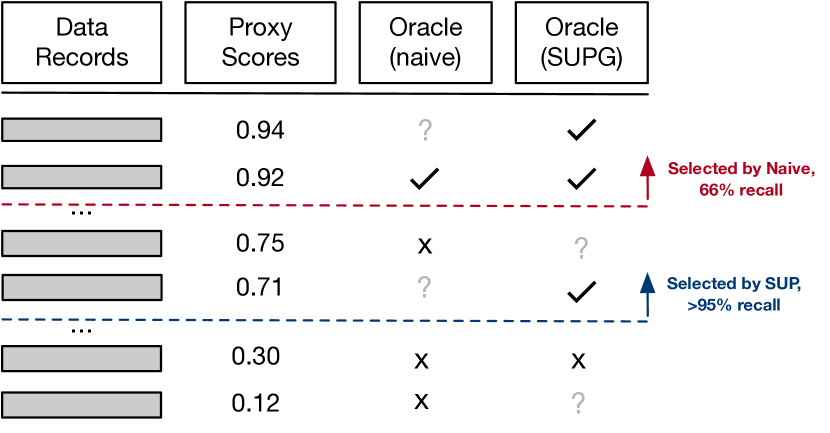
Figure 4: Our SUPG algorithms uses sampled oracle labels and proxy scores to identify a subset of records that satisfy a recall or precision target with high probability. Naive selection methods, as used by recent work, would make less efficient use of limited oracle labels, and provide weaker guarantees: in fact they often fail to achieve a target recall or precision.

We illustrate how SUPG uses oracle and proxy models in Figure 4. For all query types, SUPG first executes the proxy model over the complete set of records $\mathcal{D}$ as we assume the proxy model is cheap relative to the oracle model. Then, SUPG samples a set $\mathcal{S}$ of $s$ records to label using the oracle model. The choice of which records to label using the oracle is done adaptively, that is, the choice of samples may depend on the results of previous oracle calls for a given query.

function SUPGQuery($\mathcal{D}$, $A$, $O$)

     $\mathcal{S}\leftarrow\texttt{SampleOracle}(\mathcal{D})$

     $\tau\leftarrow\texttt{EstimateTau}(\mathcal{S})$

     $\mathcal{R}_{1}\leftarrow\{x:x\in\mathcal{S}\wedge O(x)=1\}$

     $\mathcal{R}_{2}\leftarrow\{x:x\ \in\mathcal{D}\wedge A(x)\geq\tau\}$

     return $\mathcal{R}_{1}\cup\mathcal{R}_{2}$

Algorithm 1 SUPG query processing

We summarize this sequence of operations SUPG uses to return query results in Algorithm 1. After calling the oracle to obtain predicate labels over a sample $\mathcal{S}$, SUPG sets a proxy score threshold $\tau$ and then returns results $\mathcal{R}$ that consist of both labeled records in $\mathcal{S}$ matching the oracle predicate as well as records with proxy scores above the threshold $\tau$. $\tau$ is tuned so that the final results $\mathcal{R}$ satisfy minimum recall or precision targets with high probability, and we describe the process for setting $\tau$ below.

4.2 Choosing a Proxy Threshold

Since the proxy scores are the only source of information on the query predicate besides the oracle model, SUPG naturally returns records corresponding to all records with scores above a threshold $\tau$. This strategy is known to be optimal in the context of retrieval and ranking as long as proxy scores grow monotonically with an underlying probability that the record matches a predicate [48]. We have observed in practice that this is approximately true for proxy models by computing empirical match rates for bucketed ranges of the proxy scores, so we use this as the default strategy in SUPG. For proxy models that are completely uncorrelated or have non-monotonic relationships with the oracle, all algorithms using proxies will have increasingly poor quality, but SUPG will still provide accuracy guarantees.

Thus, the key task is selecting the threshold $\tau$ to maintain result validity while maximizing result quality. This threshold must be set at query time since the relation between proxy scores and the predicate is unknown, especially when production model drift is an issue. Existing systems have often relied on pre-set thresholds determined ahead of time, which we show in Section 6.2 can lead to severe violations of result validity.

One naive strategy for selecting $\tau$ at query time is to uniform randomly sample records to label with the oracle until the budget is exhausted, and then select $\tau$ that achieves a target accuracy over the sample. However, this strategy on its own does not provide strong accuracy guarantees or make efficient use of the sample budget. Thus, in Section 5 we introduce more sophisticated methods for sampling records and estimating the threshold: that is, implementations of SampleOracle and EstimateTau.

Table 1: Notation Summary

Symbol	Description
$O(x)$	Oracle predicate value
$A(x)$	Proxy confidence score
$\delta$	Failure probability
$\gamma$	Target Recall / Precision
$\tau$	Proxy score threshold for selection
$\mathcal{S}$	Records sampled for oracle evaluation

5 Estimating proxy thresholds

Recall that SUPG selects all records with proxy scores above a threshold $\tau$. Denote this set of records

$$\mathcal{D}(\tau)\coloneqq\{x:A(x)\geq\tau\}.$$

SUPG query accuracy thus critically depends on the choice of $\tau$. In this section we describe our algorithms for estimating a threshold that can guarantee valid results with high probability, while maximizing result quality. While precision target (PT) and recall target (RT) queries require slightly different threshold estimation routines, in both cases SUPG samples records to label with the oracle. Using this sample, SUPG will select a threshold $\tau$ that achieves the target metric on the dataset $\mathcal{D}$ with high probability.

In order to explain our algorithms and compare them with existing work, we will also describe a number of baseline techniques which do not provide statistical guarantees, and do not make efficient use of oracle labels to improve result quality.

We now describe baselines without guarantees, how to correct these baselines for statistical guarantees on failure probability, and finally our novel importance sampling algorithms.

5.1 Baselines Without Guarantees

The simplest strategy for estimating a valid threshold would be to take a uniform i.i.d. random sample of records $\mathcal{S}$, label the records with the oracle, and then use $\mathcal{S}$ as an exact representative of the dataset $\mathcal{D}$ when choosing a threshold. This is the approach used by probabilistic predicates and NoScope [44, 47], and we call this approach U-NoCI because it uses a uniform sample and does not account for failure probabilities using confidence intervals (CI). Let $\text{Recall}_{\mathcal{S}}(\tau)$ and $\text{Precision}_{\mathcal{S}}(\tau)$ denote the empirical recall and precision for the sampled data $\mathcal{S}$, and $1_{c}$ denote the indicator function that condition $c$ holds:

$$\text{Recall}_{\mathcal{S}}(\tau) \coloneqq\frac{\sum_{x\in\mathcal{S}}1_{A(x)\geq\tau}O(x)}{\sum_{x\in\mathcal{S}}O(x)}$$ (3)

$$\text{Precision}_{\mathcal{S}}(\tau) \coloneqq\frac{\sum_{x\in\mathcal{S}}1_{A(x)\geq\tau}O(x)}{|\mathcal{S}|}.$$ (4)

The U-NoCI-P approach maximizes result quality subject to constraints on these empirical recall and precision estimates. For PT queries this results in finding the minimal $\tau$ (minimizing false negatives) that achieves the target metric on $\mathcal{S}$, and for RT queries this results in finding the maximum $\tau$ (minimizing false positives). Formally this is defined as,

$$\tau_{\text{{U}-{NoCI}-{P}}}(\mathcal{S}) =\min\{\tau:\text{Precision}_{\mathcal{S}}(\tau)\geq\gamma\}$$ (5)

$$\tau_{\text{{U}-{NoCI}-{R}}}(\mathcal{S}) =\max\{\tau:\text{Recall}_{\mathcal{S}}(\tau)\geq\gamma\}.$$ (6)

However, we have no guarantee that the thresholds selected in this way will provide valid results on the complete dataset, due to the random variance in choosing a threshold based on the limited sample. We empirically show that such algorithms fail to achieve targets up to 80% of the time in Section 6.2.

5.2 Guarantees through Confidence Intervals

In order to provide probabilistic guarantees, we form confidence intervals over $\tau$ and take the appropriate upper or lower bound.

Normal approximation. In Lemma 1 we describe an asymptotic bound relating sample averages to population averages, allowing us to bound the discrepancy between recall and precision achieved on $\mathcal{S}$ vs $\mathcal{D}$. This approximation is commonly used in the approximate query processing literature [34, 29, 3].

For ease of notation we will refer to the upper and lower bounds provided by Lemma 1 using helper functions

$$\text{UB}(\mu,\sigma,s,\delta) \coloneqq\mu+\frac{\sigma}{\sqrt{s}}\sqrt{2\log{\frac{1}{\delta}}}$$ (7)

$$\text{LB}(\mu,\sigma,s,\delta) \coloneqq\mu-\frac{\sigma}{\sqrt{s}}\sqrt{2\log{\frac{1}{\delta}}}.$$ (8)

Lemma 1

Let $\mathcal{S}$ be a set of $s$ i.i.d. random variables $x\sim\mathcal{X}$ with mean $\mu$ and finite variance $\sigma^{2}$ and sample mean $\hat{\mu}$. Then,

$$\lim_{s\rightarrow\infty}\Pr\left[\hat{\mu}\geq\text{UB}(\mu,\sigma,s,\delta)\right] \leq\delta$$

and

$$\lim_{s\rightarrow\infty}\Pr\left[\hat{\mu}\leq\text{LB}(\mu,\sigma,s,\delta)\right] \leq\delta.$$

Lemma 1 defines the expected variation in recall and precision estimates as $s$ grows large, and follows from the Central Limit Theorem [56]. Using this, we can select conservative thresholds that with high probability still provide valid results on the underlying dataset $\mathcal{D}$. Though this bound is an asymptotic result for large $s$, quantitative convergence rates for such statistics are known to be fast [9] and we found that this approach provides the appropriate probabilistic guarantees at sample sizes $s>100$.

Other confidence intervals. Throughout, we use Lemma 1 to compute confidence intervals. There are other methods to compute confidence intervals, e.g., the bootstrap [24], Hoeffding’s inequality [37], and “exact” methods for Binomial proportions (Clopper-Pearson interval) [19]. We show that the normal approximation matches or outperforms alternative methods of computing confidence intervals (Section 6.4). Since the normal approximation is straightforward to implement and applies to both uniform and importance sampling we use it throughout.

We will now describe baseline uniform sampling based methods for estimating $\tau$ in both RT and PT queries.

5.2.1 Recall Target

For recall target queries, we want to estimate a threshold $\tau$ such that $\text{Recall}_{\mathcal{D}}(\tau)\geq\gamma$ with probability at least $1-\delta$. To maximize result quality we would further like to make $\tau$ as large as possible. We present the pseudocode for a threshold selection routine U-CI-R that provides guarantees on recall in Algorithm 2.

Note that Algorithm 2 finds a cutoff $\tau$ that achieves a conservative recall of $\gamma^{\prime}$ on $\mathcal{S}$ instead of the target recall $\gamma$. This inflated recall target accounts for the potential random variation from forming the threshold on $\mathcal{S}$ rather than $\mathcal{D}$.

Validity justification. Let $\tau_{o}$ be the largest threshold providing valid recall on $\mathcal{D}$:

$$\tau_{o}\coloneqq\max\{\tau:\text{Recall}_{\mathcal{D}}(\tau)\geq\gamma\}$$

If $\text{Recall}_{\mathcal{S}}(\tau_{o})\leq\gamma^{\prime}$ then Algorithm 1 will select a threshold $\tau^{\prime}$ where $\tau^{\prime}\leq\tau_{o}$ since recall varies inversely with the threshold. Then, $\text{Recall}_{\mathcal{D}}(\tau^{\prime})\geq\text{Recall}_{\mathcal{D}}(\tau)\geq\gamma$ and the results derived from $\tau^{\prime}$ would be valid.

It remains to show that with probability $1-\delta$, $\gamma^{\prime}$ satisfies:

$$\text{Recall}_{\mathcal{S}}(\tau_{o})\leq\gamma^{\prime}.$$ (9)

Let $Z_{1}(\tau),Z_{2}(\tau)$ be sample indicator random variables for matching records above and below $\tau_{o}$, corresponding to the samples in $\mathcal{S}$.

$$Z_{1}(\tau) \coloneqq\{1_{A(x)\geq\tau}O(x):x\in\mathcal{S}\}$$

$$Z_{2}(\tau) \coloneqq\{1_{A(x)<\tau}O(x):x\in\mathcal{S}\}.$$

Note that $\frac{\hat{\mu}_{Z_{1}(\tau)}}{\hat{\mu}_{Z_{1}(\tau)}+\hat{\mu}_{Z_{2}(\tau)}}=\text{Recall}_{\mathcal{S}}(\tau)$, which increases with $\hat{\mu}_{Z_{1}(\tau)}$ and decreases with $\hat{\mu}_{Z_{2}(\tau)}$. Thus, if we let

$$\gamma^{*}=\frac{\text{UB}(\mu_{Z_{1}(\tau_{o})},\sigma_{Z_{1}(\tau_{o})},s,\frac{\delta}{2})}{\text{UB}(\mu_{Z_{1}(\tau_{o})},\sigma_{Z_{1}(\tau_{o})},s,\frac{\delta}{2})+\text{LB}(\mu_{Z_{2}(\tau_{o})},\sigma_{Z_{2}(\tau_{o})},s,\frac{\delta}{2})}$$

then asymptotically as $s\to\infty$ Lemma 1 ensures $\text{Recall}_{\mathcal{S}}(\tau_{o})=\frac{\hat{\mu}_{Z_{1}(\tau_{o})}}{\hat{\mu}_{Z_{1}(\tau_{o})}+\hat{\mu}_{Z_{2}(\tau_{o})}}\leq\gamma^{*}$ with probability $1-\delta$. $\gamma^{*}$ is not computable from our sample so we use plug-in estimates for $\tau_{o}$, $\mu$, and $\sigma$ to estimate a $\gamma^{\prime}\rightarrow\gamma^{*}$ as $s\rightarrow\infty$.

5.2.2 Precision Target

For precision target queries, we want to estimate a threshold $\tau$ such that $\text{Precision}_{\mathcal{D}}(\tau)\geq\gamma$ with high probability. To maximize result quality (i.e., maximize recall), we would further like to make $\tau$ as small as possible.

Unlike for recall target queries, there is no monotonic relationship between $\text{Precision}_{\mathcal{D}}(\tau)$ and $\tau$: $\text{Precision}_{\mathcal{D}}(\tau_{1})$ may be greater than $\text{Precision}_{\mathcal{D}}(\tau_{2})$ even if $\tau_{1}<\tau_{2}$. Thus, for PT queries we calculate lower bounds on the precision provided by a large set of candidate thresholds $\tau$, and return the smallest candidate threshold that provides results with precision above the target.

function $\tau_{\text{{U}-{CI}-{R}}}$($\mathcal{D}$)

     $\mathcal{S}\leftarrow\text{UniformSample}(\mathcal{D},s)$

     $\hat{\tau}_{o}\leftarrow\max\{\tau:\text{Recall}_{\mathcal{S}}(\tau)\geq\gamma\}$

     $Z_{1}\leftarrow\{1_{A(x)\geq\hat{\tau}_{o}}O(x):x\in\mathcal{S}\}$

     $Z_{2}\leftarrow\{1_{A(x)<\hat{\tau}_{o}}O(x):x\in\mathcal{S}\}$

     $\gamma^{\prime}\leftarrow\frac{\text{UB}(\hat{\mu}_{z_{1}},\hat{\sigma}_{z_{1}},s,\delta/2)}{\text{UB}(\hat{\mu}_{z_{1}},\hat{\sigma}_{z_{1}},s,\delta/2)+\text{LB}(\hat{\mu}_{z_{2}},\hat{\sigma}_{z_{2}},s,\delta/2)}$

     $\tau^{\prime}\leftarrow\max\{\tau:\text{Recall}_{\mathcal{S}}(\tau)\geq\gamma^{\prime}\}$

     return $\tau^{\prime}$

Algorithm 2 Uniform threshold estimation (RT)

$m\leftarrow 100$ $\triangleright$ Minimum step size

function $\tau_{\textsc{U}-\textsc{CI}-\textsc{P}}$($\mathcal{D}$)

     $\mathcal{S}\leftarrow\text{UniformSample}(\mathcal{D},s)$

     $A_{\mathcal{S}}\leftarrow\text{Sort}(\{A(x):x\in\mathcal{S}\})$

     $M\leftarrow\lceil s/m\rceil$

     $\text{Candidates}\leftarrow\{\}$

     for $i\leftarrow m,2m,\dots,s$ do

         $\tau\leftarrow A_{\mathcal{S}}[i]$

         $Z\leftarrow\{O(x):x\in\mathcal{S}\wedge A(x)\geq\tau\}$

         $p_{l}\leftarrow\text{LB}(\hat{\mu}_{Z},\hat{\sigma}_{Z},|Z|,\delta/M)$ $\triangleright$ Precision Bound

         if $p_{l}>\gamma$ then

              $\text{Candidates}\leftarrow\text{Candidates}\cup\{\tau\}$               

     return $\min_{\tau}\text{Candidates}$

Algorithm 3 Uniform threshold estimation (PT)

We provide pseudocode for U-CI-R which uses confidence intervals over a uniform sample (Algorithm 3). Since the procedure uses Lemma 1 $M$ times by union bound we need each usage to hold with probability $1-\delta/M$ for the final returned threshold to be valid with probability $1-\delta$.

Validity justification. Let

$$Z(\tau)=\{O(x):x\in\mathcal{S}\wedge A(x)\geq\tau\},$$

then $\hat{\mu}_{Z(\tau)}=\text{Precision}_{\mathcal{S}}(\tau)$ and $\mu_{Z(\tau)}=\text{Precision}_{\mathcal{D}}(\tau).$ Asymptotically by Lemma 1, with probability $1-\delta/M$

$$\text{LB}(\hat{\mu}_{Z(\tau)},\sigma_{Z(\tau)},|Z(\tau)|,\delta/M)\leq\mu_{Z(\tau)}.$$

By the union bound, as long as each $\tau$ in the Candidate set has $\text{LB}(\hat{\mu}_{Z(\tau)},\sigma_{Z(\tau)},|Z(\tau)|,\delta/M)>\gamma$, the precision for each of the candidates over the dataset also exceeds $\gamma$. Since we do not know $\sigma$, in Algorithm 3 we use sample plug-in estimates for $\sigma_{Z(\tau)}$. Alternatively one could use a t-test (both are asymptotically valid).

5.3 Importance Sampling

The U-CI routines for estimating $\tau$ in Algorithms 2 and 3 provide valid results with probability $1-\delta$. However if the random sample chosen for oracle labeling $\mathcal{S}$ is uninformative, the confidence bounds we use will be wide and the threshold estimation routines will return results that have lower quality in order to provide valid results. Thus, we explain how SUPG uses importance sampling to select a set of points that improve upon uniform sampling. We refer to these more efficient routines as IS-CI estimators.

Importance sampling chooses records $x$ with replacement from the dataset $\mathcal{D}$ with weighted probabilities $w(x)$ as opposed to uniformly with base probability $u(x)$. One can compute the expected value of a quantity $f(x)$ with reduced variance by then sampling according to $w$ rather than $u$ and using the reweighting identity:

$$\mathop{\mathbb{E}}_{x\sim u}[f(x)]=\mathop{\mathbb{E}}_{x\sim w}\left[f(x)\frac{u(x)}{w(x)}\right].$$ (10)

Abbreviating the reweighting factor as $m(x)\coloneqq u(x)/w(x)$, we can then define reweighted estimates for recall and precision on a weighted sample $\mathcal{S}_{w}$:

$$\text{Recall}_{\mathcal{S}_{w}}(\tau) \coloneqq\frac{\sum_{x\in\mathcal{S}}1_{A(x)\geq\tau}O(x)m(x)}{\sum_{x\in\mathcal{S}_{w}}O(x)m(x)}$$ (11)

$$\text{Precision}_{\mathcal{S}_{w}}(\tau) \coloneqq\frac{\sum_{x\in\mathcal{S}}1_{A(x)\geq\tau}O(x)m(x)}{\sum_{x\in\mathcal{S}_{w}}m(x)}$$ (12)

If we can reduce the variance of these estimates, we can use the tighter bounds to improve the quality of the results at a given recall or precision target.

The optimal choice of $w(x)$ for the standard importance sampling setting is $w(x)\propto f(x)u(x)$ [56]. However, this assumes $f(x)$ is a known function. In our setting, we want $f(x)=1_{A(x)\geq\tau}O(x)$ which is both stochastic and a priori unknown. This prevents us from directly applying traditional importance sampling weights based on $f(x)$. Instead, we can use the proxy $A(x)$ to define sampling weights.

Our approach solves for the optimal sample weights for proxies that are highly correlated with the oracle, i.e. calibrated with $A(x)=\Pr_{x\sim u}[O(x)=1|A(x)]$. In practice this will not hold exactly, but as long as the proxy scores are approximately proportional to the probability we can use them to derive useful sample weights. We show in Section 5.3.1 that the optimal weights which minimize the variance are proportional to $\sqrt{A(x)1_{A(x)\geq\tau}}u(x)$. To guard against situations where the proxy could be inaccurate, we defensively mix a uniform distribution with these optimal weights in our algorithms [49].

Note that the validity of our results does not depend on the proxy being calibrated, but this importance sampling scheme allows us to obtain lower variance threshold estimates and thus more efficient query results when the proxy is close to calibrated.

Recall target. For recall target queries, we extend Algorithm 2 to use weighted samples according to Theorem 1. We use the weights to optimize the variance of $E[O(x)]$ as a proxy for reducing the variance of $E[1_{A(x)\geq\tau_{o}}O(x)]$ and $E[1_{A(x)<\tau_{o}}O(x)]$. We present this weighted method, IS-CI-R, in Algorithm 4. The justification for high probability validity is the same as before.

function $\tau_{\text{{IS}-{CI}-{R}}}$($\mathcal{D}$)

     $\vec{w}\leftarrow\{\sqrt{A(x)}:x\in\mathcal{D}\}$

     $\vec{w}\leftarrow.9\cdot\vec{w}/\|\vec{w}\|_{1}+.1\cdot\vec{1}/|\mathcal{D}|$ $\triangleright$ Defensive Mixing

     $\mathcal{S}\leftarrow\text{WeightedSample}(\mathcal{D},\vec{w},s)$

     $m(x)\leftarrow\frac{1/|\mathcal{D}|}{w(x)}$

     $\tau_{o}\leftarrow\max\{\tau:\text{Recall}_{\mathcal{S}_{w}}(\tau)\geq\gamma\}$

     $\hat{z}_{1}\leftarrow\{1_{A(x)\geq\tau_{o}}O(x)m(x):x\in\mathcal{S}\}$

     $\hat{z}_{2}\leftarrow\{1_{A(x)<\tau_{o}}O(x)m(x):x\in\mathcal{S}\}$

     $\gamma^{\prime}\leftarrow\frac{\text{UB}(\hat{\mu}_{z_{1}},\hat{\sigma}_{z_{1}},s,\delta/2)}{\text{UB}(\hat{\mu}_{z_{1}},\hat{\sigma}_{z_{1}},s,\delta/2)+\text{LB}(\hat{\mu}_{z_{2}},\hat{\sigma}_{z_{2}},s,\delta/2)}$

     $\tau^{\prime}\leftarrow\max\{\tau:\text{Recall}_{\mathcal{S}_{w}}(\tau)\geq\gamma^{\prime}\}$

     return $\tau^{\prime}$

Algorithm 4 Importance threshold estimation (RT)

Precision target. For PT queries we can combine Theorem 1 with an additional observation: if we know there are at most $n_{\text{match}}$ positive matching records in $\mathcal{D}$, then there is no need to consider thresholds lower than the $n_{\text{match}}/\gamma$-th highest proxy score in $\mathcal{D}$, since any lower thresholds cannot achieve a precision of $\gamma$. SUPG thus devotes half of the oracle sample budget to estimating the upper bound $n_{\text{match}}$ and the remaining half for running a weighted version of Algorithm 3 on candidate thresholds. We present this two-stage weighted sampling algorithm, IS-CI-P, in Algorithm 5.

$m\leftarrow 100$ $\triangleright$ Minimum step size

function $\tau_{\text{{IS}-{CI}-{P}}}$($\mathcal{D}$)

     $\vec{w}\leftarrow\{\sqrt{A(x)}:x\in\mathcal{D}\}$

     $\vec{w}\leftarrow.9\cdot\vec{w}/\|\vec{w}\|_{1}+.1\cdot\vec{1}/|\mathcal{D}|$ $\triangleright$ Defensive Mixing

     $\mathcal{S}_{0}\leftarrow\text{WeightedSample}(\mathcal{D},w,s/2)$ $\triangleright$ Stage 1

     $m(x)\leftarrow\frac{1/|\mathcal{D}|}{w(x)}$

     $Z\leftarrow\{O(x)m(x):x\in\mathcal{S}_{0}\}$

     $n_{\text{match}}\leftarrow|\mathcal{D}|\cdot\text{UB}(\hat{\mu}_{Z},\hat{\sigma}_{Z},s/2,\delta/2)$

     $A\leftarrow\text{SortDescending}(\{A(x):x\in\mathcal{D}\})$

     $\mathcal{D}^{\prime}\leftarrow\{x:A(x)\geq A[n_{\text{match}}/\gamma]\}$

     $\mathcal{S}_{1}\leftarrow\text{WeightedSample}(\mathcal{D}^{\prime},w,s/2)$ $\triangleright$ Stage 2

     $A_{\mathcal{S}_{1}}=A\cap\mathcal{S}_{1}$

     $M\leftarrow\lceil s/m\rceil$

     $\text{Candidates}\leftarrow\{\}$

     for $i\leftarrow m,2m,\dots,s$ do

         $\tau\leftarrow A_{\mathcal{S}_{1}}[i]$

         $Z\leftarrow\{O(x):x\in\mathcal{S}_{1}\wedge A(x)\geq\tau\}$

         $p_{l}\leftarrow\text{LB}(\hat{\mu}_{Z},\hat{\sigma}_{Z},|Z|,\delta/(2M))$ $\triangleright$ Precision Bound

         if $p_{l}>\gamma$ then

              $\text{Candidates}\leftarrow\text{Candidates}\cup\{\tau\}$               

     return $\min_{\tau}\text{Candidates}$

Algorithm 5 Importance threshold estimation (PT)

We set the failure probability of each stage to $\delta/2$ which guarantees the overall failure probability of the algorithm via the union bound. The remaining arguments for high probability validity follows the argument for the unweighted algorithm.

5.3.1 Statistical Efficiency

Algorithm. Theorem 1 formally states the optimal sampling weights used by our importance sampling $\tau$ estimation routines. The proof is deferred to Section 10.1.

Theorem 1

For an importance sampling routine estimating $\mathop{\mathbb{E}}_{x\sim u}[f(x)]$, when $f(x)=\{0,1\}$, $a(x)$ is a calibrated proxy $\Pr_{x\sim u}[f(x)=1|a(x)]=a(x),$ and we sample knowing $a(x),u(x)$, but not $f(x)$, then importance sampling with $w(x)\propto\sqrt{a(x)}u(x)$ minimizes the variance of the reweighted estimator.

We apply can this to our algorithms using $f(x)=O(x)\cdot 1_{A(x)\geq\tau}$ and $a(x)=A(x)\cdot 1_{A(x)\geq\tau}$. To illustrate the impact of these weights, we can quantify the maximum improvement in variance they provide. Compared with uniform sampling or sampling proportional to $a(x)$, these weights provide a variance reduction of at least $\Delta_{v}=\mathop{\text{Var}}_{x\sim u}[\sqrt{a(x)}]$, which is significant when the proxy confidences are concentrated near $0$ and $1$, while the differences vanish when there is little variation in the proxy scores. For more details see Section 10.2.

Intuition. In standard importance sampling, the variance minimizing weights are proportional to the function values. However, in our setting, we only have access to probabilities (i.e., $A(x)$) for the function we wish to compute expectations over (i.e., $O(x)$). Since $O(x)$ is a randomized realization of $A(x)$, up-weighing $x$ proportionally to $A(x)$ results in “overconfident” sampling. Thus, the square root weights effectively down-weights the confidence that $A(x)$ accurately reflects $O(x)$. We show in Section 6.4 the effect of the exponent in weighing $A(x)$ on the sample efficiency.

Table 2: Summary of datasets, oracle models, proxy models, and true positive rates. We use both synthetic and real datasets that vary in true positive rate and type of proxy/oracle models.

Dataset	Oracle	Proxy	TPR	Task description
ImageNet	Human labels	ResNet-50	0.1%	Finding hummingbirds in the ImageNet validation set
night-street	Mask R-CNN	ResNet-50	4%	Finding cars in the night-street video
OntoNotes	Human labels	LSTM	2.5%	Finding city relationships
TACRED	Human labels	SpanBERT	2.4%	Finding employees relationships
$\mathrm{Beta}(0.01,1)$	True values	Probabilities	0.5%	$A(x)=\mathrm{Beta}(0.01,1)$ and $O(x)=\mathrm{Bernoulli}(A(x))$
$\mathrm{Beta}(0.01,2)$	True values	Probabilities	1%	We use the same procedure as directly above but with $\mathrm{Beta}(0.01,2)$

6 Evaluation

We evaluate our algorithms on six real-world and synthetic datasets. We describe the experimental setup, demonstrate that naive algorithms fail to respect failure probabilities, demonstrate that our algorithms outperform uniform sampling (as used by prior work), and that our algorithms are robust to proxy choices.

6.1 Experimental Setup

6.1.1 Metrics

Following the query definitions in Section 3, we are interested in two primary evaluation metrics:

1. We measure the empirical failure rate of the different algorithms: the rate at which they do not achieve a target recall or precision.

2. We measure the quality of query results using achieved precision when there is a minimum target recall, and achieved recall when there is a minimum target precision.

6.1.2 Methods Evaluated

In our evaluation we compare methods that all select records based on a proxy threshold as in Algorithm 1. The methods differ in their sampling routine and routine for estimating the proxy threshold $\tau$ as described in Section 5. Note that NoScope and probabilistic predicates correspond to the baseline algorithms U-NoCI-R and U-NoCI-P with no guarantees. We can extend these algorithms to provide probabilistic guarantees in the U-CI-R and U-CI-P algorithms. Finally, our system SUPG uses the IS-CI-R and IS-CI-P algorithms which introduce importance sampling.

Many systems additionally compare against full scans. However, this baseline always requires executing the oracle model on the entire dataset $\mathcal{D}$, requiring $|\mathcal{D}|$ oracle model invocations. On large datasets, this approach was infeasible for our collaborators and industry contacts, so we exclude this baseline from comparison.

6.1.3 Datasets and Proxy Models

We show a summary of datasets used in Table 2.

Beta (synthetic). We construct synthetic datasets using proxy scores $A(x)$ drawn from a $\textrm{Beta}(\alpha,\beta)$ distribution, allowing us to vary the relationship between the proxy model and oracle labels. We assign ground truth oracle labels as independent Bernoulli trials based on the proxy score probability. These synthetic datasets have $10^{6}$ records and we use two pairs of $(\alpha,\beta)$: (0.01, 1) and (0.01, 2).

ImageNet and night-street (image). We use two real-world image datasets to evaluate SUPG. First, we use the ImageNet validation dataset [51] and select instances of hummingbirds. There are 50 instances of hummingbirds out of 50,000 images or an occurrence rate of 0.1%. The oracle model is human labeling. Second, we use the commonly used night-street video [44, 43, 57, 13] and select cars from the video. The oracle model is an expensive, state-of-the-art object detection method [31]. We resample the positive instances of cars to set the true positive rate to 4% to better model real-world scenarios where matches are rare. Note that our algorithms typically perform better under higher class imbalance.

The proxy model for both datasets is a ResNet-50 [32], which is significantly cheaper than the oracle model.

OntoNotes and TACRED (text). We use two real-world text datasets (OntoNotes [38] with fine-grained entities [18] and TACRED [59]) to evaluate SUPG. The task for both datasets is relation extraction, in which the goal is to extract semantic relationships from text, e.g., “organization” and “founded by.” We searched for city and employees relationships for OntoNotes and TACRED respectively. The oracle model is human labeling for both datasets.

The proxy model for OntoNotes is a baseline provided by with the fine-grained entities [18]. The proxy model for TACRED is the state-of-the-art SpanBERT model [42]. We choose different models to demonstrate that SUPG is agnostic to proxy model choice.

6.2 Baseline Methods Fail to
Achieve Guarantees

We demonstrate that baseline methods fail to achieve guarantees on failure probability. First, we show that U-NoCI (i.e., uniform sampling from the universe and choosing the empirical cutoff, Section 5) fails. Note that U-NoCI is used by prior work. Second, we show that using U-NoCI on other data, as other systems do, also fails to achieve the failure probabilities.

U-NoCI fails. To demonstrate that U-NoCI fails to achieve the failure probability, we show the distribution of precisions and recalls under 100 trials of this algorithm and SUPG’s optimized importance sampling algorithm. For SUPG, we set $\delta=0.05$. We targeted a precision and recall of 90% for both methods.

As shown in Figures 5 and 6, U-NoCI can fail as much as 75% of the time. Furthermore, U-NoCI can catastrophically fail, returning recalls of under 20% when 90% was requested. In contrast, SUPG’s algorithms respect the recall targets within the given $\delta$.

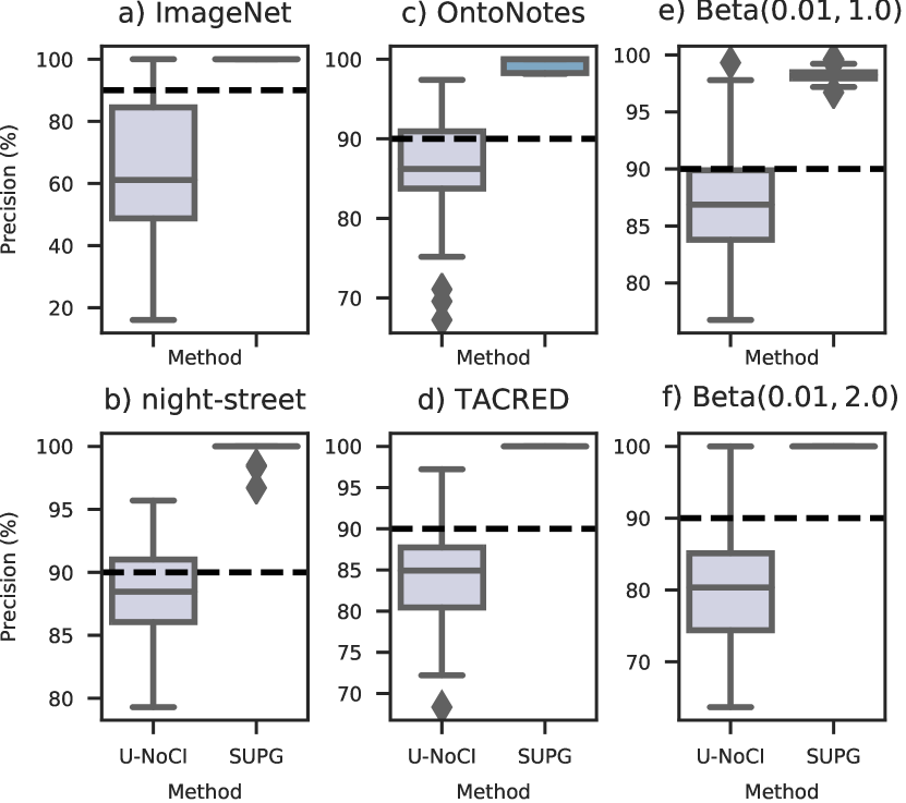
Figure 5: Precision of 100 trials of U-NoCI and SUPG’s importance sampling algorithm with a precision target of 90%. We show a box plot, in which the box 25th, 50th, and 75th quantiles; the minimum and maximum excluding outliers are the “whiskers.” As shown, U-NoCI can fail up to 75% of the time. Furthermore, it can return precisions as low as 20%.

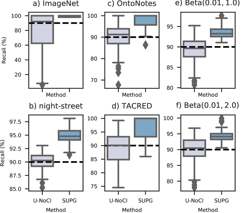
Figure 6: Recall of 100 trials of U-NoCI and SUPG’s importance sampling algorithm with a recall target of 90%. As shown, U-NoCI can fail up to 50% of the time and even catastrophically fail on ImageNet, returning a recall of as low at 20%.

Table 3: Summary of distributionally shifted datasets. These shifts are natural (weather related, different day of video) and synthetic.

Dataset	Shifted dataset	Description
ImageNet	ImageNet-C, Fog	ImageNet with fog
night-street	Day 2	Different days
$\mathrm{Beta}(0.01,1)$	$\mathrm{Beta}(0.01,2)$	Shifted $\beta$ parameter

U-NoCI fails under model drift. We further show that U-NoCI on different data distributions also fails to achieve the failure probability. This procedure is used by existing systems such as NoScope and probabilistic predicates on a given set of data; the cutoff is then used on other data. These systems assume the data distribution is fixed, a known limitation.

To evaluate the effect of model drift, we allow the U-NoCI to choose a proxy threshold using oracle labels on the entire training dataset and then perform selection on test datasets with distributional shift. We compare this with applying the SUPG algorithms using a limited number of oracle labels from the shifted test set as usual. We summarize the shifted datasets in Table 3. We use naturally occurring instances of drift (obscuration by fog [36], different day of video) and synthetic drift (change of $\mathrm{Beta}$ parameters).

As shown in Table 4, baseline methods that do not use labels from the shifted dataset fail to achieve the target in all settings, even under mild conditions such as different days of a video. In fact, using the empirical cutoff in U-NoCI can result in achieved targets as much as 41% lower. In contrast, our algorithms will always respect the failure probability despite model drift, addressing a limitation in prior work [44, 43, 47, 5, 39].

Table 4: Achieved accuracy of queries when using the empirical cutoff method and SUPG on data with distributional shift. We show the average of 100 runs for SUPG. All methods targeted a success rate of 95%. As shown, the naive algorithm deterministically fails to achieve the targets, i.e., has a failure rate of 100%.

	Query		Naive	SUPG
Dataset	type	Target	accuracy	accuracy
ImageNet-C	Precision	95%	77%	100%
ImageNet-C	Recall	95%	54%	100%
night-street	Precision	95%	89%	97%
night-street	Recall	95%	89%	96%
Beta	Precision	95%	89%	100%
Beta	Recall	95%	90%	98%

6.3 SUPG Outperforms Uniform Sampling

We show that SUPG’s novel algorithms for selection outperforms U-CI (i.e., uniform sampling with guarantees) in both the precision target and recall target settings. Recall that the goal is to maximize or minimize the size of the returned set in the precision target and recall target settings, respectively.

Precision target setting. For the datasets and models described in Table 2, we executed U-CI, one-stage importance sampling, and two-stage importance sampling for the precision target setting. We used a budget of 1,000 oracle queries for ImageNet and 10,000 for night-street and the synthetic dataset. We targeted precisions of 0.75, 0.8, 0.9, 0.95, and 0.99.

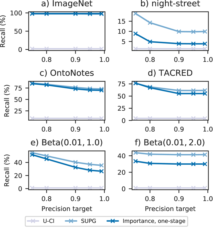
Figure 7: Targeted precision vs achieved recall. As shown, both importance sampling methods outperform U-CI in all cases. Two-stage importance sampling outperforms all methods and matches the one-stage importance sampling for ImageNet.

We show the achieved precision and recall for the various methods in Figure 7. As shown, the importance sampling method outperforms U-CI in all cases. Furthermore, the two-stage algorithm outperforms or matches the one-stage algorithm in all cases except ImageNet. While the specific recalls that are achieved vary per dataset, this is largely due to the performance of the proxy model.

We note that the ImageNet dataset and proxy model are especially favorable to SUPG’s importance sampling algorithms. This dataset has a true positive rate of 0.1% and a highly calibrated proxy. A low true positive rate will result in uniform sampling drawing few positives. In contrast, a highly calibrated proxy will result in many positive draws for importance sampling.

Recall target setting. For the datasets and models in Table 2, we executed U-CI, standard importance sampling with linear weights $\propto A(x)$ (Importance, prop), and the SUPG methods that use sqrt weights. We used the same budgets as in the precision target setting. We targeted recalls of 0.5, 0.6, 0.7, 0.75, 0.8, 0.9, and 0.95.

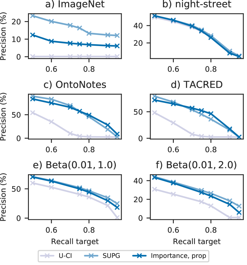
Figure 8: Targeted recall vs precision of the returned set. Up and to the right indicates higher performance. Importance sampling outperforms or matches U-CI in all cases. Our sqrt scaling outperforms proportional scaling for importance sampling in all cases, except for high recall settings.

We show the achieved recall and the returned set size for the various methods in Figure 8. As shown, the importance sampling method outperforms U-CI in all cases. Furthermore, using $\sqrt{A(x)}$ weights outperforms using linear weights in all cases.

6.4 Sensitivity Analysis

We analyze how sensitive our novel algorithms are to: 1) the performance of the proxy model, 2) the class imbalance ratio, and 3) the parameters in our algorithms.

Sensitivity to proxy model. We analyze the sensitivity to the proxy model in two ways: 1) we add noise to the generating distribution for the synthetic dataset and 2) we vary the parameters $\alpha$ and $\beta$ to vary the sharpness of the generating distribution.

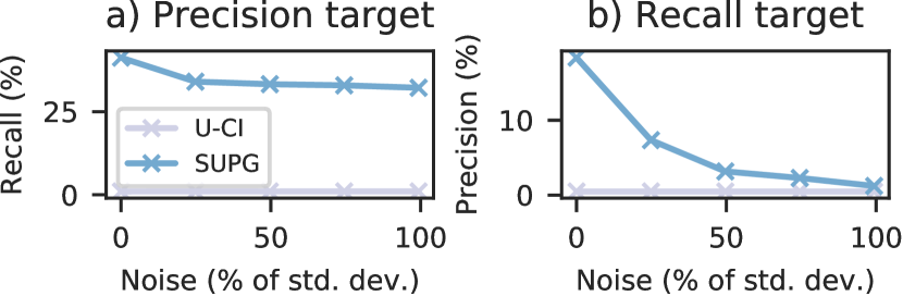
Figure 9: Noise level vs recall/precision for the precision/recall target settings, respectively. The noise level is given as a percent of the standard deviation of the original probabilities. As shown, SUPG outperforms uniform sampling at all noise levels, even up to 100% noise.

First, we generate oracle values from $\mathrm{Beta}(0.01,2)$. After oracle values are generated, we add Gaussian noise to the proxy scores and clip them to $[0,1]$. We add Gaussian noise with standard deviations of 0.01, 0.02, 0.03, and 0.04, which corresponds to 25%, 50%, 75%, and 100% of the standard deviation of the original probabilities. We targeted a precision and recall of 95% and 90% respectively. We show results in Figure 9. As shown, while the performance of our algorithms degrades with higher noise, importance sampling still outperforms uniform sampling at all noise levels. Furthermore, SUPG’s algorithms degrade gracefully with higher noise, especially in the precision target setting.

Second, we vary $\alpha$ and $\beta$ to vary the sharpness. We find that varying $\beta$ as described below (class imbalance) also changes the sharpness of the distribution, as measured by the standard deviation of the probabilities. As the results are the same, we defer the discussion to below. We note that SUPG outperforms uniform sampling in all cases and degrades gracefully as the sharpness of the proxy model decreases.

Sensitivity to class imbalance. We analyze the sensitivity of our algorithms to class imbalance by varying $\alpha$ and $\beta$. We fix $\alpha$ at 0.01 and set $\beta\in\{0.125,0.25,0.5,1.0,2.0\}$.

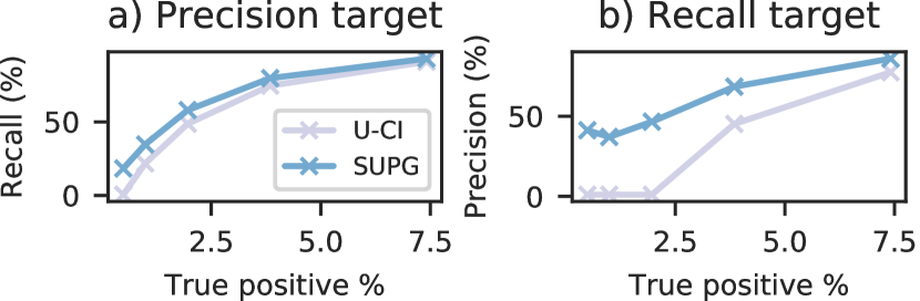
Figure 10: True positive rate vs recall/precision for the precision/recall target settings, respectively. As shown, SUPG outperforms uniform sampling in all scenarios, even as the true positive rate is as high as 7%. SUPG especially outperforms uniform sampling at low true positive rates, outperforming by as much as 47$\times$.

We show results for varying these values in Figure 10. As shown, our algorithms outperform uniform sampling more as the class imbalance is higher. High class imbalance is common in practice, so we optimize our algorithms for such cases. For these cases, SUPG outperforms by as much as 47$\times$. As the data becomes more balanced, our algorithms outperform uniform sampling less, but still outperforms uniform sampling.

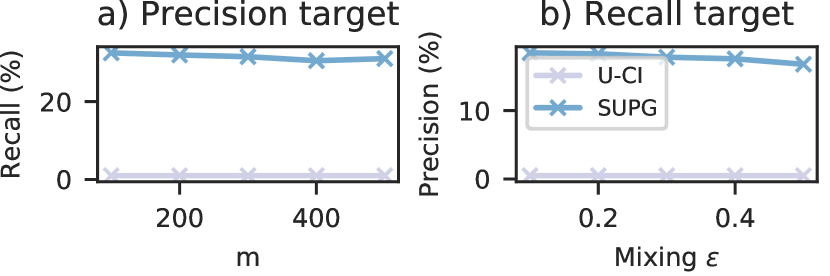
Figure 11: Effect of parameter settings on algorithm performance. As shown, SUPG performs well across a range of parameter settings, indicating that parameters are not difficult to set.

Sensitivity to parameters. We analyze the sensitivity of our algorithms to parameter settings ($m$ in Algorithm 5 and the defensive mixing ratio in Algorithm 4). We vary $m$ from 100 to 500 in increments of 100 and the mixing ratio from 0.1 to 0.5 in increments of 0.1 for $\mathrm{Beta}(0.01,2)$. As shown in Figure 11, SUPG performs well across a range of parameters. We note that some defensive mixing is required to avoid catastrophic failing, but these results indicate that our parameters are not difficult to set by choosing any value away from 0 and 1.

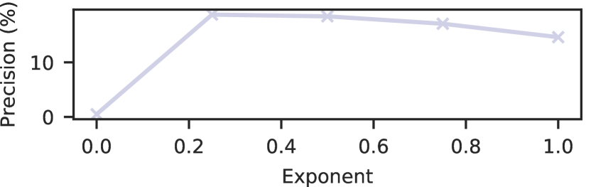
Figure 12: Exponent in importance sampling weights vs precision for the recall target setting. As shown, exponents closer to 0.5 perform better.

Sensitivity to exponent. We analyze the sensitivity to the importance weight exponent by varying it from 0 to 1 for the recall target for $\mathrm{Beta}(0.01,2)$. As shown in Figure 12, exponents corresponding to uniform ($0$) and proportional ($1$) sampling do not perform well. Square root weighting is close to optimal. We note that while our proof shows square root weighting is optimal for estimating counts, optimal end-to-end performance may require slightly different weights. Nonetheless, it outperforms exponents of 0 and 1 and performs well in practice.

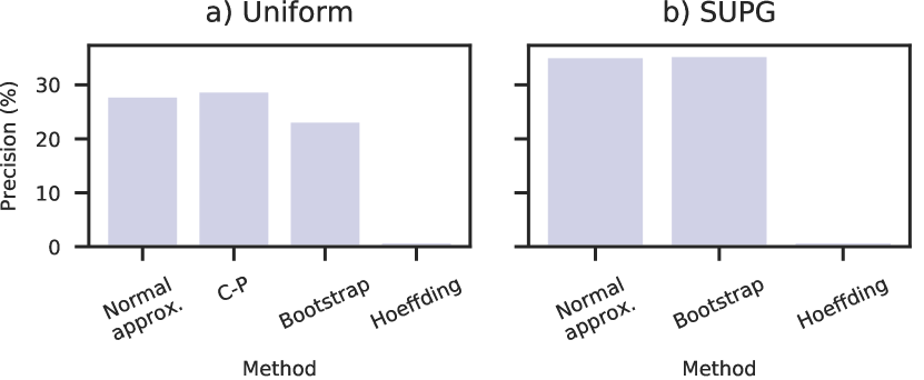
Figure 13: Performance of U-CI-R using various confidence interval methods. As shown, the normal approximation matches or outperforms alternatives, within error margins.

Sensitivity to confidence interval method. We analyze how the confidence interval method affects performance. We consider the normal approximation [9], Hoeffding’s inequality [37], and the bootstrap [24] to compute confidence intervals for both U-CI-R and IS-CI-R. For U-CI-R, we also consider the Clopper-Pearson interval [19]. For all settings, we use $\mathrm{Beta}(0.01,1)$ data with a target recall of 90%. As shown in Figure 13, the normal approximation matches or outperforms other methods within error margins. In particular, Hoeffding’s inequality does not use any property of the data in its confidence interval (e.g., the variance) so it returns vacuous bounds. Since Clopper-Pearson only applies to uniform sampling, we use the normal approximation throughout to standardize confidence interval computation.

Table 5: Cost of SUPG’s query processing, executing the proxy model, executing the oracle predicate, and exhaustive labeling. The oracle are human labelers for all datasets except night, for which the oracle is an expensive DNN (Table 2). As shown, SUPG’s query processing is orders of magnitude cheaper than the other parts of the computation.

	SUPG				Exhaustive
Dataset	Sampling (AWS)	Proxy (AWS)	Oracle	Total	Oracle
night	$$1.7\times 10^{-4}$	$0.02	$2.5	$2.52	$243
ImageNet	$$7.7\times 10^{-5}$	$0.01	$80	$80.01	$4,000
OntoNotes	$$7.7\times 10^{-5}$	$0.02	$80	$80.02	$893
TACRED	$$7.7\times 10^{-5}$	$0.07	$80	$80.07	$1810

6.5 Cost Analysis

We analyze the costs of query processing and executing the proxy/oracle methods. For oracle predicates that are human labels, we approximate the cost by using Scale API’s [1] public costs, at $0.08 per example. We approximate the cost of computation by taking the cost per hour ($3.06) of the Amazon Web Services p3.2xlarge instance. The p3.2xlarge instance contains a single V100 GPU and is commonly used for deep learning.

We show the breakdown of costs in Table 5. As shown, our algorithms are significantly cheaper than exhaustive labeling. Furthermore, the oracle predicate dominates the proxy models. Finally, SUPG query processing costs are negligible compared to the cost of both the proxy and oracle methods.

7 Related Work

Approximate query processing (AQP). AQP aims to return approximate answers to queries for reduced computational complexity [34, 4]. Most AQP systems focus on computing aggregates, such as SUM [14, 50], DISTINCT COUNT [16, 27, 30], and quantiles [2, 21, 26]. Namely, these systems do not aim to answer selection queries. A smaller body of work has studied approximate selection queries [46] with guarantees on precision and recall, though to the best of our knowledge they do not provide probabilistic guarantees or impose hard limits on usage of the predicate oracle, and assume stronger semantics for the proxy.

Optimizing relational predicates. Researchers have proposed numerous methods of reducing the cost of relational queries that contain expensive predicates [35, 17, 33]. To the best of our knowledge, this line of work does not consider approximate selection semantics. In this work, we only consider a single proxy model and a single oracle model, but existing optimization techniques may be useful if multiple oracle models must be applied.

Information retrieval (IR), top-k queries. IR and top-k queries typically aim to rank or select a limited number of data points. Researchers have developed exact [15, 53, 10] and approximate algorithms [7, 12] for these queries. Other algorithms use proxy models for such queries [55, 25]. To the best of our knowledge, these methods and systems do not aim to do exhaustive selection. Furthermore, we introduce notions of statistical guarantees on failure.

Proxy models. Approximate and proxy models have a long history in the machine learning literature, e.g., cascades have been studied in the context of reducing computational costs of classifiers [54, 6, 58]. However, these methods aim to maximize a single metric, such as classification accuracy.

Contemporary visual analytics systems use a specific form of proxy model in the form of specialized neural networks [44, 43, 47, 13, 5, 39]. These specialized neural networks are used to accelerate queries, largely in the form of binary detection [44, 47, 13, 5, 39]. We make use of these models in our algorithms, but the choice and training of the proxy models is orthogonal to our work. Other systems use proxy models to accelerate other query types, such as selection with LIMIT constraints or aggregation queries [43].

8 Discussion and Future Work

While our novel algorithms for approximate selection queries with statistical guarantees show promise, we highlight exciting areas of future work.

First, we have analyzed our algorithms in the asymptotic regime, in which the number of samples goes to infinity. We believe finite-sample complexity bounds will be a fruitful area of future research.

Second, we believe that information-theoretic lower bounds on sample complexity are a fruitful area of future research. If these lower bounds on sample complexity match the upper bounds from the algorithmic analysis, then these algorithms are optimal up to constant factors. As such, we believe these bounds will be helpful in informing future research.

Third, many scenarios naturally can have multiple proxy models. Our algorithms have been developed for single proxy models and show the promise of statistically improved algorithms for approximate selection with guarantees. Furthermore, we believe these algorithms can improve statistical rates relative to single proxy models in certain scenarios.

9 Conclusion

In this work, we develop novel, sample-efficient algorithms to execute approximate selection queries with guarantees. We define query semantics for precision-target and recall-target queries with guarantees on failure probabilities. We implement and evaluate our algorithms, showing that they outperform existing baselines in prior work in all settings we evaluated. These results indicate the promise of probabilistic algorithms to answer selection queries with statistical guarantees. Supporting multiple proxies and even more sample efficient algorithms are avenues for future research.

Acknowledgments

We thank Sahaana Suri, Kexin Rong, and members of the Stanford Infolab for their feedback on early drafts. We further thank Tadashi Fukami, Trevor Hebert, and Isaac Westlund for their helpful discussions. The hummingbird data was collected by Kaoru Tsuji, Trevor Hebert, and Tadashi Fukami, funded by a Kyoto University Foundation grant and an NSF Dimensions of Biodiversity grant (DEB-1737758). This research was supported in part by affiliate members and other supporters of the Stanford DAWN project—Ant Financial, Facebook, Google, Infosys, NEC, and VMware—as well as Toyota Research Institute, Northrop Grumman, Amazon Web Services, Cisco, and the NSF under CAREER grant CNS-1651570. Any opinions, findings, and conclusions or recommendations expressed in this material are those of the authors and do not necessarily reflect the views of the NSF. Toyota Research Institute ("TRI") provided funds to assist the authors with their research but this article solely reflects the opinions and conclusions of its authors and not TRI or any other Toyota entity.

10 Additional Proofs

10.1 Theorem 1

Proof.

We decompose the variance conditioned on $a(x)$:

$$V\coloneqq \mathop{\text{Var}}_{x\sim w}[f(x)u(x)/w(x)]$$

$$= \mathop{\mathbb{E}}_{x\sim w}\left[\mathop{\text{Var}}_{x\sim w}[f(x)\frac{u(x)}{w(x)}|a(x)]\right]+$$

$$\mathop{\text{Var}}_{x\sim w}\left[\mathop{\mathbb{E}}_{x\sim w}[f(x)\frac{u(x)}{w(x)}|a(x)]\right].$$

Since $u(x),w(x)$ are known given $a(x)$ but $f(x)$ is not,

$$V =\mathop{\mathbb{E}}_{x\sim w}\left[a(x)(1-a(x))\frac{u(x)^{2}}{w(x)^{2}}\right]+\mathop{\text{Var}}_{x\sim w}\left[a(x)\frac{u(x)}{w(x)}\right]$$

$$=\mathop{\mathbb{E}}_{x\sim w}\left[a(x)\frac{u(x)^{2}}{w(x)^{2}}\right]-\mathop{\mathbb{E}}_{x\sim w}\left[a(x)\frac{u(x)}{w(x)}\right]^{2}$$

$$=\sum_{x}\left[a(x)\frac{u(x)^{2}}{w(x)}\right]-\mathop{\mathbb{E}}_{x\sim u}\left[a(x)\right]^{2}$$

In order to solve for the $w(x)$ minimizing $V$, we introduce the Lagrangian dual for the constraint $\sum_{x}w(x)=1$ and then take partial derivatives of

$$L\coloneqq\sum_{x}\left[a(x)\frac{u(x)^{2}}{w(x)}\right]-\mathop{\mathbb{E}}_{x\sim u}\left[a(x)\right]^{2}-\lambda\left(\sum_{x}w(x)-1\right)$$

w.r.t. $w(x)$ to find that $-w(x)^{-2}a(x)u(x)^{2}=\lambda$, so $w(x)=C\sqrt{a(x)}u(x)$ for a normalizing constant $C$. ∎

10.2 Variance comparisons

Let $V_{1}\coloneqq\sum_{x}\left[a(x)\frac{u(x)^{2}}{w(x)}\right]$ so that $V=V_{1}-E_{u}[a(x)]^{2}$. In this derivation we assume a uniform distribution $u(x)$. For uniform $w(x)$, we have that

$$V_{1}^{(u)}=\sum_{x}a(x)u(x)=\mathop{\mathbb{E}}_{x\sim u}[a(x)]$$

For $w(x)\propto a(x)$:

$$V_{1}^{(p)} =\frac{1}{n^{2}}\sum_{\{x:a(x)>0\}}a(x)\cdot\frac{\sum_{x^{\prime}}a(x^{\prime})}{a(x)}$$

$$=\Pr(a(x)>0)\mathop{\mathbb{E}}_{x\sim u}[a(x)]$$

For $w(x)\propto\sqrt{a(x)}$:

$$V_{1}^{(s)}=\frac{1}{n^{2}}\sum_{x}a(x)\cdot\frac{\sum_{x^{\prime}}\sqrt{a(x^{\prime})}}{\sqrt{a(x)}}=\mathop{\mathbb{E}}_{x\sim u}[\sqrt{a(x)}]^{2}$$

We now show that these variances satisfy $V_{1}^{(s)}\leq V_{1}^{(p)}\leq V_{1}^{(u)}$.

First, note that $\Pr(a(x)>0)\leq 1$ implies $V_{1}^{(p)}\leq V_{1}^{(u)}$.

Using Hölder’s inequality, we have that

$$\mathop{\mathbb{E}}_{x\sim u}[\sqrt{a(x)}1_{a(x)>0}]\leq\mathop{\mathbb{E}}_{x\sim u}[a(x)]^{1/2}\mathop{\mathbb{E}}_{x\sim u}[1_{a(x)>0}]^{1/2}.$$

Squaring both sides yields

$$\mathop{\mathbb{E}}_{x\sim u}[\sqrt{a(x)}]^{2}\leq\mathop{\mathbb{E}}_{x\sim u}[a(x)]\Pr(a(x)>0).$$

Finally, note that the gap between the optimal and uniform weights has a simple form

$$V_{1}^{(u)}-V_{1}^{(s)}=\mathop{\text{Var}}_{x\sim u}[\sqrt{a(x)}].$$

Appendix A Queries with Both a Precision and Recall Target

Certain applications may require both precision and recall targets simultaneously. We refer to queries that impose both targets as JT queries. Unlike with PT and RT queries, achieving these targets may not be possible given a maximum oracle label budget. In our experience, industry and research applications usually prefer queries that can operate under a budget so JT queries are less practical. Nonetheless, we discuss syntax and semantics of such queries, describe algorithms that provide guarantees, and evaluate these algorithms.

⬇

SELECT * FROM table_name

WHERE filter_predicate

USING proxy_estimates

RECALL TARGET tr

PRECISION TARGET tp

WITH PROBABILITY p

Figure 14: Syntax for specifying approximate selection queries with both a precision and recall target. Users provide both a precision and recall target in addition to a probability of success. Such queries do not have an oracle budget, as the oracle may be queried an unbounded number of times.

Syntax and semantics. We define the syntax for queries with both a recall and precision target in Figure 14. Such queries do not specify an oracle budget and instead specify both a precision and recall target. All other syntax elements are a direct extension of the syntax for PT and RT queries in Figure 3.

The semantics of such queries remains similar, except the recall and precision targets must be jointly satisfied with a failure probability.

Algorithms. We describe how the recall target algorithms can be used as a subroutine for the joint target (JT) setting. We note a modified version of the precision target algorithm can be used as a subroutine instead, but defer the analysis and evaluation to future work.

The joint algorithm proceeds in three stages.

1. Optimistically allocate a budget $B$.

2. Run an RT algorithm (IS-CI-R) with budget $B$ to achieve the recall target $\gamma_{r}$.

3. Exhaustively filter out false positives from stage two using oracle queries.

This algorithm achieves the recall target because the RT algorithm will return a set of records with sufficient positive matches with high probability. Then, since we exhaustively query the oracle on the results from stage two in the third stage, we can prune the results to achieve a precision target while maintaining the recall. Note that the third stage is necessary because even with a large budget for estimating a proxy score threshold $\gamma_{r}$, there may not exist any threshold that would allow us to directly identify a set of records with high enough precision and recall. The proxy may simply be too weak to identify records with the required precision and recall targets, so any JT algorithm will have to supplement sets of records identified by the proxy with additional processing.

Evaluation. We evaluate the joint algorithm when using uniform sampling and our improved importance sampling recall target algorithms as subroutines. For comparison, we use the same budget as our evaluations in Section 6.3 to run stage 2 of the JT method.

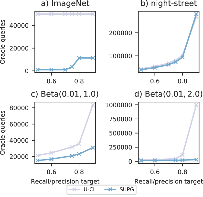
Figure 15: SUPG and uniform sampling on joint target queries. As shown, SUPG generally outperforms uniform sampling.

We target precision/recall targets of 0.5, 0.6, 0.7, 0.75, 0.8, and 0.9 and executed the joint algorithms. We show the recall/precision target vs the number of oracle queries in Figure 15. As shown, SUPG generally outperforms uniform sampling.

References

- [1] Scale API: The API for training data, 2020.
- [2] P. K. Agarwal, G. Cormode, Z. Huang, J. M. Phillips, Z. Wei, and K. Yi. Mergeable summaries. ACM Transactions on Database Systems (TODS), 38(4):1–28, 2013.
- [3] S. Agarwal, H. Milner, A. Kleiner, A. Talwalkar, M. Jordan, S. Madden, B. Mozafari, and I. Stoica. Knowing when you’re wrong: building fast and reliable approximate query processing systems. In SIGMOD, pages 481–492. ACM, 2014.
- [4] S. Agarwal, B. Mozafari, A. Panda, H. Milner, S. Madden, and I. Stoica. Blinkdb: queries with bounded errors and bounded response times on very large data. In EuroSys, pages 29–42. ACM, 2013.
- [5] M. R. Anderson, M. Cafarella, T. F. Wenisch, and G. Ros. Predicate optimization for a visual analytics database. ICDE, 2019.
- [6] A. Angelova, A. Krizhevsky, V. Vanhoucke, A. Ogale, and D. Ferguson. Real-time pedestrian detection with deep network cascades. 2015.
- [7] V. N. Anh, O. de Kretser, and A. Moffat. Vector-space ranking with effective early termination. In Proceedings of the 24th annual international ACM SIGIR conference on Research and development in information retrieval, pages 35–42, 2001.
- [8] S. Beery, D. Morris, and S. Yang. Efficient pipeline for camera trap image review. arXiv preprint arXiv:1907.06772, 2019.
- [9] V. Bentkus and F. Gotze. The Berry-Esseen bound for Student’s statistic. The Annals of Probability, 24(1):491–503, 1996.
- [10] A. Z. Broder, D. Carmel, M. Herscovici, A. Soffer, and J. Zien. Efficient query evaluation using a two-level retrieval process. In Proceedings of the twelfth international conference on Information and knowledge management, pages 426–434, 2003.
- [11] M. Buckland and F. Gey. The relationship between recall and precision. Journal of the American society for information science, 45(1):12–19, 1994.
- [12] B. B. Cambazoglu, H. Zaragoza, O. Chapelle, J. Chen, C. Liao, Z. Zheng, and J. Degenhardt. Early exit optimizations for additive machine learned ranking systems. In Proceedings of the third ACM international conference on Web search and data mining, pages 411–420, 2010.
- [13] C. Canel, T. Kim, G. Zhou, C. Li, H. Lim, D. Andersen, M. Kaminsky, and S. Dulloor. Scaling video analytics on constrained edge nodes. SysML, 2019.
- [14] K. Chakrabarti, M. Garofalakis, R. Rastogi, and K. Shim. Approximate query processing using wavelets. The VLDB Journal, 10(2-3):199–223, 2001.
- [15] K. C.-C. Chang and S.-w. Hwang. Minimal probing: supporting expensive predicates for top-k queries. In SIGMOD, pages 346–357, 2002.
- [16] M. Charikar, S. Chaudhuri, R. Motwani, and V. Narasayya. Towards estimation error guarantees for distinct values. In Proceedings of the nineteenth ACM SIGMOD-SIGACT-SIGART symposium on Principles of database systems, pages 268–279, 2000.
- [17] S. Chaudhuri and K. Shim. Optimization of queries with user-defined predicates. ACM Transactions on Database Systems (TODS), 24(2):177–228, 1999.
- [18] E. Choi, O. Levy, Y. Choi, and L. Zettlemoyer. Ultra-fine entity typing. ACL, 2018.
- [19] C. J. Clopper and E. S. Pearson. The use of confidence or fiducial limits illustrated in the case of the binomial. Biometrika, 26(4):404–413, 1934.
- [20] T. H. Cormen, C. E. Leiserson, R. L. Rivest, and C. Stein. Introduction to algorithms. MIT press, 2009.
- [21] G. Cormode and S. Muthukrishnan. An improved data stream summary: the count-min sketch and its applications. Journal of Algorithms, 55(1):58–75, 2005.
- [22] J. Devlin, M.-W. Chang, K. Lee, and K. Toutanova. Bert: Pre-training of deep bidirectional transformers for language understanding. arXiv preprint arXiv:1810.04805, 2018.
- [23] B. Dwyer. A popular self-driving car dataset is missing labels for hundreds of pedestrians. https://blog.roboflow.ai/self-driving-car-dataset-missing-pedestrians/, 2020.
- [24] B. Efron. Bootstrap methods: another look at the jackknife. In Breakthroughs in statistics, pages 569–593. Springer, 1992.
- [25] L. Gallagher, R.-C. Chen, R. Blanco, and J. S. Culpepper. Joint optimization of cascade ranking models. In Proceedings of the Twelfth ACM International Conference on Web Search and Data Mining, pages 15–23, 2019.
- [26] E. Gan, J. Ding, K. S. Tai, V. Sharan, and P. Bailis. Moment-based quantile sketches for efficient high cardinality aggregation queries. PVLDB, 11(11):1647–1660, 2018.
- [27] P. B. Gibbons. Distinct sampling for highly-accurate answers to distinct values queries and event reports. In VLDB, volume 1, pages 541–550, 2001.
- [28] M. Gordon and M. Kochen. Recall-precision trade-off: A derivation. Journal of the American Society for Information Science, 40(3):145–151, 1989.
- [29] P. J. Haas and J. M. Hellerstein. Ripple joins for online aggregation. ACM SIGMOD Record, 28(2):287–298, 1999.
- [30] P. J. Haas, J. F. Naughton, S. Seshadri, and L. Stokes. Sampling-based estimation of the number of distinct values of an attribute. In VLDB, volume 95, pages 311–322, 1995.
- [31] K. He, G. Gkioxari, P. Dollár, and R. Girshick. Mask r-cnn. In ICCV, pages 2980–2988. IEEE, 2017.
- [32] K. He, X. Zhang, S. Ren, and J. Sun. Deep residual learning for image recognition. In CVPR, pages 770–778, 2016.
- [33] J. M. Hellerstein. Optimization techniques for queries with expensive methods. ACM Transactions on Database Systems (TODS), 23(2):113–157, 1998.
- [34] J. M. Hellerstein, P. J. Haas, and H. J. Wang. Online aggregation. In Acm Sigmod Record, volume 26, pages 171–182. ACM, 1997.
- [35] J. M. Hellerstein and M. Stonebraker. Predicate migration: Optimizing queries with expensive predicates. In SIGMOD, pages 267–276, 1993.
- [36] D. Hendrycks and T. G. Dietterich. Benchmarking neural network robustness to common corruptions and surface variations. arXiv preprint arXiv:1807.01697, 2018.
- [37] W. Hoeffding. Probability inequalities for sums of bounded random variables. In The Collected Works of Wassily Hoeffding, pages 409–426. Springer, 1994.
- [38] E. Hovy, M. Marcus, M. Palmer, L. Ramshaw, and R. Weischedel. Ontonotes: the 90% solution. In NAACL, pages 57–60, 2006.
- [39] K. Hsieh, G. Ananthanarayanan, P. Bodik, P. Bahl, M. Philipose, P. B. Gibbons, and O. Mutlu. Focus: Querying large video datasets with low latency and low cost. OSDI, 2018.
- [40] E. Inc. Artificial intelligence driven e-discovery - exterro. https://www.exterro.com/ai/, 2020.
- [41] T. Inc. Text iq: Ai solutions for law firms and inside counsel. https://www.textiq.com/legal, 2020.
- [42] M. Joshi, D. Chen, Y. Liu, D. S. Weld, L. Zettlemoyer, and O. Levy. Spanbert: Improving pre-training by representing and predicting spans. Transactions of the Association for Computational Linguistics, 8:64–77, 2020.
- [43] D. Kang, P. Bailis, and M. Zaharia. Blazeit: Optimizing declarative aggregation and limit queries for neural network-based video analytics. PVLDB, 13(4):533–546, 2019.
- [44] D. Kang, J. Emmons, F. Abuzaid, P. Bailis, and M. Zaharia. Noscope: optimizing neural network queries over video at scale. PVLDB, 10(11):1586–1597, 2017.
- [45] D. Kang, E. Gan, P. Bailis, T. Hashimoto, and M. Zaharia. Approximate selection with guarantees using proxies. arXiv preprint arXiv:2004.00827, 2020.
- [46] I. Lazaridis and S. Mehrotra. Approximate selection queries over imprecise data. In Proceedings. 20th International Conference on Data Engineering, pages 140–151, April 2004.
- [47] Y. Lu, A. Chowdhery, S. Kandula, and S. Chaudhuri. Accelerating machine learning inference with probabilistic predicates. In SIGMOD, pages 1493–1508. ACM, 2018.
- [48] C. D. Manning, P. Raghavan, and H. Schütze. Introduction to Information Retrieval. Cambridge University Press, USA, 2008.
- [49] A. Owen and Y. Zhou. Safe and effective importance sampling. Journal of the American Statistical Association, 95(449):135–143, 2000.
- [50] V. Poosala and V. Ganti. Fast approximate answers to aggregate queries on a data cube. In Proceedings. Eleventh International Conference on Scientific and Statistical Database Management, pages 24–33. IEEE, 1999.
- [51] O. Russakovsky, J. Deng, H. Su, J. Krause, S. Satheesh, S. Ma, Z. Huang, A. Karpathy, A. Khosla, M. Bernstein, et al. Imagenet large scale visual recognition challenge. International journal of computer vision, 115(3):211–252, 2015.
- [52] P. A. San Juan, J. N. Hendershot, G. C. Daily, and T. Fukami. Land-use change has host-specific influences on avian gut microbiomes. The ISME Journal, 14(1):318–321, 2020.
- [53] H. Turtle and J. Flood. Query evaluation: strategies and optimizations. Information Processing & Management, 31(6):831–850, 1995.
- [54] P. Viola and M. Jones. Rapid object detection using a boosted cascade of simple features. In Proceedings of the 2001 IEEE computer society conference on computer vision and pattern recognition. CVPR 2001, volume 1, pages I–I. IEEE, 2001.
- [55] L. Wang, J. Lin, and D. Metzler. A cascade ranking model for efficient ranked retrieval. In Proceedings of the 34th international ACM SIGIR conference on Research and development in Information Retrieval, pages 105–114, 2011.
- [56] L. Wasserman. All of statistics: a concise course in statistical inference. Springer Science & Business Media, 2013.
- [57] T. Xu, L. M. Botelho, and F. X. Lin. Vstore: A data store for analytics on large videos. In Proceedings of the Fourteenth EuroSys Conference 2019, page 16. ACM, 2019.
- [58] F. Yang, W. Choi, and Y. Lin. Exploit all the layers: Fast and accurate cnn object detector with scale dependent pooling and cascaded rejection classifiers. In Proceedings of the IEEE conference on computer vision and pattern recognition, pages 2129–2137, 2016.
- [59] Y. Zhang, V. Zhong, D. Chen, G. Angeli, and C. D. Manning. Position-aware attention and supervised data improve slot filling. In Proceedings of the 2017 Conference on Empirical Methods in Natural Language Processing (EMNLP 2017), pages 35–45, 2017.