Quantifying the effect of field variance on the H$\alpha$ luminosity function with the New Numerical Galaxy Catalogue ($\nu^{2}$GC)

Abstract

We construct a model of H$\alpha$ emitters (HAEs) based on a semi-analytic galaxy formation model, the New Numerical Galaxy Catalog ($\nu^{2}$GC). In this paper, we report our estimate for the field variance of the HAE distribution. By calculating the H$\alpha$ luminosity from the star-formation rate of galaxies, our model well reproduces the observed H$\alpha$ luminosity function (LF) at $z=0.4$. The large volume of the $\nu^{2}$GC makes it possible to examine the spatial distribution of HAEs over a region of (411.8 Mpc)³ in the comoving scale. The surface number density of $z=0.4$ HAEs with $L_{\rm H\alpha}\geq 10^{40}$ erg s^-1 is 308.9 deg^-2. We have confirmed that the HAE is a useful tracer for the large-scale structure of the Universe because of their significant overdensity ($>5\sigma$) at clusters and the filamentary structures. The H$\alpha$ LFs within a survey area of $\sim$2 deg² (typical for previous observational studies) show a significant field variance up to $\sim$1 dex. Based on our model, one can estimate the variance on the H$\alpha$ LFs within given survey areas.

1 Introduction

So far, various extensive observations of star-forming galaxies have shown that galaxies do not distribute uniformly and that their spatial distribution shows various structures at various spatial scales (e.g., de Lapparent et al., 1986; Ho et al., 2012; Ross et al., 2012). The formation of such a large-scale structure (LSS) of the Universe has been investigated by $N$-body simulations. Structure formation is powered by gravitational instabilities of cold dark matter (CDM) and form dark matter halos where galaxies form and evolve (e.g., Springel et al., 2005).

For investigating the evolution of the galaxies and structure formation, emission-line galaxies (ELGs) have been often used (e.g., Shimasaku et al., 2003; Ouchi et al., 2003; Hayashino et al., 2004; Matsuda et al., 2004; Ouchi et al., 2008; Geach et al., 2008; Hayashi et al., 2010; Mawatari et al., 2012; Kodama et al., 2013; Darvish et al., 2014; Khostovan et al., 2015; Shimakawa et al., 2017; Ogura et al., 2017; Ouchi et al., 2018; Shibuya et al., 2018) because emission lines from galaxies, such as [O ii] ($\lambda\lambda$3727, 3730), [O iii] ($\lambda\lambda$4959, 5007), and H$\alpha$ ($\lambda$6563), are good indicators for the star-formation rate (SFR) of galaxies (e.g., Kennicutt, 1998; Kewley et al., 2004; Moustakas et al., 2006; Hayashi et al., 2013; Suzuki et al., 2016). A strong point to focus on ELGs is that we can observe them over a significantly wide area by utilizing the combination of narrow-band (NB) filters and wide-field cameras. Note that, although spectroscopic surveys including the integral field spectroscopy are more powerful than NB surveys to identify emission lines and to measure accurate line luminosities, the survey area with enough depth is limited. Therefore, it is difficult to trace the LSS by spectroscopic observations, except for some samples in the bright regime (e.g., Durkalec et al., 2015).

Among such ELGs, H$\alpha$ emitters (HAEs) are often focused since H$\alpha$ emission is well calibrated and only mildly affected by the dust attenuation compared to other emission lines at wavelengths bluer than H$\alpha$ (e.g., Garn et al., 2010; Garn, & Best, 2010; Stott et al., 2013; Sobral et al., 2015). Moreover, the H$\alpha$ emission line from galaxies at a wide redshift range ($0\leq z\lesssim 2.6$) can be observed with NB imaging using ground-based optical and NIR instruments. So far, many surveys using NB filters have been conducted to make a large sample of HAEs over a wide redshift range (e.g., Kodama et al., 2004; Ly et al., 2007, 2011; Matsuda et al., 2011; Hatch et al., 2011; Tanaka et al., 2011; Koyama et al., 2011, 2013; Sobral et al., 2011, 2013, 2015; Drake et al., 2013; Matthee et al., 2017; Stroe et al., 2017; Hayashi et al., 2018).

The field variance (or “cosmic variance”) has been recognized as a serious problem in observational studies of high-$z$ galaxies (Somerville et al., 2004; Trenti & Stiavelli, 2008). It is the uncertainty in measuring the number density of galaxies due to underlying density fluctuation of dark matter. Indeed, while luminosity functions (LFs) of ELGs obtained by some different surveys generally show good agreement, some of them are in some disagreement by a factor of a few (e.g., Ly et al., 2011; Lee et al., 2012; Sobral et al., 2012; Colbert et al., 2013; Stroe et al., 2014). Because most of previous surveys covered less than 2 deg² area, the results could be caused by the field variance. To reduce the effect of the field variance, Sobral et al. (2015) performed $\sim$10 deg² survey while the survey depth is somewhat shallow. Very recently, Hayashi et al. (2018) construct the largest sample of ELGs so far by utilizing deep and wide data in a $\sim$16 deg² area provided by the first public data release (Aihara et al., 2018b) of the Subaru Strategic Survey with Hyper Suprime-Cam (Miyazaki et al., 2012) on the Subaru telescope (HSC-SSP; Aihara et al., 2018a). The H$\alpha$ LF at $z=0.4$ derived by Hayashi et al. (2018) shows a good agreement with previous surveys reported by Ly et al. (2007), Drake et al. (2013) and Sobral et al. (2013). However, all of these studies employ different threshold of equivalent width (EW) for selecting HAEs; specifically, the rest-frame equivalent width ($EW_{0}$) $\geq 40$ Å (Hayashi et al., 2018), $EW_{0}\geq 11$ Å (Ly et al., 2007), $EW_{0}\geq 100$ Å (Drake et al., 2013), and $EW_{0}\geq 25$ Å (Sobral et al., 2013). Furthermore, Hayashi et al. (2018) show that H$\alpha$ LFs obtained in different fields show significant variance up to $\sim$1 dex. How large is the field variance in a given survey area ? How wide is survey area required to converge the LF ? These are still open questions.

To tackle this issue, we examine the field variance of the spatial distribution of galaxies by using a semi-analytic galaxy formation model, the New Numerical Galaxy Catalog ($\nu^{2}$GC; Makiya et al., 2016; Shirakata et al., 2019). A remarkable aspect of the $\nu^{2}$GC is a large comoving volume up to $\sim$4.5 Gpc³ with sufficient mass resolution based on the state-of-the-art cosmological $N$-body simulations by Ishiyama et al. (2015). This enables us to examine various statistical properties of galaxies over a wide area. Indeed, the $\nu^{2}$GC is successful to reproduce observed statistical properties of galaxies in a wide redshift range of $0\leq z<6$ such as the Hi mass function, broad-band LF, and cosmic star-formation history (see Makiya et al., 2016; Shirakata et al., 2019, for more details). By utilizing the $\nu^{2}$GC, we construct a model of HAEs to examine the field variance of their spatial distribution. In this paper, we focus on HAEs at $z=0.4$ at which extensive observations of HAEs has been conducted (Ly et al., 2007; Drake et al., 2013; Sobral et al., 2013; Hayashi et al., 2018).

This paper is organized as follows. We present overview of the $\nu^{2}$GC and the HAE model in Section 2. The properties of model HAEs including the H$\alpha$ LF are described in Section 3. In Section 4, we discuss the field variance on the H$\alpha$ LF. We then give our conclusion in Section 5. Throughout this paper, we employ a $\Lambda$CDM cosmology in which $h_{0}=0.68$, $\Omega_{\rm M}=0.31$, and $\Omega_{\rm\Lambda}=0.69$ (Planck Collaboration et al., 2014), unless otherwise stated. Given these parameters, 1 arcsec corresponds to 5.515 physical kpc at $z=0.4$. We adopt the Chabrier initial mass function (IMF) in the mass range of 0.1 – 100 $M_{\odot}$ (Chabrier, 2003). All magnitudes are given in the AB system (Oke & Gunn, 1983).

2 Model

2.1 The $\nu^{2}$GC

The $\nu^{2}$GC (Makiya et al., 2016; Shirakata et al., 2019) is a semi-analytic model for the galaxy formation, which is an updated version of the Numerical Galaxy Catalog ($\nu$GC; Nagashima et al., 2005; Enoki et al., 2014; Shirakata et al., 2015). We use the $\nu^{2}$GC-S (Ishiyama et al., 2015), which is an $N$-body simulation with a box of (280 $h^{-1}$ Mpc)³ comoving scale [corresponding to (411.8 Mpc)³ when we adopt $h_{0}=0.68$] containing 2048³ dark matter particles, for constructing merger trees of dark matter halos. The particle mass resolution, the minimum halo mass and the total number of halos in the box are 2.20$\times 10^{8}$ $M_{\odot}$, 8.79$\times 10^{9}$ $M_{\odot}$ and 6,575,486, respectively. The large comoving volume of this simulation enables us to examine the statistical properties of galaxies including the spatial distribution over a wide area. Note that 411.8 Mpc in the comoving scale at $z=0.4$ corresponds to 14.8 degree on the sky.

The $\nu^{2}$GC includes many physical processes involved in the galaxy formation and evolution. We briefly summarize here the baryonic evolution model in the $\nu^{2}$GC. See Makiya et al. (2016) and Shirakata et al. (2019) for further details of the model. We assume that a dark matter halo is filled with the hot gas with the virial temperature. The hot gas cools through the radiation cooling to form a gas disk. Here, we employ a scheme of the gas cooling rate proposed by White & Frenk (1991) and a cooling function provided by Sutherland & Dopita (1993). The cold gas in the disk condenses to form stars. The star-formation rate (SFR) is given by

$$SFR=M_{\rm cold}/\tau_{\rm star},$$ (1)

where $M_{\rm cold}$ and $\tau_{\rm star}$ are the cold gas mass and the star-formation timescale, respectively. By assuming that the star-formation in the galactic disk is related to the dynamical time scale of the disk, $\tau_{\rm d}$ ($\equiv r_{\rm d}/V_{\rm d}$, where $r_{\rm d}$ and $V_{\rm d}$ are the radius of the disk and the disk rotation velocity, respectively), the star-formation timescale is given by the following formula:

$$\tau_{\rm star}=\varepsilon_{\rm star}^{-1}\tau_{\rm d}\left[1+\Bigl{(}\frac{V_{\rm d}}{V_{\rm hot}}\Bigr{)}^{\alpha_{\rm star}}\right],$$ (2)

where $\alpha_{\rm star}$, $\varepsilon_{\rm star}$, and $V_{\rm hot}$ are free parameters that are determined by fitting observed LFs ($r$- and $K$-bands) and cold neutral gas mass function at $z=0$ based on a Markov chain Monte Carlo (MCMC) method. The best fit values of these parameters are $\alpha_{\rm star}=-2.14$, $\varepsilon_{\rm star}=0.48$, and $V_{\rm hot}=121.64$ km s^-1 (see Makiya et al., 2016; Shirakata et al., 2019, for the detail of the parameter tuning).

As for the feedback, we assume that Type-II supernovae reheat a part of the cold gas to reject it from the galaxies at a rate of $M_{\rm cold}/\tau_{\rm reheat}$ (the effects of the type-Ia supernovae are negrected). The reheating timescale $\tau_{\rm reheat}$ is given by following equation:

$$\tau_{\rm reheat}=\frac{\tau_{\rm star}}{\beta(V_{\rm d})},$$ (3)

where

$$\beta(V_{\rm d})\equiv\Bigl{(}\frac{V_{\rm d}}{V_{\rm hot}}\Bigr{)}^{-\alpha_{\rm hot}},$$ (4)

with free parameters of $V_{\rm hot}$ [the same as $V_{\rm hot}$ in equation (2), with a best fit value of 121.64 km s^-1] and $\alpha_{\rm hot}$ (the best fit value is $\alpha_{\rm hot}$ = 3.92) is the reheating timescale.

When two or more galaxies merge together, we assume that a starburst occurs and consume the cold gas in the bulge. The mass of stars formed by a starburst, $\Delta M_{\rm star,burst}$, is given by

$$\Delta M_{\rm star,burst}=\frac{\alpha}{\alpha+\beta+f_{\rm BH}}M^{0}_{\rm cold},$$ (5)

where $M^{0}_{\rm cold}$ is the cold gas mass right after the burst, $\alpha$ is the locked-up mass fraction, $\beta$ is defined by the equation (4), and $f_{\rm BH}$ is the fraction of the gas which is accreted onto the supermassive black hole (SMBH). The locked-up mass fraction $\alpha$ is set to be consistent with IMF ($\alpha=0.52$ for the Chabrier IMF). We set $f_{\rm BH}$ to reproduce observed relation between host bulge mass and SMBH mass ($f_{\rm BH}=0.02$, see Shirakata et al., 2019). Note that even in the case of the minor merger, a starburst occurs.

Based on these processes, the star-formation history and metal-enrichment history of each galaxy are computed. We calculate the spectral energy distribution by synthesizing a simple stellar population model provided by Bruzual & Charlot (2003). We calculate the dust extinction by assuming (1) the dust-to-gas ratio is proportional to the cold gas metallicity, (2) the optical depth of the dust is proportional to the column density of the dust, (3) the dust geometry follows the slab dust model (Disney et al., 1989), and (4) the wavelength dependence of the attenuation obeys the Calzetti law (Calzetti et al., 2000). Our model also includes the evolution of the SMBHs and properties of active galactic nuclei (AGNs). See Shirakata et al. (2019) for details of the latest model of the SMBH growth and AGN properties.

2.2 H$\alpha$ luminosity

We make a mock catalog of galaxies at $z=0.4$ in a (411.8 Mpc)³ box based on the $\nu^{2}$ GC. The mock catalog includes 3,100,052 galaxies brighter than –15 mag in SDSS $r$-band. We calculate intrinsic luminosity of H$\alpha$ emission from each galaxy simply by converting from the SFR adopting the Kennicutt (1998) relation corrected for the Chabrier IMF:

$$L_{{\rm H}\alpha}^{\rm int}~{}[{\rm erg~{}s}^{-1}]=SFR~{}[M_{\odot}~{}{\rm yr}^{-1}]/(4.4\times 10^{-42}).$$ (6)

Here we use the mean SFRs during dynamical times of disks and bulges for normal star-forming galaxies and starburst galaxies, respectively.

The dust attenuation level of the nebular emission line compared to that of the continuum emission, $f_{\rm neb}$, is often quantified by the following expression:

$$f_{\rm neb}\equiv E(B-V)_{\rm star}/E(B-V)_{\rm line}$$ (7)

(e.g., Koyama et al., 2019). Various observational studies report that $f_{\rm neb}=0.44-0.6$ at $z<1$ (Calzetti et al., 2000; Wuyts et al., 2011; Pannella et al., 2015). In this study, we employ a fixed value of $f_{\rm neb}=0.5$. Including the dust extinction, the observable luminosity of H$\alpha$ emission, $L_{{\rm H}\alpha}^{\rm obs}$, is calculated. Here we note that some previous observational studies at higher redshift ($z>0.8$) showed that AGN-powered HAEs could contribute to the luminous HAE sample (e.g., Sobral et al., 2016; Matthee et al., 2017). According to Sobral et al. (2016), the number fraction of AGNs in luminous HAEs at $z=0.8-2.2$ is $\sim$30%. They also found that the AGN fraction increases with $L_{\rm H\alpha}$ at $L_{\rm H\alpha}\geq 10^{42}$ erg s^-1. This trend is constant independent of the redshifts (at least at $z=0.8-2.3$). Although, at high redshifts, the mechanism of AGN that enhances the Ha luminosity may play an important role on the H$\alpha$ LF at the bright end, at $z\sim 0.4$, the HAEs at $L_{\rm H\alpha}\geq 10^{42}$ erg s^-1 are relatively rare (e.g., Schulze et al., 2009; Hayashi et al., 2018).

Since we here focus on the field variance of the LFs of HAEs much fainter than the bright end, we do not include the contribution from the HAEs powered by the AGNs.

2.3 HAE sample

In this subsection, we describe the definition of HAEs in our model. We define the HAE sample by adopting a cut by the rest-frame EW ($EW_{0}$) of the H$\alpha$ emission line. The $EW_{0}$ is defined as follows:

$$EW_{0}\equiv\frac{L_{\rm H\alpha}}{L_{\lambda 6563}},$$ (8)

where $L_{\rm H\alpha}$ and $L_{\lambda 6563}$ are the integrated luminosity of H$\alpha$ emission and the continuum luminosity at the wavelength of the H$\alpha$ line. We employ $EW_{0}\geq$ 40 Å which is the same value as that adopted in Hayashi et al. (2018). The H$\alpha$ LFs with other EW cuts (see Figure 2) are described in Section 3.1.

It should be noted that, in the $\nu^{2}$GC, almost all the gas in a starburst galaxy is consumed at the end of the burst. Moreover, the H$\alpha$ emission line is radiated from the ionized gas in the H ii region of galaxies. Therefore, when a starburst galaxy do not have sufficient gas, H$\alpha$ emission is not radiated. To eliminate such a gas-poor galaxy from the HAE sample, we employ further cut by the cold gas fraction, $f_{\rm gas}$, of starburst galaxies, defined by the following expression:

$$f_{\rm gas}\equiv\frac{M_{\rm gas}}{M_{\rm gas}+M_{\rm star}},$$ (9)

where $M_{\rm gas}$ and $M_{\rm star}$ are cold gas mass and stellar mass, respectively. We set $f_{\rm gas}$ to reproduce observed H$\alpha$ LFs at $z=0.4$, $f_{\rm gas}\geq 0.10$. With the current observational dataset, it is difficult to determine the precise value of the $f_{\rm gas}$ cut. The $f_{\rm gas}$ cut affects the shape of the bright end of the H$\alpha$ LF (Figure 3). In this study, we specifically focus on the field variance on the H$\alpha$ LF and the shape of the bright end does not have an impact on the discussion. Therefore, $f_{\rm gas}\geq 0.10$ is a tentative threshold. The dependence of the cold gas fraction $f_{\rm gas}$ on the H$\alpha$ LF is discussed in Section 3.1. Based on these considerations, we obtain model HAE sample consisting of 407,353 HAEs with $L_{\rm H\alpha}\geq 10^{40}$ erg s^-1. We describe physical properties of the $\nu^{2}$GC HAEs in Section 3.

3 Physical properties of $\nu^{2}$GC HAEs

3.1 The H$\alpha$ LF

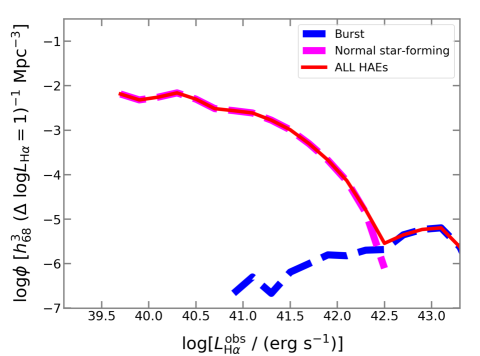
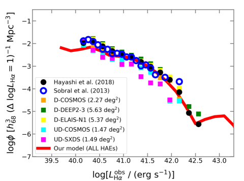
Figure 1: The H$\alpha$ LF (with the dust extinction) of the model HAEs (red solid line). Left: The H$\alpha$ LF of starburst HAEs (blue dashed line) and normal star-forming HAEs (magenta dashed line) are superimporsed. Right: Comparing the model H$\alpha$ LF with observed ones (non-dust corrected) at $z=0.4$ obtained by HiZELS (Sobral et al., 2013, blue open circles) and HSC-SSP (Hayashi et al., 2018, black filled circles: all the survey fields, colored squares: individual survey field). Note that Sobral et al. (2013) corrected dust attenuation by a simple way assuming 1 mag extinction for all HAEs. Thus we have plotted the observed LF by offsetting the corrected LF in Sobral et al. (2013); i.e., we have subtracted 0.4 dex from log$L_{\rm H\alpha}$ in their Table 4.

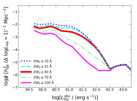
Figure 2: The H$\alpha$ LFs with various EW cuts. The red thick solid line show our standard model with $EW_{0}\geq 40$ Å. Thin lines indicate the LFs when we adopt other EW cut; specifically, blue dotted: $EW_{0}\geq 10$ Å (similar value to the observational study by Ly et al., 2007), cyan dashed: $EW_{0}\geq 25$ Å (the same as Sobral et al., 2013), green dashed-dotted: $EW_{0}\geq 70$ Å, and magenta solid: $EW_{0}\geq 100$ Å (the same as Drake et al., 2013). Other parameters are fixed; $f_{\rm neb}=0.5$ and $f_{\rm gas}\geq 0.10$.

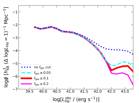
Figure 3: The H$\alpha$ LFs with various $f_{\rm gas}$ cuts. The thick solid red line show our standard model with $f_{\rm gas}\geq 0.10$. Thin lines indicate the LFs when we adopt other $f_{\rm gas}$ cut; specifically, blue dotted: without $f_{\rm gas}$ cut, cyan dashed: $f_{\rm gas}\geq 0.05$, and magenta solid: $f_{\rm gas}\geq 0.20$. Other parameters are fixed; $f_{\rm neb}=0.5$ and $EW_{0}\geq 40$ Å.

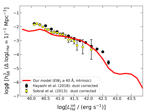
Figure 4: The intrinsic H$\alpha$ LF of the model HAEs (red solid line). Black and yellow filled circles show the observed LF corrected for the dust attenuation obtained by the HSC-SSP (Hayashi et al., 2018) and HiZELS (Sobral et al., 2013), respectively.

The left panel of Figure 1 shows the H$\alpha$ LF derived from our HAE model. The red solid line shows the H$\alpha$ LF derived by using all HAEs while magenta and blue dashed lines show H$\alpha$ LFs of normal star-forming HAEs and HAEs during starburst (hereafter starburst HAEs). As seen in the figure, normal star-forming HAEs dominate the fainter regime ($L_{\rm H\alpha}\lesssim 10^{42.5}$ erg s^-1) of the H$\alpha$ LF while starburst HAEs contribute the bright end of the LF.

In the right panel of Figure 1, we compare model H$\alpha$ LF (red solid line) with observed ones. Blue open circles show H$\alpha$ LF obtained by High-redshift(Z) Emission Line Survey (HiZELS; Sobral et al., 2013). The survey area of Sobral et al. (2013) is 2 deg². The filled circles and colored squares show H$\alpha$ LFs obtained by the HSC-SSP (Hayashi et al., 2018). The HSC-SSP HAE sample is obtained by utilizing NB921 images taken in two UltraDeep (UD) fields (UD-COSMOS and UD-SXDS fields) and three Deep (D) fields (D-COSMOS, D-DEEP2-3, and E-ELAIS-N1 fields). See Aihara et al. (2018b) and Hayashi et al. (2018) for further details of the survey. The H$\alpha$ LF shown by black filled circles is derived by using all HAEs in all of the survey fields (16.2 deg²) and those shown by colored squares are achieved in each individual field.

As seen in the figure, the observed H$\alpha$ LF in the individual HSC fields show a scatter up to $\sim$1 dex. The H$\alpha$ LFs from Sobral et al. (2013) and all of the survey fields of Hayashi et al. (2018) show no significant differences. Surprisingly, these two observational studies adopt different H$\alpha$ $EW_{0}$ thresholds to select HAEs, $EW_{0}\geq 40$ Å in Hayashi et al. (2018) and $EW_{0}\geq 25$ Å in Sobral et al. (2013). Figure 2 shows the model H$\alpha$ LFs with various EW cuts. When we adopt smaller EW cuts [10 Å and 25 Å; similar values to Ly et al. (2007) and Sobral et al. (2013), respectively], the H$\alpha$ LF does not show significant difference (up to $\sim$0.3 dex depending on the luminosity range; similar to the field variance as shown in Section 4), while the number density of HAEs is significantly lower than observed one in the case that we adopt $EW_{0}\geq$ 100 Å (the same as Drake et al., 2013). Presumably, the reason for these scatters and apparent agreement are given by the field variance. We discuss how the field variance affects the H$\alpha$ LF in Section 4.

In Figure 3, we show the dependence of the $f_{\rm gas}$ cut on the H$\alpha$ LF. Without the $f_{\rm gas}$ cut, the number density of model HAEs with $L_{\rm H\alpha}\gtrsim 10^{42}$ erg s^-1 is significantly higher than observed one. When we apply $f_{\rm gas}\geq$ 0.05 – 0.20, the H$\alpha$ LF shows no significant differences at $L_{\rm H\alpha}\lesssim 10^{42.3}$ erg s^-1. Based on the current observational dataset, we cannot restrict the bright end of the H$\alpha$ LF. When we discuss the field variance on the H$\alpha$ LF in Section 4, we focus on the number density of HAEs at $L_{\rm H\alpha}=10^{40.5}$ and $10^{41.5}$ erg s^-1 in which the LF is independent of the $f_{\rm gas}$ cut.

Figure 4 shows the intrinsic H$\alpha$ LF in the model compared with the dust corrected LF obtained by the HSC-SSP (Hayashi et al., 2018) and HiZELS (Sobral et al., 2013). Here model HAEs are selected by dust attenuated H$\alpha$ $EW_{0}$ and the intrinsic LF is derived by their intrinsic H$\alpha$ luminosities. Our model shows general agreement with the dust corrected LF of observed HAEs while the number density of model HAEs is slightly lower than those of observational results at the faint regime ($L_{\rm H\alpha}\lesssim 10^{41}$ erg s^-1). This difference may be due to difference in the extinction curves. As we described in subsection 2.1, the Calzetti law (Calzetti et al., 2000) is used in the $\nu^{2}$GC. On the other hand, Hayashi et al. (2018) estimate the amount of dust extinction based on the Balmer decrement by assuming the extinction curve by Cardelli et al. (1989). Moreover, Sobral et al. (2013) corrected dust attenuation by a simple way assuming 1 mag extinction for all HAEs. Since these differences have no significant impacts on the conclusion on the field variance, more detailed discussions will be a future work.

3.2 Model HAEs in the log($SFR$) – log($M_{\rm star}$) plane

We examine the relation between the SFR and stellar mass of model HAEs. Various previous observations have reported that star-forming galaxies show a tight correlation between their SFR and stellar mass, which is called the “main sequence (MS)” of star-forming galaxies (e.g., Elbaz et al., 2007; Noeske et al., 2007; Dunne et al., 2009; Santini et al., 2009; Kashino et al., 2013; Speagle et al., 2014; Boogaard et al., 2018). Therefore it is a good test to show the distribution of galaxies in the log(SFR) – log($M_{\rm star}$) plane for the reliability of our model.

The left panel of Figure 5 shows the log($SFR$) – log($M_{\rm star}$) plane of model HAEs. While normal star-forming HAEs are shown by magenta dots, starburst HAEs are denoted by blue circles. Model HAEs clearly show a tight correlation between SFR and stellar mass. The relation between the SFR and stellar mass can be fitted by an analytic function,

$${\rm log}[SFR/M_{\odot}{\rm yr}^{-1}]=\alpha_{\rm MS}{\rm log}[M_{\rm star}/M_{\odot}]+\beta_{\rm MS}.$$ (10)

The best-fit parameters are $\alpha_{\rm MS}=0.86\pm 0.02$ and $\beta_{\rm MS}=-8.26\pm 0.24$. The scatter in the log(SFR) direction is $\sigma_{\rm MS}=0.48\pm 0.18$. We compare our model HAE to observed MS of star-forming galaxies at similar redshift in the log($SFR$) – log($M_{\rm star}$) plane as shown in the right panel of Figure 5. The model well reproduces the MS of star-forming galaxies [Boogaard et al. (2018) at $z=0.4$: $\alpha_{\rm MS}=0.83$, $\beta_{\rm MS}=-7.96$ and $\sigma_{\rm MS}=0.44$; Sobral et al. (2014) at $0.39<z<0.41$: $\alpha_{\rm MS}=0.78$, $\beta_{\rm MS}=-7.78$ and $\sigma_{\rm MS}=0.49$]. Since model HAEs distribute along the observed main sequence, it is suggested that HAEs are typical MS galaxies.

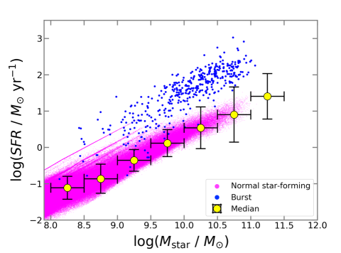
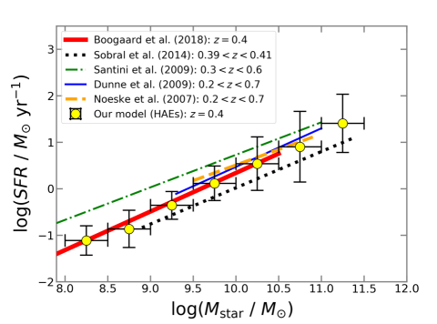
Figure 5: The log(SFR) – log($M_{\rm star}$) plane of HAEs($EW_{0}\geq 40$ Å). Left: Blue and magenta dots show starburst galaxies and normal star-forming galaxies, respectively. Yellow filled circles show median SFR in $M_{\rm star}$ bin ($\Delta$log$M_{\rm star}=0.5$). Error bars correspond to 1$\sigma$ standard deviation. Right: Comparison of SFR versus stellar mass relation of HAEs between our model and observational results. Observational results are shown by colored lines; red thick solid: Boogaard et al. (2018) ($z=0.4$), black dotted: Sobral et al. (2014) ($0.39<z<0.41$), green dashed-and-dotted: Santini et al. (2009) ($0.3<z<0.6$), blue thin solid: Dunne et al. (2009) ($0.2<z<0.7$), orange dashed: Noeske et al. (2007) ($0.2<z<0.7$).

3.3 The spatial distribution

We investigate how the HAE selection affects the spatial distribution of galaxies. Figure 6 shows the surface number density distribution of model galaxies with $r<-15$ mag (left) and HAEs with $L_{\rm H\alpha}\geq 10^{40}$ erg s^-1 (right) over $411.8\times 411.8$ Mpc² (corresponding to 14.8 $\times$ 14.8 deg²). We project a 411.8 Mpc $\times$ 411.8 Mpc region with a thickness of 70 Mpc (corresponding to the width of the HSC NB921 filter which is used to observe HAEs at $z=0.4$) to make a 2-dimensional image. Within a 411.8 Mpc $\times$ 411.8 Mpc $\times$ 70 Mpc region, there are 537,190 galaxies (SDSS $r<-15$ mag) and 67,808 HAEs ($L_{\rm H\alpha}\geq 10^{40}$ erg s^-1). The average surface number density of HAEs with $L_{\rm H\alpha}\geq 10^{40}$ erg s^-1 within a 411.8 Mpc $\times$ 411.8 Mpc $\times$ 70 Mpc box is 308.9 deg^-2. The local surface number density distribution is calculated by counting the number of galaxies within a fixed aperture with a radius of 1 Mpc. Both of all galaxies and HAEs show clear filamentary structure.

We then examine the overdensity $\delta$ distribution to investigate how HAEs trace the structure. The overdensity $\delta$ is defined as follows:

$$\delta\equiv\frac{n-\bar{n}}{\bar{n}},$$ (11)

where $n$ is the surface number density of galaxies within an aperture and $\bar{n}$ is the mean surface number density over the whole projected area. In Figure 7 we show the $\delta$ map of galaxies with $r<-15$ mag (left) and HAEs with $L_{\rm H\alpha}\geq 10^{40}$ erg s^-1 (right). The average and median of the surface number density of galaxies in an aperture are 3.04 Mpc^-2 and 1.59 Mpc^-2, while those of HAEs are 0.40 Mpc^-2 and 0.32 Mpc^-2. In each panel of Figure 7, regions in which the overdensity exceeds 5$\sigma$ are colored red. Clearly, the spatial distribution of HAEs shows higher overdensity in galaxy clusters and the filamentary structures compared to that of all galaxies, suggesting that HAEs are a good tracer to investigate structures such as cosmic filaments. We will examine the spatial distribution in more detail, including the clustering analysis, in a future paper.

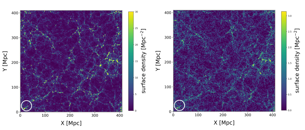
Figure 6: The surface number density distribution map of galaxies with $r<-15$ (left) and HAEs with $L_{\rm H\alpha}\geq 10^{40}$ erg s^-1 (right). White circles at left bottom in each map show the field-of-view of Subaru/HSC (1.5 degree diameter).

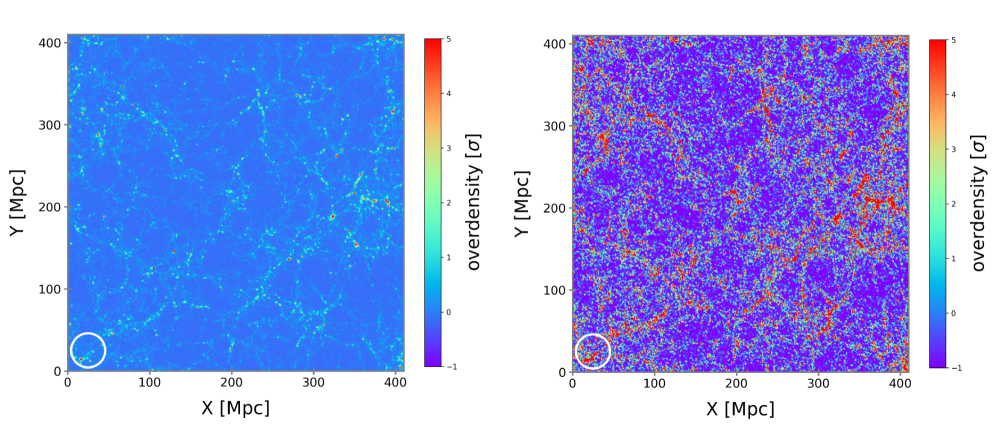
Figure 7: Overdensity ($\delta$) map of galaxies with $r<-15$ (left) and HAEs (right) with $L_{\rm H\alpha}\geq 10^{40}$ erg s^-1. Regions where the $\delta$ exceeds 5$\sigma$ are shown by red color in each map. White circles at left bottom in each map show the field-of-view of Subaru/HSC (1.5 degree diameter).

4 Field variance on the H$\alpha$ LF

In this section we discuss the field variance of the HAE distribution by focusing on the fluctuation of H$\alpha$ LFs in various environments. For this purpose, we divide the 411.8 Mpc $\times$ 411.8 Mpc field into square subregions and derive H$\alpha$ LFs in those regions. Figure 8 shows H$\alpha$ LFs derived by applying various areas of square region. In Figure 9, we show the frequency distribution of HAE number density, $\phi$, at $L_{\rm H\alpha}=10^{40.5}$ erg s^-1 (left) and at $10^{41.5}$ erg s^-1 (right). The spread of the LFs decreases with increasing survey the areas (see also Table 4). In the case of 2 deg² region (typical survey area of previous observations), the H$\alpha$ LF shows significantly large variance up to $\sim$1 dex. Therefore, any surveys narrower than 2 deg² could contain uncertainty of the number density at least $\sim$1 dex caused by the field variance. Furthermore, if a rare bright HAE is observed, the bright end of the LF could be overestimated by at least one order of magnitude, due to a small survey area.

In the left panel of Figure 10, we show the maximum ($\phi_{\rm max}$) and minimum ($\phi_{\rm min}$) number density of HAEs at a H$\alpha$ luminosity of $L_{\rm H\alpha}=10^{40.5}$ erg s^-1 (blue lines) and $10^{41.5}$ erg s^-1 (red lines) as a function of survey areas. These are also summarized in Table 4. In the right panel, differences between the logarithmic $\phi_{\rm max}$ and $\phi_{\rm min}$ at $L_{\rm H\alpha}=10^{40.5}$ erg s^-1 (blue line and filled squares) and at $10^{41.5}$ erg s^-1 (red line and filled circles) are shown. As seen in these figures, the differences monotonically decrease with increasing area size. The difference at $L_{\rm H\alpha}=10^{40.5}$ erg s^-1 (at $L_{\rm H\alpha}=10^{41.5}$ erg s^-1) is $\sim 0.7$ dex ($\sim 0.8$ dex) at the survey area of 2 deg² while it goes down to $\sim 0.25$ dex ($\sim 0.3$ dex) in the case of 15 deg² survey area, for instance. The number density differences as a function of the survey area, $A$ [Mpc²], are fitted by a power law function as follows:

$${\rm log}(\phi_{\rm max}/\phi_{\rm min})_{40.5}=(12.20\pm 1.40)\times A^{(-0.40\pm 0.02)}$$ (12)

at $L_{\rm H\alpha}=10^{40.5}$ erg s^-1 and

$${\rm log}(\phi_{\rm max}/\phi_{\rm min})_{41.5}=(63.80\pm 20.8)\times A^{(-0.58\pm 0.04)}$$ (13)

at $L_{\rm H\alpha}=10^{41.5}$ erg s^-1.

Finally, we focus on the standard deviation of the number density of HAEs in our model. Figure 11 shows the standard deviation ($\sigma_{\phi}$) at $L_{\rm H\alpha}=10^{40.5}$ erg s^-1 (blue) and $10^{41.5}$ erg s^-1 (red) as a function of $A$ [Mpc²]. We summarize $\sigma_{\phi}$ within some survey areas in Table 4 (the third column). $\sigma_{\phi}$ monotonically decreases with increasing area as well as the logarithmic $\phi$ difference. The relation between $\sigma_{\phi}$ and $A$ [Mpc²] can also be fitted by a power law:

$$\sigma_{\phi,40.5}=(1.20\pm 0.10)\times 10^{-2}\times A^{(-0.31\pm 0.01)}$$ (14)

at $L_{\rm H\alpha}=10^{40.5}$ erg s^-1 and

$$\sigma_{\phi,41.5}=(5.79\pm 0.21)\times 10^{-3}\times A^{(-0.38\pm 0.01)}$$ (15)

at $L_{\rm H\alpha}=10^{41.5}$ erg s^-1. In the case of 10 deg² survey, $\sigma_{\phi,40.5}\sim 8.0\times 10^{-4}$ and $\sigma_{\phi,41.5}\sim 1.8\times 10^{-4}$ while $\sigma_{\phi,40.0}\sim 1.3\times 10^{-3}$ and $\sigma_{\phi,41.5}\sim 3.6\times 10^{-4}$ in a 2 deg² survey.

Based on these examination, it is suggested that the dispersion of observed H$\alpha$ LFs and the apparent agreement in observational results with different HAE selection criteria could be explained by field variance. Equations (12) – (15) can be used for estimating how the field variance could affect observed LFs for a given survey area. Note that we have found that the H$\alpha$ LF shows a similar field variance even when we apply different set of parameters ($f_{\rm neb}$, $EW_{0}$, and $f_{\rm gas}$) and thus the parameter values do not affect our discussion.

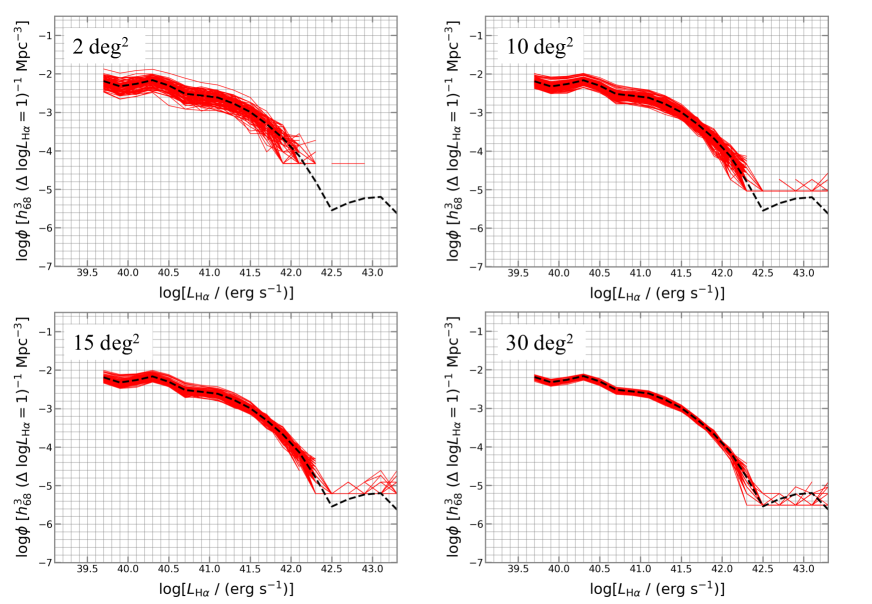
Figure 8: H$\alpha$ LFs within various survey area (red lines). Black dashed line in each panel shows the LF derived based on all HAEs in the (411.8 Mpc)³ box. 2, 10, 15, and 30 deg² correspond to $\sim$1,521, 3,844, 11,556, and 23,165 Mpc² in the comoving scale at $z=0.4$.

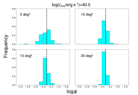
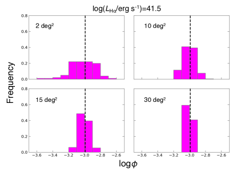
Figure 9: The frequency distribution of $\phi$ at $L_{\rm H\alpha}=10^{40.5}$ erg s^-1 (left panels) and $L_{\rm H\alpha}=10^{41.5}$ erg s^-1 (right panels). The survey areas shown here are the same as Figure 8. Vertical dashed line in each panel indicate the number density of HAEs in whole of (411.8 Mpc)³ box.

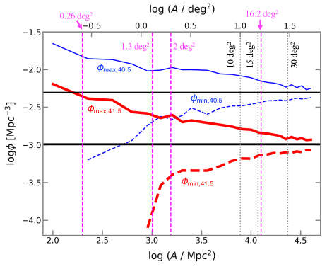
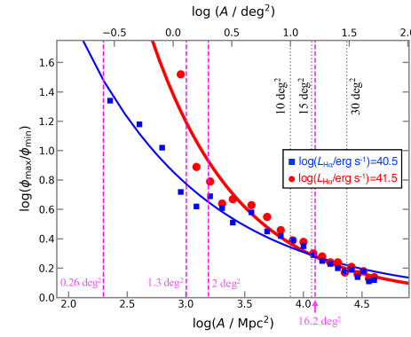
Figure 10: Left: The maximum (solid line) and minimum (dashed line) number density ($\phi$) of HAEs at H$\alpha$ luminosity of $L_{\rm H\alpha}=10^{40.5}$ erg s^-1 (blue) and at $L_{\rm H\alpha}=10^{41.5}$ erg s^-1 (red). The maximum ($\phi_{\rm max}$) and ($\phi_{\rm min}$) number density within some survey areas are summarized in Table 4. The black thin and thick horizontal lines indicate $\phi$ derived in whole of (411.8 Mpc)³ box at $L_{\rm H\alpha}=10^{40.5}$ erg s^-1 and $L_{\rm H\alpha}=10^{41.5}$ erg s^-1, respectively. Right: The difference between the maximum logarithmic number density ($\phi_{\rm max}$) and minimum one ($\phi_{\rm min}$) at $L_{\rm H\alpha}=10^{40.5}$ erg s^-1 (blue) and at $L_{\rm H\alpha}=10^{41.5}$ erg s^-1 (red). Filled blue squares and red circles show log($\phi_{\rm max}$/$\phi_{\rm min}$) calculated in square regions by changing the length of a side from 10 Mpc to 200 Mpc at intervals of 10 Mpc. The blue thin and red thick solid curves show a power law fits: ${\rm log}(\phi_{\rm max}/\phi_{\rm min})_{40.5}=(12.20\pm 1.40)\times A^{(-0.40\pm 0.02)}$ at $L_{\rm H\alpha}=10^{40.5}$ erg s^-1 and ${\rm log}(\phi_{\rm max}/\phi_{\rm min})_{41.5}=(63.80\pm 20.8)\times A^{(-0.58\pm 0.04)}$ at $L_{\rm H\alpha}=10^{41.5}$ erg s^-1. In each panel, vertical dotted lines show corresponding survey area in deg² while magenta ones denote survey areas of Ly et al. (2007) [0.26 deg²], Drake et al. (2013) [1.3 deg²], Sobral et al. (2011) [2 deg²], and Hayashi et al. (2018) [16.2 deg²].

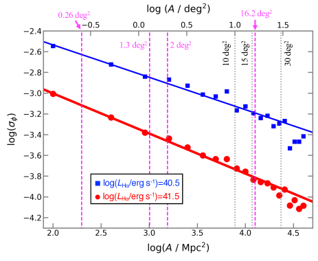
Figure 11: The standard deviation of the number density of HAEs at $L_{\rm H\alpha}=10^{40.5}$ erg s^-1 (filled blue squares) and 10^41.5 erg s^-1 (filled red circles) as a function of survey areas (the logarithm of the standard deviation of number density in the linear scale). $\sigma_{\phi}$ shown by filled blue squares and red circles are calculated in square regions by changing the length of a side from 10 Mpc to 200 Mpc at intervals of 10 Mpc. The blue and red solid lines show power law fits: $\sigma_{\phi,40.5}=(1.20\pm 0.10)\times 10^{-2}\times A^{(-0.31\pm 0.01)}$ at $L_{\rm H\alpha}=10^{40.5}$ erg s^-1 and $\sigma_{\phi,41.5}=(5.79\pm 0.21)\times 10^{-3}\times A^{(-0.38\pm 0.01)}$ at $L_{\rm H\alpha}=10^{41.5}$ erg s^-1, respectively. The vertical lines are the same as those in Figure 10.

Table 1: Summary of the field variance of the H$\alpha$ LFs within various survey areas.

at $L_{\rm H\alpha}=10^{40.5}$ erg s-1
Area [deg2]	$\phi_{\rm max}$ ($\times 10^{-3}$)	$\phi_{\rm min}$ ($\times 10^{-3}$)	$\sigma_{\phi}$ ($\times 10^{-3}$)
0.3	13.97	0.63	2.26
1.3	10.46	1.95	1.43
2.0	10.43	1.50	1.33
5.0	9.57	2.64	1.04
10.0	8.12	3.26	0.80
15.0	7.68	3.70	0.72
30.0	5.92	3.88	0.45
at $L_{\rm H\alpha}=10^{41.5}$ erg s-1
Area [deg2]	$\phi_{\rm max}$ ($\times 10^{-3}$)	$\phi_{\rm min}$ ($\times 10^{-3}$)	$\sigma_{\phi}$ ($\times 10^{-3}$)
0.3	4.13	0.00	0.71
1.3	2.44	0.21	0.40
2.0	2.44	0.28	0.36
5.0	1.95	0.46	0.25
10.0	1.66	0.64	0.18
15.0	1.53	0.71	0.16
30.0	1.22	0.81	0.10

5 Concluding Remarks

We have constructed a semi-analytic model of HAEs at $z=0.4$ based on the $\nu^{2}$GC to examine the field variance of the HAE distribution. We define the HAE in our model to be a galaxy with H$\alpha$ $EW_{0}\geq 40$ Å. To calculate the observed H$\alpha$ luminosity, we assume the dust attenuation level of the H$\alpha$ emission is higher than that of the continuum emission, $f_{\rm neb}=0.5$, as reported by observational studies at $z<1$. As for the starburst galaxies, we assume that only galaxies having significant gas fraction ($f_{\rm gas}\geq 0.1$) emit H$\alpha$ emission.

This model well reproduces the observed H$\alpha$ LFs at similar redshift ($z=0.4$). The relationship between the SFR and stellar mass of HAEs is also reproduced by the model. HAEs seem to be typical MS galaxies because they show a tight correlation between the SFR and stellar mass; ${\rm log}[SFR/M_{\odot}~{}{\rm yr}^{-1}]=(0.86\pm 0.02){\rm log}[M_{\rm star}/M_{\odot}]-(8.26\pm 0.24)$, with a scatter of $\sigma_{\rm MS}=0.48\pm 0.18$. In the model, the MS of HAEs is similar to that of galaxies with $sSFR\geq 10^{-10}$ yr^-1.

The (411.8 Mpc)³ comoving volume of $\nu^{2}$GC enables us to examine the spatial distribution of galaxies over a wide area. The surface number density of HAEs with $L_{\rm H\alpha}\geq 10^{40}$ erg s^-1 is 308.9 deg^-2. We have found that the HAE is a good tracer of the large-scale structure in the Universe because their spatial distribution shows significant overdensity ($>5\sigma$) in cluster environments and cosmic web filaments.

We have also examined the fluctuation of H$\alpha$ LFs derived in various survey areas. We have found that the H$\alpha$ LF derived by 2 deg² survey, typical area for previous observations, show significant field variance up to $\sim 1$ dex. In the case of wider surveys of $\gtrsim$15 deg², the field variance of LFs becomes smaller ($\lesssim$0.3 dex) and converge to the average LF derived in the whole (411.8 Mpc)³ box. The differences between maximum number density and minimum one can be fitted by a power law function, as well as the standard deviation of the LF given by Equations (12) – (15). Based on these, one can estimate the variance of the LF to examine whether or not the survey area is enough for their scientific goals.

This study shows that the $\nu^{2}$GC is so useful to examine various properties of galaxies over a wide area. We will construct HAE models at higher redshifts based on this study. Modeling other line emitters such as Ly$\alpha$ emitters, [O ii] emitters, and [O iii] emitters will be also done in future works. To examine the consistency between the model and observational outcomes, precious measurements of the line luminosity and EW are required. Further surveys with wide field spectroscopic instruments such as Prime Focus Spectrograph (Takada et al., 2014; Tamura et al., 2016, 2018) on the Subaru telescope are crucially important to progress our understandings on the nature of the galaxy evolution.

References

- Aihara et al. (2018a) Aihara, H., Arimoto, N., Armstrong, R., et al. 2018, PASJ, 70, S4
- Aihara et al. (2018b) Aihara, H., Armstrong, R., Bickerton, S., et al. 2018, PASJ, 70, S8
- Boogaard et al. (2018) Boogaard, L. A., Brinchmann, J., Bouché, N., et al. 2018, A&A, 619, A27
- Bruzual & Charlot (2003) Bruzual, G., & Charlot, S. 2003, MNRAS, 344, 1000
- Calzetti et al. (2000) Calzetti, D., Armus, L., Bohlin, R. C., et al. 2000, ApJ, 533, 682
- Cardelli et al. (1989) Cardelli, J. A., Clayton, G. C., & Mathis, J. S. 1989, ApJ, 345, 245
- Chabrier (2003) Chabrier, G. 2003, PASP, 115, 763
- Colbert et al. (2013) Colbert, J. W., Teplitz, H., Atek, H., et al. 2013, ApJ, 779, 34
- Darvish et al. (2014) Darvish, B., Sobral, D., Mobasher, B., et al. 2014, ApJ, 796, 51
- Durkalec et al. (2015) Durkalec, A., Le Fèvre, O., Pollo, A., et al. 2015, A&A, 583, A128
- de Lapparent et al. (1986) de Lapparent, V., Geller, M. J., & Huchra, J. P. 1986, ApJ, 302, L1
- Disney et al. (1989) Disney, M., Davies, J., & Phillipps, S. 1989, MNRAS, 239, 939
- Drake et al. (2013) Drake, A. B., Simpson, C., Collins, C. A., et al. 2013, MNRAS, 433, 796
- Dunne et al. (2009) Dunne, L., Ivison, R. J., Maddox, S., et al. 2009, MNRAS, 394, 3
- Elbaz et al. (2007) Elbaz, D., Daddi, E., Le Borgne, D., et al. 2007, A&A, 468, 33
- Enoki et al. (2014) Enoki, M., Ishiyama, T., Kobayashi, M. A. R., & Nagashima, M. 2014, ApJ, 794, 69
- Erb et al. (2006) Erb, D. K., Steidel, C. C., Shapley, A. E., et al. 2006, ApJ, 647, 128
- Garn et al. (2010) Garn, T., Sobral, D., Best, P. N., et al. 2010, MNRAS, 402, 2017
- Garn, & Best (2010) Garn, T., & Best, P. N. 2010, MNRAS, 409, 421
- Geach et al. (2008) Geach, J. E., Smail, I., Best, P. N., et al. 2008, MNRAS, 388, 1473
- Hayashi et al. (2010) Hayashi, M., Kodama, T., Koyama, Y., et al. 2010, MNRAS, 402, 1980
- Hayashi et al. (2013) Hayashi, M., Sobral, D., Best, P. N., et al. 2013, MNRAS, 430, 1042
- Hayashi et al. (2018) Hayashi, M., Tanaka, M., Shimakawa, R., et al. 2018, PASJ, 70, S17
- Hayashino et al. (2004) Hayashino, T., Matsuda, Y., Tamura, H., et al. 2004, AJ, 128, 2073
- Hatch et al. (2011) Hatch, N. A., Kurk, J. D., Pentericci, L., et al. 2011, MNRAS, 415, 2993
- Ho et al. (2012) Ho, S., Cuesta, A., Seo, H.-J., et al. 2012, ApJ, 761, 14
- Ishiyama et al. (2015) Ishiyama, T., Enoki, M., Kobayashi, M. A. R., et al. 2015, PASJ, 67, 61
- Kashino et al. (2013) Kashino, D., Silverman, J. D., Rodighiero, G., et al. 2013, ApJ, 777, L8
- Kennicutt (1998) Kennicutt, R. C., Jr. 1998, ARA&A, 36, 189
- Kewley et al. (2004) Kewley, L. J., Geller, M. J., & Jansen, R. A. 2004, AJ, 127, 2002
- Khostovan et al. (2015) Khostovan, A. A., Sobral, D., Mobasher, B., et al. 2015, MNRAS, 452, 3948
- Kodama et al. (2004) Kodama, T., Balogh, M. L., Smail, I., et al. 2004, MNRAS, 354, 1103
- Kodama et al. (2013) Kodama, T., Hayashi, M., Koyama, Y., et al. 2013, The Intriguing Life of Massive Galaxies, 74
- Koyama et al. (2011) Koyama, Y., Kodama, T., Nakata, F., et al. 2011, ApJ, 734, 66
- Koyama et al. (2013) Koyama, Y., Kodama, T., Tadaki, K.-. ichi ., et al. 2013, MNRAS, 428, 1551
- Koyama et al. (2019) Koyama, Y., Shimakawa, R., Yamamura, I., et al. 2019, PASJ, 71, 8
- Lee et al. (2012) Lee, J. C., Ly, C., Spitler, L., et al. 2012, PASP, 124, 782
- Ly et al. (2007) Ly, C., Malkan, M. A., Kashikawa, N., et al. 2007, ApJ, 657, 738
- Ly et al. (2011) Ly, C., Lee, J. C., Dale, D. A., et al. 2011, ApJ, 726, 109
- Makiya et al. (2016) Makiya, R., Enoki, M., Ishiyama, T., et al. 2016, PASJ, 68, 25
- Matsuda et al. (2004) Matsuda, Y., Yamada, T., Hayashino, T., et al. 2004, AJ, 128, 569
- Matsuda et al. (2011) Matsuda, Y., Smail, I., Geach, J. E., et al. 2011, MNRAS, 416, 2041
- Miyazaki et al. (2012) Miyazaki, S., Komiyama, Y., Nakaya, H., et al. 2012, Proc. SPIE, 84460Z
- Matthee et al. (2017) Matthee, J., Sobral, D., Best, P., et al. 2017, MNRAS, 471, 629
- Mawatari et al. (2012) Mawatari, K., Yamada, T., Nakamura, Y., et al. 2012, ApJ, 759, 133
- Moustakas et al. (2006) Moustakas, J., Kennicutt, R. C., & Tremonti, C. A. 2006, ApJ, 642, 775
- Nagashima et al. (2005) Nagashima, M., Yahagi, H., Enoki, M., Yoshii, Y., & Gouda, N. 2005, ApJ, 634, 26
- Noeske et al. (2007) Noeske, K. G., Weiner, B. J., Faber, S. M., et al. 2007, ApJ, 660, L43
- Oke & Gunn (1983) Oke, J. B., & Gunn, J. E. 1983, ApJ, 266, 713
- Ogura et al. (2017) Ogura, K., Nagao, T., Imanishi, M., et al. 2017, PASJ, 69, 51
- Ouchi et al. (2003) Ouchi, M., Shimasaku, K., Furusawa, H., et al. 2003, ApJ, 582, 60
- Ouchi et al. (2008) Ouchi, M., Shimasaku, K., Akiyama, M., et al. 2008, ApJS, 176, 301
- Ouchi et al. (2018) Ouchi, M., Harikane, Y., Shibuya, T., et al. 2018, PASJ, 70, S13
- Pannella et al. (2015) Pannella, M., Elbaz, D., Daddi, E., et al. 2015, ApJ, 807, 141
- Planck Collaboration et al. (2014) Planck Collaboration, Ade, P. A. R., Aghanim, N., et al. 2014, A&A, 571, A16
- Price et al. (2014) Price, S. H., Kriek, M., Brammer, G. B., et al. 2014, ApJ, 788, 86
- Puglisi et al. (2016) Puglisi, A., Rodighiero, G., Franceschini, A., et al. 2016, A&A, 586, A83
- Reddy et al. (2010) Reddy, N. A., Erb, D. K., Pettini, M., et al. 2010, ApJ, 712, 1070
- Ross et al. (2012) Ross, A. J., Percival, W. J., Sánchez, A. G., et al. 2012, MNRAS, 424, 564
- Santini et al. (2009) Santini, P., Fontana, A., Grazian, A., et al. 2009, A&A, 504, 751
- Schulze et al. (2009) Schulze, A., Wisotzki, L., & Husemann, B. 2009, A&A, 507, 781
- Shibuya et al. (2018) Shibuya, T., Ouchi, M., Konno, A., et al. 2018, PASJ, 70, S14
- Shimakawa et al. (2017) Shimakawa, R., Kodama, T., Hayashi, M., et al. 2017, MNRAS, 468, L21
- Shimasaku et al. (2003) Shimasaku, K., Ouchi, M., Okamura, S., et al. 2003, ApJ, 586, L111
- Shirakata et al. (2015) Shirakata, H., Okamoto, T., Enoki, M., et al. 2015, MNRAS, 450, L6
- Shirakata et al. (2019) Shirakata, H., Okamoto, T., Kawaguchi, T., et al. 2019, MNRAS, 482, 4846
- Sobral et al. (2011) Sobral, D., Best, P. N., Smail, I., et al. 2011, MNRAS, 411, 675
- Sobral et al. (2012) Sobral, D., Best, P. N., Matsuda, Y., et al. 2012, MNRAS, 420, 1926
- Sobral et al. (2013) Sobral, D., Smail, I., Best, P. N., et al. 2013, MNRAS, 428, 1128
- Sobral et al. (2014) Sobral, D., Best, P. N., Smail, I., et al. 2014, MNRAS, 437, 3516
- Sobral et al. (2015) Sobral, D., Matthee, J., Best, P. N., et al. 2015, MNRAS, 451, 2303
- Sobral et al. (2016) Sobral, D., Kohn, S. A., Best, P. N., et al. 2016, MNRAS, 457, 1739
- Somerville et al. (2004) Somerville, R. S., Lee, K., Ferguson, H. C., et al. 2004, ApJ, 600, L171
- Speagle et al. (2014) Speagle, J. S., Steinhardt, C. L., Capak, P. L., et al. 2014, ApJS, 214, 15
- Springel et al. (2005) Springel, V., White, S. D. M., Jenkins, A., et al. 2005, Nature, 435, 629
- Stott et al. (2013) Stott, J. P., Sobral, D., Bower, R., et al. 2013, MNRAS, 436, 1130
- Stroe et al. (2014) Stroe, A., Sobral, D., Röttgering, H. J. A., et al. 2014, MNRAS, 438, 1377
- Stroe et al. (2017) Stroe, A., Sobral, D., Paulino-Afonso, A., et al. 2017, MNRAS, 465, 2916
- Sutherland & Dopita (1993) Sutherland, R. S., & Dopita, M. A. 1993, ApJS, 88, 253
- Suzuki et al. (2016) Suzuki, T. L., Kodama, T., Sobral, D., et al. 2016, MNRAS, 462, 181
- Takada et al. (2014) Takada, M., Ellis, R. S., Chiba, M., et al. 2014, PASJ, 66, R1
- Tamura et al. (2016) Tamura, N., Takato, N., Shimono, A., et al. 2016, Proc. SPIE, 99081M
- Tamura et al. (2018) Tamura, N., Takato, N., Shimono, A., et al. 2018, Proc. SPIE, 107021C
- Tanaka et al. (2011) Tanaka, I., De Breuck, C., Kurk, J. D., et al. 2011, PASJ, 63, 415
- Trenti & Stiavelli (2008) Trenti, M., & Stiavelli, M. 2008, ApJ, 676, 767
- Valentino et al. (2015) Valentino, F., Daddi, E., Strazzullo, V., et al. 2015, ApJ, 801, 132
- White & Frenk (1991) White, S. D. M., & Frenk, C. S. 1991, ApJ, 379, 52
- Wuyts et al. (2011) Wuyts, S., Förster Schreiber, N. M., Lutz, D., et al. 2011, ApJ, 738, 106