Repetition-based NOMA Transmission and Its Outage Probability Analysis

Abstract

In this paper, we discuss a non-orthogonal multiple access (NOMA) scheme to exploit a high diversity gain using repetition, namely repetition-based NOMA. Unlike conventional power-domain NOMA, all the users can have the same transmit power, but different number of repetitions. Thanks to a high diversity gain, a low outage probability can be achieved without instantaneous channel state information (CSI) feedback for power allocation. A closed-form expression for an upper-bound on the outage probability is derived so that the values of key parameters can be decided to maintain the outage probability below a target value. We also consider the average error probability for finite-length codes. Simulation results are compared with the derived bounds and it is shown that the bounds are reasonably tight and can be used to decide key parameters (e.g., code rates) to guarantee target error probabilities.

I Introduction

Since non-orthogonal multiple access (NOMA) has a higher spectral efficiency than orthogonal multiple access (OMA), it has been extensively studied [1] [2], although there are a number of challenges (e.g., optimal user clustering [3] and beamforming [4] [5]). In [6] [7], the notion of NOMA can be employed in uncoordinated transmissions such as random access for uplink transmissions in order to improve the throughput, which is important for massive machine-type communication (MTC) that provides the connectivity for various Internet-of-Things (IoT) applications [8].

In this paper, we consider a NOMA scheme that can have a low outage probability without channel state information (CSI) feedback so that it can be used for low-latency communication in MTC (thanks to no CSI feedback as well as a low outage probability). In conventional power-domain NOMA, the power allocation based on instantaneous CSI is essential for successful successive interference cancellation (SIC). If instantaneous CSI is not available, the power allocation can be carried out with statistical CSI to maximize the throughput as in [9] (in [10] for downlink). In this case, there might be a delay due CSI feedback, and outage events (due to fading) and error propagation in SIC are inevitable. As a result, for reliable transmissions, re-transmissions are required and the resulting access delay becomes random and can be long. Furthermore, as in [11], when instantaneous CSI can be available using limited CSI feedback, due to quantization error and delay [12], CSI becomes imperfect, which leads to outage events and error propagation in SIC. Thus, if power-domain NOMA is applied to low-latency communication under time-varying fading (with statistical CSI or limited CSI feedback), there might be outage events. To keep the outage probability low without instantaneous CSI-based power allocation, we consider repetition-based NOMA that exploits a high diversity gain. The main difference from other power-domain NOMA with statistical CSI (e.g., [9] [10]) is that the gain from NOMA is used to lower the outage probability rather than to increase the spectral efficiency.

In order to guarantee a certain low error probability, good performance prediction techniques are required so that the key parameters of repetition-based NOMA can be decided in advance. To this end, we focus on deriving a tight bound on the outage probability as a closed-form expression in this paper. In uplink NOMA, other users’ signals become interfering signals and their strength depends on fading, which makes the interference power a random variable. Since its probability density function (pdf) is unknown, we consider an approximation with the chi-squared distribution under Rayleigh fading by using a moment matching approach. Based on this approximation, we obtain an upper-bound on the outage probability with finite-length codes [13]. We also study decoding error probability for finite-length codes using the derived outage probability. Simulation results show that this bound is tight at a low outage probability. Thus, key parameters (e.g., the code rates) can be determined to keep a low outage probability or a high probability of successful SIC.

In summary, the main contributions are two-fold: i) repetition-based NOMA is proposed to exploit a high diversity gain for a low error probability without instantaneous CSI-based power allocation for low-latency communication; ii) a closed-form expression for the outage probability is derived, which allows to decide key parameters of repetition-based NOMA for a desirable performance (i.e., a certain low error rate).

The rest of the paper is organized as follows. In Section II, we present the system model for repetition-based NOMA to be used for uplink transmissions. To see the performance of repetition-based NOMA in terms of key parameters, we analyze the performance and find a tight upper-bound on the outage probability in Section III. The error probability with finite-length codes is studied in Section IV. Simulation results are presented in Section V together with the bounds, which can help determine design criteria for repetition-based NOMA. The paper is concluded with some remarks in Section VI.

Notation

Matrices and vectors are denoted by upper- and lower-case boldface letters, respectively. The superscripts ${\rm T}$ and ${\rm H}$ denote the transpose and complex conjugate, respectively. The Kronecker delta is denoted by $\delta_{l,l^{\prime}}$, which is 1 if $l=l^{\prime}$ and 0 otherwise. ${\mathbb{E}}[\cdot]$ and ${\rm Var}(\cdot)$ denote the statistical expectation and variance, respectively. ${\cal C}{\cal N}({\bf a},{\bf R})$ represents the distribution of circularly symmetric complex Gaussian (CSCG) random vectors with mean vector ${\bf a}$ and covariance matrix ${\bf R}$. The Q-function is given by ${\cal Q}(x)=\int_{x}^{\infty}\frac{1}{\sqrt{2\pi}}e^{-\frac{t^{2}}{2}}dt$.

II System Model

In this section, we consider a NOMA scheme for uplink based on repetition with multiple radio resource blocks. As in [14], each block can be seen as a time-frequency resource block and it is assumed that a signal transmitted through a block experiences an independent block fading [15]. Unlike conventional power-domain NOMA schemes, it is assumed that the average receive powers of users’ signals in the proposed scheme are the same (to this end, open-loop power control can be used, where each user can set its transmit power based on the average power of the received signal from a base station (BS) based on statistical channel reciprocity [16]). Thus, the proposed scheme may be suitable for uplink with users who cannot arbitrarily increase the transmit power for power-domain NOMA and a BS that does not perform instantaneous CSI-based power allocation.

Suppose that we have a set of $L$ parallel radio resource blocks (in the frequency domain), which is called a frame, for uplink transmissions. A frame is to be shared by multiple users in uplink transmissions for a high spectral efficiency based on NOMA. For NOMA, there are multiple layers and a user can transmit a different number of copies of a packet depending on his/her layer, where each layer is characterized by the number of copies per user and users in the same layer need to transmit their copies through different (orthogonal) blocks. In each block, there are $B$ signals transmitted (one signal from each layer), where $B$ represents the number of layers that are generated by power-domain NOMA. For example, as shown in Fig. 1, with a frame consisting of 4 blocks, we can have 3 layers. A user in layer 1 is to transmit 4 copies of a packet through all 4 blocks. There are two users in layer 2 and each user is to transmit two copies of a packet through two blocks. In layer 3, there are 4 users and each user is to transmit a packet through a block. In this example, in each frame consisting of 4 block, there are 7 users in a frame and 3 co-existing signals per block, which clearly shows that the resulting scheme is a NOMA scheme. For convenience, the resulting scheme is referred to as repetition-based NOMA.

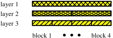
Figure 1: A layered structure of frame with 3 layers and 4 blocks.

At the BS, the signals can be decoded with SIC as other NOMA schemes. In this paper, it is assumed that a signal in a lower layer transmits more copies (repetitions) than that in a higher layer. Thus, the BS is to decode the signals from layer 1 to layer $B$ with SIC, where $B$ represents the number of layers. From this, for successful SIC with a high probability, it is expected that the probability of decoding error is the lowest in layer 1 and might increase with $b\in\{1,\ldots,B\}$, where $b$ represents the layer index, thanks to the diversity gain. Although there can be as many as layers, the number of layers, $B$, has to be limited, while $B$ needs to be proportional to $L$ for a high spectral efficiency.

Suppose that user $k$ is in layer $1$. Let ${\cal U}_{l}$ be the index set of the users transmitting signals through the $l$th block. In addition, denote by ${\cal L}_{k}$ the index set of the blocks that are used for multiple transmissions by user $k$. Then, the received signal at the BS through the $l$th block is given by

$${\bf r}_{l}=h_{l,k}{\bf s}_{l,k}+\sum_{q\in{\cal U}_{l}\setminus k}h_{l,q}{\bf s}_{l,q}+{\bf n}_{l},\ l\in{\cal L}_{k},$$ (1)

where $h_{l,k}$ represents the channel coefficient from user $k$ to the BS through the $l$th block, ${\bf s}_{l,k}$ is the $l$th copy of the signal packet transmitted (through the $l$th block) by the $k$th user, and ${\bf n}_{l}\sim{\cal C}{\cal N}({\bf 0},N_{0}{\bf I})$ represents the background noise vector. For example, in Fig. 1, with $L=4$ and $B=3$, suppose that user 1 lies in layer 1 and transmits signals through blocks ${\cal L}_{1}=\{1,2,3,4\}$. In addition, let users 2 and 3 be in layer 2 with ${\cal L}_{2}=\{1,2\}$ and ${\cal L}_{3}=\{3,4\}$, respectively, and let users 4, 5, 6, and 7 be in layer 3 with ${\cal L}_{4}=\{1\}$, ${\cal L}_{5}=\{2\}$, ${\cal L}_{6}=\{3\}$, and ${\cal L}_{7}=\{4\}$, respectively. In this case, with $k=1$, we have ${\cal U}_{1}\setminus k=\{2,4\}$, ${\cal U}_{2}\setminus k=\{2,5\}$, ${\cal U}_{3}\setminus k=\{3,6\}$, and ${\cal U}_{4}\setminus k=\{3,7\}$.

It is assumed that the $l$th copy of user $k$’s signal is an interleaved block of the original signal block, denoted by ${\bf s}_{k}$, i.e.,

$${\bf s}_{l,k}=\Pi_{l,k}({\bf s}_{k}),$$ (2)

where $\Pi_{l,k}(\cdot)$ denotes the interleaving operation for the $l$th copy at user $k$. In particular, a random permutation can be considered for the interleaving operation. In this case, $\Pi_{l,k}$ is seen as a random permutation matrix. For convenience, let $\Pi^{-1}_{l,k}$ be the deinterleaving operation. Throughout the paper, we also assume that ${\mathbb{E}}[{\bf s}_{k}]={\bf 0}$ and ${\mathbb{E}}[{\bf s}_{k}{\bf s}_{q}^{\rm H}]=P{\bf I}\delta_{k,q}$, where $P$ represents the signal power of all users.

At the BS, the decoding order with SIC corresponds to the number of layer, $b$, as mentioned earlier. That is, the signals in layer 1 are to be decoded first. To decode the signal from user $k$, the maximal ratio combining (MRC) [17] [18] is used with deinterleaved signals as follows:

$${\bf y}_{k} =\sum_{l\in{\cal L}_{k}}h_{l,k}^{*}\Pi^{-1}_{l,k}({\bf r}_{l})$$ (3)

$$=\sum_{l\in{\cal L}_{k}}|h_{l,k}|^{2}{\bf s}_{k}+\sum_{l\in{\cal L}_{k}}h_{l,k}^{*}{\bf w}_{l,k},$$ (4)

where

$${\bf w}_{l,k}=\sum_{q\in{\cal U}_{l}\setminus k}h_{l,q}\Pi_{l,k}^{-1}({\bf s}_{l,q})+\Pi_{l,k}^{-1}({\bf n}_{l}).$$ (5)

Once all the signals in layer 1 are decoded, they can be removed from ${\bf r}_{l}$ using SIC. Then, the BS is to decode the signals in layer 2, and so on. In this case, ${\cal U}_{l}$ is to be updated by removing the indices of the users in layer 1 because their signals in layer 1 are removed.

Decoding can be unsuccessful, which incurs error propagation and outage events due to incorrect SIC operation [9] (which is also true for downlink NOMA as in [10]). Thus, it might be important to guarantee successful decoding with a high probability. To this end, it is necessary to have a sufficient number of repetitions or copies for a high diversity gain.

In repetition-based NOMA, since the powers are fixed and no power allocation is carried out, we consider rate allocation for successful decoding with a sufficiently high probability. To this end, it is necessary to know the error probability in terms of the code rate and other parameters. In the next sections, we will focus on the derivation of the error rate.

III Performance Analysis

To guarantee a specific target error probability and decide key parameters (e.g., the code rate) accordingly at each layer, we need to predict the performance under given conditions. To this end, in this section, we focus on the performance analysis with the outage probability to allow such a prediction.

III-A Outage Probability

In this subsection, we assume that the number of copies for user $k$ is $D=|{\cal L}_{k}|$. In addition, it is assumed that all the interfering signals in the lower layers are removed by successful SIC. To find a closed-form expression for the outage probability, the following assumptions are mainly considered:

• The interleaving operation makes the copies of the signal ${\bf s}_{k}$ uncorrelated, i.e.,

  $${\mathbb{E}}[\Pi_{l,k}({\bf s}_{k})(\Pi_{l^{\prime},q}({\bf s}_{q}))^{\rm H}] =P{\bf I}\delta_{l,l^{\prime}}\delta_{k,q}$$ (6)

  $${\mathbb{E}}[\Pi_{l,k}^{-1}({\bf s}_{k})(\Pi_{l^{\prime},q}^{-1}({\bf s}_{q}))^{\rm H}] =P{\bf I}\delta_{l,l^{\prime}}\delta_{k,q}.$$ (7)

• The channels are independent Rayleigh fading channels with

  $${\mathbb{E}}[h_{l,k}h_{l^{\prime},q}^{*}]=\sigma_{h}^{2}\delta_{l,l^{\prime}}\delta_{k,q}.$$ (8)

  Thus, $X_{l,k}=|h_{l,k}|^{2}$ has the following exponential distribution:

  $$X_{l,k}\sim{\rm Exp}(\sigma_{h}^{2})=\frac{1}{\sigma_{h}^{2}}\exp\left(-\frac{X_{l,k}}{\sigma_{h}^{2}}\right),\ X_{l,k}\geq 0.$$ (9)

Under the assumption of A1, we have

$${\mathbb{E}}[\Pi_{l,k}^{-1}({\bf s}_{l,q})(\Pi_{l,k}^{-1}({\bf s}_{l,q^{\prime}}))^{\rm H}]=P{\bf I}\delta_{q,q^{\prime}}.$$ (10)

From this, it can be shown that

$${\mathbb{E}}[{\bf w}_{l,k}{\bf w}_{l^{\prime},k}^{\rm H}]=\left(\sum_{q\in{\cal U}_{l}\setminus k}X_{l,q}P{\bf I}+N_{0}\right)\delta_{l,l^{\prime}}.$$ (11)

The instantaneous signal-to-interference-plus-noise ratio (SINR) for user $k$ in (4) becomes

$$\gamma_{k} =\frac{(\sum_{l=1}^{D}X_{l,k})^{2}P}{\sum_{l=1}^{D}X_{l,k}(N_{0}+P\sum_{q\in{\cal U}_{l}\setminus k}X_{l,q})}$$ (12)

$$=\frac{\sum_{l=1}^{D}X_{l,k}P}{\frac{\sum_{l=1}^{D}(\sum_{q\in{\cal U}_{l}\setminus k}X_{l,q})X_{l,k}}{\sum_{l=1}^{D}X_{l,k}}P+N_{0}}.$$ (13)

Let $T_{k}$ denote the SINR threshold for successful decoding. Then, the outage probability becomes

$${\mathbb{P}}_{k}=\Pr(\gamma_{k}<T_{k}).$$ (14)

Thus, we need to find the distribution of the instantaneous SINR, $\gamma_{k}$.

III-B SINR Analysis

For convenience, let $M=|{\cal U}_{l}\setminus k|$, i.e., the number of the interfering signals is denoted by $M$. If $M=0$, under the assumption of A2 or from (9), we can show that

$$\sum_{l=1}^{D}X_{l,k}=\frac{\sigma_{h}^{2}\chi_{2D}^{2}}{2},$$ (15)

where $\chi_{n}^{2}$ represents a chi-squared random variable with $n$ degrees of freedom. For convenience, let $Z_{n}=\frac{\chi_{2n}^{2}}{2n}$. Then, it follows

$$\Pr(\gamma_{k}<T_{k})=\Pr\left(Z_{D}<\frac{T_{k}}{D{\sf SNR}}\right),$$ (16)

where ${\sf SNR}=\frac{P\sigma_{h}^{2}}{N_{0}}$ is the signal-to-noise ratio (SNR). Thus, using the cumulative distribution function (cdf) of the chi-squared random variable, the outage probability can be found. Furthermore, as shown in Appendix B, the following tight upper-bound on the outage probability can be obtained:

$$\Pr(\gamma_{k}<T_{k})\leq\frac{1}{D!}\left(\frac{T_{k}}{{\sf SNR}}\right)^{D}e^{-\frac{c_{D}T_{k}}{{\sf SNR}}}\leq\frac{1}{D!}\left(\frac{T_{k}}{{\sf SNR}}\right)^{D},$$ (17)

where

$$c_{D}=De^{-1}\left(D!\right)^{-\frac{1}{D}}\leq 1.$$ (18)

Unfortunately, if $M>0$, it is difficult to obtain a bound on the outage probability. Thus, we have to resort to an approximation. For convenience, let the interference term in (13) be

$$P\frac{\sum_{l=1}^{D}(\sum_{q\in{\cal U}_{l}\setminus k}X_{l,q})X_{l,k}}{\sum_{l=1}^{D}X_{l,k}}=\frac{P\sigma_{h}^{2}}{2}\sum_{l=1}^{D}Y_{l}\alpha_{l},$$ (19)

where $\alpha_{l}=\frac{X_{l,k}}{\sum_{l=1}^{D}X_{l,k}}\geq 0$ with $\sum_{l=1}^{D}\alpha_{l}=1$, and $Y_{l}=\frac{2}{\sigma_{h}^{2}}\sum_{q\in{\cal U}_{l}\setminus k}X_{l,q}$. Clearly, $Y_{l}$ is a chi-squared random variables with $2M$ degrees of freedom. Let $W=\sum_{l=1}^{D}\alpha_{l}Y_{l}$. If $\alpha_{l}=\frac{1}{D}$ for all $l$, we can see that $W$ becomes a scaled chi-squared random variable with $2DM$ degrees of freedom. However, since $\alpha_{l}$ is a random variable, the resulting approximation may have a lower variance than the actual one. Since $W$ can be seen as a weighted sum of chi-squared random variables, we may consider another chi-squared random variable to approximate $W$. To this end, let

$$\Omega=\frac{\chi_{2NM}^{2}}{N},$$ (20)

where $N$ is a parameter to be decided using a moment matching approach. It can be shown that ${\mathbb{E}}[W]={\mathbb{E}}\left[\sum_{l=1}^{D}\alpha_{l}Y_{l}\right]=2M$, because ${\mathbb{E}}[\chi_{2n}^{2}]=2n$. In addition, ${\mathbb{E}}[\Omega]=2M$. Thus, regardless of the value of $N$, we can see that $W$ and $\Omega$ have the same mean. We can consider the 2nd moment and find $N$ such that

$${\mathbb{E}}[W^{2}]={\mathbb{E}}[\Omega^{2}].$$ (21)

Lemma 1

The value of $N$ satisfying (21) is given by

$$N=\frac{D+1}{2}.$$ (22)

Proof:

See Appendix A. ∎

In Fig. 2, the empirical cdf of $W$ is shown with the cdf of $\Omega$ for two different pairs of $M$ and $D$. Clearly, thanks to the moment matching (up to the 2nd moment), the two cdfs become quite similar to each other.

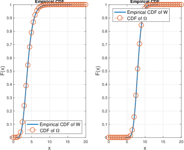
Figure 2: Empirical cdf of $W$ and an approximate cdf with $\Omega$: (a) $(D,M)=(8,2)$; (b) $(D,M)=(32,4)$.

By replacing $W$ with $\Omega$, the instantaneous SINR in (13) can be approximated as

$$\gamma_{k}\approx\frac{\sum_{l=1}^{D}X_{l,k}P}{\frac{P\sigma_{h}^{2}}{2}\Omega+N_{0}}.$$ (23)

For a tractable analysis, the instantaneous SINR in (23) can be used.

III-C A Closed-form Expression for Outage Probability

In this subsection, we find a closed-form expression for the outage probability with the SINR in (23). Since $\Omega$ is a (scaled) chi-squared random variable with $2NM$ degrees of freedom, the outage probability in (14) can have the following approximation:

$${\mathbb{P}}_{k} =\Pr(\gamma_{k}<T_{k})$$ (24)

$$\approx\tilde{\mathbb{P}}_{k}=\Pr\left(Z_{D}<\frac{T_{k}}{D}\left(\frac{\chi_{2NM}^{2}}{2N}+\frac{1}{{\sf SNR}}\right)\right).$$ (25)

We can have a closed-form expression for $\tilde{\mathbb{P}}_{k}$ as follows.

Lemma 2

For $M\geq 1$, suppose that

$$d=\frac{D}{c_{D}T}-\frac{1}{{\sf SNR}}>0,$$ (26)

where $T=T_{k}$ (for convenience, we omit the index $k$). Then, we have

$$\tilde{\mathbb{P}}_{k}\leq\psi(D,M,{\sf SNR},T)+\left(\frac{de}{M}\right)^{MN}e^{-Nd},$$ (27)

where

$$\psi(D,M,{\sf SNR},T)=\frac{1}{D!}\left(\frac{T}{{\sf SNR}}\right)^{D}\frac{e^{-\frac{c_{D}T}{{\sf SNR}}}}{(1+\frac{c_{D}T}{N})^{MN}}$$ (28)

$$\quad\times\sum_{n=0}^{D}\binom{D}{n}\left(\frac{{\sf SNR}}{N+c_{D}T}\right)^{n}\prod_{t=0}^{n-1}(MN+t).$$ (29)

Since the 2nd term on the right-hand side (RHS) in (27) is negligible if $d$ is sufficiently large, the first term becomes a good approximation of $\tilde{\mathbb{P}}_{k}$.

Proof:

See Appendix B. ∎

For the outage probability, we will usually consider the first term on the RHS in (27) (for a large $d$). Note that in (17), we can see that the diversity gain is $D$ as the outage probability is proportional to ${\sf SNR}^{-D}$ when $M=0$. For the case of $M\geq 1$, in order to see the diversity gain, we have the following result.

Lemma 3

Suppose that (26) holds. Then, it can be shown that

$$\psi\leq\frac{C}{D!}\nu^{D},$$ (30)

where $C$ is a constant that is independent of $D$ and $\nu$ becomes smaller than 1 if

$$\frac{{\sf SNR}}{T}\left(\frac{D+1}{D+1+2c_{D}T}\right)^{\frac{M}{2}}\geq 1+{\sf SNR}\frac{D(M+1)+M-1}{D+1+2c_{D}T}.$$ (31)

Proof:

See Appendix C. ∎

In (30), taking $\frac{1}{\nu}$ as a scaled SINR, we can see that the diversity gain becomes $D$. In general, we can derive design criteria for repetition-based NOMA to keep the outage probability low from (29) (or to hold (31)). However, since the expression in (29) is a bit complicated, it is not easy to obtain design criteria. Thus, for a more tractable analysis, we can consider the asymptotic $\psi$ when ${\sf SNR}\to\infty$ as follows.

Lemma 4

If $M\geq 1$, we have

$$\bar{\psi} =\lim_{{\sf SNR}\to\infty}\psi(D,M,{\sf SNR},T)$$ (32)

$$=\binom{MN+D-1}{MN-1}\left(\frac{N}{N+c_{D}T}\right)^{MN}\left(\frac{T}{N+c_{D}T}\right)^{D}.$$ (33)

Proof:

See Appendix D. ∎

From (33), when $D$ increases with a fixed $\rho=\frac{T}{N}$, since $\binom{n}{m}\leq 2^{n{\sf H}(m/n)}$, where ${\sf H}(p)=-p\log_{2}p-(1-p)\log_{2}(1-p)$, we can further show that

$$\bar{\psi} \leq 2^{(MN+D-1){\sf H}\left(\frac{MN-1}{MN+D-1}\right)}\left(\frac{\rho}{1+c_{D}\rho}\right)^{D}\left(\frac{1}{1+c_{D}\rho}\right)^{MN}$$ (34)

$$\approx 2^{D\left(1+\frac{M}{2}\right){\sf H}\left(\frac{M}{M+2}\right)}\left(\frac{\rho}{\left(1+\rho\right)^{1+\frac{M}{2}}}\right)^{D},$$ (35)

where the approximation is tight if $D$ is sufficiently large with $N=\frac{D+1}{2}$ and $c_{D}\to 1$. From this, it can be further shown that

$$\frac{\log_{2}\bar{\psi}}{D} =\left(1+\frac{M}{2}\right)\left({\sf H}\left(\frac{M}{M+2}\right)-\log_{2}(1+\rho)\right)$$ (36)

$$\quad+\log_{2}\rho.$$ (37)

This implies that if

$${\sf H}\left(\frac{M}{M+2}\right)<\log_{2}(1+\rho)-\frac{\log_{2}\rho}{1+\frac{M}{2}}$$ (38)

holds, $\bar{\psi}$ decreases exponentially with $D$ (i.e., the diversity order is $D$). Since ${\sf H}(p)\leq 1$, a sufficient condition for (38) can be found as follows:

$$2^{1+\frac{M}{2}}<\frac{1}{\rho}=\frac{N}{T}=\frac{D+1}{2T}.$$ (39)

For convenience, let $D_{(b)}$ and $M_{(b)}$ denote the number of copies and the number of interfering signals for a user in layer $b$, respectively, and assume that all the users in a layer have the same number of copies and the same number of interfering signals. Then, according to (39), with a sufficiently high SNR, at layer $b$, a low outage probability is expected in repetition-based NOMA if

$$M_{(b)}\leq 2\log_{2}\frac{D_{(b)}}{4T_{(b)}},$$ (40)

where $T_{(b)}$ is the threshold for the users in layer $b$. In addition, since $M_{(b)}$ decreases with $b$, the number of copies in layer $b$, $L_{(b)}$, needs to be larger than that in layer $b^{\prime}$ if $b<b^{\prime}$, as illustrated in Fig. 1.

In order to determine key parameters, from (40), with a fixed $T_{(b)}=T$ for all layers, we can show that

$$D_{(b)}=4T2^{\frac{M_{(b)}}{2}}\propto 2^{\frac{B-b}{2}},$$ (41)

since $M_{(b)}=B-b$. From (41), we can see that the number of copies can decrease exponentially with $b$. In addition, the number of blocks, $L$, has to be proportional to $2^{B}$, which means that the number of layers, $B$, cannot be arbitrarily large with respect to a finite $L$. A small $B$ (e.g., $B\leq 3$) is also important to keep SIC error propagation limited. Since $L=D_{(b)}K_{(b)}$, where $K_{(b)}$ represents the number of users in layer $b$, we also have $K_{(b)}\propto 2^{\frac{b}{2}}$.

III-D Other Issues

If $B=1$ (i.e., orthogonal multiple access (OMA) is used), each user has the outage probability as in (17). However, if we consider $B>1$ (i.e., NOMA) for a higher spectral efficiency, the performance of layer $b$ is affected by the performance of layers $1,\ldots,b-1$ through error propagation. To see the impact of imperfect SIC through error propagation on performance, consider the error probability with SIC propagation. Let $\epsilon_{b}$ denote the outage probability of the signal in layer $b$. Then, the error probability with SIC propagation at each layer, denoted by $\rho_{b}$, becomes

$$\rho_{1} =\epsilon_{1}$$

$$\rho_{2} =(1-\epsilon_{1})\epsilon_{2}+\epsilon_{1}\leq\epsilon_{1}+\epsilon_{2}$$

$$\rho_{3} =\epsilon_{1}+(1-\epsilon_{1})\epsilon_{2}+(1-\epsilon_{1})(1-\epsilon_{2})\epsilon_{3}\leq\epsilon_{1}+\epsilon_{2}+\epsilon_{3}$$

$$\vdots$$

Thus, the error probability with SIC propagation is bounded by $\sum_{b=1}^{B}\epsilon_{b}$ or $O(\max_{b}\epsilon_{b})$ if $B$ is sufficiently small (e.g., 3 or 4), which implies that the impact of error propagation on the performance may not be significant. To see further, suppose that $T_{k}$ is decided for a low outage probability, which is denoted by $\epsilon_{\rm out}$ (and $\epsilon_{\rm out}=\epsilon_{b}$ for all $b$), using the upper-bound on the outage probability in (27) for given $D$, $M$, and ${\sf SNR}$. For example, suppose that $L=4$ and $B=3$ as in Fig. 1. For user 1 in layer 1, with $D=4$ and $M=2$, $T_{1}$ can be obtained for a target outage probability, $\epsilon_{\rm out}$. For user 2 in layer 2, if $T_{2}$ is decided to keep a target outage probability of $\epsilon_{\rm out}$, the actual outage probability with taking into account error propagation becomes

$${\mathbb{P}}_{\rm out}(2)\leq 2\epsilon_{\rm out}.$$ (42)

Thus, as long as $\epsilon_{\rm out}\ll 1$ and $B$ is not too large, the actual outage probabilities of all the layers can be an order of $\epsilon_{\rm out}$ as mentioned earlier. As a result, it can be seen that the proposed repetition-based NOMA transmission can not only guarantee a low error probability (without instantaneous CSI-based resource allocation), but also provide a high spectral efficiency.

If capacity-achieving codes [19] are employed, the information outage probability [15] can be given by

$$\Pr(\log_{2}(1+\gamma_{k})<R_{k})=\Pr(\gamma_{k}<2^{R_{k}}-1),$$ (43)

where $R_{k}$ is the code rate of user $k$’s packet. Thus, $T_{k}=2^{R_{k}}-1$. That is, if $T_{k}$ is obtained to keep a specific target outage probability from the closed-form expression in (27), the corresponding code rate, $R_{k}$, can be easily decided. Therefore, repetition-based NOMA can guarantee a specific target error probability (which is usually low enough to avoid frequent re-transmissions) without using instantaneous CSI-based power allocation.

IV Error Probability with Finite-Length Codes

In this section, we consider the case that finite-length codes are used in repetition-based NOMA.

Suppose that the BS is to decode the signal from user $k$ using ${\bf y}_{k}$ in (4). For a given $\gamma=\gamma_{k}$, according to [13] [20], the achievable rate (for complex Gaussian channel [21]) for a finite-length code is given by

$$R^{*}(n,\epsilon)\approx\log_{2}(1+\gamma)-\sqrt{\frac{V(\gamma)}{n}}{\cal Q}^{-1}(\epsilon)+O\left(\frac{\log_{2}n}{2n}\right),$$ (44)

where $V(\gamma)$ is the channel dispersion that is given by $V(\gamma)=\frac{\gamma(2+\gamma)}{(1+\gamma)^{2}}(\log_{2}e)^{2}$, $n$ is the length of codeword when a codeword is transmitted within a block, and $\epsilon$ is the error probability. It can be shown that $\bar{V}>V(\gamma)$, where $\bar{V}=\frac{1}{(\ln 2)^{2}}\approx 2.0814$. Thus, ignoring the term of $O\left(\frac{\log_{2}n}{n}\right)$ and letting $R=R^{*}(n,\epsilon)$, a lower-bound on the achievable rate can be obtained as follows:

$$R\geq\log_{2}(1+\gamma)-\sqrt{\frac{\bar{V}}{n}}{\cal Q}^{-1}(\epsilon),$$ (45)

which might be tight for a sufficiently high SNR, $\gamma$, because $V(\gamma)\to\bar{V}$ as $\gamma\to\infty$. Then, an upper-bound on the average error probability is given by

$$\bar{\epsilon} \approx{\mathbb{E}}\left[{\cal Q}\left(\sqrt{\frac{n}{V(\gamma)}}\left(\log_{2}(1+\gamma)-R\right)\right)\right]$$ (46)

$$\leq{\mathbb{E}}\left[{\cal Q}\left(\sqrt{\frac{n}{\bar{V}}}\left(\log_{2}(1+\gamma)-R\right)\right)\right]$$ (47)

$$=\frac{1}{\sqrt{2\pi}}\int_{-\infty}^{\infty}\Pr\left(\gamma<2^{\sqrt{\frac{\bar{V}}{n}}x+R}-1\right)e^{-\frac{x^{2}}{2}}dx,$$ (48)

where the expectation is carried out over $\gamma$ and the first equality is due to [22, Eq. (3.57)]. Note that if $n\to\infty$, $\sqrt{\frac{\bar{V}}{n}}\to 0$. Thus, we can have

$$\lim_{n\to\infty}\int_{-\infty}^{\infty}\Pr(\gamma<2^{\sqrt{\frac{\bar{V}}{n}}x+R}-1)\frac{e^{-\frac{x^{2}}{2}}}{\sqrt{2\pi}}dx=\Pr(\gamma<2^{R}-1),$$

which means that the average error probability becomes the outage probability.

From (48), using a closed-form expression for the outage probability in (27) and a numerical integration technique, we can find an upper-bound on $\bar{\epsilon}$.

V Simulation Results

In this section, we present simulation results that can provide design criteria. For simulations, we mainly consider the instantaneous SINR in (13) with randomly generated channel coefficients according to Rayleigh fading channels in (9).

V-A Outage Probability

In this subsection, we present simulation results of the outage probability.

Fig. 3 shows the outage probability as a function of SNR with $D=16$, $T=2$, and $M\in\{1,2\}$. For the upper-bound, we use the first term on the RHS in (27) (in general, the 2nd term is negligible). Due to the presence of the interfering signals (as $M\geq 1$), we can see that there is an error floor in the outage probability. That is, although the SNR goes to $\infty$, the outage probability does not approach 0, but a non-zero constant as shown in (33). We can confirm that (27) is a tight upper-bound from Fig. 3 (a) and (b).

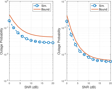
(a)                               (b)

Figure 3: Outage probabilities as functions of SNRs with $D=16$ and $T=2$: (a) $M=2$; (b) $M=1$.

The impact of $M$ and $T$ on the outage probability is shown in Fig. 4 when ${\sf SNR}=6$ dB. Since $M$ is the number of interfering signals, the outage probability increases with $M$ as shown in Fig. 4 (a). In Fig. 4 (b), as expected, the outage probability increases with $T$. Furthermore, since the bound is tight, we can choose $T$ for a sufficiently low target outage probability. Note that the first term on the RHS in (27) in Fig. 4 (b) is not an upper-bound when $T$ is large (e.g., $T\geq 8$). When $T=10$, the 2nd term on the RHS in (27) becomes 0.6727, which is not negligible. As shown in Fig. 4 (b), the 2nd term needs to be taken into account for the upper-bound when $T$ is not small. However, since we are mainly interested in a low outage probability (e.g., $\leq 10^{-3}$), the impact of the 2nd term on the upper-bound is negligible.

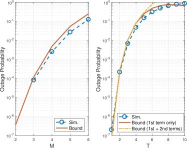
(a)                               (b)

Figure 4: Outage probabilities as functions of $M$ and $T$ when ${\sf SNR}=6$ dB: (a) outage probability versus $M$ with $D=32$ and $T=4$; (b) outage probability versus $T$ with $D=16$ and $M=2$.

Fig. 5 shows the outage probability as a function of $D$ when $M=3$, ${\sf SNR}=6$ dB, and $T\in\{2,4\}$. Clearly, a better performance is achieved with $D$ due to a higher diversity gain. It is shown that as long as $d$ is sufficiently large (due to a large $D$ or small $T$), the bound with the first term in (27) is reasonably tight and can be used to predict the performance in terms of the outage probability.

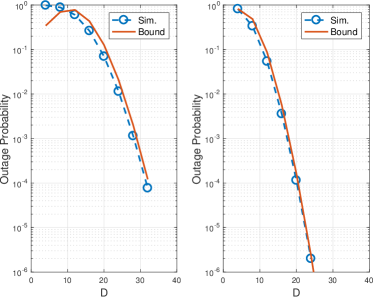
(a)                               (b)

Figure 5: Outage probabilities as a function of $D$ with $M=3$ and ${\sf SNR}=6$ dB: (a) $T=4$; (b) $T=2$.

V-B Average Error Probability for Finite-Length Codes

As mentioned earlier, a careful determination of $T_{k}$ or $R_{k}$ is necessary to keep the outage probability low (for successful SIC). If finite-length codes are used, we need to consider the average error probability instead of the outage probability. In this subsection, we consider the average error probability in (48).

In Fig. 6, we consider a repetition-based NOMA system with $B=3$ and $n=512$ (bits). It is assumed that one user in layer 1 (transmitting $L$ copies), two users in layer 2 (each user transmitting $L/2$ copies), and four users in layer 3 (each user transmitting $L/4$ copies). The average error probability in each layer for different values of the code rate, $R$, is shown in Fig. 6 with the bound from (48). As shown in Fig. 6 (a), the signal in layer 1 needs to have $R\leq 0.75$ for an average error probability of $10^{-3}$. It is also possible to decide the code rates for the signals in layers 2 and 3 for an average error probability of $10^{-3}$ using the bound from (48), because the bound is sufficiently tight. In Fig. 6 (b), we can see that the rates increase more than twice when $L=16$ compared with the rates when $L=8$ (which are shown in Fig. 6 (a)) with a target error probability of $10^{-3}$. If the target error probability further decreases, the rate gap increases. This indicates that the repetition-based NOMA scheme can be more efficient with a large $L$ and a low target error probability thanks to a high diversity gain.

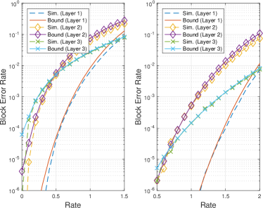
(a)                               (b)

Figure 6: Average error probabilities as a function of $R$ with $B=3$ and ${\sf SNR}=6$ dB: (a) $L=8$; (b) $L=16$.

In Figs. 3 -  6, we consider the instantaneous SINR in (13) for simulations. Since (13) is obtained under the assumption of A1, it would be necessary to consider simulations with interleaved finite-length blocks. To this end, quadrature phase shift keying (QPSK) is considered with a block length of $n/2$ (since one QPSK symbol can transmit 2 bits). Random interleaving at symbol-level is considered. In Fig. 7, we show the average error probability for different values of the code rate when there are $M\in\{2,3\}$ interfering signals, $D=16$, and ${\sf SNR}=6$ dB. It is shown that the average error probability with QPSK is slightly lower than that with the instantaneous SINR in (13). This may result from the fact that the correlation cannot be zero by symbol-level random interleaving and the correlation reduces the interference level.

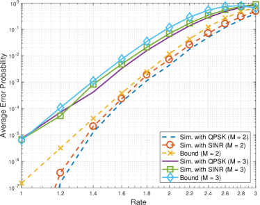
Figure 7: Average error probabilities as a function of $R$ with $D=16$, $n=512$, ${\sf SNR}=6$ dB, and $M\in\{2,3\}$.

To see the impact of the length of finite-length codes, $n$, on the average error probability, we perform simulations and show the results in Fig. 8 when with $D=16$, $M=2$, $R=2$, and ${\sf SNR}=6$ dB. As expected, the average error probability decreases with $n$, while it becomes saturated for a sufficiently large $n$. We can also confirm that the bound in (48) can be used to predict the performance with finite-length codes from Figs. 7 and 8.

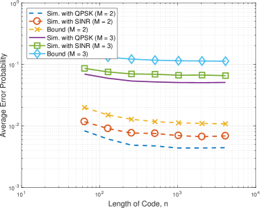
Figure 8: Outage probabilities as a function of $n$ with $D=16$, $M=2$, $R=2$, and ${\sf SNR}=6$ dB.

VI Concluding Remarks

In this paper, we discussed a NOMA scheme based on repetition to exploit high diversity gains. The resulting scheme, called repetition-based NOMA, was able to provide a low error probability without instantaneous CSI-based power allocation thanks to high diversity gains. In order to guarantee a target performance, a closed-form expression for an upper-bound on the outage probability was derived so that key parameters (e.g., the code rate) can be decided accordingly. The case of finite-length codes was also considered with the average error probability. Simulation results demonstrated that the derived upper-bound is reasonably tight and can be used to decide key parameters that meet a certain target performance.

Since we mainly focused on the performance analysis to derive a closed-form expression for the outage probability in terms of key parameters, we did not work on other issues, e.g., scheduler design. The design of scheduler would be an interesting topic to be studied in the future, which might be based on the derived closed-form expression for the outage probability in this paper.

Appendix A Proof of Lemma 1

Since ${\mathbb{E}}[\chi_{2n}^{2}]=2n$ and ${\rm Var}(\chi_{2n}^{2})=4n$, it can be shown that

$${\mathbb{E}}[\Omega^{2}]=\frac{1}{N^{2}}\left(4M^{2}N^{2}+4NM\right)=4M\left(M+\frac{1}{N}\right).$$ (49)

The 2nd moment of $W$ is given by

$${\mathbb{E}}[W^{2}] ={\mathbb{E}}\left[\sum_{l=1}^{D}\sum_{l^{\prime}=1}^{D}\alpha_{l}\alpha_{l^{\prime}}Y_{l}Y_{l^{\prime}}\right]$$ (50)

$$=\sum_{l=1}^{D}{\mathbb{E}}[\alpha_{l}^{2}]{\mathbb{E}}[Y_{l}^{2}]+\sum_{l\neq l^{\prime}}{\mathbb{E}}[\alpha_{l}\alpha_{l^{\prime}}]{\mathbb{E}}[Y_{l}]{\mathbb{E}}[Y_{l^{\prime}}]$$ (51)

$$=D\alpha_{(2)}(4M+4M^{2})+4M^{2}D(D-1)\sigma_{1,2},$$ (52)

where $\alpha_{(2)}={\mathbb{E}}[\alpha_{l}^{2}]$ and $\sigma_{1,2}={\mathbb{E}}[\alpha_{1}\alpha_{2}]$. Since $X_{l,k}$ is an exponential random variable under the assumption of A2, $\alpha_{l}$ is expressed as $\alpha_{l}=\frac{D_{l}}{\sum_{l^{\prime}=1}^{D}D_{l^{\prime}}}$, where $D_{l}\sim{\rm Exp}(1)$ is an independent exponential random variable with parameter 1. The distribution of $\alpha_{l}$ is the same as that of the minimum of $D-1$ independent standard uniform random variables [23, Example 4.6], i.e., $f(\alpha_{l})=(D-1)(1-\alpha_{l})^{D-2}$, $\alpha_{l}\in[0,1]$. Thus, we have

$$\alpha_{(2)}=\frac{2}{D(D+1)}.$$ (53)

In addition, the distribution of $\alpha_{1}+\alpha_{2}=\frac{D_{1}+D_{2}}{\sum_{l=1}^{D}D_{l}}$ is the same as the distribution of the 2nd smallest order statistic among $D-1$ independent standard uniform random variables. From this, since

$${\mathbb{E}}[(\alpha_{1}+\alpha_{2})^{2}]={\mathbb{E}}[\alpha_{1}^{2}]+{\mathbb{E}}[\alpha_{2}^{2}]+2{\mathbb{E}}[\alpha_{1}\alpha_{2}],$$

we have

$${\mathbb{E}}[\alpha_{1}\alpha_{2}] =\frac{{\mathbb{E}}[(\alpha_{1}+\alpha_{2})^{2}]}{2}-{\mathbb{E}}[\alpha_{1}^{2}]$$ (54)

$$=\frac{6}{2D(D+1)}-\frac{2}{D(D+1)}=\frac{1}{D(D+1)},$$ (55)

because the 2nd moment of the 2nd smallest order statistic is $\frac{6}{D(D+1)}$ [23, Eq. (8.4)]. Then, it can be shown that

$${\mathbb{E}}[W^{2}]=\frac{2}{D+1}(4M+4M^{2})+\frac{D-1}{D+1}4M^{2}.$$ (56)

Consequently, from (49) and (56) we can find that the 2nd moments of $W$ and $\Omega$ are the same if $N$ is given as in (22), which completes the proof.

Appendix B Proof of Lemma 2

Using the Chernoff bound [24], it can be shown that

$$\Pr(Z_{D}<z) \leq{\mathbb{E}}[e^{-t(Z_{D}-z)}]$$ (57)

$$=e^{2Dtz}\left(\frac{1}{1+2t}\right)^{D}=\left(\frac{e^{2tz}}{1+2t}\right)^{D}.$$ (58)

Here, $t>0$. Letting $z=\frac{1}{1+2t}$, we have

$$\Pr(Z_{D}<z)\leq(ze^{1-z})^{D},\ z\in[0,1),$$ (59)

which is reasonably tight. For $z>1$, it can also be shown that

$$\Pr(Z_{D}>z)\leq(ze^{1-z})^{D}.$$ (60)

As in [25], the upper-bound in (59) can be tighter using a correction term as follows:

$$\Pr(Z_{D}\leq z) \leq F_{D}(z)$$ (61)

$$=(zc_{D}e^{1-zc_{D}})^{D},\ z\in[0,1/c_{D}],$$ (62)

where $c_{D}$ is the correction term that is given in (18). Thus, if $M=0$, (62) can be applied to (16), which results in (17).

For the case that $M>0$, we need to take into account the interference. In (25), let $Y=\frac{\chi_{2NM}^{2}}{2}$. Then, using (62), it can be shown that

$$\tilde{\mathbb{P}}_{k} =\int_{0}^{\infty}\Pr\left(Z_{D}<\frac{T}{D}\left(\frac{y}{N}+\frac{1}{{\sf SNR}}\right)\right)f_{Y}(y)dy$$ (63)

$$\leq\int_{0}^{\kappa}(c_{D}\phi(y)e^{1-c_{D}\phi(y)})^{D}f_{Y}(y)dy+\int_{\kappa}^{\infty}f_{Y}(y)dy$$ (64)

$$\leq\int_{0}^{\infty}(c_{D}\phi(y)e^{1-c_{D}\phi(y)})^{D}f_{Y}(y)dy+\int_{\kappa}^{\infty}f_{Y}(y)dy,\quad$$ (65)

where $f_{Y}(y)$ represents the pdf of $Y$ and

$$\phi(y)=\frac{T}{D}\left(\frac{y}{N}+\frac{1}{{\sf SNR}}\right)\ \mbox{and}\ \kappa=N\left(\frac{D}{c_{D}T}-\frac{1}{{\sf SNR}}\right).$$

The first term on the RHS in (65) can be expressed as

$$\psi =\left(\frac{c_{D}eT}{D}\right)^{D}e^{-\frac{c_{D}T}{{\sf SNR}}}$$ (66)

$$\ \times\int_{0}^{\infty}\left(\frac{y}{N}+\frac{1}{{\sf SNR}}\right)^{D}e^{-\frac{c_{D}T}{N}y}f_{Y}(y)dy$$ (67)

$$=\frac{1}{D!}\left(\frac{T}{{\sf SNR}}\right)^{D}e^{-\frac{c_{D}T}{{\sf SNR}}}$$ (68)

$$\ \times\sum_{n=0}^{D}\binom{D}{n}\left(\frac{{\sf SNR}}{N}\right)^{n}\int_{0}^{\infty}e^{-\frac{c_{D}T}{N}y}\frac{y^{MN-1+n}e^{-y}}{(MN-1)!}dy$$ (69)

$$=\frac{1}{D!}\left(\frac{T}{{\sf SNR}}\right)^{D}e^{-\frac{c_{D}T}{{\sf SNR}}}$$ (70)

$$\ \times\sum_{n=0}^{D}\binom{D}{n}\left(\frac{{\sf SNR}}{N}\right)^{n}\left(\frac{1}{1+\frac{c_{D}T}{N}}\right)^{MN+n}\frac{(MN+n-1)!}{(MN-1)!}$$ (71)

$$=\frac{1}{D!}\left(\frac{T}{{\sf SNR}}\right)^{D}\frac{e^{-\frac{c_{D}T}{{\sf SNR}}}}{(1+\frac{c_{D}T}{N})^{MN}}$$ (72)

$$\ \times\sum_{n=0}^{D}\binom{D}{n}\left(\frac{{\sf SNR}}{N+c_{D}T}\right)^{n}\frac{(MN+n-1)!}{(MN-1)!},$$ (73)

which becomes (29).

From (60), the 2nd term on the RHS in (65) is bounded as follows:

$$\Pr(Y\geq\kappa) =\Pr\left(\frac{\chi_{2NM}^{2}}{2NM}\geq\frac{1}{M}\left(\frac{D}{c_{D}T}-\frac{1}{{\sf SNR}}\right)\right)$$ (74)

$$\leq\left(\frac{d}{M}e^{1-\frac{d}{M}}\right)^{NM}=\left(\frac{de}{M}\right)^{NM}e^{-dN},$$ (75)

which is the 2nd term on the RHS in (27). This completes the proof.

Appendix C Proof of Lemma 3

Using the inequality of arithmetic and geometric means, it can be shown that

$$\prod_{t=0}^{n-1}(MN+t)\leq\left(MN+\frac{\sum_{t=0}^{n-1}t}{n}\right)^{n}=\left(MN+\frac{n-1}{2}\right)^{n}.$$ (76)

In (29), since $n\leq D$, using (76), it follows

$$\sum_{n=0}^{D}\binom{D}{n}\left(\frac{{\sf SNR}}{N+c_{D}T}\right)^{n}\prod_{t=0}^{n-1}(MN+t)$$ (77)

$$\leq\left(1+\frac{{\sf SNR}}{N+c_{D}T}\left(MN+\frac{D-1}{2}\right)\right)^{D}.$$ (78)

Substituting (78) into (29), with $N=\frac{D+1}{2}$, we have

$$\psi \leq\frac{e^{-\frac{c_{D}T}{{\sf SNR}}}}{D!}\left(\frac{T}{{\sf SNR}}\right)^{D}\left(1+\frac{c_{D}T}{N}\right)^{-MN}$$ (79)

$$\ \times\left(1+\frac{{\sf SNR}}{N+c_{D}T}\left(MN+\frac{D-1}{2}\right)\right)^{D}$$ (80)

$$\leq\frac{(1+\frac{c_{D}T}{N})^{-\frac{M}{2}}}{D!}\nu^{D},$$ (81)

where $\nu=\frac{T}{{\sf SNR}}\left(1+\frac{2c_{D}T}{D+1}\right)^{-\frac{M}{2}}\left(1+\frac{{\sf SNR}(D(M+1)+M-1)}{D+1+2c_{D}T}\right)$. In (81), the last inequality is due to the fact that $e^{-\frac{c_{D}T}{{\sf SNR}}}\leq 1$. Then, we can see that $\nu<1$ if (31) holds.

From (26), we have

$$c_{D}T=\frac{D{\sf SNR}}{d{\sf SNR}+1}\approx\frac{D}{d},\ {\sf SNR}\gg 1.$$ (82)

To determine $C$ in (30), from (82), it can be shown that

$$\frac{1}{1+\frac{c_{D}T}{N}} =\frac{1}{1+\frac{2c_{D}T}{D+1}}=\frac{1}{1+\frac{2D{\sf SNR}}{(D+1)(d{\sf SNR}+1)}}$$ (83)

$$\leq\frac{1}{1+\frac{{\sf SNR}}{d{\sf SNR}+1}}=\frac{1+d{\sf SNR}}{1+(1+d){\sf SNR}},$$ (84)

we have $C=\left(\frac{1}{1+\frac{{\sf SNR}}{d{\sf SNR}+1}}\right)^{\frac{M}{2}}\geq\left(\frac{1}{1+\frac{c_{D}T}{N}}\right)^{\frac{M}{2}}$, where $C$ is independent of $D$.

Appendix D Proof of Lemma 4

As ${\sf SNR}\to\infty$, from (73), after some manipulations, we can show that

$$\bar{\psi} =\left(\frac{c_{D}eT}{D}\right)^{D}\int_{0}^{\infty}\left(\frac{y}{N}\right)^{D}e^{-\frac{c_{D}T}{N}y}f_{Y}(y)dy$$ (85)

$$=\left(\frac{c_{D}eT}{DN}\right)^{D}\frac{\Gamma(MN+D)}{\Gamma(MN)}\frac{1}{\left(1+\frac{c_{D}T}{N}\right)^{MN+D}}$$ (86)

$$=\frac{1}{D!}\frac{\Gamma(MN+D)}{\Gamma(MN)}\left(\frac{T}{N+c_{D}T}\right)^{D}\frac{1}{\left(1+\frac{c_{D}T}{N}\right)^{MN}}$$ (87)

$$=\binom{MN+D-1}{MN-1}\left(\frac{T}{N+c_{D}T}\right)^{D}\left(\frac{N}{N+c_{D}T}\right)^{MN},$$ (88)

which becomes (33).

References

- [1] Z. Ding, Y. Liu, J. Choi, M. Elkashlan, C. L. I, and H. V. Poor, “Application of non-orthogonal multiple access in LTE and 5G networks,” IEEE Communications Magazine, vol. 55, pp. 185–191, February 2017.
- [2] J. Choi, “NOMA: Principles and recent results,” in 2017 International Symposium on Wireless Communication Systems (ISWCS), pp. 349–354, Aug 2017.
- [3] Y. Liu, M. Elkashlan, Z. Ding, and G. K. Karagiannidis, “Fairness of user clustering in MIMO non-orthogonal multiple access systems,” IEEE Communications Letters, vol. 20, pp. 1465–1468, July 2016.
- [4] J. Choi, “On generalized downlink beamforming with NOMA,” J. Communications and Networks, vol. 19, pp. 319–328, August 2017.
- [5] J. Seo and Y. Sung, “Beam design and user scheduling for nonorthogonal multiple access with multiple antennas based on Pareto optimality,” IEEE Trans. Signal Processing, vol. 66, pp. 2876–2891, June 2018.
- [6] Y. Liang, X. Li, J. Zhang, and Z. Ding, “Non-orthogonal random access for 5G networks,” IEEE Trans. Wireless Communications, vol. 16, pp. 4817–4831, July 2017.
- [7] J. Choi, “NOMA-based random access with multichannel ALOHA,” IEEE J. Selected Areas in Communications, vol. 35, pp. 2736–2743, Dec 2017.
- [8] C. Bockelmann, N. Pratas, H. Nikopour, K. Au, T. Svensson, C. Stefanovic, P. Popovski, and A. Dekorsy, “Massive machine-type communications in 5G: physical and MAC-layer solutions,” IEEE Communications Magazine, vol. 54, pp. 59–65, September 2016.
- [9] N. Zhang, J. Wang, G. Kang, and Y. Liu, “Uplink nonorthogonal multiple access in 5G systems,” IEEE Communications Letters, vol. 20, pp. 458–461, March 2016.
- [10] J. Choi, “Joint rate and power allocation for NOMA with statistical CSI,” IEEE Trans. Communications, vol. 65, pp. 4519–4528, Oct 2017.
- [11] P. Xu, Y. Yuan, Z. Ding, X. Dai, and R. Schober, “On the outage performance of non-orthogonal multiple access with 1-bit feedback,” IEEE Trans. Wireless Communications, vol. 15, pp. 6716–6730, Oct 2016.
- [12] J. Choi, “Performance analysis for transmit antenna diversity with/without channel information,” IEEE Trans. Veh. Technol., vol. 51, pp. 101–113, Jan. 2002.
- [13] Y. Polyanskiy, H. V. Poor, and S. Verdu, “Channel coding rate in the finite blocklength regime,” IEEE Trans. Information Theory, vol. 56, pp. 2307–2359, May 2010.
- [14] D. Malak, H. Huang, and J. G. Andrews, “Throughput maximization for delay-sensitive random access communication,” IEEE Trans. Wireless Communications, vol. 18, pp. 709–723, Jan 2019.
- [15] D. Tse and P. Viswanath, Fundamentals of Wireless Communication. Cambridge University Press, 2005.
- [16] M. Chiang, P. Hande, T. Lan, and C. W. Tan, Power Control in Wireless Cellular Networks. Foundations and Trends in Networking, Now Publisher Inc., 2008.
- [17] E. Biglieri, Coding for Wireless Channels. New York: Springer, 2005.
- [18] J. Choi, Optimal Combining and Detection. Cambridge University Press, 2010.
- [19] D. J. C. MacKay, Information Theory, Inference, and Learning Algorithms. Cambridge University Press, 2003.
- [20] V. Y. F. Tan and M. Tomamichel, “The third-order term in the normal approximation for the AWGN channel,” IEEE Trans. Information Theory, vol. 61, pp. 2430–2438, May 2015.
- [21] G. Durisi, T. Koch, and P. Popovski, “Toward massive, ultrareliable, and low-latency wireless communication with short packets,” Proceedings of the IEEE, vol. 104, pp. 1711–1726, Sept 2016.
- [22] S. Verdu, Multiuser Detection. Cambridge University Press, 1998.
- [23] M. Ahsanullah, V. Nevzorov, and M. Shakil, An Introduction to Order Statistics. Atlantis Studies in Probability and Statistics, Atlantis Press, 2013.
- [24] M. Mitzenmacher and E. Upfal, Probability and Computing: Randomized Algorithms and Probability Analysis. Cambridge University Press, 2005.
- [25] J. Choi, “On error rate analysis for URLLC over multiple fading channels,” in Proc. IEEE WCNC, pp. 1–5, Apr. 2020.