Abstract

We study the potential of future Electron-Ion Collider (EIC) data to probe four-fermion operators in the Standard Model Effective Field Theory (SMEFT). The ability to perform measurements with both polarized electron and proton beams at the EIC provides a powerful tool that can disentangle the effects from different SMEFT operators. We compare the potential constraints from an EIC with those obtained from Drell-Yan data at the Large Hadron Collider. We show that EIC data plays an important complementary role since it probes combinations of Wilson coefficients not accessible through available Drell-Yan measurements.

1 Introduction

The Standard Model (SM) of particle physics has so far been successful in describing all observed laboratory phenomena. No new particles beyond those present in the SM have been discovered at the Large Hadron Collider (LHC) or in other experiments, and no appreciable deviation from SM predictions has been conclusively observed. Given this situation it is increasingly important to understand how indirect signatures of new physics can be probed and constrained by the available data. This effort will help guide future searches for new physics by suggesting in what channels measurable deviations from SM predictions may occur given the current bounds.

A convenient theoretical framework for investigating indirect signatures of heavy new physics without associated new particles is the SM effective field theory (SMEFT) containing higher-dimensional operators formed from SM fields. The leading dimension-6 operator basis of SMEFT for on-shell fields has been completely classified [1, 2] (there is a dimension-5 operator that violates lepton number which we do not consider here). Considerable effort has been devoted to performing global analyses of the availabe data within the SMEFT framework [3, 4, 5, 6, 7, 8, 9, 10, 11, 12, 13, 14]. There are numerous questions that must be addressed when performing global fits within the dimension-6 SMEFT framework, including the need for higher-order corrections in the SM coupling constants [15], the importance of effects from dimension-8 and beyond [16, 17, 18, 19, 20], and the estimation of theoretical errors [21].

Another issue that arises in global fits to the SMEFT parameter space is the appearance of flat directions that occur when the available experimental measurements cannot disentangle the contributions from different Wilson coefficients. These flat directions may be either exact or approximate. There are many examples of this phenomenon. For example, it is well known that Higgs cross section measurements alone cannot distinguish between new-physics corrections to the Higgs couplings to gluons and top quarks [22]. Our focus here will be on 2-lepton, 2-quark four-fermion operators appearing in the SMEFT. The presence of operator combinations not probed by the available low-energy data has been discussed in the literature [23]. The expectation is that these operators are well-probed by high invariant-mass Drell-Yan distributions at the LHC, which has both large integrated luminosity and the requisite high energy for which we expect potential SMEFT corrections to become important. There have indeed been numerous studies of the importance of Drell-Yan measurements in constraining four-fermion operators [23, 24]. However, only a few combinations of Wilson coefficients can be probed in principle by Drell-Yan measurements, a point made previously in the literature [25]. In practice only a subset of even these combinations can be probed due to the nature of the current experimental studies, as we discuss later. Future analyses of constraints on SMEFT operators will need to identify new data sets that measure the combinations not determined by Drell-Yan production at the LHC, such as flavor observables where one-loop effects can help break degeneracies [26, 27].

Our goal in this manuscript is to illustrate the important role that future polarized deep-inelastic scattering (DIS) experiments may play in the study of SMEFT, and in particular in disentangling the effects of four-fermion operators indistinguishable at the LHC. In the coming decade the construction of an electron-ion collider (EIC) with polarization of both electron and proton beams is expected, and high-precision polarized electron-proton data will become available. Some studies of new physics searches possible with an EIC have been performed [28]. However, we are aware of no detailed investigation of what aspects of the SMEFT may be probed at an EIC, and in particular its usefulness in studying combinations of Wilson coefficients not accessible at the LHC. In this paper we consider the following points.

• We study the deviations induced by dimension-6 four-fermion operators in the SMEFT on both polarized and unpolarized charged-current and neutral-current DIS. We determine which regions of parameter space are sensitive to dimension-6 Wilson coefficients. We show that the deviations allowed by current constraints are larger than the current parton distribution function (PDF) errors for both polarized and unpolarized protons. Since the SM DIS hard-scattering cross sections are known through next-to-next-to-leading order in QCD [29, 30], theoretical errors should not be a limiting factor in studies of the SMEFT at an EIC.

• We review the contributions of dimension-6 SMEFT operators to neutral-current Drell-Yan at the LHC, and analytically demonstrate the appearance of approximate flat directions in the space of Wilson coefficients. We show the current experimental measurements at the LHC are not well-suited to SMEFT studies. High invariant-mass forward-backward asymmetry measurements would allow additional probes of the SMEFT parameter space, a point also emphasized in Ref. [25]. However, even with such observables many combinations of Wilson coefficients remain poorly tested in LHC Drell-Yan production and would benefit from polarized DIS measurements.

• We perform fits to Drell-Yan data from the LHC to numerically illustrate the flat directions. We identify several example choices of Wilson coefficients that demonstrate the types of degeneracies that appear at the LHC. We show how data from a future EIC is complementary to that obtained from the LHC and can better probe certin combinations of Wilson coefficients. Combined fits of LHC and projected EIC data lead to much stronger constraints than either experiment alone. We show that the ability to polarize both electron and proton beams at an EIC is crucial in obtaining these projected bounds.

Our paper is organized as follows. We review the aspects of the four-fermion operators in the SMEFT relevant to our analysis in Section 2. In Section 3 we present the formulae needed for the study of unpolarized and polarized DIS. We study the phenomenology of SMEFT contributions to DIS at an EIC in Section 4. We study neutral-current Drell-Yan production of lepton pairs at the LHC in Section 5, where we also demonstrate the appearance of flat directions in the space of Wilson coefficients. In Section 6 we present the main results of our paper, fits to the LHC and projected EIC data for a range of different scenarios. We emphasize the complementarity of the two experiments, and show the importance of polarized measurements at the EIC. Finally, we conclude in Section 7.

2 Review of the SMEFT

We review in this section aspects of the SMEFT relevant for our analysis of DIS and Drell-Yan. The SMEFT is an extension of the SM Lagrangian to include terms suppressed by an energy scale $\Lambda$ at which the ultraviolet completion becomes important and new particles beyond the SM appear. Truncating the expansion in $1/\Lambda$ at dimension-6, and ignoring operators of odd-dimension which violate lepton number, we have

$${\cal L}={\cal L}_{SM}+\sum_{i}C_{i}{\cal O}_{i}+\ldots,$$ (1)

where the ellipsis denotes operators of higher dimensions. The Wilson coefficients defined above have dimensions of $1/\Lambda^{2}$. When computing cross sections we consider only the leading interference of the SM amplitude with the dimension-6 contribution. This is consistent with our truncation of the SMEFT expansion above, since the dimension-6 squared contributions are formally the same order in the $1/\Lambda$ expansion as the dimension-8 terms which we neglect. The following four-fermion operators in Table 1 can affect both DIS and Drell-Yan at leading-order in the coupling constants for massless fermions, which we assume here.

${\cal O}_{lq}^{(1)}$	$(\bar{l}\gamma^{\mu}l)(\bar{q}\gamma_{\mu}q)$	${\cal O}_{lu}$	$(\bar{l}\gamma^{\mu}l)(\bar{u}\gamma_{\mu}u)$
${\cal O}_{lq}^{(3)}$	$(\bar{l}\gamma^{\mu}\tau^{I}l)(\bar{q}\gamma_{\mu}\tau^{I}lq)$	${\cal O}_{ld}$	$(\bar{l}\gamma^{\mu}l)(\bar{d}\gamma_{\mu}d)$
${\cal O}_{eu}$	$(\bar{e}\gamma^{\mu}e)(\bar{u}\gamma_{\mu}u)$	${\cal O}_{qe}$	$(\bar{q}\gamma^{\mu}q)(\bar{e}\gamma_{\mu}e)$
${\cal O}_{ed}$	$(\bar{e}\gamma^{\mu}e)(\bar{d}\gamma_{\mu}d)$

Table 1: Dimension-6 four-fermion operators contributing to DIS and DY at leading order in the coupling constants.

$q$ and $l$ denote left-handed quark and lepton doublets, while $u$, $d$ and $e$ denote right-handed singlets for the up quarks, down quarks and leptons, respectively. $\tau^{I}$ denote the SU(2) Pauli matrices. We have suppressed flavor indices for these operators, and in our analysis we assume flavor universality for simplicity. We note that the overall electroweak couplings that govern lepton-pair production are also shifted in the SMEFT by operators other than those considered above. Such contributions are far better bounded through other data sets such as precision $Z$-pole observables [24], and we neglect them here. The above assumptions leave us with the seven Wilson coefficients associated with the operators in Table 1 entering the predictions for our cross sections.

3 Review of DIS formalism

We review in this section the relevant formulae describing both unpolarized and polarized DIS in the process $l(k)+P(P)\to l^{\prime}(k^{\prime})+X$, where $P$ denotes a proton. We consider the leading-order partonic process $l(k)+q(p)\to l^{\prime}(k^{\prime})+q_{f}(p_{f})$, including both the SM contributions and the corrections induced by dimension-6 SMEFT operators. Expressions for the charged-current process are also given below. The relation between partonic and hadronic momenta is $p=xP$. It is standard to introduce the momentum transfer $q=k-k^{\prime}$, with $q^{2}=-Q^{2}$. We recall here some of the basic kinematic relations relevant for DIS:

$$p\cdot k=\frac{xs}{2},\;\;p_{f}\cdot k^{\prime}=\frac{xs}{2},\;\;k\cdot k^{\prime}=\frac{Q^{2}}{2},\;\;P\cdot q=\frac{Q^{2}}{2x},\;\;\;p\cdot q=\frac{Q^{2}}{2},\;\;\frac{P\cdot q}{P\cdot k}=\frac{p\cdot q}{p\cdot k}=y.$$ (2)

We can use these relations to show that $Q^{2}=xys$ at leading-order.

The matrix elements receive SM contributions from both photon and $Z$-boson exchange. In the SMEFT there is an additional correction from four-fermion contact interactions. We can split the differential cross section into the following contributions that arise from the interference of the relevant diagrams:

$$\frac{d^{2}\sigma}{dx\,dQ^{2}}=\frac{4\pi\alpha^{2}}{xQ^{4}}\sum_{q}f_{q,\lambda_{q}}(x,Q^{2})\left\{\frac{d^{2}\sigma^{\gamma\gamma}}{dxdQ^{2}}+\frac{d^{2}\sigma^{\gamma Z}}{dxdQ^{2}}+\frac{d^{2}\sigma^{ZZ}}{dxdQ^{2}}+\frac{d^{2}\sigma^{\gamma SMEFT}}{dxdQ^{2}}+\frac{d^{2}\sigma^{ZSMEFT}}{dxdQ^{2}}\right\}.$$ (3)

We have used $\lambda_{e}$ and $\lambda_{q}$ to respectively denote the helicities of the lepton and quark that enter the hard-scattering process. For fully-polarized states, $\lambda_{i}=\pm 1$ in our normalization. The leading-order expressions for the SM contributions are given below:

$$\frac{d^{2}\sigma^{\gamma\gamma}}{dxdQ^{2}} = xQ_{q}^{2}\left[(1-y)+\frac{y^{2}}{2}+\frac{\lambda_{q}\lambda_{e}}{2}y(2-y)\right],$$

$$\frac{d^{2}\sigma^{\gamma Z}}{dxdQ^{2}} = x\frac{e_{q}N_{\gamma Z}}{2}\left[g_{L}^{q}g_{L}^{e}(1-\lambda_{q})(1-\lambda_{e})+g_{R}^{q}g_{R}^{e}(1+\lambda_{q})(1+\lambda_{e})\right.$$

$$\left.+g_{R}^{q}g_{L}^{e}(1-y)^{2}(1+\lambda_{q})(1-\lambda_{e})+g_{L}^{q}g_{R}^{e}(1-y)^{2}(1-\lambda_{q})(1+\lambda_{e})\right],$$

$$\frac{d^{2}\sigma^{ZZ}}{dxdQ^{2}} = x\frac{N_{ZZ}}{4}\left[(g_{L}^{q}g_{L}^{e})^{2}(1-\lambda_{q})(1-\lambda_{e})+(g_{R}^{q}g_{R}^{e})^{2}(1+\lambda_{q})(1+\lambda_{e})\right.$$ (4)

$$\left.+(g_{R}^{q}g_{L}^{e})^{2}(1-y)^{2}(1+\lambda_{q})(1-\lambda_{e})+(g_{L}^{q}g_{R}^{e})^{2}(1-y)^{2}(1-\lambda_{q})(1+\lambda_{e})\right].$$

We have introduced the following abbreviations in these expressions:

$$N_{\gamma Z}=\frac{G_{F}M_{Z}^{2}}{2\sqrt{2}\pi\alpha}\frac{Q^{2}}{Q^{2}+M_{Z}^{2}},\;\;\;N_{ZZ}=N_{\gamma Z}^{2}.$$ (5)

For the SM left-handed and right-handed fermion couplings we follow the conventions of Ref. [31]:

$$g_{L}^{f}=I_{3}^{f}-Q_{f}s_{W}^{2},\;\;\;g_{R}^{f}=-Q_{f}s_{W}^{2}.$$ (6)

We give below the expressions for the SMEFT corrections in the up-quark initial state:

$$\frac{d^{2}\sigma_{u}^{\gamma SMEFT}}{dxdQ^{2}} = -x\frac{Q_{u}Q^{2}}{8\pi\alpha}\left[C_{eu}(1+\lambda_{u})(1+\lambda_{e})+(C_{lq}^{(1)}-C_{lq}^{(3)})(1-\lambda_{u})(1-\lambda_{e})\right.$$

$$\left.+(1-y)^{2}C_{lu}(1+\lambda_{u})(1-\lambda_{e})+(1-y)^{2}C_{qe}(1-\lambda_{u})(1+\lambda_{e})\right]$$

$$\frac{d^{2}\sigma_{u}^{ZSMEFT}}{dxdQ^{2}} = -x\frac{N_{\gamma Z}Q^{2}}{8\pi\alpha}\left[g_{R}^{u}g_{R}^{e}C_{eu}(1+\lambda_{u})(1+\lambda_{e})+g_{L}^{u}g_{L}^{e}(C_{lq}^{(1)}-C_{lq}^{(3)})(1-\lambda_{u})(1+\lambda_{e})\right.$$ (7)

$$\left.+g_{R}^{u}g_{L}^{e}(1-y)^{2}C_{lu}(1+\lambda_{u})(1-\lambda_{e})+g_{L}^{u}g_{R}^{e}(1-y)^{2}C_{qe}(1-\lambda_{u})(1+\lambda_{e})\right].$$

To obtain results for the down-quark initial state, we simply make the following replacements in the formulae above:

$$Q_{u}\to Q_{d},\;\;g_{L,R}^{u}\to g_{L,R}^{d},\;\;C_{lu}\to C_{ld},\;\;C_{eu}\to C_{ed},\;\;C_{lq}^{(3)}\to-C_{lq}^{(3)}.$$ (8)

From these formulae we can obtain the results for the polarized and unpolarized cross sections. The unpolarized cross section is obtained by averaging over the two quark helicity possibilities $\lambda_{q}=\pm 1$ and setting the PDF in Eq. (3) to the usual unpolarized one, while the polarized result is obtained by taking the difference $\lambda_{q}=-1$ minus $\lambda_{q}=+1$ and interpreting the PDF in Eq. (3) as the usual polarized PDF. Upon forming these two combinations we obtain four physically observable differential cross sections in neutral-current DIS: the polarized and unpolarized cross sections with positive or negative $\lambda_{e}$.

We briefly present here the formulae for the charged-current process $\nu_{\mu}(k)+u(p)\to\mu(k^{\prime})+d(p_{f})$. We directly show the results for the unpolarized and polarized partonic cross sections. The SM differential cross sections are

$$\frac{d\sigma^{WW}_{unpol}}{dxdQ^{2}} = \frac{g^{4}(1-\lambda_{e})}{64\pi(Q^{2}+M_{W}^{2})^{2}},$$

$$\frac{d\Delta\sigma^{WW}}{dxdQ^{2}} = \frac{g^{4}(1-\lambda_{e})}{32\pi(Q^{2}+M_{W}^{2})^{2}}.$$ (9)

The corrections coming from SMEFT four-fermion operators are

$$\frac{d\sigma^{WSMEFT}_{unpol}}{dxdQ^{2}} = -\frac{g^{2}(1-\lambda_{e})C_{lq}^{(3)}}{8\pi(Q^{2}+M_{W}^{2})},$$

$$\frac{d\Delta\sigma^{WSMEFT}}{dxdQ^{2}} = -\frac{g^{2}(1-\lambda_{e})C_{lq}^{(3)}}{4\pi(Q^{2}+M_{W}^{2})}.$$ (10)

We note that only the left-handed polarization state contributes.

4 Phenomenology of DIS at the EIC

In this section we briefly review the expected parameters of an EIC, and study the deviations induced by the four-fermion SMEFT operators considered above on both neutral and charged-current DIS. The recently announced EIC at Brookhaven National Laboratory will be a high-energy and high-luminosity tool to investigate the structure of nucleons and nuclei. The physics potential of the EIC is detailed in Ref. [28], as are the various machine parameters assumed below in our study. It is planned to be tunable over a large range of energies, different polarizations and types of heavy ions, as well as protons. The machine is projected to operate at a center-of-mass-energy approaching $\sqrt{s}\approx 140\;\textrm{GeV}$, which we assume in our study. We assume that it will collect $10\,\textrm{fb}^{-1}$, which we split equally among the four modes identified in the previous section (polarized and unpolarized with both positive and negative $\lambda_{e}$). We also study the impact of accumulating $100\,\textrm{fb}^{-1}$. We assume that the EIC will reach 70% polarization for both proton and electron beams.

4.1 Standard Model Contributions

We begin by briefly summarizing and discussing the Standard Model predictions for the different cross sections that will be measured at the future EIC. The expressions in Eq. (4) are evaluated with the electroweak input parameters [32]:

$$\alpha^{-1} =137.036,\;\;\;G_{F}=1.16638\times 10^{-5}\,\textrm{GeV}^{-2},$$

$$M_{Z} =91.1876\,\textrm{GeV},\;\;\;M_{W}=80.379\,\textrm{GeV}.$$ (11)

We use the NNPDF3.1 NLO [33] PDFs in the unpolarized case and NNPDFPol1.1 [34] in the polarized case throughout. We constrain the angular variable $y$, defined in Eq. (2), to be between $0.1$ and $0.9$ for both the neutral and charged current processes, in accordance with values quoted in the literature [36, 35]. To avoid non-perturbative QCD effects impacting our analysis we only consider values of $Q^{2}$ above $(12\;\textrm{GeV})^{2}$. The momentum fraction $x$ is constrained in our fits to be below $0.2$. To provide some intuition regarding the expected evant rates at the EIC we show the SM cross sections for both charged and neutral current processes in Fig. 1.

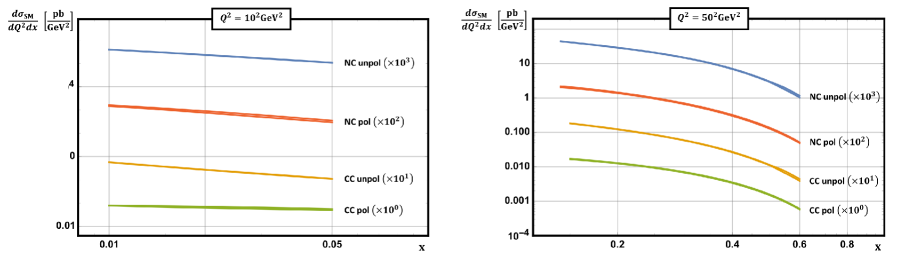
Figure 1: Comparison of unpolarized and polarized Standard Model cross sections for neutral and charged current processes for different values of $Q^{2}$. The cross sections assume $\lambda_{e}=-0.7$. The $1-\sigma$ error band stems from the uncertainty of the corresponding PDFs.

4.2 SMEFT Contributions

We next allow for SMEFT four-fermion operator contributions to modify our observables. We assume $C_{i}=1/\textrm{TeV}^{2}$ in order to illustrate these effects. First we illustrate the potential of the DIS observables by plotting the expected relative deviation from the Standard Model over a large part of $(x,Q^{2})$ space in Fig. 2 for two example Wilson coefficients. We see that the deviations grow with both $x$ and $Q^{2}$, indicating that these phase-space regions will be most sensitive to the SMEFT effects. It is evident from these plots that PDF uncertainties are sub-dominant to potential SMEFT deviations, even in the case of a polarized proton beam. We also note that the expected deviations become large relative to the expected precision of the EIC.

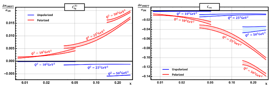
Figure 2: Neutral-current SMEFT deviation normalized to Standard Model predictions for the Wilson coefficients $C_{lq}^{(1)}$ and $C_{eu}$ as a function of Bjorken-$x$ for different choices of $Q^{2}$. The error bands illustrate the the $1-\sigma$ interval stemming from the uncertainty of the PDFs. The SMEFT deviations for the unpolarized cross section are in blue, and for the polarized cross section in red. We note that the kinematic constraint on $y$ leads to the turn-on of the curves at different $x$-values for each $Q^{2}$ choice.

We now show how different observables are sensitive to different combinations of Wilson coefficients. This is illustrated in Fig. 3, where we compare the relative deviations for each of the Wilson coefficients switched on separately for different electron polarizations. We see that for positive electron polarization we primarily probe $C_{qe}$ and $C_{eu}$, while $C_{lq}^{(1)}$ and $C_{lq}^{(3)}$ only lead to a small shift of the cross section. For negative electron polarization we find the opposite behavior. We will see later that this ability of the EIC to discriminate between different Wilson coefficients using polarized observables can help probe SMEFT effects difficult to see at the LHC.

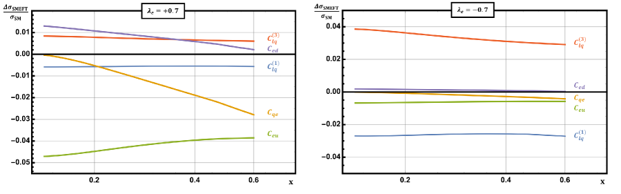
Figure 3: Comparison of the size of the unpolarized SMEFT deviations for each of the Wilson coefficients $C_{qe}$, $C_{eu}$, $C_{ed}$, $C_{lq}^{(1)}$ and $C_{lq}^{(3)}$ for different values of the electron polarization. The plots are for fixed $Q^{2}=(50\,\textrm{GeV})^{2}$.

5 Neutral-current Drell-Yan in the SMEFT

We discuss here the Drell-Yan process at the LHC. Our analysis is performed at leading order in the SMEFT. A partial calculation of the higher-order terms is given in Ref. [24]. Our major focus will be on identifying combinations of Wilson coefficients for which the SMEFT-induced corrections vanish. This shows that the LHC is not sensitive to these combinations, making potential EIC probes important. We will define four example choices of Wilson coefficients that allow us to compare the sensitivities of the LHC and a future EIC in different scenarios.

5.1 Review of Drell-Yan formulae

We first present formulae for the partonic channel $u(p_{1})\bar{u}(p_{2})\to l(p_{3})\bar{l}(p_{4})$. Three diagrams contribute to this process: photon exchange, $Z$-boson exchange, and a four-fermion contact interaction. It is straightforward to derive the differential cross section for this process. We split it into the following contributions, labeled by which diagrammatic interference they arise from:

$$\frac{d\sigma_{u\bar{u}}}{dM^{2}dYdc_{\theta}} = \frac{1}{32\pi M^{2}s}f_{u}(x_{1})f_{\bar{u}}(x_{2})\left\{\frac{d\hat{\sigma}^{\gamma\gamma}_{u\bar{u}}}{dM^{2}dYdc_{\theta}}+\frac{d\hat{\sigma}^{\gamma Z}_{u\bar{u}}}{dM^{2}dYdc_{\theta}}+\frac{d\hat{\sigma}^{ZZ}_{u\bar{u}}}{dM^{2}dYdc_{\theta}}\right.$$ (12)

$$+ \left.\frac{d\hat{\sigma}^{\gamma SMEFT}_{u\bar{u}}}{dM^{2}dYdc_{\theta}}+\frac{d\hat{\sigma}^{ZSMEFT}_{u\bar{u}}}{dM^{2}dYdc_{\theta}}\right\}.$$

Here, $x_{1}$ and $x_{2}$ are the Bjorken momentum fractions of the partons from each proton, $M^{2}$ and $Y$ are respectively the invariant mass and rapidity of the di-lepton system, and $c_{\theta}$ is the cosine of the CM-frame scattering angle of the negatively-charged lepton. To obtain the full hadronic cross section from this partonic channel we integrate this over $x_{1}$ and $x_{2}$. The separate contributions from each diagrammatic interference are given below:

$$\frac{d\hat{\sigma}^{\gamma\gamma}_{u\bar{u}}}{dM^{2}dYdc_{\theta}} = \frac{32\pi^{2}\alpha^{2}Q_{u}^{2}}{3}\frac{\hat{t}^{2}+\hat{u}^{2}}{\hat{s}^{2}},$$

$$\frac{d\hat{\sigma}^{\gamma Z}_{u\bar{u}}}{dM^{2}dYdc_{\theta}} = -\frac{8\pi\alpha Q_{u}g_{Z}^{2}}{3}\frac{(g_{R}^{u}g_{L}^{e}+g_{R}^{e}g_{L}^{u})\hat{t}^{2}+(g_{R}^{u}g_{R}^{e}+g_{L}^{e}g_{L}^{u})\hat{u}^{2}}{\hat{s}(\hat{s}-M_{Z}^{2})},$$

$$\frac{d\hat{\sigma}^{ZZ}_{u\bar{u}}}{dM^{2}dYdc_{\theta}} = \frac{g_{Z}^{4}}{3}\frac{((g_{R}^{u}g_{L}^{e})^{2}+(g_{R}^{e}g_{L}^{u})^{2})\hat{t}^{2}+((g_{R}^{u}g_{R}^{e})^{2}+(g_{L}^{e}g_{L}^{u})^{2})\hat{u}^{2}}{(\hat{s}-M_{Z}^{2})^{2}},$$

$$\frac{d\hat{\sigma}^{\gamma SMEFT}_{u\bar{u}}}{dM^{2}dYdc_{\theta}} = -\frac{8\pi\alpha Q_{u}}{3}\frac{(C_{lu}+C_{qe})\hat{t}^{2}+(C_{eu}+C_{lq}^{(1)}-C_{lq}^{(3)})\hat{u}^{2}}{\hat{s}},$$

$$\frac{d\hat{\sigma}^{ZSMEFT}_{u\bar{u}}}{dM^{2}dYdc_{\theta}} = \frac{2g_{Z}^{2}}{3}\frac{(g_{R}^{u}g_{L}^{e}C_{lu}+g_{R}^{e}g_{L}^{u}C_{qe})\hat{t}^{2}+(g_{R}^{u}g_{R}^{e}C_{eu}+g_{L}^{u}g_{L}^{e}C_{lq}^{(1)}-g_{L}^{u}g_{L}^{e}C_{lq}^{(3)})\hat{u}^{2}}{\hat{s}-M_{Z}^{2}}.$$ (13)

We have identified the usual partonic Mandelstam invariants $\hat{s}=(p_{1}+p_{2})^{2}$, $\hat{t}=(p_{1}-p_{3})^{2}$, $\hat{u}=(p_{1}-p_{4})^{2}$. They depend upon the scattering angle $c_{\theta}$ according to

$$\hat{t}=-\frac{\hat{s}}{2}(1-c_{\theta}),\;\;\;\hat{u}=-\frac{\hat{s}}{2}(1+c_{\theta}).$$ (14)

For the SM left-handed and right-handed fermion couplings we follow the conventions of Ref. [31]:

$$g_{L}^{f}=I_{3}^{f}-Q_{f}s_{W}^{2},\;\;\;g_{R}^{f}=-Q_{f}s_{W}^{2}.$$ (15)

We note that we can obtain the partonic channel $\bar{u}(p_{1})u(p_{2})\to l(p_{3})\bar{l}(p_{4})$ by interchanging $\hat{t}\leftrightarrow\hat{u}$. To obtain results for the down-quark initiated process $d(p_{1})\bar{d}(p_{2})\to l(p_{3})\bar{l}(p_{4})$ we make the following changes in Eq. (13):

$$Q_{u}\to Q_{d},\;\;g_{L,R}^{u}\to g_{L,R}^{d},\;\;C_{lu}\to C_{ld},\;\;C_{eu}\to C_{ed},\;\;C_{lq}^{(3)}\to-C_{lq}^{(3)}.$$ (16)

The sign change for $C_{lq}^{(3)}$ is important as it indicates that the down-quark channel probes the orthogonal combination of $C_{lq}^{(1)}$ and $C_{lq}^{(3)}$ compared to the up-quark channel.

5.2 Flat directions in Drell-Yan

The fact that seven Wilson coefficients contribute to the SMEFT correction but fewer kinematic combinations appear in the matrix elements implies that only certain combinations of Wilson coefficients can be probed with Drell-Yan measurements, a point already made in previous work [25]. We can identify the following features from the above formulae.

• The deviations from dimension-6 operators in the SMEFT are expected to be largest at high invariant mass, when $\hat{s}\gg M_{Z}^{2}$. When we make this approximation in the denominator of the $Z-SMEFT$ interference in Eq. (13), we find that only two combinations of Wilson coefficients proportional to $\hat{t}^{2}$ and $\hat{u}^{2}$ respectively contribute. In the up-quark channel the following combinations appear:

  $$-\frac{8\pi\alpha Q_{u}}{3}\left[(C_{lu}+C_{qe})\right]+\frac{2g_{Z}^{2}}{3}\left[g_{R}^{u}g_{L}^{e}C_{lu}+g_{R}^{e}g_{L}^{u}C_{qe}\right],$$

  $$-\frac{8\pi\alpha Q_{u}}{3}\left[(C_{eu}+C_{lq}^{(1)}-C_{lq}^{(3)})\right]+\frac{2g_{Z}^{2}}{3}\left[g_{R}^{u}g_{R}^{e}C_{eu}+g_{L}^{u}g_{L}^{e}C_{lq}^{(1)}-g_{L}^{u}g_{L}^{e}C_{lq}^{(3)}\right].$$ (17)

  In the down-quark channel similar combinations with the replacements of Eq. (16) appear. In the high-energy limit only these combinations can be probed.

• In principle these combinations can be separately probed by measurements dependent on the lepton kinematics. We note that measurements of the di-lepton system such as the invariant mass or rapidity do not allow these coefficient combinations to be separately determined. These distributions are obtained by integrating inclusively over $c_{\theta}$, and in the high-energy limit depend on only a single combination of Wilson coefficients. However, another limitation becomes apparent if we express the differential cross section in terms of the CM-frame angle $c_{\theta}$. In the $\hat{s}\gg M_{Z}^{2}$ limit the SMEFT correction to the cross section takes the form

  $$A(g_{i},C_{i})(1+c_{\theta}^{2})+B(g_{i},C_{i})c_{\theta},$$ (18)

  where $g_{i}$ and $C_{i}$ denote the SM couplings and dimension-6 Wilson coefficients respectively. $A(g_{i},C_{i})$ is the same combination of couplings that appears in the di-lepton invariant mass and rapidity distributions, while $B(g_{i},C_{i})$ is a different combination. In order to probe $B$ an experimental measurement must integrate over an asymmetric range of $c_{\theta}$, otherwise the $B$ term will integrate to zero. Existing high-mass differential Drell-Yan measurements that go beyond the di-lepton invariant mass and rapidity distributions, such as Ref. [37], focus on quantities such as $|\Delta\eta_{ll}|$, the absolute value of the pseudorapidity distribution between leptons. We can express this variable in terms of the CM-frame scattering angle as

  $$|\Delta\eta_{ll}|=2\,|{\rm arctanh}(c_{\theta})|.$$ (19)

  Since this variable is symmetric under $c_{\theta}\to-c_{\theta}$ the $B$ term vanishes. Other measurements of quantities such as the forward-backward asymmetry that could distinguish the $B$ term focus primarily on the $Z$-pole region or only slightly above it [39, 41, 40]. A similar point was made in Ref. [25]. At the $Z$-pole all terms except for $ZZ$ interference are suppressed by a factor $\Gamma_{Z}/M_{Z}$ and are negligible. The only sensitivity to $B$ comes from acceptance cuts on the leptons which have a small effect on the measured cross section.

We conclude that the existing Drell-Yan measurements at the LHC can probe only a limited combination of SMEFT Wilson coefficients. This occurs both because of the limited kinematic information available in the unpolarized Drell-Yan cross section, and also because of the specific measurements performed. To illustrate this discussion numerically we will consider four representative combinations of non-zero Wilson coefficients.

1. Case 1: $C_{eu},C_{ed},C_{lq}^{(1)}\neq 0$: these coefficients contribute to the $\hat{t}^{2}$ term in Drell-Yan and can therefore only be distinguished by an invariant mass measurement. They can be separated in DIS by choosing different electron polarizations according to Eq. (7).

2. Case 2: $C_{qe},C_{eu},C_{ed}\neq 0$: these are proportional to $\hat{t}^{2}$ and $\hat{u}^{2}$ and can therefore in principle be distinguished in Drell-Yan, but not with exisiting high-mass LHC measurements. They can be separated by a combination of polarization and differential measurements in DIS.

3. Case 3: $C_{qe},C_{lq}^{(1)}\neq 0$: in this case separate flat directions appear for the up-quark and down-quark channels that cannot be simultaneously satisfied. We will study this case as a contrast to Cases 1 and 2 in order to determine how much better the relevant Wilson coefficients can be probed.

4. Case 4: $C_{lq}^{(1)},C_{lq}^{(3)}\neq 0$: this is similar to Case 3 in that flat directions appear separately in the up-quark and down-quark channels. We study this case to determine how well these coefficients can be determined in DIS, where the charged-current channel allows a separate measurement of $C_{lq}^{(3)}$.

6 Fits to Drell-Yan and DIS data

In order to compare the sensitivities of the EIC and the LHC to four-fermion Wilson coefficients in the SMEFT, and in particular to study the ability of the EIC to break the degeneracies present with only Drell-Yan measurements, we consider fits to the data for the four scenarios defined above.

For the Drell-Yan process we consider the data set of Ref. [37], which measures the following differential cross sections for invariant masses up to $1.5$ TeV:

$$\frac{d\sigma}{dm_{ll}},\frac{d^{2}\sigma}{dm_{ll}\,dY_{ll}},\frac{d^{2}\sigma}{dm_{ll}\,d|\eta_{ll}|}.$$ (20)

We choose this set because it goes to high invariant masses and it measures the $|\eta_{ll}|$ distribution, allowing us to illustrate our point above that distributions symmetric under $c_{\theta}\to-c_{\theta}$ offer no discriminatory power beyond the inclusive invariant mass distribution. The measurement of $d\sigma/dm_{ll}$ in Ref. [37] contains twelve bins of invariant mass as compared to five bins of invariant mass for the two double-differential distributions. Since the invariant mass provides the most discriminatory power between Wilson coefficients we use $d\sigma/dm_{ll}$ in our fits. We restrict the invariant mass range to $m_{ll}<700$ GeV in order to have a consistent EFT expansion for UV scales of $\Lambda\sim 1\,{\rm TeV}$. When performing our fit we use the full experimental correlation matrix given in Ref. [37].

We investigate the same combinations of Wilson coefficients for DIS observables and contrast the projected EIC bounds with the ones derived from the Drell-Yan data. We study the DIS cross sections in nine separate bins in $(x,Q^{2})$ space and assume that the projected $10\,\textrm{fb}^{-1}$ of collected data is distributed evenly between the four possible polarized observables: unpolarized and polarized protons with either choice of electron polarization. We assume 70% polarization for both proton and electron beams. The binning is chosen so that the statistical error is of the same order as the expected systematic error. To obtain the expected cross sections at the EIC we simply evaluate the formulae in Section 3. Assuming uncorrelated errors for simplicity we can define a $\chi^{2}$ statistic according to

$$\chi^{2}=\sum_{\begin{subarray}{c}\lambda_{e}=\pm 0.7\\ P=\textrm{pol}/\textrm{unpol}\end{subarray}}{\sum_{i,j}{\left(\frac{\sigma_{\textrm{SMEFT}}^{\lambda_{e},P}(x_{i},Q_{j})}{\Delta\sigma^{\lambda_{e},P}(x_{i},Q_{j})}\right)^{2}}}.$$ (21)

The outer sum accounts for the different polarized observables while the inner sum runs over all bins in $(x,Q^{2})$ space. The numerator denotes the SMEFT-induced deviation in the cross section under consideration. For the fits involving $C_{lq}^{(3)}$ we also include the charged current observables. The error $\Delta\sigma^{\lambda_{e},P}$ for each of the observables consists of systematic and statistical errors that we add in quadrature. We assume the systematic error to be $1\%$ in each bin, consistent with assumptions in the literature [35]. The statistical error scales with the collected data. We assume $2.5\,\textrm{fb}^{-1}$ to be collected for every observable. To study which of the parameter choices impact our fit most strongly we also present auxiliary fits where we study the effects of increasing the systematic error, increasing the luminosity, and removing beam polarizations. A potential third source of error comes from the uncertainties of the PDFs, as discussed earlier. We choose to omit the PDF errors from our projection since they may ultimately need to be determined in a simultaneous fit of PDFs and SMEFT coefficients, as discussed in Ref. [38]. They are omitted in our analysis of LHC data as well for consistency.

6.1 Case 1

We begin by studying the behavior of the Drell-Yan cross section for Case 1 with $C_{eu}$, $C_{ed}$ and $C_{lq}^{(1)}$ non-zero. All coefficients contribute to the $\hat{u}^{2}$ term in the matrix element, and therefore only the invariant mass distribution can discriminate between them. By studying the formulae in Eq. (13) we see that the SMEFT correction to the up-quark channel of the Drell-Yan cross section vanishes for the following combination of Wilson coefficients in the high invariant-mass limit:

$$C_{lq}^{(1)}=-C_{eu}\frac{Q_{u}e^{2}-g_{Z}^{2}g_{R}^{u}g_{R}^{e}}{Q_{u}e^{2}-g_{Z}^{2}g_{L}^{e}g_{L}^{u}}\approx-0.69C_{eu}.$$ (22)

In the down-quark channel the correction vanishes for the combination

$$C_{lq}^{(1)}=-C_{ed}\frac{Q_{d}e^{2}-g_{Z}^{2}g_{R}^{d}g_{R}^{e}}{Q_{d}e^{2}-g_{Z}^{2}g_{L}^{e}g_{L}^{d}}\approx-0.42C_{ed}.$$ (23)

To simplify our analysis of this case we will assume the relation

$$C_{ed}=C_{eu}\frac{Q_{u}e^{2}-g_{Z}^{2}g_{R}^{u}g_{R}^{e}}{Q_{u}e^{2}-g_{Z}^{2}g_{L}^{e}g_{L}^{u}}\frac{Q_{d}e^{2}-g_{Z}^{2}g_{L}^{e}g_{L}^{d}}{Q_{d}e^{2}-g_{Z}^{2}g_{R}^{d}g_{R}^{e}},\equiv C_{ed}^{(1)},$$ (24)

which allows both Eqs. (22) and (23) to be satisfied. We then allow $C_{lq}^{(1)}$ and $C_{eu}$ to vary. This choice allows us to more easily visualize the results of our fits in a two-dimensional space. For values of $C_{ed}$ and $C_{eu}$ that are close to but do not exactly satisfy the relation in Eq. (24) the vanishing of the SMEFT-induced correction in the high invariant-mass limit will be approximate.

As discussed in the previous section the flat direction for Drell-Yan becomes exact only when $\hat{s}\gg M_{Z}^{2}$. In order to check how quickly this limit is approached we plot in Fig. 4 the value of the ratio $C_{lq}^{(1)}/C_{eu}$ for which the SMEFT-induced deviation vanishes as a function of the invariant mass bin, compared to the $\hat{s}\gg M_{Z}^{2}$ prediction. We have assumed $C_{eu}=1/({\rm TeV})^{2}$ when making this plot. The actual zero crossing approaches the predicted value quickly as a function of the invariant mass. This suggests that this measurement will not strongly probe deviations along this flat direction, as the high-energy limit where the dimension-6 operators become important coincides with the region where the flat direction relation is satisfied.

To demonstrate that no additional information is obtained from the $|\Delta\eta_{ll}|$ distribution as argued in the previous section, we show in Fig. 5 the SMEFT-induced deviation for this distribution as a function of the ratio $C_{lq}^{(1)}/C_{eu}$ for the mass bin $M_{ll}=[200,300]$ GeV and several choices of $|\Delta\eta_{ll}|$ bins from Ref. [37]. The deviation vanishes near the predicted ratio for all choices of $|\Delta\eta_{ll}|$ bins in the experimental analysis. Measuring this distribution therefore does not resolve the flat direction in $C_{lq}^{(1)}$ and $C_{eu}$.

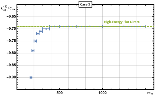
Figure 4: Value of the ratio $C_{lq}^{(1)}/C_{eu}$ for Case 1 for which the SMEFT correction to $d\sigma/dm_{ll}$ vanishes as a function of the invariant mass bins considered in Ref. [37]. This is compared to the predicted value in the $\hat{s}\gg M_{Z}^{2}$ limit. The horizontal bars indicate the width of the experimental mass bins.

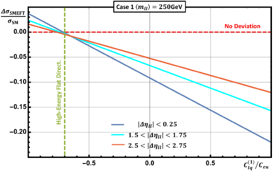
Figure 5: Deviation from the SM as a function of the ratio $C_{lq}^{(1)}/C_{eu}$ for the choice $C_{eu}=1/{\rm TeV}^{2}$ for three different $|\Delta\eta_{ll}|$ bins from Ref. [37]. The ratio for which no deviation is predicted is also shown.

We now perform separate $\chi^{2}$ fits to the LHC Drell-Yan and anticipated EIC data, fixing $C_{ed}$ as discussed above and allowing $C_{lq}^{(1)}$ and $C_{eu}$ to vary. The 68% confidence level (CL) allowed regions are shown in Fig. 6. In order to more directly compare the sensitivities of the two experiments, which is our major goal in this manuscript, we shift the best-fit values of the Wilson coefficients at the LHC to the origin.

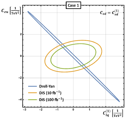
Figure 6: 68% confidence level ellipse in the $C_{lq}^{(1)}$ versus $C_{eu}$ space for Case 1. $C_{ed}$ has been set to the value indicated in the text. We contrast the confidence levels derived from the Drell-Yan data with the projected regions for a $10\,\textrm{fb}^{-1}$ and $100\,\textrm{fb}^{-1}$ EIC.

As we can see in Fig. 6 the Drell-Yan data is only able to constrain the absolute values of $C_{lq}^{(1)}$ and $C_{eu}$ to be smaller than $3.0$ and $4.0$ respectively, in units of $1/\textrm{TeV}^{2}$. The projected EIC bounds are more stringent, $1.5$ and $1.0$ respectively. Increasing the integrated luminosity from $10\,\textrm{fb}^{-1}$ to $100\,\textrm{fb}^{-1}$ moderately tightens the expected bounds. The plot illustrates that the two Wilson coefficients are highly correlated in the case of Drell-Yan observables, as evident from the tight but elongated ellipse. With DIS data the ellipses are less correlated. The approximate flat direction is broken through the interplay of different polarized observables.

Ultimately we wish to combine the results from both experiments to provide the strongest probes of the Wilson coefficients. This would approximately constrain the possible parameter space to the overlap of the two respective ellipses. This is indeed what we find in Fig. 7, where a combined fit to both the EIC and LHC data sets is compared to each experiment alone. Each Wilson coefficient is separately constrained to have a magnitude below one. The allowed parameter values along the flat direction poorly probed by the LHC are reduced by more than a factor of three in this combined fit.

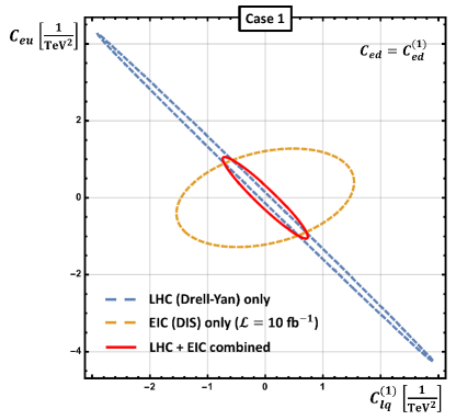
Figure 7: 68% confidence level ellipse in the $C_{lq}^{(1)}$ versus $C_{eu}$ space for Case 1 with only LHC data, only EIC data, and after combining both experiments.

6.2 Case 2

We next consider the case when $C_{eu}$, $C_{ed}$ and $C_{qe}$ are non-zero. Since the $C_{qe}$ dependence of the Drell-Yan matrix element occurs in the $\hat{t}^{2}$ term while the other Wilson coefficients contribute to the $\hat{u}^{2}$ terms these coefficients are in principle distinguishable. However, as argued above the nature of the studied experimental measurement at the LHC cannot distinguish between these coefficients. To demonstrate this we show in Fig. 8 the SMEFT-induced deviation for the $|\Delta\eta_{ll}|$ distribution as a function of the ratio $C_{qe}/C_{eu}$ for the mass bin $M_{ll}=[200,300]$ GeV. By integrating over $c_{\theta}$ we can find the predicted high-energy flat direction:

$$C_{qe} = -C_{eu}\frac{Q_{u}e^{2}-g_{Z}^{2}g_{L}^{u}g_{R}^{e}}{Q_{u}e^{2}-g_{Z}^{2}g_{R}^{e}g_{R}^{u}}\approx-0.23C_{eu},$$

$$C_{qe} = -C_{ed}\frac{Q_{d}e^{2}-g_{Z}^{2}g_{L}^{d}g_{R}^{e}}{Q_{d}e^{2}-g_{Z}^{2}g_{R}^{e}g_{R}^{d}}\approx 0.54C_{ed}.$$ (25)

As before we set $C_{ed}=C_{ed}^{(2)}$ with

$$C_{ed}^{(2)}=C_{eu}\frac{Q_{u}e^{2}-g_{Z}^{2}g_{L}^{u}g_{R}^{e}}{Q_{u}e^{2}-g_{Z}^{2}g_{R}^{e}g_{R}^{u}}\frac{Q_{d}e^{2}-g_{Z}^{2}g_{R}^{e}g_{R}^{d}}{Q_{d}e^{2}-g_{Z}^{2}g_{L}^{d}g_{R}^{e}}$$ (26)

the value required to simultaneously satisfy both equations above. We see in Fig. 8 that the SMEFT-induced deviation for all bins vanishes near the predicted value, again demonstrating that this distribution cannot discriminate Wilson coefficients near the flat direction.

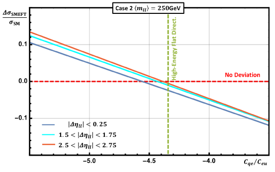
Figure 8: Deviation from the SM as a function of the ratio $C_{qe}/C_{eu}$ for the choice $C_{eu}=1/{\rm TeV}^{2}$ for three different $|\Delta\eta_{ll}|$ bins from Ref. [37]. The ratio for which no deviation is predicted is also shown.

We perform similar $\chi^{2}$ fits as done for Case 1 above. The resulting bounds can be seen in Fig. 9.

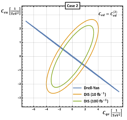
Figure 9: 68% confidence level ellipse in the $C_{qe}$ versus $C_{eu}$ space for Case 2. $C_{ed}$ has been set to the value indicated in the text. We contrast the confidence levels derived from the Drell-Yan data with the projected regions for a $10\,\textrm{fb}^{-1}$ and $100\,\textrm{fb}^{-1}$ EIC.

Similar to Case 1 the Drell-Yan data constrains the absolute values of $C_{qe}$ and $C_{eu}$ to be smaller than roughly $7$ and $2.5$ respectively in units of $1/\textrm{TeV}^{2}$. The EIC ellipses are similar in magnitude with a projected constraint for $C_{qe}$ between about $-4$ and $4$ and $-2.5$ and $2.5$ for $C_{eu}$. Once again, since there is a flat direction present in the Drell-Yan expressions the corresponding ellipse is highly correlated, which is not the case at the EIC. Combining both experiments would allow us to constrain both parameters to roughly unity. We show this in Fig. 10 with a combined fit to both the EIC and LHC data sets, compared to each experiment alone. The ellipse indicating the allowed region is still elongated along the direction poorly probed by the Drell-Yan data, but the allowed parameter values are reduced by nearly a factor of three.

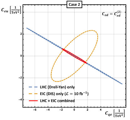
Figure 10: 68% confidence level ellipse in the $C_{qe}$ versus $C_{eu}$ space for Case 2 with only LHC data, only EIC data, and after combining both experiments.

6.3 Case 3

We now consider Case 3, where both $C_{qe}$ and $C_{lq}^{(1)}$ are non-zero. In the high-energy limit of the Drell-Yan cross section, flat directions exist separately in the up-quark and down-quark channels. Assuming a symmetric integration over $c_{\theta}$ they can be found to be:

• Up-quark:

  $$C_{lq}^{(1)}=-C_{qe}\frac{Q_{u}e^{2}-g_{Z}^{2}g_{L}^{u}g_{R}^{e}}{Q_{u}e^{2}-g_{Z}^{2}g_{L}^{e}g_{L}^{u}}\approx-0.16C_{qe}.$$ (27)

• Down-quark:

  $$C_{lq}^{(1)}=-C_{qe}\frac{Q_{d}e^{2}-g_{Z}^{2}g_{L}^{d}g_{R}^{e}}{Q_{u}e^{2}-g_{Z}^{2}g_{L}^{e}g_{L}^{d}}\approx 0.22C_{qe}.$$ (28)

These two equations for $C_{lq}^{(1)}$ and $C_{qe}$ cannot be simultaneously satisfied, indicating that Drell-Yan measurements should be able to better probe this choice of parameters than the two cases considered previously. We show the projected bounds in Fig. 11.

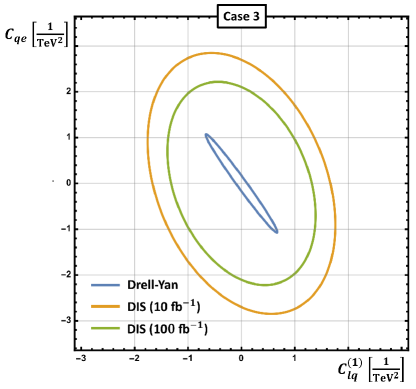
Figure 11: 68% confidence level ellipse in the $C_{qe}$ versus $C_{lq}^{(1)}$ space for Case 3. We contrast the confidence levels derived from the Drell-Yan data with the projected regions for a $10\,\textrm{fb}^{-1}$ and $100\,\textrm{fb}^{-1}$ EIC.

The EIC bounds derived for $C_{lq}^{(1)}$ and $C_{qe}$ are similar to the ones in Case 1 and 2 and constrain the absolute values of the coefficients to be smaller than about $1.5$ and $2.5$ respectively. There is very little correlation between the coefficients as evident from the ellipses. The Drell-Yan bounds are significantly tighter than the DIS bounds in Case 3. This is expected since there is no flat direction involving $C_{lq}^{(1)}$ and $C_{qe}$ in Drell-Yan. This case illustrates the power of the Drell-Yan data in the absence of flat directions; the bounds obtained are nearly an order of magnitude stronger than the Drell-Yan bounds found for Cases 1 and 2.

6.4 Case 4

Finally, we consider $C_{lq}^{(1)}$ and $C_{lq}^{(3)}$ non-zero. The Drell-Yan up-quark channel depends on the combination $C_{lq}^{(1)}-C_{lq}^{(3)}$ while the down-quark channel depends on $C_{lq}^{(1)}+C_{lq}^{(3)}$. In principle these two Wilson coefficients are distinguishable through the different kinematics of these two channels. In DIS we can directly access $C_{lq}^{(3)}$ through charged-current scattering. At the LHC this would be possible if an analysis similar to Ref. [37] were performed for off-shell $W$-boson production. We are not aware of such an analysis.

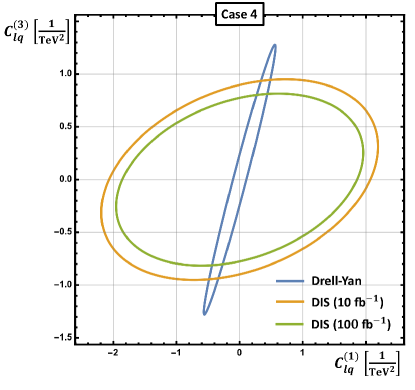
Figure 12: 68% confidence level ellipse in the $C_{lq}^{(3)}$ versus $C_{lq}^{(1)}$ space for Case 4. We contrast the confidence levels derived from the Drell-Yan data with the projected regions for a $10\,\textrm{fb}^{-1}$ and $100\,\textrm{fb}^{-1}$ EIC.

We present the bounds obtained for the LHC and EIC in Fig. 12. The bounds obtained from the Drell-Yan data are stronger than in Cases 1 and 2. This finding is consistent with the absence of a flat direction due to the different dependences on $C_{lq}^{(1)}$ and $C_{lq}^{(3)}$. The constraint on $C_{lq}^{(1)}$ reaches below $1$. The bounds can be improved through the inclusion of EIC charged-current data which are exclusively sensitive to $C_{lq}^{(3)}$.

6.5 Effects of parameter choices on EIC fits

We study here the impact of EIC systematic error and polarization on the results obtained above, using Case 3 as a representative example. Our results are shown in Fig. 13. We see that increasing the systematic error from 1% to 2% has little impact on the analysis. However, it is clear that the ability of the EIC to measure polarized observables is crucial in obtaining strong probes of Wilson coefficients. The projected bounds weaken by a factor of four if polarized observables are removed from the fit. We have additionally investigated the effect of increasing the polarization of the electron beam to $\lambda_{e}=0.85$ and $\lambda_{e}=0.95$. The impact on the bounds and the correlation of the ellipses is negligible.

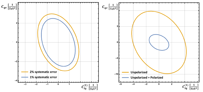
Figure 13: Example $68\%$ CL ellipses for different choices of the systematic error (left) and upon removing polarized observables (right).

7 Conclusions

We have studied in this paper the potential of future EIC measurements to probe dimension-6 operators in the SMEFT. The possibility of measuring polarized cross sections at an EIC provides a powerful handle on four-fermion operators in the SMEFT. In particular, the ability to measure both the unpolarized and polarized proton cross sections with different electron polarizations allows the effects of different Wilson coefficients to be disentangled. This discrimination between dimension-6 effects is not possible with just Drell-Yan data at the LHC, where only limited combinations of Wilson coefficients are accessible. In addition, the absence of high invariant-mass measurements of quantities such as a forward-backward asymmetry at the LHC further limits the ability of the Drell-Yan data to disentangle the various dimension-6 effects. We demonstrate these points by example fits to both available LHC data and projected EIC data in four different scenarios that illustrate the flat directions present with only Drell-Yan invariant mass data available. We show that fits including both LHC and future EIC data provide much stronger constraints on the Wilson coefficients than fits to either experiment separately.

References

- [1] W. Buchmuller and D. Wyler, Nucl. Phys. B 268, 621 (1986). doi:10.1016/0550-3213(86)90262-2
- [2] B. Grzadkowski, M. Iskrzynski, M. Misiak and J. Rosiek, JHEP 1010, 085 (2010) doi:10.1007/JHEP10(2010)085 [arXiv:1008.4884 [hep-ph]].
- [3] Z. Han and W. Skiba, Phys. Rev. D 71, 075009 (2005) doi:10.1103/PhysRevD.71.075009 [hep-ph/0412166].
- [4] A. Pomarol and F. Riva, JHEP 1401, 151 (2014) doi:10.1007/JHEP01(2014)151 [arXiv:1308.2803 [hep-ph]].
- [5] C. Y. Chen, S. Dawson and C. Zhang, Phys. Rev. D 89, no. 1, 015016 (2014) doi:10.1103/PhysRevD.89.015016 [arXiv:1311.3107 [hep-ph]].
- [6] J. Ellis, V. Sanz and T. You, JHEP 1407, 036 (2014) doi:10.1007/JHEP07(2014)036 [arXiv:1404.3667 [hep-ph]].
- [7] J. D. Wells and Z. Zhang, Phys. Rev. D 90, no. 3, 033006 (2014) doi:10.1103/PhysRevD.90.033006 [arXiv:1406.6070 [hep-ph]].
- [8] A. Falkowski and F. Riva, JHEP 1502, 039 (2015) doi:10.1007/JHEP02(2015)039 [arXiv:1411.0669 [hep-ph]].
- [9] J. de Blas, M. Ciuchini, E. Franco, S. Mishima, M. Pierini, L. Reina and L. Silvestrini, JHEP 1612, 135 (2016) doi:10.1007/JHEP12(2016)135 [arXiv:1608.01509 [hep-ph]].
- [10] V. Cirigliano, W. Dekens, J. de Vries and E. Mereghetti Phys. Rev. D 94, no. 3, 034031 (2016) doi:10.1103/PhysRevD.94.034031 [arXiv:1605.04311 [hep-ph]].
- [11] A. Biekoetter, T. Corbett and T. Plehn, SciPost Phys. 6, no. 6, 064 (2019) doi:10.21468/SciPostPhys.6.6.064 [arXiv:1812.07587 [hep-ph]].
- [12] C. Grojean, M. Montull and M. Riembau, JHEP 03, 020 (2019) doi:10.1007/JHEP03(2019)020 [arXiv:1810.05149 [hep-ph]].
- [13] N. P. Hartland, F. Maltoni, E. R. Nocera, J. Rojo, E. Slade, E. Vryonidou and C. Zhang, JHEP 1904, 100 (2019) doi:10.1007/JHEP04(2019)100 [arXiv:1901.05965 [hep-ph]].
- [14] I. Brivio, S. Bruggisser, F. Maltoni, R. Moutafis, T. Plehn, E. Vryonidou, S. Westhoff and C. Zhang, JHEP 2002, 131 (2020) doi:10.1007/JHEP02(2020)131 [arXiv:1910.03606 [hep-ph]].
- [15] G. Passarino and M. Trott, arXiv:1610.08356 [hep-ph].
- [16] B. Henning, X. Lu, T. Melia and H. Murayama, JHEP 1708, 016 (2017) Erratum: [JHEP 1909, 019 (2019)] doi:10.1007/JHEP09(2019)019, 10.1007/JHEP08(2017)016 [arXiv:1512.03433 [hep-ph]].
- [17] C. Degrande, JHEP 1402, 101 (2014) doi:10.1007/JHEP02(2014)101 [arXiv:1308.6323 [hep-ph]].
- [18] A. Azatov, R. Contino, C. S. Machado and F. Riva, Phys. Rev. D 95, no. 6, 065014 (2017) doi:10.1103/PhysRevD.95.065014 [arXiv:1607.05236 [hep-ph]].
- [19] C. Hays, A. Martin, V. Sanz and J. Setford, JHEP 1902, 123 (2019) doi:10.1007/JHEP02(2019)123 [arXiv:1808.00442 [hep-ph]].
- [20] S. Alioli, R. Boughezal, E. Mereghetti and F. Petriello, [arXiv:2003.11615 [hep-ph]].
- [21] E. Keilmann and W. Shepherd, JHEP 1909, 086 (2019) doi:10.1007/JHEP09(2019)086 [arXiv:1907.13160 [hep-ph]].
- [22] A. Azatov and A. Paul, JHEP 1401, 014 (2014) doi:10.1007/JHEP01(2014)014 [arXiv:1309.5273 [hep-ph]].
- [23] A. Falkowski, M. González-Alonso and K. Mimouni, JHEP 1708, 123 (2017) doi:10.1007/JHEP08(2017)123 [arXiv:1706.03783 [hep-ph]].
- [24] S. Dawson, P. P. Giardino and A. Ismail, Phys. Rev. D 99, no. 3, 035044 (2019) doi:10.1103/PhysRevD.99.035044 [arXiv:1811.12260 [hep-ph]].
- [25] S. Alte, M. König and W. Shepherd, JHEP 1907, 144 (2019) doi:10.1007/JHEP07(2019)144 [arXiv:1812.07575 [hep-ph]].
- [26] T. Hurth, S. Renner and W. Shepherd, JHEP 06, 029 (2019) doi:10.1007/JHEP06(2019)029 [arXiv:1903.00500 [hep-ph]].
- [27] R. Aoude, T. Hurth, S. Renner and W. Shepherd, [arXiv:2003.05432 [hep-ph]].
- [28] A. Accardi et al., Eur. Phys. J. A 52, no. 9, 268 (2016) doi:10.1140/epja/i2016-16268-9 [arXiv:1212.1701 [nucl-ex]].
- [29] E. B. Zijlstra and W. L. van Neerven, Nucl. Phys. B 383, 525 (1992). doi:10.1016/0550-3213(92)90087-R
- [30] E. B. Zijlstra and W. L. van Neerven, Nucl. Phys. B 417, 61 (1994) Erratum: [Nucl. Phys. B 426, 245 (1994)] Erratum: [Nucl. Phys. B 773, 105 (2007)] Erratum: [Nucl. Phys. B 501, 599 (1997)]. doi:10.1016/0550-3213(94)90538-X, 10.1016/0550-3213(94)90135-X, 10.1016/S0550-3213(97)00389-1, 10.1016/j.nuclphysb.2007.03.002
- [31] A. Denner, Fortsch. Phys. 41, 307 (1993) doi:10.1002/prop.2190410402 [arXiv:0709.1075 [hep-ph]].
- [32] M. Tanabashi et al. [Particle Data Group], Phys. Rev. D 98, no. 3, 030001 (2018). doi:10.1103/PhysRevD.98.030001s
- [33] R. D. Ball et al. [NNPDF Collaboration], Eur. Phys. J. C 77, no. 10, 663 (2017) doi:10.1140/epjc/s10052-017-5199-5 [arXiv:1706.00428 [hep-ph]].
- [34] E. R. Nocera et al. [NNPDF Collaboration], Nucl. Phys. B 887, 276 (2014) doi:10.1016/j.nuclphysb.2014.08.008 [arXiv:1406.5539 [hep-ph]].
- [35] E. C. Aschenauer, T. Burton, T. Martini, H. Spiesberger and M. Stratmann, Phys. Rev. D 88, 114025 (2013) doi:10.1103/PhysRevD.88.114025 [arXiv:1309.5327 [hep-ph]].
- [36] X. Chu, E. C. Aschenauer, J. H. Lee and L. Zheng, Phys. Rev. D 96, no. 7, 074035 (2017) doi:10.1103/PhysRevD.96.074035 [arXiv:1705.08831 [nucl-ex]].
- [37] G. Aad et al. [ATLAS Collaboration], JHEP 1608, 009 (2016) doi:10.1007/JHEP08(2016)009 [arXiv:1606.01736 [hep-ex]].
- [38] S. Carrazza, C. Degrande, S. Iranipour, J. Rojo and M. Ubiali, Phys. Rev. Lett. 123, no. 13, 132001 (2019) doi:10.1103/PhysRevLett.123.132001 [arXiv:1905.05215 [hep-ph]].
- [39] V. Khachatryan et al. [CMS Collaboration], Eur. Phys. J. C 76, no. 6, 325 (2016) doi:10.1140/epjc/s10052-016-4156-z [arXiv:1601.04768 [hep-ex]].
- [40] A. M. Sirunyan et al. [CMS Collaboration], Eur. Phys. J. C 78, no. 9, 701 (2018) doi:10.1140/epjc/s10052-018-6148-7 [arXiv:1806.00863 [hep-ex]].
- [41] M. Aaboud et al. [ATLAS Collaboration], JHEP 1712, 059 (2017) doi:10.1007/JHEP12(2017)059 [arXiv:1710.05167 [hep-ex]].