LQG Graphon Mean Field Games:
Analysis via Graphon Invariant Subspaces

Abstract

This paper studies approximate solutions to large-scale linear quadratic stochastic games with homogeneous nodal dynamics parameters and heterogeneous network couplings within the graphon mean field game framework in [2, 3, 4]. A graphon time-varying dynamical system model is first formulated to study the finite and then limit problems of linear quadratic Gaussian graphon mean field games (LQG-GMFG). The Nash equilibrium of the limit problem is then characterized by two coupled graphon time-varying dynamical systems. Sufficient conditions are established for the existence of a unique solution to the limit LQG-GMFG problem. For the computation of LQG-GMFG solutions two methods are established and employed where one is based on fixed point iterations and the other on a decoupling operator Riccati equation; furthermore, two corresponding sets of solutions are established based on spectral decompositions. Finally, a set of numerical simulations on networks associated with different types of graphons are presented.

I Introduction

Many applications such as market networks, large-scale social networks, advertising networks, communication networks and smart grids involve strategic decisions over a large number of agents coupled via large-scale heterogeneous network structures. The large cardinalities of the underlying networks and the complexity of the underlying network couplings in dynamics and decision strategies make such problems challenging or even intractable by standard methods. To characterize large graphs and study the convergence of dense graph sequences to their limits, graphon theory is established in the combinatorics and computer science communities [5, 6, 7]. It has been applied to study dynamical systems [8, 9, 10, 11], network centrality [12], random walks [13], signal processing [14], graph neural networks [15], epidemic models [16, 17], Graphon Control of very large-scale networks [18, 19, 20, 16, 21, 22], and static and dynamic game problems on graphons [23, 24, 2, 3, 4, 25, 26]. In order to study strategic decision problems for finite populations on finite networks, game theoretic models with various interpretations of the underlying networks have been developed by various authors (see for instance [27, 28, 29, 30]). Passing to large population problems on large networks, Graphon Mean Field Game (GMFG) theory was proposed and developed in [2, 3, 4], which generalizes the classical mean field game theory in the sense that each node may be influenced by a different local mean field. Under suitable technical conditions, Nash equilibria and $\varepsilon$-Nash properties have been established in [2, 3, 4]. Mean field game problems with non-uniform cost couplings were studied in an earlier paper [31], and mean field game problems on graphs with different interpretations of the underlying graphs have also been treated in [32, 33, 34]. In [32, 33], the graph represents physical constraints on the state space of the mean field game problems. In [34] linear quadratic mean field games over Erdös-Rényi graphs are studied where the associated asymptotic game is a classical mean field game. Recent works on mean field game problems on networks include [35, 26].

There are two classes of closely related mean field game problems on networks in the papers above depending on the definitions of nodes: (i) networks of mean field (or measure) couplings where each node on the network represents a population [2, 3, 4]; (ii) networks of individual state couplings where each node represents an agent (see for instance [25, 31, 34, 35, 26]). In the current paper, each node represents a population of homogenous agents.

The LQG-GMFG strategy in this current paper is as follows: first we identify the limit system when the size of the local nodal population and the size of the graph go to infinity; the Nash equilibrium for the limit system is then characterized by two coupled (global) graphon dynamical system equations; finally, each agent can then identify an approximated Nash strategy for the original LQG dynamic games on networks following the Nash equilibrium for the limit system.

The main contributions of this paper include:

• the characterization of the solution to the limit LQG-GMFG problem by two coupled (global) graphon time-varying dynamical systems;

• sufficient conditions on the existence of a unique solution to the limit LQG-GMFG problem;

• two spectral-based solution methods for solving the limit LQG-GMFG problems, one based on fixed point iterations and the other based on a decoupling operator Riccati equation.

Notation: $\mathds{R}$ denotes the set of real numbers. Bold face letters (e.g. $\mathbf{A}$, $\mathbf{B}$, $\mathbf{u}$) are used to represent graphons, compact operators and functions. Blackboard bold letters (e.g. $\mathbb{A}$, $\mathbb{B}$) are used to denote linear operators which are not necessarily compact. $\mathbb{A}^{\mathchoice{\raisebox{0.0pt}{$\displaystyle\intercal$}}{\raisebox{0.0pt}{$\textstyle\intercal$}}{\raisebox{0.0pt}{$\scriptstyle\intercal$}}{\raisebox{0.0pt}{$\scriptscriptstyle\intercal$}}}$ denotes the adjoint operator of $\mathbb{A}$. $\mathcal{W}_{c}$ denotes the set of all symmetric bounded measurable functions $\mathbf{W}:[0,1]^{2}\rightarrow[-c,c]$ with $c>0$; $\mathcal{W}_{0}$ denotes the set of all symmetric measurable functions $\mathbf{W}:[0,1]^{2}\rightarrow[0,1]$. For a Hilbert space $\mathcal{H}$, let $\mathcal{L}(\mathcal{H})$ denote the Banach algebra of bounded linear operators from $\mathcal{H}$ to $\mathcal{H}$. $\mathcal{L}(\mathcal{H})$ endowed with the uniform operator topology is denoted by $\mathcal{L}_{u}(\mathcal{H})$. $C([0,T];\mathcal{X})$ denotes the set of continuous functions from $[0,T]$ to a Banach space $\mathcal{X}$. Let $\oplus$ denote direct sum. Let $\otimes$ denote matrix Kronecker product. For any matrix $Q\in\mathds{R}^{n\times n}$, $Q\geq 0$ (resp. $Q>0$) means $Q^{\mathchoice{\raisebox{0.0pt}{$\displaystyle\intercal$}}{\raisebox{0.0pt}{$\textstyle\intercal$}}{\raisebox{0.0pt}{$\scriptstyle\intercal$}}{\raisebox{0.0pt}{$\scriptscriptstyle\intercal$}}}=Q$ and $x^{\mathchoice{\raisebox{0.0pt}{$\displaystyle\intercal$}}{\raisebox{0.0pt}{$\textstyle\intercal$}}{\raisebox{0.0pt}{$\scriptstyle\intercal$}}{\raisebox{0.0pt}{$\scriptscriptstyle\intercal$}}}Qx\geq 0$ (resp. $x^{\mathchoice{\raisebox{0.0pt}{$\displaystyle\intercal$}}{\raisebox{0.0pt}{$\textstyle\intercal$}}{\raisebox{0.0pt}{$\scriptstyle\intercal$}}{\raisebox{0.0pt}{$\scriptscriptstyle\intercal$}}}Qx>0$) for all $x\in\mathds{R}^{n}$. For $x\in\mathds{R}^{n}$, $Q\in\mathds{R}^{n\times n}$ and $Q\geq 0$, let $\|x\|_{Q}^{2}\triangleq x^{\mathchoice{\raisebox{0.0pt}{$\displaystyle\intercal$}}{\raisebox{0.0pt}{$\textstyle\intercal$}}{\raisebox{0.0pt}{$\scriptstyle\intercal$}}{\raisebox{0.0pt}{$\scriptscriptstyle\intercal$}}}Qx$. Let $(L^{2}[0,1])^{n}\triangleq\underbrace{L^{2}[0,1]\times\cdots\times L^{2}[0,1]}_{n}.$ The inner product in $(L^{2}[0,1])^{n}$ is defined as follows: for $\mathbf{v},\mathbf{u}\in(L^{2}[0,1])^{n}$, $\langle\mathbf{u},\mathbf{v}\rangle\triangleq\sum_{i=1}^{n}\int_{[0,1]}\mathbf{v}_{i}(\alpha)\mathbf{u}_{i}(\alpha)d\alpha=\int_{[0,1]}\langle\mathbf{v}(\alpha),\mathbf{u}(\alpha)\rangle_{\mathds{R}^{n}}d\alpha$ where $\mathbf{u}_{i}(\cdot)\in L^{2}[0,1]$ with $i\in\{1,\ldots,n\}$ denotes the $i$th component of $\mathbf{u}$ and $\mathbf{u}(\alpha)\in\mathds{R}^{n}$ denotes the vector associated with index $\alpha\in[0,1]$. The space $(L^{2}[0,1])^{n}$ with the above inner product is a Hilbert space with the corresponding norm $\|\mathbf{v}\|_{(L^{2}[0,1])^{n}}\triangleq\left(\int_{[0,1]}\|\mathbf{v}(\alpha)\|_{\mathds{R}^{n}}^{2}d\alpha\right)^{\frac{1}{2}}.$ We use $L^{2}([0,T];(L^{2}[0,1])^{n})$ to denote the Hilbert space of equivalence classes of strongly measurable (in the Böchner sense [36, p.103]) mappings from $[0,T]$ to $(L^{2}[0,1])^{n}$ that are integrable with the norm $\|\mathbf{x}\|_{L^{2}([0,T];(L^{2}[0,1])^{n})}=\Big{(}\int_{0}^{T}\|\mathbf{x}(t)\|^{2}_{(L^{2}[0,1])^{n}}dt\Big{)}^{\frac{1}{2}}.$ The function $\mathbf{1}\in L^{2}[0,1]$ is defined as follows: for all $\alpha\in[0,1]$, $\mathbf{1}(\alpha)=1$. For any vector $v\in\mathds{R}^{n}$, $v\mathbf{1}$ denotes the function in $(L^{2}[0,1])^{n}$ such that $(v\mathbf{1})(\alpha)=v$ for all $\alpha\in[0,1]$. $\mathbf{1}_{n}$ denotes the $n$-dimensional vector of ones and $I_{{}_{N}}$ denotes the identity matrix of dimension $N\times N$. For any two functions $f$ and $g$ defined on subsets of $\mathds{R}$, $f=O(g)$ means that there exist a positive real constant $c$ and a number $x_{0}$ such that $|f(x)|\leq cg(x)$ holds for all $x\geq x_{0}$.

II Preliminaries

II-A Graphs, Graphons and Graphon Operators

A graph $G=(V,E)$ is specified by a node set $V=\{1,...,N\}$ and an edge set $E\subset V\times V$. The corresponding adjacency matrix $W=[w_{ij}]$ is defined as follows: $w_{ij}=1$ if $(i,j)\in E$; otherwise $w_{ij}=0$. A graph is undirected if its edge pair is unordered. For a weighted undirected graph, $w_{ij}$ in its adjacency matrix $W$ is given by the weight between nodes $i$ and $j$. Furthermore an adjacency matrix can be represented as a pixel diagram on the unit square $[0,1]^{2}\subset\mathds{R}^{2}$, which corresponds to a graphon step function [7] (see Fig. 1).

Graphons are defined as bounded symmetric Lebesgue measurable functions $\mathbf{M}:[0,1]^{2}\rightarrow[0,1]$. The space of graphons endowed with the cut metric (see [7]) allows the definition of the convergence of graph sequences. In this paper, we consider bounded symmetric Lebesgue measurable functions $\mathbf{M}:[0,1]^{2}\rightarrow[-c,c]$ with $c>0$, and the space of all such functions is denoted by $\mathcal{W}_{c}$. The space $\mathcal{W}_{c}$ is compact under the cut metric after identifying equivalent points of cut distance zero [7].

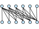
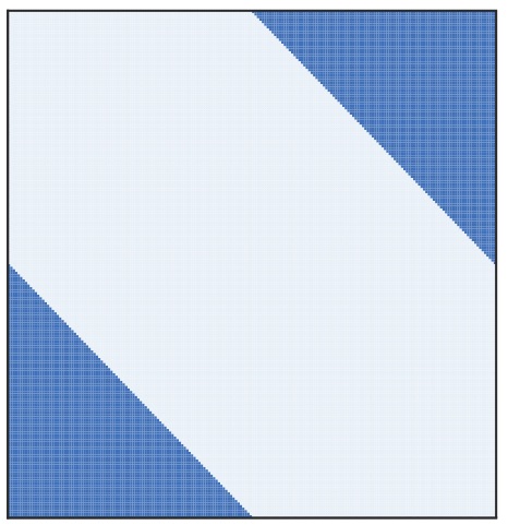
Figure 1: A half graph [7], its pixel diagram, and its limit graphon

A graphon $\mathbf{M}\in\mathcal{W}_{c}$ also defines a self-adjoint bounded linear operator from $L^{2}[0,1]$ to $L^{2}[0,1]$ as follows:

$$(\mathbf{M}\mathbf{u})(\alpha)=\int_{[0,1]}\mathbf{M}(\alpha,\eta)\mathbf{u}(\eta)d\eta,\quad\forall\alpha\in[0,1],$$ (1)

where $\mathbf{u},~{}\mathbf{M}\mathbf{u}\in L^{2}[0,1]$. Moreover, graphons can be associated with operators from $(L^{2}[0,1])^{n}$ to $(L^{2}[0,1])^{n}$. Let $\mathcal{L}\left(\left(L^{2}[0,1]\right)^{n}\right)$ represent the set of bounded linear operators from $\left(L^{2}[0,1]\right)^{n}$ to $\left(L^{2}[0,1]\right)^{n}$. For any general bounded linear operator $\mathbb{T}\in\mathcal{L}\left(L^{2}[0,1]\right)$ and $D\in\mathds{R}^{n\times n}$, the operator $[D\mathbb{T}]\in\mathcal{L}\left((L^{2}[0,1])^{n}\right)$ is defined as follows: for any $\mathbf{v}\in\left(L^{2}[0,1]\right)^{n}$ and any index $\alpha\in[0,1]$,

$$([D\mathbb{T}]\mathbf{v})(\alpha)\triangleq D\begin{pmatrix}(\mathbb{T}\mathbf{v}_{1})(\alpha)\\ \vdots\\ (\mathbb{T}\mathbf{v}_{n})(\alpha)\end{pmatrix}\in\mathds{R}^{n},$$ (2)

where $\mathbf{v}_{i}\in L^{2}[0,1]$ denotes the $i$th component of $\mathbf{v}\in(L^{2}[0,1])^{n}$. We use the square bracket $[\cdot]$ in (2) to indicate that the operator is in $\mathcal{L}\left(\left(L^{2}[0,1]\right)^{n}\right)$. The $k$th $(k\geq 0)$ power functions of $[D\mathbb{T}]$ and is given by $[D\mathbb{T}]^{k}=[D^{k}\mathbb{T}^{k}]$ where $\mathbb{T}^{0}$ is formally defined as the identity operator from $L^{2}[0,1]$ to $L^{2}[0,1]$. Following (2), the operator $[D\mathbf{M}]\in\mathcal{L}\left(\left(L^{2}[0,1]\right)^{n}\right)$ with $D\in\mathds{R}^{n\times n}$ and $\mathbf{M}\in\mathcal{W}_{c}$ is therefore defined as follows: for any $\mathbf{v}\in\left(L^{2}[0,1]\right)^{n}$ and any index $\alpha\in[0,1]$,

$$([D\mathbf{M}]\mathbf{v})(\alpha) \triangleq D\begin{pmatrix}(\mathbf{M}\mathbf{v}_{1})(\alpha)\\ \vdots\\ (\mathbf{M}\mathbf{v}_{n})(\alpha)\end{pmatrix}\in\mathds{R}^{n}.$$ (3)

Since $[D\mathbf{M}]$ is a bounded linear operator from $\left(L^{2}([0,1])\right)^{n}$ to $\left(L^{2}([0,1])\right)^{n}$, it generates a uniformly continuous (hence strongly continuous) semigroup [37] given by $S_{[D\mathbf{M}]}(t)=\textup{exp}{\left(t[D\mathbf{M}]\right)}\triangleq\sum_{k=0}^{\infty}\frac{1}{k!}t^{k}[D\mathbf{M}]^{k},~{}t\geq 0.$ Following the definition in (2), for the identity operator $\mathbb{I}\in\mathcal{L}\left(L^{2}[0,1]\right)$ and $D\in\mathds{R}^{n\times n}$, the operation $[D\mathbb{I}]$ satisfies the following: for any $\mathbf{v}\in\left(L^{2}[0,1]\right)^{n}$ and any index $\alpha\in[0,1]$,

$$([D\mathbb{I}]\mathbf{v})(\alpha)\triangleq D\begin{pmatrix}\mathbf{v}_{1}(\alpha)~{}\ldots~{}\mathbf{v}_{n}(\alpha)\end{pmatrix}^{\mathchoice{\raisebox{0.0pt}{$\displaystyle\intercal$}}{\raisebox{0.0pt}{$\textstyle\intercal$}}{\raisebox{0.0pt}{$\scriptstyle\intercal$}}{\raisebox{0.0pt}{$\scriptscriptstyle\intercal$}}}=D\mathbf{v}(\alpha)\in\mathds{R}^{n}.$$

II-B Invariant Subspace and Component-Wise Decomposition

Let $\mathcal{H}$ denote a Hilbert space. An invariant subspace of a bounded linear operator $\mathbb{T}\in\mathcal{L}(\mathcal{H})$ is defined as any subspace $\mathcal{S}_{\mathcal{H}}\subset\mathcal{H}$ such that $\mathbb{T}\mathcal{S}_{\mathcal{H}}\subset\mathcal{S}_{\mathcal{H}}.$ Then the subspace $\mathcal{S}_{\mathcal{H}}$ is called $\mathbb{T}$-invariant. Since a graphon $\mathbf{M}\in\mathcal{W}_{c}$ defines a self-adjoint operator as in (1), for any invariant subspace $\mathcal{S}\subset L^{2}[0,1]$ of $\mathbf{M}$, $\mathcal{S}^{\perp}$ is also an invariant subspace of $\mathbf{M}$ (see [22]) where $S^{\perp}$ denotes the orthogonal complement subspace of $\mathcal{S}$ in $L^{2}[0,1]$. The kernel (or nullspace) of $\mathbf{M}\in\mathcal{W}_{c}$ is denoted as $\ker(\mathbf{M})\triangleq\left\{\mathbf{v}\in L^{2}[0,1]:\mathbf{M}\mathbf{v}=\mathbf{0}\right\}$. By its definition, $\ker(\mathbf{M})$ is an invariant subspace of $\mathbf{M}\in\mathcal{W}_{c}$.

The characterizing graphon invariant subspace of $\mathbf{M}\in\mathcal{W}_{c}$ is the subspace $\mathcal{S}\subset L^{2}[0,1]$ such that $\mathcal{S}^{\perp}=\ker(\mathbf{M})$.

Let $(\mathcal{S})^{n}\triangleq\underbrace{\mathcal{S}\times\ldots\times\mathcal{S}}_{n}\subset(L^{2}[0,1])^{n}.$ Clearly, by definition, $(\mathcal{S}\oplus\mathcal{S}^{\perp})^{n}=(L^{2}[0,1])^{n}$. Any $\mathbf{v}\in(L^{2}[0,1])^{n}$ can be uniquely decomposed through its components as

$$\mathbf{v}_{i}=\bar{\mathbf{v}}_{i}+\mathbf{v}_{i}^{\perp},\quad\forall i\in\{1,...,n\}$$ (4)

where $\bar{\mathbf{v}}_{i}\in\mathcal{S}\subset L^{2}[0,1]$ and $\mathbf{v}_{i}^{\perp}\in\mathcal{S}^{\perp}\subset L^{2}[0,1]$. We call the decomposition in (4) the component-wise decomposition of $\mathbf{v}$ into $(\mathcal{S})^{n}$ and $(\mathcal{S}^{\perp})^{n}$, and denote it by $\mathbf{v}=\bar{\mathbf{v}}+\mathbf{v}^{\perp}$ where $\bar{\mathbf{v}}\in(\mathcal{S})^{n}$ and $\mathbf{v}^{\perp}\in(\mathcal{S}^{\perp})^{n}$ (see [22] for more details).

III Graphon Dynamical Systems

III-A Graphon Dynamical System Model

Consider the graphon time-varying dynamical system

$$\dot{\mathbf{x}}(t)=[A(t)\mathbb{I}+D(t)\mathbf{M}]\mathbf{x}(t)+[B(t)\mathbb{I}+E(t)\mathbf{M}]\mathbf{u}(t)$$ (5)

where $\mathbf{M}\in\mathcal{W}_{c}$, $\mathbf{x}(t)\in\left(L^{2}[0,1]\right)^{n}$ for each $t\in[0,T]$. The admissible control $\mathbf{u}{(\cdot)}$ lies in $L^{2}([0,T];(L^{2}[0,1])^{n})$. For any $t\in[0,T]$, $A(t)$, $B(t)$, $D(t)$ and $E(t)$ are $n\times n$ matrices; furthermore, $A(\cdot)$, $B(\cdot)$, $D(\cdot)$ and $E(\cdot)$ are assumed to be continuous from $[0,T]$ to $\mathds{R}^{n\times n}$. Let $\mathbb{A}(t)=[A(t)\mathbb{I}+D(t)\mathbf{M}]$ and $\mathbb{B}(t)=[B(t)\mathbb{I}+E(t)\mathbf{M}]$. A mild solution of (5) is defined as the solution $\mathbf{x}$ that is continuous over $[0,T]$ and satisfies the integral equation

$$\mathbf{x}(t)=\mathbf{x}_{0}+\int_{0}^{t}\left(\mathbb{A}(\tau)\mathbf{x}(\tau)+\mathbb{B}(\tau)\mathbf{u}(\tau)\right)d\tau.$$ (6)

Consider the initial value problem

$$\dot{\mathbf{x}}(t)=\mathbb{A}(t)\mathbf{x}(t),\quad\mathbf{x}(s)=\mathbf{x}_{s},\quad 0\leq s\leq t\leq T,$$ (7)

where $\mathbb{A}(t)=[A(t)\mathbb{I}+D(t)\mathbf{M}]$. Clearly $\mathbb{A}(t)$ for every $t\in[0,T]$ is bounded and continuous under the uniform operator topology. Hence the classical solution to (7) exists and is unique ([37, Thm. 5.2, Ch. 5]).

Definition 1 (Evolution Operator)

The evolution operator associated with $\mathbb{A}(\cdot)$ is defined as the two-parameter family of operators $\Phi(\cdot,\cdot)$ that satisfies $\Phi(t,s)\mathbf{x}_{s}=\mathbf{x}(t),~{}\text{for}~{}0\leq s\leq t\leq T$ where $\mathbf{x}$ denotes the classical solution to (7). _□

We note that $\mathbb{A}(t)=[A(t)\mathbb{I}+D(t)\mathbf{M}]$ is a bounded linear operator from $(L^{2}[0,1])^{n}$ to $(L^{2}[0,1])^{n}$ and $\mathbb{A}(\cdot)$ is continuous under the uniform operator topology. Hence following [37, Thm. 5.2, Ch. 5], the evolution operator $\Phi(\cdot,\cdot)$ satisfies

$$\frac{\partial\Phi(t,\tau)}{\partial t}=\mathbb{A}(t)\Phi(t,\tau),~{}\Phi(\tau,\tau)=\mathbb{I},~{}t,\tau\in[0,T],$$ (8)

in $\mathcal{L}_{u}\big{(}(L^{2}[0,1])^{n}\big{)}$ (the space of all bounded linear operators on $(L^{2}[0,1])^{n}$ under the uniform operator topology).

Lemma 1 (Mild Solution)

The system (5) has a unique mild solution $\mathbf{x}$ in $C([0,T];(L^{2}[0,1])^{n})$ given by

$$\mathbf{x}(t)=\Phi(t,0)\mathbf{x}(0)+\int_{0}^{t}\Phi(t,\tau)[B(\tau)\mathbb{I}+D(\tau)\mathbf{M}]\mathbf{u}(\tau)d\tau$$ (9)

with $\Phi(\cdot,\cdot)$ as the evolution operator associated with $[A(\cdot)\mathbb{I}+D(\cdot)\mathbf{M}]$.

Proof

Since $A(\cdot)$, $B(\cdot)$ and $D(\cdot)$ are continuous functions from $[0,T]$ to $\mathds{R}^{n\times n}$, we obtain that for any $\mathbf{v}\in(L^{2}[0,1])^{n}$, $\big{[}A(\cdot)\mathbb{I}+D(\cdot)\mathbf{M}\big{]}\mathbf{v}$ and $\big{[}B(\cdot)\mathbb{I}+D(\cdot)\mathbf{M}\big{]}\mathbf{v}$ are continuous functions from $[0,T]$ to $(L^{2}[0,1])^{n}$. By the Uniform Boundedness Principle, there exists $c>0$ such that $\left\|\big{[}B(t)\mathbb{I}+D(t)\mathbf{M}\big{]}\right\|_{\textup{op}}\leq c,~{}t\in[0,T].$ This together with $\mathbf{u}{(\cdot)}\in L^{2}([0,T];(L^{2}[0,1])^{n})$ implies

$$\Big{(}\big{[}B(t)\mathbb{I}+D(t)\mathbf{M}\big{]}\mathbf{u}{(t)}\Big{)}_{t\in[0,T]}\in L^{2}([0,T];(L^{2}[0,1])^{n}),$$

that is, it is Böchner measurable. Furthermore, we note that $(L^{2}[0,1])^{n}$ is a reflexive Banach space. Therefore, all the conditions in [38, Lem. 3.2, Prop. 3.4, Prop. 3.6, Part II] are verified and we obtain that the system (5) is well defined and has a unique mild solution and the solution is given by (9).

Lemma 2 (Classical Solution)

If $\mathbf{u}\in C([0,T];(L^{2}[0,1])^{n})$, then the system (5) has a unique classical solution $\mathbf{x}$, and the classical solution is also given by (9).

Proof

The proof follows a similar argument to that of [37, Thm.5.1, Chp.5]. First by Picard’s iterations, one can establish the existence of a unique mild solution satisfying the integral equation (6) based on the observations that $\mathbb{A}(\cdot)$ is continuous in the uniform operator topology. Then the fact that $\mathbf{x}$ lies in $C([0,T];(L^{2}[0,1])^{n})$ together with the assumption $\mathbf{u}\in C([0,T];(L^{2}[0,1])^{n})$ implies that the right-hand side of the integral equation (6) is differentiable. By differentiating both sides of (6) in the classical sense, we obtain the classical solution to (5). Clearly, from the analysis above, the unique classical solution is also given by (9) (see also [37, p. 130]).

Remark 1

Compared to [22], the graphon dynamical system model in (5) is time-varying; more specifically, the parameter matrices $A(\cdot),B(\cdot),D(\cdot)$ and $E(\cdot)$ are time-varying, but the underlying graphon $\mathbf{M}$ is time-invariant. This time-varying formulation will be used in characterizing the solutions to the limit LQG-GMFG problems via two coupled graphon time-varying differential equations (see Section IV-C).

III-B Relations with Finite Network Systems

Consider an $N$-node network with the following nodal dynamics: for $i\in\{1,...,N\}$,

$$\dot{x}_{i}(t)=A(t)x_{i}(t)+B(t)u_{i}(t)+D(t)x_{i}^{\mathcal{G}}(t)+E(t)u_{i}^{\mathcal{G}}(t)$$ (10)

where $x_{i}(t)\in\mathds{R}^{n}$ and $u_{i}(t)\in\mathds{R}^{n}$ represent respectively the state and the control of $i$th node at time $t$, and

$$x^{\mathcal{G}}_{i}(t)\triangleq\frac{1}{N}\sum_{j=1}^{N}m_{ij}x_{j}(t)\quad\text{and}\quad u_{i}^{\mathcal{G}}(t)\triangleq\frac{1}{N}\sum_{j=1}^{N}m_{ij}u_{j}(t)$$

represent respectively the network influence of states and that of the control at time $t\in[0,T]$. The coupling weights satisfy that $m_{ij}\leq c$ for all $i,j\in\{1,...,N\}$ where $c$ is the same constant for the graphon set $\mathcal{W}_{c}$. We note that problems with $m$-dimensional control inputs $(m<n)$ for the nodal dynamics can be represented by placing zeros in columns (with indices between $m$ and $n$) of $D(t)$ and $E(t)$ for all $t\in[0,T]$.

Consider a uniform partition $\{P_{1},\ldots,P_{N}\}$ of $[0,1]$ with $P_{1}=[0,\frac{1}{N}]$ and $P_{k}=(\frac{k-1}{N},\frac{k}{N}]$ for $2\leq k\leq N$. The step function graphon $\mathbf{M^{[N]}}$ that corresponds to $M_{N}\triangleq[m_{ij}]$ is defined by

$$\mathbf{M^{[N]}}(\vartheta,\varphi)\triangleq\sum_{i=1}^{N}\sum_{j=1}^{N}\mathds{1}_{{}_{P_{i}}}(\vartheta)\mathds{1}_{{}_{P_{j}}}(\varphi)m_{ij},\quad(\vartheta,\varphi)\in[0,1]^{2},$$

where $\mathds{1}_{{}_{P_{i}}}(\cdot)$ is the indicator function (that is, $\mathds{1}_{{}_{P_{i}}}(\vartheta)=1$ if $\vartheta\in P_{i}$ and $\mathds{1}_{{}_{P_{i}}}(\vartheta)=0$ if $\vartheta\notin P_{i}$). Let $\mathbf{x^{[N]}}(t)\in(L^{2}{[0,1]})^{n}$ be the piece-wise constant function (in the $\vartheta$ argument) corresponding to $x(t)\triangleq({x_{1}(t)}^{\mathchoice{\raisebox{0.0pt}{$\displaystyle\intercal$}}{\raisebox{0.0pt}{$\textstyle\intercal$}}{\raisebox{0.0pt}{$\scriptstyle\intercal$}}{\raisebox{0.0pt}{$\scriptscriptstyle\intercal$}}},...,{x_{N}(t)}^{\mathchoice{\raisebox{0.0pt}{$\displaystyle\intercal$}}{\raisebox{0.0pt}{$\textstyle\intercal$}}{\raisebox{0.0pt}{$\scriptstyle\intercal$}}{\raisebox{0.0pt}{$\scriptscriptstyle\intercal$}}})^{\mathchoice{\raisebox{0.0pt}{$\displaystyle\intercal$}}{\raisebox{0.0pt}{$\textstyle\intercal$}}{\raisebox{0.0pt}{$\scriptstyle\intercal$}}{\raisebox{0.0pt}{$\scriptscriptstyle\intercal$}}}\in\mathds{R}^{nN}$ given by $\mathbf{x}^{\mathbf{{[N]}}}_{\vartheta}(t)\triangleq\sum_{i=1}^{N}{\mathds{1}}_{{}_{P_{i}}}(\vartheta)x_{i}(t),~{}\forall\vartheta\in[0,1].$ Similarly, define $\mathbf{u^{[N]}}(t)\in(L^{2}{[0,1])^{n}}$ that corresponds to $u(t)\triangleq({u_{1}(t)}^{\mathchoice{\raisebox{0.0pt}{$\displaystyle\intercal$}}{\raisebox{0.0pt}{$\textstyle\intercal$}}{\raisebox{0.0pt}{$\scriptstyle\intercal$}}{\raisebox{0.0pt}{$\scriptscriptstyle\intercal$}}},...,{u_{N}(t)}^{\mathchoice{\raisebox{0.0pt}{$\displaystyle\intercal$}}{\raisebox{0.0pt}{$\textstyle\intercal$}}{\raisebox{0.0pt}{$\scriptstyle\intercal$}}{\raisebox{0.0pt}{$\scriptscriptstyle\intercal$}}})^{\mathchoice{\raisebox{0.0pt}{$\displaystyle\intercal$}}{\raisebox{0.0pt}{$\textstyle\intercal$}}{\raisebox{0.0pt}{$\scriptstyle\intercal$}}{\raisebox{0.0pt}{$\scriptscriptstyle\intercal$}}}\in\mathds{R}^{nN}$.

Then the network system in (10) may be compactly represented by the following graphon dynamical system

$$\dot{{\mathbf{x}}}^{\mathbf{[N]}}(t)=\left[A(t)\mathbb{I}+D(t)\mathbf{M^{[N]}}\right]\mathbf{x^{[N]}}(t)$$ (11)

$$\qquad\qquad+\left[B(t)\mathbb{I}+D(t)\mathbf{M^{[N]}}\right]\mathbf{u^{[N]}}(t),~{}~{}t\in[0,T],$$

where $\mathbf{x^{[N]}}(t),\mathbf{u^{[N]}}(t)\in(L^{2}_{pwc}{{}_{[0,1]}})^{n}$, $\mathbf{M^{[N]}}\in\mathcal{W}_{c}$ represents step function graphon couplings associated with the underlying graph (via its adjacency matrix $[m_{ij}]$), and $L^{2}_{pwc}{{[0,1]}}$ denotes the set of all piece-wise constant (over each element of the uniform partition) functions in $L^{2}{[0,1]}$.

The trajectories of the graphon dynamical system in (LABEL:equ:step-function-dynamical-system) correspond one-to-one to the trajectories of the network system in (10), following a similar proof argument to [19, Lem. 3]. Moreover, the system in (5) can represent the limit system for a sequence of systems represented in the form of (LABEL:equ:step-function-dynamical-system) when the underlying step function graphon sequence converges to a limit graphon (under suitable norms) and initial conditions converges to a limit initial condition in $(L^{2}[0,1])^{n}$, following a similar proof argument to [19, Thm. 7].

IV LQG Graphon Mean Field Games

The application of the graphon mean field games methodology to finite network game problems is as follows: by passing to the nodal population limit and then network limit, one can identify the limit equilibrium; this limit equilibrium is then used by all the agents to generate the approximation of the best response strategies. This methodology bypasses the combinatorial intractability of computing the exact Nash equilibria for dynamic game problems on large networks.

IV-A Stochastic Dynamic Games on Finite Networks

Consider an $N$-node graph where each node is associated with a homogeneous population of individual agents. Each individual agent is influenced by the mean field of its nodal population and the mean fields of other nodal populations over the graph. Let ${\cal V}_{c}$ denote the set of nodes representing the clusters and $N=|\mathcal{V}_{c}|$ denote the total number of such nodes. Let $\mathcal{C}_{q}$ denote the set of agents in the $q$th cluster. Then the total number of agents is given by $K=\sum_{q=1}^{N}|\mathcal{C}_{q}|$.

Following the problem formulation in [2, 3, 4], the dynamics of an individual agent $i\in\{1,...,K\}$ are given by

$$dx_{i}(t)=(Ax_{i}(t)+Bu_{i}(t)+Dz_{i}(t))dt+\Sigma dw_{i}(t),$$ (12)

where $t\in[0,T]$, $x_{i}(t)$, $u_{i}(t)$, and $z_{i}(t)$ are respectively the state, the control and the network empirical average in $\mathds{R}^{n}$. $\{w_{i},1\leq i\leq K\}$ are independent standard $n$-dimensional Wiener processes and are independent of the initial conditions $\{x_{i}(0),1\leq i\leq K\}$ which are also assumed to be independent. $\Sigma$ is a constant $n\times n$ matrix. We drop the time index for $A(\cdot),B(\cdot),D(\cdot)$ purely for notation simplicity. Problems with $m$-dimensional control inputs $(m<n)$ for the nodal dynamics can be represented by placing zeros in columns (with indices between $m$ and $n$) of $B$. For an agent $i\in\mathcal{C}_{q}$, the network empirical average $z_{i}(t)$ is given by

$$z_{i}(t)=\frac{1}{N}\sum_{\ell=1}^{N}m_{q\ell}\frac{1}{|\cal C_{\ell}|}\sum_{j\in\cal C_{\ell}}x_{j}(t)=\frac{1}{N}\sum_{\ell=1}^{N}m_{q\ell}\bar{x}_{\ell}(t)$$ (13)

where $M=[m_{q\ell}]$ is the adjacency matrix of the underlying graph, $\bar{x}_{\ell}(t)\triangleq\int_{\mathds{R}^{n}}x\hat{\mu}_{\ell}(t,x)dx$, and $\hat{\mu}_{\ell}(t,\cdot)$ denotes the empirical distribution of agent states in cluster $\mathcal{C}_{\ell}$ at time $t$.

The individual agent’s cost is given by

$$J_{i}(u_{i})\triangleq\mathbb{E}\Big{(}\int_{0}^{T}\big{(}\|x_{i}(t)-\nu_{i}(t)\|_{Q}^{2}+\|u_{i}(t)\|_{R}^{2}\big{)}dt\\ +\|x_{i}(T)-\nu_{i}(T)\|_{Q_{{}_{T}}}^{2}\Big{)}$$ (14)

where $Q,Q_{T}\geq 0,R>0$, $\nu_{i}(t)\triangleq H(z_{i}(t)+\eta)$, $\eta\in\mathds{R}^{n}$ and $H\in\mathds{R}^{n\times n}$. In other words, agent $i$ is trying to ensure that its state $x_{i}(t)$ tracks $\nu_{i}(t)$ for all $t\in[0,T]$ with relatively small control efforts.

Let $\gamma_{i}(\cdot,\cdot):[0,T]\times\mathcal{I}_{i}\to\mathds{R}^{n}$ denote the strategy of agent $i$, $i\in\{1,...,K\}$ where $\mathcal{I}_{i}$ denotes the information set available to agent $i$. The control of agent $i$ at time $t$ is then given by $u_{i}(t)=\gamma_{i}(t,\eta)$ with $\eta\in\mathcal{I}_{i}$. A strategy $K$-tuple $(\gamma_{1},...,\gamma_{K})$ is a Nash equilibrium if it satisfies

$$J_{i}(\gamma_{i},\gamma_{-i})\leq J_{i}(\gamma,\gamma_{-i}),\quad\forall\gamma(\cdot,\cdot):[0,T]\times\mathcal{I}_{i}\to\mathds{R}^{n},$$ (15)

for all $i\in\{1,...,K\},$ where $\gamma_{-i}\triangleq(\gamma_{1},...\gamma_{i-1},\gamma_{i+1},...,\gamma_{K})$, and $J(\gamma,\gamma_{-i})$ denotes the cost for agent $i$ when agent $i$ follows strategy $\gamma(\cdot,\cdot):[0,T]\times\mathcal{I}_{i}\to\mathds{R}^{n}$ and all the other agents follow strategies specified in $\gamma_{-i}$. Given that all other agents are taking strategies specified by $\gamma_{-i}$, the best response of agent $i$ is defined by $\arg\inf_{\gamma\in\mathcal{U}_{i}}J_{i}(\gamma,\gamma_{-i})$, where the sets of admissible strategies $(\mathcal{U}_{i})_{i=1}^{K}$ may consist of open-loop, close-loop, or state-feedback strategies depending on the information structures (see [29] for detailed discussions).

Directly finding Nash equilibria for such problems on very large networks is generally intractable. The graphon mean field game approach [2, 3, 4] employs the idea of finding approximate solutions based on both the mean field limit and the graphon limit. The corresponding best response for each individual agent in the approximate solution is decentralized in the sense that for each agent $i$ only its local state observation is required in $\mathcal{I}_{i}$.

IV-B Infinite Nodal Population Problems on Finite Networks

In the asymptotic local population limit (i.e. $|\mathcal{C}_{q}|\rightarrow\infty$ for all $q\in\{1,...,N\}$), the dynamics of a generic agent $\alpha$ in the cluster $\mathcal{C}_{q}$ (i.e. $\alpha\in\mathcal{C}_{q}$) are then given by

$$dx_{\alpha}(t)=(Ax_{\alpha}(t)+Bu_{\alpha}(t)+Dz_{\alpha}(t))dt+\Sigma dw_{\alpha}(t),$$ (16)

where $z_{\alpha}(t)=\frac{1}{N}\sum_{\ell=1}^{N}m_{q\ell}\bar{x}_{\ell}(t),$

$$\quad\bar{x}_{\ell}(t)\triangleq\lim_{|\cal C_{\ell}|\rightarrow\infty}\frac{1}{|\cal C_{\ell}|}\sum_{j\in\cal C_{\ell}}x_{j}(t)=\int_{\mathds{R}^{n}}x\mu_{\ell}(t,dx),$$

and $\mu_{\ell}(t,\cdot)$ is the state probability distribution at cluster $\ell$ at time $t$. The cost for a generic agent $\alpha\in\mathcal{C}_{q}$ is then

$$J_{\alpha}(u_{\alpha})=\mathbb{E}\Big{(}\int_{0}^{T}\big{(}\|x_{\alpha}(t)-\nu_{\alpha}(t)\|_{Q}^{2}+\|u_{\alpha}(t)\|_{R}^{2}\big{)}dt\\ +\|x_{\alpha}(T)-\nu_{\alpha}(T)\|_{Q_{{}_{T}}}^{2}\Big{)},$$ (17)

where $Q,Q_{T}\geq 0,R>0$ and $\nu_{\alpha}(t)\triangleq H(z_{\alpha}(t)+\eta)$. Let

$$\bar{u}_{\ell}(t)\triangleq\lim_{|\cal C_{\ell}|\rightarrow\infty}\frac{1}{|\cal C_{\ell}|}\sum_{i\in\cal C_{\ell}}u_{i}(t),~{}\bar{z}_{\ell}(t)\triangleq\lim_{|\cal C_{\ell}|\rightarrow\infty}\frac{1}{|\cal C_{\ell}|}\sum_{i\in\cal C_{\ell}}z_{i}(t).$$

Assuming the limits $\bar{u}_{\ell},\bar{z}_{\ell}$ and $\bar{x}_{\ell}$ exist, we obtain the dynamics in the infinite population limit for each cluster $\cal C_{\ell}$, $\ell\in\mathcal{V}_{c}$, when the individual agent dynamics are given by (16); specifically, this yields the dynamics of the nodal mean field $\bar{x}_{\ell}(t)$ in the cluster $\cal C_{\ell}$:

$$\dot{\bar{x}}_{\ell}(t) =A\bar{x}_{\ell}(t)+B\bar{u}_{\ell}(t)+D\bar{z}_{\ell}(t).$$ (18)

Then the (nodal) network mean field $\bar{z}_{q}(t)\triangleq\frac{1}{N}\sum_{\ell=1}^{N}m_{q\ell}\bar{x}_{\ell}(t)$ for node $q\in\mathcal{V}_{c}$ is given by the deterministic dynamics

$$\dot{\bar{z}}_{q}(t) =A\bar{z}_{q}(t)+\frac{1}{N}\sum_{\ell=1}^{N}m_{q\ell}(B\bar{u}_{\ell}(t)+D\bar{z}_{\ell}(t)),~{}~{}q\in\mathcal{V}_{c}.$$

The network mean field refers to $\bar{z}(t)\triangleq(\bar{z}_{1}(t)^{\mathchoice{\raisebox{0.0pt}{$\displaystyle\intercal$}}{\raisebox{0.0pt}{$\textstyle\intercal$}}{\raisebox{0.0pt}{$\scriptstyle\intercal$}}{\raisebox{0.0pt}{$\scriptscriptstyle\intercal$}}},...,\bar{z}_{{}_{N}}(t)^{\mathchoice{\raisebox{0.0pt}{$\displaystyle\intercal$}}{\raisebox{0.0pt}{$\textstyle\intercal$}}{\raisebox{0.0pt}{$\scriptstyle\intercal$}}{\raisebox{0.0pt}{$\scriptscriptstyle\intercal$}}})^{\mathchoice{\raisebox{0.0pt}{$\displaystyle\intercal$}}{\raisebox{0.0pt}{$\textstyle\intercal$}}{\raisebox{0.0pt}{$\scriptstyle\intercal$}}{\raisebox{0.0pt}{$\scriptscriptstyle\intercal$}}}$. Let $\bar{s}(t)$ and $\bar{x}(t)$ be defined similarly to $\bar{z}(t)$.

Proposition 1

If there exists a unique (classical) solution pair $(\bar{z},\bar{s})$ to the coupled forward-backward equations

$$\dot{\bar{z}} (t)=~{}\big{(}I_{{}_{N}}\otimes A_{c}(t)+\frac{1}{N}M\otimes D\big{)}\bar{z}(t)$$ (19)

$$-\frac{1}{N}M\otimes BR^{-1}B^{\mathchoice{\raisebox{0.0pt}{$\displaystyle\intercal$}}{\raisebox{0.0pt}{$\textstyle\intercal$}}{\raisebox{0.0pt}{$\scriptstyle\intercal$}}{\raisebox{0.0pt}{$\scriptscriptstyle\intercal$}}}\bar{s}(t),~{}\bar{z}(0)=~{}{\frac{1}{N}{(M\otimes I_{n})}}\bar{x}(0),$$

$$- \dot{\bar{s}}(t)=~{}I_{{}_{N}}\otimes A_{c}(t)^{\mathchoice{\raisebox{0.0pt}{$\displaystyle\intercal$}}{\raisebox{0.0pt}{$\textstyle\intercal$}}{\raisebox{0.0pt}{$\scriptstyle\intercal$}}{\raisebox{0.0pt}{$\scriptscriptstyle\intercal$}}}\bar{s}(t)-I_{{}_{N}}\otimes(QH-\Pi_{t}D)\bar{z}(t)$$ (20)

$$\qquad\qquad\qquad\qquad-(I_{{}_{N}}\otimes Q{H})(\mathbf{1}_{n}\otimes\eta),$$

$$\bar{s}(T)=~{}(I_{N}\otimes Q_{T}H)(\bar{z}(T)+\mathbf{1}_{n}\otimes\eta),$$

where $t\in[0,T]$, $A_{c}(t)\triangleq(A-BR^{-1}B^{\mathchoice{\raisebox{0.0pt}{$\displaystyle\intercal$}}{\raisebox{0.0pt}{$\textstyle\intercal$}}{\raisebox{0.0pt}{$\scriptstyle\intercal$}}{\raisebox{0.0pt}{$\scriptscriptstyle\intercal$}}}\Pi_{t})$, and $\Pi_{(\cdot)}$ is the solution to the $n\times n$-dimensional matrix Riccati equation

$$-\dot{\Pi}_{t}=A^{\mathchoice{\raisebox{0.0pt}{$\displaystyle\intercal$}}{\raisebox{0.0pt}{$\textstyle\intercal$}}{\raisebox{0.0pt}{$\scriptstyle\intercal$}}{\raisebox{0.0pt}{$\scriptscriptstyle\intercal$}}}\Pi_{t}+\Pi_{t}A-\Pi_{t}BR^{-1}B^{\mathchoice{\raisebox{0.0pt}{$\displaystyle\intercal$}}{\raisebox{0.0pt}{$\textstyle\intercal$}}{\raisebox{0.0pt}{$\scriptstyle\intercal$}}{\raisebox{0.0pt}{$\scriptscriptstyle\intercal$}}}\Pi_{t}+Q,~{}\Pi_{T}=Q_{T},$$ (21)

then the game problem defined by (16) and (17) has a unique Nash equilibrium and the best response in the equilibrium is given as follows: for a generic agent $\alpha$ in cluster $\mathcal{C}_{q}$,

$$u_{\alpha}(t) =-R^{-1}B^{\mathchoice{\raisebox{0.0pt}{$\displaystyle\intercal$}}{\raisebox{0.0pt}{$\textstyle\intercal$}}{\raisebox{0.0pt}{$\scriptstyle\intercal$}}{\raisebox{0.0pt}{$\scriptscriptstyle\intercal$}}}(\Pi_{t}x_{\alpha}(t)+\bar{s}_{q}(t)),~{}\alpha\in\mathcal{C}_{q},~{}q\in\mathcal{V}_{c}.$$ (22)

Proof

Within an infinite nodal population, the individual effect on the nodal mean field is negligible. Hence each individual agent in cluster $\mathcal{C}_{q}$ is solving an LQG tracking problem to track a reference trajectory $\nu_{q}$. The best response for a generic agent $\alpha$ in cluster $\mathcal{C}_{q}$ is simply given by the optimal LQG tracking solution as

$$u_{\alpha}(t) =-R^{-1}B^{\mathchoice{\raisebox{0.0pt}{$\displaystyle\intercal$}}{\raisebox{0.0pt}{$\textstyle\intercal$}}{\raisebox{0.0pt}{$\scriptstyle\intercal$}}{\raisebox{0.0pt}{$\scriptscriptstyle\intercal$}}}(\Pi_{t}x_{\alpha}(t)+\bar{s}_{q}(t)),\qquad\alpha\in\mathcal{C}_{q},$$ (23)

where $\Pi$ is given by (21) and $\bar{s}_{q}$ is given by

$$-\dot{\bar{s}}_{q}(t) =A_{c}(t)^{\mathchoice{\raisebox{0.0pt}{$\displaystyle\intercal$}}{\raisebox{0.0pt}{$\textstyle\intercal$}}{\raisebox{0.0pt}{$\scriptstyle\intercal$}}{\raisebox{0.0pt}{$\scriptscriptstyle\intercal$}}}{\bar{s}}_{q}(t)-Q\nu_{q}(t){+\Pi_{t}D\bar{z}_{q}}(t),$$ (24)

with $\bar{s}_{q}{(T)}=Q_{T}\nu_{q}(T)$ and $\nu_{q}\triangleq H(\bar{z}_{q}+\eta)$. If all agents follow the best response in (22), then the evolution of the network mean field $\bar{z}$ must satisfy

$$\dot{\bar{z}}_{q}(t)= ~{}A_{c}(t)\bar{z}_{q}(t)+D\frac{1}{N}\sum_{\ell=1}^{N}m_{q\ell}\bar{z}_{\ell}(t)$$ (25)

$$\quad-BR^{-1}B^{\mathchoice{\raisebox{0.0pt}{$\displaystyle\intercal$}}{\raisebox{0.0pt}{$\textstyle\intercal$}}{\raisebox{0.0pt}{$\scriptstyle\intercal$}}{\raisebox{0.0pt}{$\scriptscriptstyle\intercal$}}}\frac{1}{N}\sum_{\ell=1}^{N}m_{q\ell}\bar{s}_{\ell}(t)$$

with $\bar{z}_{q}(0)=\frac{1}{N}\sum_{\ell=1}^{N}m_{q\ell}\bar{x}_{\ell}(0),~{}1\leq q\leq N$. If there exists a unique solution pair $(\bar{z}_{q}(t),\bar{s}_{q}(t))_{q\in\mathcal{V}_{c},t\in[0,T]}$ to (24) and (25), then the best response strategy for each agent is uniquely determined by (23), (21), (24) and (25). The joint equations (24) and (25) can be represented in an equivalent compact form by two $nN$-dimensional equations as (20) and (19).

The solution pair to the two coupled equations (20) and (19) together with the sufficient conditions for existence and uniqueness can be provided based on the fixed-point method in [31] or the solution method based on Riccati equations following [39, 40, 41]. See Appendix B for more details.

Each individual agent, in order to generate the (network mean field) best response in (22), needs to solve two $nN$ dimensional equations (20) and (19), and moreover each individual agent is required to know the exact graph structure. For large graphs, the computation of solutions and the requirement for exact graph structure become extremely difficult, if not intractable, to achieve. To overcome these difficulties, we employ the idea of approximating large graph structures by their graphon limit(s) in the following section.

IV-C Infinite Nodal Population Problems on Graphons

Consider a uniform partition $\{P_{1},\ldots,P_{N}\}$ of $[0,1]$ with $P_{1}=[0,\frac{1}{N}]$ and $P_{k}=(\frac{k-1}{N},\frac{k}{N}]$ for $2\leq k\leq N$. Let node $q$ be associated with the partition $P_{q}$. If we embed $\bar{z}$ and $\bar{s}$ into the Hilbert space $L^{2}\big{(}[0,T];(L^{2}[0,1])^{n}\big{)}$, denoted by $\mathbf{z^{[N]}}$ and $\mathbf{s^{[N]}}$ following the construction in Section III-B, then the problem given by (19) and (20) can be equivalently represented by the following graphon time-varying dynamical systems:

$$\dot{{\mathbf{z}}}^{[\mathbf{N}]}(t) =[\mathbb{A}(t)+D\mathbf{M^{[N]}}]\mathbf{z^{[N]}}(t)-[BR^{-1}B^{\mathchoice{\raisebox{0.0pt}{$\displaystyle\intercal$}}{\raisebox{0.0pt}{$\textstyle\intercal$}}{\raisebox{0.0pt}{$\scriptstyle\intercal$}}{\raisebox{0.0pt}{$\scriptscriptstyle\intercal$}}}\mathbf{M^{[N]}}]\mathbf{s^{[N]}}(t)$$ (26)

$$\mathbf{z^{[N]}}(0) =\int_{[0,1]}\mathbf{M}(\cdot,\beta)\bar{x}_{\beta}(0)d\beta,$$

$$\dot{\mathbf{s}}^{[\mathbf{N}]}(t)=-\big{[}\mathbb{A}(t)^{\mathchoice{\raisebox{0.0pt}{$\displaystyle\intercal$}}{\raisebox{0.0pt}{$\textstyle\intercal$}}{\raisebox{0.0pt}{$\scriptstyle\intercal$}}{\raisebox{0.0pt}{$\scriptscriptstyle\intercal$}}}\big{]}\mathbf{s^{[N]}}(t)+[(QH-\Pi_{t}D)\mathbb{I}]\mathbf{z^{[N]}}(t)$$ (27)

$$~{}+[QH\mathbb{I}](\eta\mathbf{1}),\quad\mathbf{s^{[N]}}(T)=[Q_{T}H\mathbb{I}](\mathbf{z^{[N]}}(T)+\eta\mathbf{1}),$$

where $\mathbb{A}(t)\triangleq[(A-BR^{-1}B^{\mathchoice{\raisebox{0.0pt}{$\displaystyle\intercal$}}{\raisebox{0.0pt}{$\textstyle\intercal$}}{\raisebox{0.0pt}{$\scriptstyle\intercal$}}{\raisebox{0.0pt}{$\scriptscriptstyle\intercal$}}}\Pi_{t})\mathbb{I}]\in\mathcal{L}({(L^{2}[0,1])^{n}})$ (with a slight abuse of the notation $\mathbb{A}(t)$), and $\mathbf{z^{[N]}},\mathbf{s^{[N]}}\in L^{2}([0,T];(L_{pwc}^{2}[0,1])^{n})$.

This equivalent formulation enables us to represent arbitrary-size graphs, since any graph of a finite size can be represented by $\mathbf{M^{[N]}}$ through a step function graphon as illustrated in Section III-B. As the number of nodes goes to infinity, the limit of joint equations (19) and (20) (if it exists) is given by the joint equations (28) and (29) below. Conditions for existence and uniqueness of solution pairs to the joint equations are presented later in Section V, while the convergence properties of the solution pairs $\{(\mathbf{z^{[N]}},\mathbf{s^{[N]}})\}$ to $(\mathbf{z},\mathbf{s})$ in $C([0,T];(L^{2}[0,1])^{n})\times C([0,T];(L^{2}[0,1])^{n})$ under suitable conditions are presented in [42, Appendix C] and [1].

The Global LQG-GMFG Forward-Backward Equations

$$\dot{\mathbf{z}}(t)=[\mathbb{A}(t)+D\mathbf{M}]\mathbf{z}(t)-[BR^{-1}B^{\mathchoice{\raisebox{0.0pt}{$\displaystyle\intercal$}}{\raisebox{0.0pt}{$\textstyle\intercal$}}{\raisebox{0.0pt}{$\scriptstyle\intercal$}}{\raisebox{0.0pt}{$\scriptscriptstyle\intercal$}}}\mathbf{M}]\mathbf{s}(t),$$ (28)

$$\mathbf{z}(0)=[I\mathbf{M}]\bar{\mathbf{x}}(0)=\int_{[0,1]}\mathbf{M}(\cdot,\beta)\bar{x}_{\beta}(0)d\beta\in(L^{2}[0,1])^{n},$$

$$\dot{\mathbf{s}}(t)=-\big{[}\mathbb{A}(t)^{\mathchoice{\raisebox{0.0pt}{$\displaystyle\intercal$}}{\raisebox{0.0pt}{$\textstyle\intercal$}}{\raisebox{0.0pt}{$\scriptstyle\intercal$}}{\raisebox{0.0pt}{$\scriptscriptstyle\intercal$}}}\big{]}\mathbf{s}(t)+[(QH-\Pi_{t}D)\mathbb{I}]\mathbf{z}(t)+[QH\mathbb{I}](\eta\mathbf{1}),$$ (29)

$$\mathbf{s}(T)=[Q_{T}H\mathbb{I}](\mathbf{z}(T)+\eta\mathbf{1})\in(L^{2}[0,1])^{n},$$

where $\mathbb{A}(t)\triangleq[(A-BR^{-1}B^{\mathchoice{\raisebox{0.0pt}{$\displaystyle\intercal$}}{\raisebox{0.0pt}{$\textstyle\intercal$}}{\raisebox{0.0pt}{$\scriptstyle\intercal$}}{\raisebox{0.0pt}{$\scriptscriptstyle\intercal$}}}\Pi_{t})\mathbb{I}]\in\mathcal{L}({(L^{2}[0,1])^{n}})$, $\Pi_{(\cdot)}$ is given by the $n\times n$-dimensional Riccati equation

$$-\dot{\Pi}_{t}=A^{\mathchoice{\raisebox{0.0pt}{$\displaystyle\intercal$}}{\raisebox{0.0pt}{$\textstyle\intercal$}}{\raisebox{0.0pt}{$\scriptstyle\intercal$}}{\raisebox{0.0pt}{$\scriptscriptstyle\intercal$}}}\Pi_{t}+\Pi_{t}A-\Pi_{t}BR^{-1}B^{\mathchoice{\raisebox{0.0pt}{$\displaystyle\intercal$}}{\raisebox{0.0pt}{$\textstyle\intercal$}}{\raisebox{0.0pt}{$\scriptstyle\intercal$}}{\raisebox{0.0pt}{$\scriptscriptstyle\intercal$}}}\Pi_{t}+Q,~{}\Pi_{T}=Q_{T},\\$$ (30)

and $\mathbf{z},\mathbf{s}\in L^{2}([0,T];(L^{2}[0,1])^{n})$.

If the joint solutions $\mathbf{z}$ and $\mathbf{s}$ to (28) and (29) exist in $L^{2}([0,T];(L^{2}[0,1])^{n})$, then by Lemma 1 they also lie in $C\big{(}[0,T];(L^{2}[0,1])^{n}\big{)}$. By the Arzelà–Ascoli Theorem and the Uniform Limit Theorem [43], the space $C([0,T];(L^{2}[0,1])^{n})$ is complete under the uniform norm $\|\cdot\|_{C}$ defined by

$$\|\mathbf{v}\|_{{}_{C}}\triangleq\sup_{t\in[0,T]}\|\mathbf{v}(t)\|_{(L^{2}[0,1])^{n}},\forall\mathbf{v}\in C([0,T];(L^{2}[0,1])^{n}).$$ (31)

Proposition 2

Assume there exists a unique classical solution pair $(\mathbf{z},\mathbf{s})$ to equations (28) and (29). Then the graphon limit mean field game problem has a unique Nash equilibrium and the best response in the equilibrium for a generic agent $\alpha$ in cluster $\mathcal{C}_{\vartheta}$ for almost all $\vartheta\in[0,1]$ is given by

$$u_{\alpha}(t)=-R^{-1}B^{\mathchoice{\raisebox{0.0pt}{$\displaystyle\intercal$}}{\raisebox{0.0pt}{$\textstyle\intercal$}}{\raisebox{0.0pt}{$\scriptstyle\intercal$}}{\raisebox{0.0pt}{$\scriptscriptstyle\intercal$}}}(\Pi_{t}x_{\alpha}(t)+\mathbf{s}_{\vartheta}(t)),~{}\alpha\in\mathcal{C}_{\vartheta},\vartheta\in[0,1]$$ (32)

where $(\mathbf{s}_{\vartheta}(t))_{\vartheta\in[0,1],t\in[0,T]}$ is given by the joint equations (28) and (29), and $\Pi_{(\cdot)}$ is given by (30).

The proof follows the same lines of arguments as the proof for Proposition 1. The best response in the Nash equilibrium for the limit LQG-GMFG problem is similar to that in [2, 3, 4], but the characterization of the offset process $\mathbf{s}$ is different. The Global LQG-GMFG Forward-Backward Equations explicitly specify the space for the solution pair $(\mathbf{z},\mathbf{s})$ following similar lines to the analysis Graphon Control in [18, 20, 19], whereas in [2, 3, 4] these processes are specified in a pointwise sense. The formulation in this paper further enables the analysis of LQG-GMFG solutions based on spectral and subspace decompositions.

V Existence, Uniqueness and Computation

V-A Sufficient Conditions for the Existence of a Unique Solution

Let $\mathbb{A}(t)\triangleq[(A-BR^{-1}B^{\mathchoice{\raisebox{0.0pt}{$\displaystyle\intercal$}}{\raisebox{0.0pt}{$\textstyle\intercal$}}{\raisebox{0.0pt}{$\scriptstyle\intercal$}}{\raisebox{0.0pt}{$\scriptscriptstyle\intercal$}}}\Pi_{t})\mathbb{I}]$. Let $\phi_{1}^{\mathbf{M}}(\cdot,\cdot)$ and $\phi_{2}(\cdot,\cdot)$ denote the evolution operators respectively associated with $[\mathbb{A}(\cdot)+D\mathbf{M}]$ and $[-\mathbb{A}(\cdot)^{\mathchoice{\raisebox{0.0pt}{$\displaystyle\intercal$}}{\raisebox{0.0pt}{$\textstyle\intercal$}}{\raisebox{0.0pt}{$\scriptstyle\intercal$}}{\raisebox{0.0pt}{$\scriptscriptstyle\intercal$}}}]$. Following the standard definition of mild solutions in (6), the Global LQG-GMFG Forward-Backward Equations (28) and (29) have the following integral representations

$$\mathbf{z}(t)=\phi_{1}^{\mathbf{M}}(t,0)\mathbf{z}(0)+\int_{0}^{t}\phi_{1}^{\mathbf{M}}(t,\tau)(-[BR^{-1}B^{\mathchoice{\raisebox{0.0pt}{$\displaystyle\intercal$}}{\raisebox{0.0pt}{$\textstyle\intercal$}}{\raisebox{0.0pt}{$\scriptstyle\intercal$}}{\raisebox{0.0pt}{$\scriptscriptstyle\intercal$}}}\mathbf{M}]\mathbf{s}(\tau))d\tau,$$ (33)

$$\mathbf{s}(\tau)=\phi_{2}(\tau,T)\mathbf{s}(T)$$

$$~{}-\int^{T}_{\tau}\phi_{2}(\tau,q)\big{(}[(QH-\Pi_{q}D)\mathbb{I}]\mathbf{z}(q)+[QH\mathbb{I}]\eta\big{)}dq.$$ (34)

Substituting $\mathbf{s}(\tau)$ in (33) by (34) yields

$$\mathbf{z}(t) =\phi_{1}^{\mathbf{M}}(t,0)\mathbf{z}(0)$$

$$\quad-\int_{0}^{t}\phi_{1}^{\mathbf{M}}(t,\tau)[BR^{-1}B^{\mathchoice{\raisebox{0.0pt}{$\displaystyle\intercal$}}{\raisebox{0.0pt}{$\textstyle\intercal$}}{\raisebox{0.0pt}{$\scriptstyle\intercal$}}{\raisebox{0.0pt}{$\scriptscriptstyle\intercal$}}}\mathbf{M}]\Big{\{}\phi_{2}(\tau,T)\mathbf{s}(T)-$$

$$\quad\int^{T}_{\tau}\phi_{2}(\tau,q)\big{(}[(QH-\Pi_{q}D)\mathbb{I}]\mathbf{z}(q)+[QH\mathbb{I}]\eta\big{)}dq\Big{\}}d\tau.$$

We recall from (29) that $\mathbf{s}(T)=[Q_{T}H\mathbb{I}](\mathbf{z}(T)+\eta\mathbf{1})$. Assuming the initial boundary condition $\mathbf{z}(0)$ is known, we then define the following operator $\Gamma(\cdot)$ from $L^{2}([0,T];(L^{2}[0,1])^{n})$ to $L^{2}([0,T];(L^{2}[0,1])^{n})$:

$$( \Gamma(\mathbf{v}))(t)\triangleq\phi_{1}^{\mathbf{M}}(t,0)\mathbf{z}(0)$$ (35)

$$-\int_{0}^{t}\phi_{1}^{\mathbf{M}}(t,\tau)[BR^{-1}B^{\mathchoice{\raisebox{0.0pt}{$\displaystyle\intercal$}}{\raisebox{0.0pt}{$\textstyle\intercal$}}{\raisebox{0.0pt}{$\scriptstyle\intercal$}}{\raisebox{0.0pt}{$\scriptscriptstyle\intercal$}}}\mathbf{M}]\Big{\{}\phi_{2}(\tau,T)[Q_{T}H\mathbb{I}](\mathbf{v}(T)+\eta\mathbf{1})-$$

$$\int^{T}_{\tau}\phi_{2}(\tau,q)\big{(}[(QH-\Pi_{q}D)\mathbb{I}]\mathbf{v}(q)+[QH\mathbb{I}]\eta\mathbf{1}\big{)}dq\Big{\}}d\tau$$

for any $\mathbf{v}$ in $L^{2}([0,T];(L^{2}[0,1])^{n})$. Then one can easily verify the following lemma.

Lemma 3

$\Gamma(\cdot)$ is a mapping from $C([0,T];(L^{2}[0,1])^{n})$ to $C([0,T];(L^{2}[0,1])^{n})$.

Lemma 3 allows us to use the Contraction Mapping Principle in the Banach space $C\big{(}[0,T];(L^{2}[0,1])^{n}\big{)}$ endowed with the uniform norm in (31) to establish conditions for the existence of a unique solution pair to the joint equations (28) and (29) above. With a slight abuse of notation, we use $\|\cdot\|_{\textup{op}}$ to denote the operator norm for both $\mathcal{L}((L^{2}[0,1])^{n})$ and $\mathcal{L}(L^{2}[0,1])$, as it will become clear in the specific context which operator norm is referred to.

Define the following mapping $\textup{L}_{0}(\cdot):\mathcal{W}_{c}\to[0,\infty)$:

$$\textup{L}_{0}(\mathbf{M})\triangleq\sup_{t\in[0,T]}\bigg{\{}\int_{0}^{t}\int^{T}_{\tau}\Big{\|}\Big{\{}\phi_{1}^{\mathbf{M}}(t,\tau)[BR^{-1}B^{\mathchoice{\raisebox{0.0pt}{$\displaystyle\intercal$}}{\raisebox{0.0pt}{$\textstyle\intercal$}}{\raisebox{0.0pt}{$\scriptstyle\intercal$}}{\raisebox{0.0pt}{$\scriptscriptstyle\intercal$}}}\mathbf{M}]\phi_{2}(\tau,q)$$

$$\qquad\qquad\qquad\qquad\qquad\quad[(QH-\Pi_{q}D)\mathbb{I}]\Big{\}}\Big{\|}_{\textup{op}}dqd\tau\bigg{\}}+$$

$$\sup_{t\in[0,T]}\left\{\int_{0}^{t}\Big{\|}\phi_{1}^{\mathbf{M}}(t,\tau)[BR^{-1}B^{\mathchoice{\raisebox{0.0pt}{$\displaystyle\intercal$}}{\raisebox{0.0pt}{$\textstyle\intercal$}}{\raisebox{0.0pt}{$\scriptstyle\intercal$}}{\raisebox{0.0pt}{$\scriptscriptstyle\intercal$}}}\mathbf{M}]\phi_{2}(\tau,T)[Q_{T}H\mathbb{I}]\Big{\|}_{\textup{op}}d\tau\right\}$$

for any $\mathbf{M}\in\mathcal{W}_{c}$.

Lemma 4

If the following condition

$$\textup{L}_{0}(\mathbf{M})<1$$ (36)

holds, then there exists a unique classical solution pair $(\mathbf{z},\mathbf{s})$ to the Global LQG-GMFG Forward Backward Equations (28) and (29).

Proof

For any $\mathbf{v},\mathbf{u}\in C([0,T];(L^{2}[0,1])^{n})$,

$$\|\Gamma(\mathbf{v})-\Gamma(\mathbf{u})\|_{{}_{C}}$$ (37)

$$\leq\sup_{t\in[0,T]}\Big{\|}\int_{0}^{t}\phi_{1}^{\mathbf{M}}(t,\tau)[BR^{-1}B^{\mathchoice{\raisebox{0.0pt}{$\displaystyle\intercal$}}{\raisebox{0.0pt}{$\textstyle\intercal$}}{\raisebox{0.0pt}{$\scriptstyle\intercal$}}{\raisebox{0.0pt}{$\scriptscriptstyle\intercal$}}}\mathbf{M}]\phi_{2}(\tau,T)[Q_{T}H\mathbb{I}]$$

$$\qquad\qquad\qquad\qquad\qquad\qquad(\mathbf{u}(T)-\mathbf{v}(T))d\tau\Big{\|}_{(L^{2}[0,1])^{n}}$$

$$\quad+\sup_{t\in[0,T]}\Big{\|}\int_{0}^{t}\int^{T}_{\tau}\Big{\{}\phi_{1}^{\mathbf{M}}(t,\tau)[BR^{-1}B^{\mathchoice{\raisebox{0.0pt}{$\displaystyle\intercal$}}{\raisebox{0.0pt}{$\textstyle\intercal$}}{\raisebox{0.0pt}{$\scriptstyle\intercal$}}{\raisebox{0.0pt}{$\scriptscriptstyle\intercal$}}}\mathbf{M}]\phi_{2}(\tau,q)$$

$$\qquad\qquad[(QH-\Pi_{q}D)\mathbb{I}](\mathbf{v}(q)-\mathbf{u}(q))\Big{\}}dqd\tau\Big{\|}_{(L^{2}[0,1])^{n}}$$

$$\leq\left\{\sup_{t\in[0,T]}\int_{0}^{t}\Big{\|}\phi_{1}^{\mathbf{M}}(t,\tau)[BR^{-1}B^{\mathchoice{\raisebox{0.0pt}{$\displaystyle\intercal$}}{\raisebox{0.0pt}{$\textstyle\intercal$}}{\raisebox{0.0pt}{$\scriptstyle\intercal$}}{\raisebox{0.0pt}{$\scriptscriptstyle\intercal$}}}\mathbf{M}]\phi_{2}(\tau,T)[\gamma Q_{T}\mathbb{I}]\Big{\|}_{\textup{op}}d\tau\right.$$

$$\quad+\sup_{t\in[0,T]}\int_{0}^{t}\int^{T}_{\tau}\Big{\|}\Big{\{}\phi_{1}^{\mathbf{M}}(t,\tau)[BR^{-1}B^{\mathchoice{\raisebox{0.0pt}{$\displaystyle\intercal$}}{\raisebox{0.0pt}{$\textstyle\intercal$}}{\raisebox{0.0pt}{$\scriptstyle\intercal$}}{\raisebox{0.0pt}{$\scriptscriptstyle\intercal$}}}\mathbf{M}]\phi_{2}(\tau,q)$$

$$\qquad\qquad\left.[(QH-\Pi_{q}D)\mathbb{I}]\Big{\}}\Big{\|}_{\textup{op}}dqd\tau\right\}\|(\mathbf{v}-\mathbf{u})\|_{{}_{C}}$$

$$=\textup{L}_{0}(\mathbf{M})\|(\mathbf{v}-\mathbf{u})\|_{{}_{C}}.$$

Therefore (36) ensures that $\Gamma(\cdot)$ is a contraction in the Banach space $C([0,T];(L^{2}[0,1])^{n})$ endowed with the uniform norm $\|\cdot\|_{C}$ defined in (31). By the Contraction Mapping Principle, there exists a unique fix point $\mathbf{z}\in C([0,T];(L^{2}[0,1])^{n})$ for $\Gamma(\cdot)$. Based on (29), a unique solution $\mathbf{s}\in C([0,T];(L^{2}[0,1])^{n})$ can then be obtained. Therefore LQG-GMFG Forward Backward Equations (28) and (29) have a unique mild solution pair $(\mathbf{z},\mathbf{s})$. Applying Lemma 2 to each of the equations (28) and (29), we obtain that $\mathbf{z}$ and $\mathbf{s}$ are also classical solutions.

V-B Spectral Decompositions of Forward-Backward Equations

Let $\mathcal{S}$ denote the characterizing invariant subspace of $\mathbf{M}$ as defined in Section II-B and let $\mathcal{S}^{\perp}$ denote the orthogonal complement of $\mathcal{S}$ in $L^{2}[0,1]$. Consider all the orthonormal eigenfunctions $\{\mathbf{f}_{\ell}\}_{\ell\in\mathcal{I}_{\lambda}}$ of $\mathbf{M}$ associated with eigenvalues $\{\lambda_{\ell}\}_{\ell\in\mathcal{I}_{\lambda}}$, where ${\mathcal{I}_{\lambda}}$ denotes the index multiset for all the non-zero eigenvalues of $\mathbf{M}$. By the definition of the characterizing invariant subspace, we have $\mathcal{S}=\text{span}(\mathbf{f}_{\ell},{\ell\in\mathcal{I}_{\lambda}})$. Since the graphon operator $\mathbf{M}$ defined in (1) is a Hilbert–Schmidt integral operator and hence a compact operator in $\mathcal{L}(L^{2}[0,1])$, the number of elements in ${\mathcal{I}_{\lambda}}$ is either finite or countably infinite (see for instance [16, Prop. 1]). Projecting the processes $\mathbf{z}$ and $\mathbf{s}$ governed by (28) and (29) into the orthogonal subspaces $(\mathcal{S}^{\perp})^{n}$ and the eigendirections $(\textup{span}(\mathbf{f}_{\ell}))^{n}$ with $\ell\in\mathcal{I}_{\lambda}$ yields the following result.

Proposition 3

If the Global LQG-GMFG Forward-Backward Equations (28) and (29) have a unique classical solution pair $(\mathbf{z},\mathbf{s})$, then the solution pair satisfies the following: for almost all $\theta\in[0,1]$ and for all $t\in[0,T]$,

$$\mathbf{s}_{\theta}(t) =\sum_{\ell\in\mathcal{I}_{\lambda}}\mathbf{f}_{\ell}(\theta)s^{\ell}(t)+\breve{s}(t)(1-\sum_{\ell\in\mathcal{I}_{\lambda}}\langle\mathbf{f}_{\ell},\mathbf{1}\rangle\mathbf{f}_{\ell}(\theta)))$$ (38)

$$=\sum_{\ell}\mathbf{f}_{\ell}(\theta)(s^{\ell}(t)-\breve{s}(t))+\breve{s}(t),$$

$$\mathbf{z}_{\theta}(t) =\sum_{\ell\in\mathcal{I}_{\lambda}}\mathbf{f}_{\ell}(\theta)z^{\ell}(t),$$

where for all $\ell\in\mathcal{I}_{\lambda}$, $z^{\ell}(t)\mathbf{f}_{\ell}\in(\textup{span}(\mathbf{f}_{\ell}))^{n}$ and $s^{\ell}(t)\mathbf{f}_{\ell}\in(\textup{span}(\mathbf{f}_{\ell}))^{n}$, $\breve{s}(t)\big{(}\mathbf{1}-\sum_{\ell\in\mathcal{I}_{\lambda}}\langle\mathbf{f}_{\ell},\mathbf{1}\rangle\mathbf{f}_{\ell}\big{)}\in(\mathcal{S}^{\perp})^{n}$, and $z^{\ell}$, $s^{\ell}$ and $\breve{s}\in C([0,T];\mathds{R}^{n})$ are given by

$$\dot{z}^{\ell}(t)=(A_{c}(t)+\lambda_{\ell}D)z^{\ell}(t)-\lambda_{\ell}BR^{-1}B^{\mathchoice{\raisebox{0.0pt}{$\displaystyle\intercal$}}{\raisebox{0.0pt}{$\textstyle\intercal$}}{\raisebox{0.0pt}{$\scriptstyle\intercal$}}{\raisebox{0.0pt}{$\scriptscriptstyle\intercal$}}}s^{\ell}(t),$$ (39)

$$z^{\ell}(0)=\lambda_{\ell}\int_{[0,1]}\mathbf{f}_{\ell}(\beta)\bar{x}_{\beta}(0)d\beta,$$

$$\dot{s}^{\ell}(t)=-A_{c}(t)^{\mathchoice{\raisebox{0.0pt}{$\displaystyle\intercal$}}{\raisebox{0.0pt}{$\textstyle\intercal$}}{\raisebox{0.0pt}{$\scriptstyle\intercal$}}{\raisebox{0.0pt}{$\scriptscriptstyle\intercal$}}}s^{\ell}(t)+(QH-\Pi_{t}D)z^{\ell}(t)+QH\eta,$$ (40)

$$s^{\ell}(T)=~{}Q_{T}H(z^{\ell}(T)+\eta),$$

$$\dot{\breve{s}}(t)=-A_{c}(t)^{\mathchoice{\raisebox{0.0pt}{$\displaystyle\intercal$}}{\raisebox{0.0pt}{$\textstyle\intercal$}}{\raisebox{0.0pt}{$\scriptstyle\intercal$}}{\raisebox{0.0pt}{$\scriptscriptstyle\intercal$}}}\breve{s}(t)+QH\eta,\quad\breve{s}(T)=Q_{T}H\eta,$$ (41)

with $A_{c}(t)\triangleq(A-BR^{-1}B^{\mathchoice{\raisebox{0.0pt}{$\displaystyle\intercal$}}{\raisebox{0.0pt}{$\textstyle\intercal$}}{\raisebox{0.0pt}{$\scriptstyle\intercal$}}{\raisebox{0.0pt}{$\scriptscriptstyle\intercal$}}}\Pi_{t})$.

Proof

For $t\in[0,T]$, let the component-wise decomposition of $\mathbf{s}(t)$ be given as follows: $\mathbf{s}(t)=\sum_{\ell\in{\mathcal{I}_{\lambda}}}\mathbf{s}^{\mathbf{f}_{\ell}}(t)+\breve{\mathbf{s}}(t),~{}~{}\mathbf{s}^{\mathbf{f}_{\ell}}(t)\in(\text{span}(\mathbf{f}_{\ell}))^{n},\breve{\mathbf{s}}(t)\in(\mathcal{S}^{\perp})^{n}$, where $\mathcal{S}^{\perp}$ denotes the orthogonal complement subspace of $\mathcal{S}\triangleq\text{span}(\{\mathbf{f}_{\ell}\}_{\ell\in\mathcal{I}_{\lambda}})$ in $L^{2}[0,1]$ and ${\mathcal{I}_{\lambda}}$ denotes the index multiset for all the non-zero eigenvalues of $\mathbf{M}$. Similarly define $\mathbf{z}^{\mathbf{f}_{\ell}}(t)$ and $\breve{\mathbf{z}}(t)$. The following operators $\mathbb{A}(t)^{\mathchoice{\raisebox{0.0pt}{$\displaystyle\intercal$}}{\raisebox{0.0pt}{$\textstyle\intercal$}}{\raisebox{0.0pt}{$\scriptstyle\intercal$}}{\raisebox{0.0pt}{$\scriptscriptstyle\intercal$}}}$, $[(QH-\Pi_{t}D)\mathbb{I}]$, $[QH\mathbb{I}]$, $[\mathbb{A}(t)+D\mathbf{M}]$ and $[BR^{-1}B^{\mathchoice{\raisebox{0.0pt}{$\displaystyle\intercal$}}{\raisebox{0.0pt}{$\textstyle\intercal$}}{\raisebox{0.0pt}{$\scriptstyle\intercal$}}{\raisebox{0.0pt}{$\scriptscriptstyle\intercal$}}}\mathbf{M}]$, $[I\mathbf{M}]$ and $[Q_{T}H\mathbb{I}]$ share the same invariant subspaces $(\mathbf{f}_{\ell})^{n}$, $(\mathcal{S}^{\perp})^{n}$ and $\mathcal{S}^{n}$ (see [22, Proposition 3]). Hence the dynamics (28) and (29) can be component-wise decoupled into different subspaces (similar to that in [22, Lem. 2]). Furthermore if we let $\mathbf{z}^{\mathbf{f}_{\ell}}(t)=z^{\ell}(t)\mathbf{f}_{\ell}$ and $\mathbf{s}^{\mathbf{f}_{\ell}}(t)=s^{\ell}(t)\mathbf{f}_{\ell}$, then for any matrix $F\in\mathds{R}^{n\times n}$,

$$[F\mathbf{M}]\mathbf{z}^{\mathbf{f}_{\ell}}(t)=\lambda_{\ell}[F\mathbb{I}]\mathbf{z}^{\mathbf{f}_{\ell}}(t)=\lambda_{\ell}Fz^{\ell}(t)\mathbf{f}_{\ell}\in(L^{2}[0,1])^{n},$$

$$[F\mathbf{M}]\mathbf{s}^{\mathbf{f}_{\ell}}(t)=\lambda_{\ell}[F\mathbb{I}]\mathbf{s}^{\mathbf{f}_{\ell}}(t)=\lambda_{\ell}Fs^{\ell}(t)\mathbf{f}_{\ell}\in(L^{2}[0,1])^{n},$$

$$[F\mathbf{M}]\breve{\mathbf{z}}(t)=[F\mathbf{M}]\breve{\mathbf{s}}(t)=0\in(L^{2}[0,1])^{n},\quad\forall t\in[0,t].$$

We note that $\breve{\mathbf{z}}(t)=\mathbf{z}(t)-\sum_{\ell\in{\mathcal{I}_{\lambda}}}\mathbf{z}^{\mathbf{f}_{\ell}}(t)=\mathbf{z}(t)-\sum_{\ell\in{\mathcal{I}_{\lambda}}}z^{\ell}(t)\mathbf{f}_{\ell}$ and similar representations hold for $\breve{\mathbf{s}}$. We note that since $\mathbf{s}$ and $\mathbf{z}$ are classical solutions, $\dot{\mathbf{s}}(\cdot)$ and $\dot{\mathbf{z}}(\cdot)$ are well defined in $C([0,T];(L^{2}[0,1])^{n})$. Hence the projections of $\dot{\mathbf{s}}(t)$ and $\dot{\mathbf{z}}(t)$ into eigen subspaces are well-defined for $t\in[0,T]$. By projecting both sides of (28) and (29) into different eigendirections $\{(\mathbf{f}_{\ell})^{n}\}_{\ell\in{\mathcal{I}_{\lambda}}}$ and the orthogonal subspace $(S^{\perp})^{n}$, we obtain the following:

$$\dot{\mathbf{s}}^{\mathbf{f}_{\ell}}(t)=-\big{[}\mathbb{A}(t)^{\mathchoice{\raisebox{0.0pt}{$\displaystyle\intercal$}}{\raisebox{0.0pt}{$\textstyle\intercal$}}{\raisebox{0.0pt}{$\scriptstyle\intercal$}}{\raisebox{0.0pt}{$\scriptscriptstyle\intercal$}}}\big{]}\mathbf{s}^{\mathbf{f}_{\ell}}(t)+[(QH-\Pi_{t}D)\mathbb{I}]\mathbf{z}^{\mathbf{f}_{\ell}}(t)$$ (42)

$$\qquad\qquad\qquad+[QH\mathbb{I}](\langle\mathbf{f}_{\ell},\mathbf{1}\rangle\eta\mathbf{f}_{\ell})$$

$$\mathbf{s}^{\mathbf{f}_{\ell}}(T)=[Q_{T}H\mathbb{I}](\mathbf{z}^{\mathbf{f}_{\ell}}(T)+\langle\mathbf{f}_{\ell},\mathbf{1}\rangle\eta\mathbf{f}_{\ell})\in(L^{2}[0,1])^{n},$$

$$\dot{\mathbf{z}}^{\mathbf{f}_{\ell}}(t)=[\mathbb{A}(t)+\lambda_{\ell}D\mathbb{I}]\mathbf{z}^{\mathbf{f}_{\ell}}(t)-[\lambda_{\ell}BR^{-1}B^{\mathchoice{\raisebox{0.0pt}{$\displaystyle\intercal$}}{\raisebox{0.0pt}{$\textstyle\intercal$}}{\raisebox{0.0pt}{$\scriptstyle\intercal$}}{\raisebox{0.0pt}{$\scriptscriptstyle\intercal$}}}\mathbb{I}]\mathbf{s}^{\mathbf{f}_{\ell}}(t)$$ (43)

$$\mathbf{z}^{\mathbf{f}_{\ell}}(0)=\Big{(}\lambda_{\ell}\int_{[0,1]}\mathbf{f}_{\ell}(\beta)\bar{x}_{\beta}(0)d\beta\Big{)}\mathbf{f}_{\ell},$$

$$\dot{\breve{\mathbf{z}}}(t) =[\mathbb{A}(t)]\breve{\mathbf{z}}(t),\qquad\mathbf{z}(0)=0\in(\mathcal{S}^{\perp})^{n},$$ (44)

(which implies $\breve{\mathbf{z}}(t)=0$ for all $t\in[0,T]$, and hence)

$$\dot{\breve{\mathbf{s}}}(t)=-\big{[}\mathbb{A}(t)^{\mathchoice{\raisebox{0.0pt}{$\displaystyle\intercal$}}{\raisebox{0.0pt}{$\textstyle\intercal$}}{\raisebox{0.0pt}{$\scriptstyle\intercal$}}{\raisebox{0.0pt}{$\scriptscriptstyle\intercal$}}}\big{]}\breve{\mathbf{s}}(t)+[QH\mathbb{I}](\eta(\mathbf{1}-\sum_{\ell\in\mathcal{I}_{\lambda}}\langle\mathbf{f}_{\ell},\mathbf{1}\rangle\mathbf{f}_{\ell})),$$ (45)

$$\breve{\mathbf{s}}(T)=[Q_{T}H\mathbb{I}](\eta(\mathbf{1}-\sum_{\ell\in\mathcal{I}_{\lambda}}\langle\mathbf{f}_{\ell},\mathbf{1}\rangle\mathbf{f}_{\ell}))\in(\mathcal{S}^{\perp})^{n}.$$

Let $\breve{\mathbf{s}}(t)=\breve{s}(t)(\mathbf{1}-\sum_{\ell\in{\mathcal{I}_{\lambda}}}\langle\mathbf{f}_{\ell},\mathbf{1}\rangle\mathbf{f}_{\ell})\in(\mathcal{S}^{\perp})^{n}$. Equivalently, we have (38), (40), (39) and (41). We note that $\breve{\mathbf{z}}(t)$ for $t\in[0,T]$ is always zero.

Remark 2 (Solution Complexity)

It is worth emphasizing that (39), (40) and (41) are all $n$-dimensional differential equations. (41) always has a solution, but the joint equations (39) and (40) require extra conditions for the existence of a unique solution pair. The solution pair to the joint equations (39) and (40) can be numerically computed via fixed-point iterations (see Algorithm 1 in Appendix-B). Let $d_{\textup{dist}}$ denote the number of distinct non-zero eigenvalues of $\mathbf{M}$. Then each agent only needs to solve one $n$-dimensional differential equation as (41) and $d_{\textup{dist}}$ number of forward-backward joint equations as (39) and (40), each of which is $n$-dimensional. We note that $d_{\textup{dist}}\leq\textup{rank}(\mathbf{M})$. If $d_{\textup{dist}}$ is infinite, one may rely on approximations via a finite number of eigendirections. A special case of the equations (39) and (40) is studied in [25].

Proposition 4

_■ Let $\Pi_{(\cdot)}$ denote the solution to (30) and let $A_{c}(t)\triangleq(A-BR^{-1}B^{\mathchoice{\raisebox{0.0pt}{$\displaystyle\intercal$}}{\raisebox{0.0pt}{$\textstyle\intercal$}}{\raisebox{0.0pt}{$\scriptstyle\intercal$}}{\raisebox{0.0pt}{$\scriptscriptstyle\intercal$}}}\Pi_{t})$. If the following $n\times n$-dimensional non-symmetric Riccati equation

$$-\dot{o}_{t}^{\ell}= A_{c}(t)^{\mathchoice{\raisebox{0.0pt}{$\displaystyle\intercal$}}{\raisebox{0.0pt}{$\textstyle\intercal$}}{\raisebox{0.0pt}{$\scriptstyle\intercal$}}{\raisebox{0.0pt}{$\scriptscriptstyle\intercal$}}}o_{t}^{\ell}+o_{t}^{\ell}(A_{c}(t)+\lambda_{\ell}D)-\lambda_{\ell}o_{t}^{\ell}BR^{-1}B^{\mathchoice{\raisebox{0.0pt}{$\displaystyle\intercal$}}{\raisebox{0.0pt}{$\textstyle\intercal$}}{\raisebox{0.0pt}{$\scriptstyle\intercal$}}{\raisebox{0.0pt}{$\scriptscriptstyle\intercal$}}}o_{t}^{\ell}$$ (46)

$$-(QH-\Pi_{t}D),\quad o^{\ell}(T)=Q_{T}H,$$

has a unique solution, then the joint equations (39) and (40) have a unique solution pair $(z^{\ell},s^{\ell})$ in $C([0,T];\mathds{R}^{n})$ and furthermore $s^{\ell}$ and $z^{\ell}$, $\ell\in\mathcal{I}_{\lambda}$, are respectively given by

$$\dot{z}^{\ell}(t)=(A_{c}(t)+\lambda_{\ell}D)z^{\ell}(t)-\lambda_{\ell}BR^{-1}B^{\mathchoice{\raisebox{0.0pt}{$\displaystyle\intercal$}}{\raisebox{0.0pt}{$\textstyle\intercal$}}{\raisebox{0.0pt}{$\scriptstyle\intercal$}}{\raisebox{0.0pt}{$\scriptscriptstyle\intercal$}}}(e^{\ell}(t)+o^{\ell}_{t}z^{\ell}(t)),$$ (47)

$$s^{\ell}(t)=o_{t}^{\ell}z^{\ell}(t)+e^{\ell}(t),$$ (48)

with the initial condition $z^{\ell}(0)=\lambda_{\ell}\int_{[0,1]}\mathbf{f}_{\ell}(\beta)\bar{x}_{\beta}(0)d\beta,$ where $e^{\ell}(t)$ is given by

$$\dot{e}^{\ell}(t)=\big{(}-A_{c}^{\mathchoice{\raisebox{0.0pt}{$\displaystyle\intercal$}}{\raisebox{0.0pt}{$\textstyle\intercal$}}{\raisebox{0.0pt}{$\scriptstyle\intercal$}}{\raisebox{0.0pt}{$\scriptscriptstyle\intercal$}}}(t)+\lambda_{\ell}o_{t}^{\ell}BR^{-1}B^{\mathchoice{\raisebox{0.0pt}{$\displaystyle\intercal$}}{\raisebox{0.0pt}{$\textstyle\intercal$}}{\raisebox{0.0pt}{$\scriptstyle\intercal$}}{\raisebox{0.0pt}{$\scriptscriptstyle\intercal$}}}\big{)}e^{\ell}(t)+QH\eta$$ (49)

with terminal condition $e^{\ell}(T)=Q_{T}H\eta$.

Proof

The proof follows that for decoupling finite dimensional joint forward-backward equations found in [39, 40, 41]. Let $e^{\ell}(t)=s^{\ell}(t)-o_{t}^{\ell}z^{\ell}(t)$. Then

$$\dot{e}^{\ell}(t)= \dot{s}^{\ell}(t)-\dot{o}_{t}^{\ell}z^{\ell}(t)-o_{t}^{\ell}\dot{z}^{\ell}(t)$$ (50)

$$= -A_{c}^{\mathchoice{\raisebox{0.0pt}{$\displaystyle\intercal$}}{\raisebox{0.0pt}{$\textstyle\intercal$}}{\raisebox{0.0pt}{$\scriptstyle\intercal$}}{\raisebox{0.0pt}{$\scriptscriptstyle\intercal$}}}(t)s^{\ell}(t)+(QH-\Pi_{t}D)z^{\ell}(t)+QH\eta$$

$$+\Big{(}A_{c}(t)^{\mathchoice{\raisebox{0.0pt}{$\displaystyle\intercal$}}{\raisebox{0.0pt}{$\textstyle\intercal$}}{\raisebox{0.0pt}{$\scriptstyle\intercal$}}{\raisebox{0.0pt}{$\scriptscriptstyle\intercal$}}}o_{t}^{\ell}+o_{t}^{\ell}(A_{c}(t)+\lambda_{\ell}D)-\lambda_{\ell}o_{t}^{\ell}BR^{-1}B^{\mathchoice{\raisebox{0.0pt}{$\displaystyle\intercal$}}{\raisebox{0.0pt}{$\textstyle\intercal$}}{\raisebox{0.0pt}{$\scriptstyle\intercal$}}{\raisebox{0.0pt}{$\scriptscriptstyle\intercal$}}}o_{t}^{\ell}$$

$$\qquad-(QH-\Pi_{t}D)\Big{)}z^{\ell}(t)$$

$$-\dot{o}_{t}^{\ell}\Big{(}(A_{c}(t)+\lambda_{\ell}D)z^{\ell}(t)-\lambda_{\ell}BR^{-1}B^{\mathchoice{\raisebox{0.0pt}{$\displaystyle\intercal$}}{\raisebox{0.0pt}{$\textstyle\intercal$}}{\raisebox{0.0pt}{$\scriptstyle\intercal$}}{\raisebox{0.0pt}{$\scriptscriptstyle\intercal$}}}s^{\ell}(t)\Big{)}$$

$$= \big{(}-A_{c}^{\mathchoice{\raisebox{0.0pt}{$\displaystyle\intercal$}}{\raisebox{0.0pt}{$\textstyle\intercal$}}{\raisebox{0.0pt}{$\scriptstyle\intercal$}}{\raisebox{0.0pt}{$\scriptscriptstyle\intercal$}}}(t)+\lambda_{\ell}o_{t}^{\ell}BR^{-1}B^{\mathchoice{\raisebox{0.0pt}{$\displaystyle\intercal$}}{\raisebox{0.0pt}{$\textstyle\intercal$}}{\raisebox{0.0pt}{$\scriptstyle\intercal$}}{\raisebox{0.0pt}{$\scriptscriptstyle\intercal$}}}\big{)}e^{\ell}(t)+QH\eta$$

with terminal condition $e^{\ell}(T)=s^{\ell}(T)-o_{T}^{\ell}z^{\ell}(T)=Q_{T}H\eta$.

If (46) has a unique solution, then the solution $e^{\ell}$ to (50) always exists. Based on $e^{\ell}$ and $o^{\ell}$, we can then obtain $z^{\ell}$ following (47). Finally, we can obtain $s^{\ell}$ based on (48). Clearly, $z^{\ell}$ and $s^{\ell}$ generated from the procedure above always satisfy equations (39) and (40).

VI Solutions via an Operator Riccati Equation

VI-A Sufficient Conditions for Existence and Uniqueness

Following the standard idea for decoupling finite dimensional coupled forward-backward differential equations in [39, 40, 41], we decouple the infinite dimensional coupled forward-backward equations (28) and (29) based on the following non-symmetric operator Riccati equation

$$-\dot{\mathbb{P}}= \mathbb{A}(t)^{\mathchoice{\raisebox{0.0pt}{$\displaystyle\intercal$}}{\raisebox{0.0pt}{$\textstyle\intercal$}}{\raisebox{0.0pt}{$\scriptstyle\intercal$}}{\raisebox{0.0pt}{$\scriptscriptstyle\intercal$}}}\mathbb{P}+\mathbb{P}\mathbb{A}(t)+\mathbb{P}[D\mathbf{M}]{-}\mathbb{P}[BR^{-1}B^{\mathchoice{\raisebox{0.0pt}{$\displaystyle\intercal$}}{\raisebox{0.0pt}{$\textstyle\intercal$}}{\raisebox{0.0pt}{$\scriptstyle\intercal$}}{\raisebox{0.0pt}{$\scriptscriptstyle\intercal$}}}\mathbf{M}]\mathbb{P}$$ (51)

$$\qquad\quad{-}[(QH-\Pi_{t}D)\mathbb{I}],~{}~{}\mathbb{P}(T)=[Q_{T}H\mathbb{I}]$$

where $\mathbb{A}(t)\triangleq(A-BR^{-1}B^{\mathchoice{\raisebox{0.0pt}{$\displaystyle\intercal$}}{\raisebox{0.0pt}{$\textstyle\intercal$}}{\raisebox{0.0pt}{$\scriptstyle\intercal$}}{\raisebox{0.0pt}{$\scriptscriptstyle\intercal$}}}\Pi_{t})\mathbb{I}\in\mathcal{L}({(L^{2}[0,1])^{n}})$ and $\Pi_{(\cdot)}$ solves the $n\times n$-dimensional Riccati equation in (30).

Let $I\in\mathds{R}$ denote a compact time interval. A mapping $\mathbb{F}:I\to\mathcal{L}((L^{2}[0,1])^{n})$ is strongly continuous if $\mathbb{F}(\cdot)\mathbf{v}$ is continuous for all $\mathbf{v}$ in $(L^{2}[0,1])^{n}$. A sequence $\{{\mathbb{F}_{n}}\}$ of strongly continuous mappings converges strongly to ${\mathbb{F}}$ if for all $\mathbf{v}\in(L^{2}[0,1])^{n}$, the following holds: $\lim_{n\to\infty}\sup_{t\in I}\|{\mathbb{F}_{n}}(t)\mathbf{v}-{\mathbb{F}}(t)\mathbf{v}\|_{2}=0.$ Let $C_{s}(I;\mathcal{L}((L^{2}[0,1])^{n})$ denote the set of strongly continuous mappings $I$ to $\mathcal{L}((L^{2}[0,1])^{n}$ under the strong convergence defined above. The strong continuity of $\mathbb{P}\in C_{s}(I;\mathcal{L}((L^{2}[0,1])^{n})$ implies that for each $\mathbf{v}\in(L^{2}[0,1])^{n}$, $\mathbb{P}(\cdot)\mathbf{v}$ is bounded over the compact time interval $I$. Hence by the Uniform Boundedness Principle, $\|\mathbb{P}(\cdot)\|_{\textup{op}}$ is uniformly bounded, that is, $\sup_{t\in I}\|\mathbb{P}(t)\|_{\textup{op}}<\infty$ (see [38]). Let $C_{u}([0,T];\mathcal{L}((L^{2}[0,1])^{n})$ denote the space of strongly continuous mappings endowed with uniform norm $\|\mathbb{F}\|:=\sup_{t\in I}\|\mathbb{F}(t)\|_{\textup{op}}$. We note that for any compact interval $I\in\mathds{R}$, the spaces $C_{u}(I;\mathcal{L}((L^{2}[0,1])^{n})$ and $C_{s}(I;\mathcal{L}((L^{2}[0,1])^{n})$ are equal as sets but their topologies are different (see [38]).

Definition 2 (Mild Solution to Operator Riccati Eqn.)

$\mathbb{P}\in C_{s}([0,T];\mathcal{L}((L^{2}[0,1])^{n})$ is a mild solution to (51) if it satisfies the following equation for all $\mathbf{v}\in(L^{2}[0,1])^{n}$,

$$\mathbb{P}(t)\mathbf{v} =\mathbb{P}(T)\mathbf{v}+\int_{t}^{T}\Big{(}\mathbb{A}(\tau)^{\mathchoice{\raisebox{0.0pt}{$\displaystyle\intercal$}}{\raisebox{0.0pt}{$\textstyle\intercal$}}{\raisebox{0.0pt}{$\scriptstyle\intercal$}}{\raisebox{0.0pt}{$\scriptscriptstyle\intercal$}}}\mathbb{P}(\tau)+\mathbb{P}(\tau)(\mathbb{A}(\tau)+[D\mathbf{M}])$$ (52)

$$\quad\quad{-}\mathbb{P}(\tau)[BR^{-1}B^{\mathchoice{\raisebox{0.0pt}{$\displaystyle\intercal$}}{\raisebox{0.0pt}{$\textstyle\intercal$}}{\raisebox{0.0pt}{$\scriptstyle\intercal$}}{\raisebox{0.0pt}{$\scriptscriptstyle\intercal$}}}\mathbf{M}]\mathbb{P}(\tau){-}[(QH-\Pi_{\tau}D)\mathbb{I}]\Big{)}\mathbf{v}d\tau$$

with terminal condition $P(T)=[Q_{T}H\mathbb{I}]$.

Proposition 5

If the mild solution $\mathbb{P}$ in $C_{s}([0,T];\mathcal{L}((L^{2}[0,1])^{n})$ to the operator Riccati equation (51) exists, then it is strongly differentiable (that is, for any $\mathbf{v}\in(L^{2}[0,1])^{n}$, $\mathbb{P}(\cdot)\mathbf{v}$ is differentiable).

Proof

If the mild solution $\mathbb{P}$ in $C_{s}([0,T];\mathcal{L}((L^{2}[0,1])^{n})$ to the operator Riccati equation (51) exists, then one can verify that the integrand on the right-hand side of (52) is continuous. Hence for any $\mathbf{v}$, $\mathbb{P}(\cdot)\mathbf{v}$ is differentiable.

Lemma 5 (Product Rule)

Let $\mathbb{P}$ be the mild solution to (51) and $(\mathbf{z},\mathbf{s})$ be the classical solution pair to (28) and (29). Then following product rule holds

$$\frac{d(\mathbb{P}(t)\mathbf{z}(t))}{dt}= \lim_{\varepsilon\to 0}\frac{(\mathbb{P}({t+\varepsilon})-\mathbb{P}(t))\mathbf{z}({t})}{\varepsilon}+\mathbb{P}(t)\dot{\mathbf{z}}(t).$$ (53)

Proof

To simplify the notation in the proof, we use $\mathbb{P}_{t}$ (resp. $\mathbf{z}_{t}$) to denote $\mathbb{P}(t)$ (resp. $\mathbf{z}(t)$). Based on the definition of (classical) differentiation, we have

$$\frac{d(\mathbb{P}(t)\mathbf{z}(t))}{dt}:=\lim_{\varepsilon\to 0}\frac{\mathbb{P}_{t+\varepsilon}\mathbf{z}_{t+\varepsilon}-\mathbb{P}_{t}\mathbf{z}_{t}}{\varepsilon}$$

$$=\lim_{\varepsilon\to 0}\frac{(\mathbb{P}_{t+\varepsilon}-\mathbb{P}_{t})\mathbf{z}_{t+\varepsilon}}{\varepsilon}+\lim_{\varepsilon\to 0}\frac{\mathbb{P}_{t}(\mathbf{z}_{t+\varepsilon}-\mathbf{z}_{t})}{\varepsilon}$$

$$=\lim_{\varepsilon\to 0}\frac{(\mathbb{P}_{t+\varepsilon}-\mathbb{P}_{t})\mathbf{z}_{t}}{\varepsilon}+\mathbb{P}_{t}\dot{\mathbf{z}}_{t}+\lim_{\varepsilon\to 0}\frac{(\mathbb{P}_{t+\varepsilon}-\mathbb{P}_{t})(\mathbf{z}_{t+\varepsilon}-\mathbf{z}_{t})}{\varepsilon}.$$

Hence to prove the product rule, it is enough to show $\lim_{\varepsilon\to 0}\frac{(\mathbb{P}_{t+\varepsilon}-\mathbb{P}_{t})(\mathbf{z}_{t+\varepsilon}-\mathbf{z}_{t})}{\varepsilon}=0$, for all $t\in[0,T]$. Based on equation (28) and the fact that $\mathbf{z}$ and $\mathbf{s}$ are continuous in $C([0,T];(L^{2}[0,1])^{n})$, we know

$$\mathbf{z}_{t+\varepsilon}-\mathbf{z}_{t}=\int_{t}^{t+\varepsilon}\left([\mathbb{A}(\tau)+DM]\mathbf{z}_{\tau}-[BR^{-1}B^{\mathchoice{\raisebox{0.0pt}{$\displaystyle\intercal$}}{\raisebox{0.0pt}{$\textstyle\intercal$}}{\raisebox{0.0pt}{$\scriptstyle\intercal$}}{\raisebox{0.0pt}{$\scriptscriptstyle\intercal$}}}\mathbf{M}]\mathbf{s}_{\tau}\right)d\tau$$

$$=\left([\mathbb{A}(t)+DM]\mathbf{z}_{t}-[BR^{-1}B^{\mathchoice{\raisebox{0.0pt}{$\displaystyle\intercal$}}{\raisebox{0.0pt}{$\textstyle\intercal$}}{\raisebox{0.0pt}{$\scriptstyle\intercal$}}{\raisebox{0.0pt}{$\scriptscriptstyle\intercal$}}}\mathbf{M}]\mathbf{s}_{t}\right)\varepsilon+o(\varepsilon).$$

The second equality is due to the fact that the integrand is continuous and hence it is uniformly continuous over $[0,T]$. Then

$$\frac{(\mathbb{P}_{t+\varepsilon}-\mathbb{P}_{t})(\mathbf{z}_{t+\varepsilon}-\mathbf{z}_{t})}{\varepsilon}$$

$$=(\mathbb{P}_{t+\varepsilon}-\mathbb{P}_{t})\left([\mathbb{A}(t)+DM]\mathbf{z}_{t}-[BR^{-1}B^{\mathchoice{\raisebox{0.0pt}{$\displaystyle\intercal$}}{\raisebox{0.0pt}{$\textstyle\intercal$}}{\raisebox{0.0pt}{$\scriptstyle\intercal$}}{\raisebox{0.0pt}{$\scriptscriptstyle\intercal$}}}\mathbf{M}]\mathbf{s}_{t}\right)$$

$$~{}~{}~{}+(\mathbb{P}_{t+\varepsilon}-\mathbb{P}_{t})W_{\varepsilon}$$

where $W_{\varepsilon}$ denotes the element in $(L^{2}[0,1])^{n}$ with norm amplitude $o(1)$. We recall that the strong continuity of $\mathbb{P}\in C_{s}([0,T];\mathcal{L}((L^{2}[0,1])^{n})$ means that $\mathbb{P}(\cdot)\mathbf{w}$ is continuous for any $\mathbf{w}\in(L^{2}[0,1])^{n}$. Hence, for any fixed $t\in[0,T]$,

$$\big{\|}(\mathbb{P}_{t+\varepsilon}-\mathbb{P}_{t})\left([\mathbb{A}(t)+DM]\mathbf{z}_{t}-[BR^{-1}B^{\mathchoice{\raisebox{0.0pt}{$\displaystyle\intercal$}}{\raisebox{0.0pt}{$\textstyle\intercal$}}{\raisebox{0.0pt}{$\scriptstyle\intercal$}}{\raisebox{0.0pt}{$\scriptscriptstyle\intercal$}}}\mathbf{M}]\mathbf{s}_{t}\right)\big{\|}_{2}$$

goes to zero as $\varepsilon\to 0$. In addition, $\|(\mathbb{P}_{t+\varepsilon}-\mathbb{P}_{t})W_{\varepsilon}\|\leq\|\mathbb{P}_{t+\varepsilon}-\mathbb{P}_{t}\|_{\text{op}}\|W_{\varepsilon}\|$ goes to zero as $\varepsilon\to 0$, since $\|\mathbb{P}_{t+\varepsilon}-\mathbb{P}_{t}\|_{\text{op}}$ is bounded as a result of the strong continuity of $\mathbb{P}$ and $\|W_{\varepsilon}\|\to 0$ as $\varepsilon\to 0$. Therefore we obtain (53).

Consider the following assumption

(A1)

The operator Riccati equation (51) has a unique mild solution $\mathbb{P}\in C_{s}([0,T];\mathcal{L}((L^{2}[0,1])^{n})$.

Lemma 6

Let $\mathbb{A}_{1}\in C_{s}([0,T];\mathcal{L}((L^{2}[0,1])^{n})$ and $\mathbf{u}\in C([0,T];(L^{2}[0,1])^{n})$. Then the following system

$$\dot{\mathbf{x}}(t)=\mathbb{A}_{1}(t)\mathbf{x}(t)+\mathbf{u}(t),\quad\mathbf{x}(0)=\mathbf{x}_{o}\in(L^{2}[0,1])^{n},$$ (54)

has a unique classical solution $\mathbf{x}$.

Proof

By the definition of strong continuity of $\mathbb{P}\in C_{s}([0,T];\mathcal{L}((L^{2}[0,1])^{n})$ and the Uniform Boundedness Principle, we obtain that $\|\mathbb{P}(\cdot)\|_{\textup{op}}$ is uniformly bounded over the time interval $[0,T]$, that is, $\alpha:=\sup_{t\in[0,T]}\|\mathbb{P}(t)\|_{\textup{op}}<\infty$. Define a mapping $\mathbb{T}$ from $C([0,T];(L^{2}[0,1])^{n})$ to itself by $\mathbb{T}(\mathbf{x})(t)=\mathbf{x}_{o}+\int_{0}^{t}\Big{(}\mathbb{A}_{1}(\tau)\mathbf{x}(\tau)+\mathbf{u}(\tau)\Big{)}d\tau.$ Recall that $\|\mathbf{x}\|_{C}:=\sup_{t\in[0,T]}\|\mathbf{x}(t)\|_{2}.$ It easy to verify that $\|\mathbb{T}(\mathbf{x})(t)-\mathbb{T}(\mathbf{y})(t)\|_{2}\leq t\alpha\|\mathbf{x}-\mathbf{y}\|_{C}.$ Then by induction $\|\mathbb{T}^{n}(\mathbf{x})(t)-\mathbb{T}^{n}(\mathbf{y})(t)\|_{2}\leq\frac{\alpha^{n}t^{n}}{n!}\|\mathbf{x}-\mathbf{y}\|_{C}.$ For $n$ large enough such that $\frac{\alpha^{n}t^{n}}{n!}<1$, following the generalization of the Banach fixed-point theorem, $\mathbb{T}$ has a unique fixed point in $C([0,T];(L^{2}[0,1])^{n})$ for which

$$\mathbf{x}(t)=\mathbf{x}_{o}+\int_{0}^{t}\Big{(}\mathbb{A}_{1}(\tau)\mathbf{x}(\tau)+\mathbf{u}(\tau)\Big{)}d\tau.$$ (55)

Let $h(t,\varepsilon):=\|\mathbb{A}_{1}(t+\varepsilon)\mathbf{x}(t+\varepsilon)-\mathbb{A}_{1}(t)\mathbf{x}(t)\|_{2}$. Then

$$h(t, \varepsilon)\leq\|\mathbb{A}_{1}(t+\varepsilon)(\mathbf{x}(t+\varepsilon)-\mathbf{x}(t))\|_{2}$$

$$\quad+\|(\mathbb{A}_{1}(t+\varepsilon)-\mathbb{A}_{1}(t))\mathbf{x}(t)\|_{2}$$

$$\leq\alpha\|(\mathbf{x}(t+\varepsilon)-\mathbf{x}(t))\|_{2}+\|(\mathbb{A}_{1}(t+\varepsilon)-\mathbb{A}_{1}(t))\mathbf{x}(t)\|_{2}.$$

Hence the strong continuity of $\mathbb{A}_{1}(\cdot)$ and the continuity of $\mathbf{x}(\cdot)$ imply that for any $t\in[0,T]$, $\lim_{\varepsilon\to 0}h(t,\varepsilon)=0$. That is $\Big{(}\mathbb{A}_{1}(\cdot)\mathbf{x}(\cdot)\Big{)}$ is continuous over $[0,T]$. Thus $\Big{(}\mathbb{A}_{1}(\cdot)\mathbf{x}(\cdot)+\mathbf{u}(\cdot)\Big{)}$ is continuous, and the right-hand side of (55) is differentiable and hence $\mathbf{x}$ is differentiable. Hence (54) has a unique classical solution.

Proposition 6

If (A1) holds, then the Global LQG-GMFG Forward-Backward Equations (28) and (29) have a unique classical solution pair $(\mathbf{z},\mathbf{s})$ with $\mathbf{z},\mathbf{s}$ in $C([0,T];(L^{2}[0,1])^{n})$.

Proof

First let us assume that the classical solution pair $(\mathbf{z},\mathbf{s})$ to (28) and (29) exists. Let $\mathbf{e}(t)\triangleq\mathbf{s}(t)-\mathbb{P}(t)\mathbf{z}(t)$ for all $t\in[0,T]$. Then we can apply the product rule in Lemma 5 and obtain that

$$\dot{\mathbf{e}}(t)=\dot{\mathbf{s}}(t)-\lim_{\varepsilon\to 0}\frac{(\mathbb{P}({t+\varepsilon})-\mathbb{P}(t))\mathbf{z}({t})}{\varepsilon}-{\mathbb{P}}(t)\dot{\mathbf{z}}(t)$$ (56)

$$=-\mathbb{A}(t)^{\mathchoice{\raisebox{0.0pt}{$\displaystyle\intercal$}}{\raisebox{0.0pt}{$\textstyle\intercal$}}{\raisebox{0.0pt}{$\scriptstyle\intercal$}}{\raisebox{0.0pt}{$\scriptscriptstyle\intercal$}}}{\mathbf{s}(t)}+[QH\mathbb{I}]{(\mathbf{z}(t)+\eta\mathbf{1})}{-[\Pi_{t}D\mathbb{I}]\mathbf{z}(t)}$$

$$~{}~{}+\mathbb{A}(t)^{\mathchoice{\raisebox{0.0pt}{$\displaystyle\intercal$}}{\raisebox{0.0pt}{$\textstyle\intercal$}}{\raisebox{0.0pt}{$\scriptstyle\intercal$}}{\raisebox{0.0pt}{$\scriptscriptstyle\intercal$}}}\mathbb{P}(t)\mathbf{z}(t)+\mathbb{P}(t)\mathbb{A}(t)\mathbf{z}(t)+\mathbb{P}(t)[D\mathbf{M}]\mathbf{z}(t)$$

$$\qquad{-}\mathbb{P}(t)[BR^{-1}B^{\mathchoice{\raisebox{0.0pt}{$\displaystyle\intercal$}}{\raisebox{0.0pt}{$\textstyle\intercal$}}{\raisebox{0.0pt}{$\scriptstyle\intercal$}}{\raisebox{0.0pt}{$\scriptscriptstyle\intercal$}}}\mathbf{M}]\mathbb{P}(t)\mathbf{z}(t){-}[(QH-\Pi_{t}D)\mathbb{I}]\mathbf{z}(t)$$

$$~{}~{}-\mathbb{P}(t)\left(\mathbb{A}(t)\mathbf{z}(t)+[D\mathbf{M}]\mathbf{z}(t)-[BR^{-1}B^{\mathchoice{\raisebox{0.0pt}{$\displaystyle\intercal$}}{\raisebox{0.0pt}{$\textstyle\intercal$}}{\raisebox{0.0pt}{$\scriptstyle\intercal$}}{\raisebox{0.0pt}{$\scriptscriptstyle\intercal$}}}\mathbf{M}]\mathbf{s}(t)\right)$$

$$=\left(-\mathbb{A}(t)^{\mathchoice{\raisebox{0.0pt}{$\displaystyle\intercal$}}{\raisebox{0.0pt}{$\textstyle\intercal$}}{\raisebox{0.0pt}{$\scriptstyle\intercal$}}{\raisebox{0.0pt}{$\scriptscriptstyle\intercal$}}}+\mathbb{P}(t)[BR^{-1}B^{\mathchoice{\raisebox{0.0pt}{$\displaystyle\intercal$}}{\raisebox{0.0pt}{$\textstyle\intercal$}}{\raisebox{0.0pt}{$\scriptstyle\intercal$}}{\raisebox{0.0pt}{$\scriptscriptstyle\intercal$}}}\mathbf{M}]\right)\mathbf{e}(t)+[QH\mathbb{I}](\eta\mathbf{1}).$$

That is $\mathbf{e}$ is the classical solution to

$$\dot{\mathbf{e}}(t)=\left(-\mathbb{A}(t)^{\mathchoice{\raisebox{0.0pt}{$\displaystyle\intercal$}}{\raisebox{0.0pt}{$\textstyle\intercal$}}{\raisebox{0.0pt}{$\scriptstyle\intercal$}}{\raisebox{0.0pt}{$\scriptscriptstyle\intercal$}}}+\mathbb{P}(t)[BR^{-1}B^{\mathchoice{\raisebox{0.0pt}{$\displaystyle\intercal$}}{\raisebox{0.0pt}{$\textstyle\intercal$}}{\raisebox{0.0pt}{$\scriptstyle\intercal$}}{\raisebox{0.0pt}{$\scriptscriptstyle\intercal$}}}\mathbf{M}]\right)\mathbf{e}(t)+[QH\mathbb{I}](\eta\mathbf{1})$$ (57)

with $\mathbf{e}(T)={\mathbf{s}(T)-\mathbb{P}(T)\mathbf{z}(T)=[Q_{T}H\mathbb{I}](\eta\mathbf{1})}.$ Substituting $\mathbf{s}(t)$ in (28) by $\mathbf{s}(t)=\mathbb{P}(t)\mathbf{z}(t)+\mathbf{e}(t)$ yields

$$\dot{\mathbf{z}}(t)=\big{(}\mathbb{A}(t)+[D\mathbf{M}]-[BR^{-1}B^{\mathchoice{\raisebox{0.0pt}{$\displaystyle\intercal$}}{\raisebox{0.0pt}{$\textstyle\intercal$}}{\raisebox{0.0pt}{$\scriptstyle\intercal$}}{\raisebox{0.0pt}{$\scriptscriptstyle\intercal$}}}\mathbf{M}]\mathbb{P}(t)\big{)}\mathbf{z}(t)$$ (58)

$$\qquad~{}~{}{-}[BR^{-1}B^{\mathchoice{\raisebox{0.0pt}{$\displaystyle\intercal$}}{\raisebox{0.0pt}{$\textstyle\intercal$}}{\raisebox{0.0pt}{$\scriptstyle\intercal$}}{\raisebox{0.0pt}{$\scriptscriptstyle\intercal$}}}\mathbf{M}]\mathbf{e}(t),$$

$$\mathbf{z}(0)=\int_{[0,1]}\mathbf{M}(\cdot,\beta)\bar{x}_{\beta}(0)d\beta\in(L^{2}[0,1])^{n},$$

Now without assuming the classical solution pair $(\mathbf{z},\mathbf{s})$ exists, under Assumption (A1), one first computes $\mathbf{e}$ following equation (56). Then based on $\mathbf{e}$ and $\mathbb{P}$, one computes $\mathbf{z}$ following (58). Finally, one computes $\mathbf{s}$ based on equation (29) and $\mathbf{z}$. Based on Lemma 6, when Assumption (A1) holds, each of these equations (56), (58) and (29) has a unique classical solution. Furthermore, one can verify that the pair $(\mathbf{z},\mathbf{s})$ generated following this procedure is actually the classical solution pair to the joint forward backward equation (28) and (29). Therefore we obtain the unique classical solution pair $(\mathbf{z},\mathbf{s})$ for (28) and (29).

Remark 3

In the proof, the joint equations (28) and (29) are decoupled based on the solution of the operator Riccati solution (51). Moreover, given the solution to (51), the proof actually provides a direct procedure for computing the solution pair to the joint equations (28) and (29) by introducing a new process $\mathbf{e}\in C([0,T];(L^{2}[0,1])^{n})$ in (56) that satisfies $\mathbf{e}(t)=\mathbf{s}(t)-\mathbb{P}\mathbf{z}(t),t\in[0,T]$.

Proposition 7

If $\textup{L}_{0}(\mathbf{M})<1$, then (A1) holds (that is, the operator Riccati equation (51) has a unique mild solution).

To prove Proposition 7, we need to introduce a set of two-point boundary value problems and two lemmas. Consider the following two-point boundary value (TPBV) problem with a modified time horizon $[t_{0},T]$ with $t_{0}\geq 0$

$$\dot{\mathbf{s}}(t)=-\big{[}\mathbb{A}(t)^{\mathchoice{\raisebox{0.0pt}{$\displaystyle\intercal$}}{\raisebox{0.0pt}{$\textstyle\intercal$}}{\raisebox{0.0pt}{$\scriptstyle\intercal$}}{\raisebox{0.0pt}{$\scriptscriptstyle\intercal$}}}\big{]}\mathbf{s}(t)+[(QH-\Pi_{t}D)\mathbb{I}]\mathbf{z}(t)$$ (59)

$$\dot{\mathbf{z}}(t)=[\mathbb{A}(t)+D\mathbf{M}]\mathbf{z}(t)-[BR^{-1}B^{\mathchoice{\raisebox{0.0pt}{$\displaystyle\intercal$}}{\raisebox{0.0pt}{$\textstyle\intercal$}}{\raisebox{0.0pt}{$\scriptstyle\intercal$}}{\raisebox{0.0pt}{$\scriptscriptstyle\intercal$}}}\mathbf{M}]\mathbf{s}(t)$$ (60)

where $\mathbf{s}(T)=[Q_{T}H\mathbb{I}]\mathbf{z}(T)\in(L^{2}[0,1])^{n}$ and the modified initial condition is some generic function $\mathbf{z}_{t_{0}}\in(L^{2}[0,1])^{n}$. Define the following mapping $\textup{L}_{t_{0}}(\cdot):\mathcal{W}_{c}\to[0,\infty)$:

$$\textup{L}_{t_{0}}(\mathbf{M})\triangleq\sup_{t\in[0,T]}\left\{\int_{t_{0}}^{t}\int^{T}_{\tau}\Big{\|}\Big{\{}\phi_{1}^{\mathbf{M}}(t,\tau)[BR^{-1}B^{\mathchoice{\raisebox{0.0pt}{$\displaystyle\intercal$}}{\raisebox{0.0pt}{$\textstyle\intercal$}}{\raisebox{0.0pt}{$\scriptstyle\intercal$}}{\raisebox{0.0pt}{$\scriptscriptstyle\intercal$}}}\mathbf{M}]\phi_{2}(\tau,q)\right.$$ (61)

$$\qquad\qquad\qquad\qquad\qquad\quad\left.[(QH-\Pi_{q}D)\mathbb{I}]\Big{\}}\Big{\|}_{\textup{op}}dqd\tau\right\}+$$

$$\sup_{t\in[0,T]}\left\{\int_{t_{0}}^{t}\Big{\|}\phi_{1}^{\mathbf{M}}(t,\tau)[BR^{-1}B^{\mathchoice{\raisebox{0.0pt}{$\displaystyle\intercal$}}{\raisebox{0.0pt}{$\textstyle\intercal$}}{\raisebox{0.0pt}{$\scriptstyle\intercal$}}{\raisebox{0.0pt}{$\scriptscriptstyle\intercal$}}}\mathbf{M}]\phi_{2}(\tau,T)[Q_{T}H\mathbb{I}]\Big{\|}_{\textup{op}}d\tau\right\}$$

for any $\mathbf{M}\in\mathcal{W}_{c}$. Since all the terms inside the integration from $t_{0}$ to $T$ is non-negative, we have $L_{t_{0}}(\mathbf{M})$ is non-increasing with respect to $t_{0}$ and in particular $L_{t_{0}}(\mathbf{M})\leq L_{0}(\mathbf{M}),$ for all $\mathbf{M}\in\mathcal{W}_{c}$.

Let $r:=2\|\mathbb{P}(T)\|_{\textup{op}}+1$ and

$$M_{T}:=\sup_{t\in[0,T]}\max\{\|\mathbb{A}^{\mathchoice{\raisebox{0.0pt}{$\displaystyle\intercal$}}{\raisebox{0.0pt}{$\textstyle\intercal$}}{\raisebox{0.0pt}{$\scriptstyle\intercal$}}{\raisebox{0.0pt}{$\scriptscriptstyle\intercal$}}}(t)\|_{\textup{op}},\|(\mathbb{A}(t)+[D\mathbf{M}])\|_{\textup{op}}\}.$$

Then let $\tau^{*}\in(0,T]$ be such that

$$\tau^{*}\Big{(}2M_{T}+2r\|[BR^{-1}B\mathbf{M}]\|_{\textup{op}}\Big{)}\leq\frac{1}{2},$$

$$\tau^{*}\Big{(}\|[(QH-\Pi_{s}D)\mathbb{I}]\|_{\textup{op}}+{r^{2}\|[BR^{-1}B\mathbf{M}]\|_{\textup{op}}}+2rM_{T}\Big{)}$$

$$\leq\|\mathbb{P}(T)\|_{\textup{op}}+1.$$

Lemma 7 (Local Existence of Riccati Mild Solution)

The mild solution to (51) exists and is unique in the ball

$$B_{r,\tau^{*}}:=\{\mathbb{F}\in C_{u}([T-\tau^{*},T];\mathcal{L}((L^{2}[0,1])^{n}):\|\mathbb{F}\|\leq r)\}.$$

Proof

Let (52) be denoted by $\mathbb{P}=\gamma(\mathbb{P})$. For $t\in[T-\tau^{*},T]$,

$$\|\gamma(\mathbb{P}(t))\mathbf{v}\|_{2}$$ (62)

$$=\Big{\|}\mathbb{P}(T)\mathbf{v}+\int_{t}^{T}\Big{(}\mathbb{A}(\tau)^{\mathchoice{\raisebox{0.0pt}{$\displaystyle\intercal$}}{\raisebox{0.0pt}{$\textstyle\intercal$}}{\raisebox{0.0pt}{$\scriptstyle\intercal$}}{\raisebox{0.0pt}{$\scriptscriptstyle\intercal$}}}\mathbb{P}(\tau)+\mathbb{P}(\tau)(\mathbb{A}(\tau)+[D\mathbf{M}])$$

$$\qquad\quad{-}\mathbb{P}(\tau)[BR^{-1}B^{\mathchoice{\raisebox{0.0pt}{$\displaystyle\intercal$}}{\raisebox{0.0pt}{$\textstyle\intercal$}}{\raisebox{0.0pt}{$\scriptstyle\intercal$}}{\raisebox{0.0pt}{$\scriptscriptstyle\intercal$}}}\mathbf{M}]\mathbb{P}(\tau){-}[(QH-\Pi_{\tau}D)\mathbb{I}]\Big{)}\mathbf{v}d\tau\Big{\|}_{2}$$

$$\leq\Big{\{}\|\mathbb{P}(T)\|_{\textup{op}}+\tau^{*}\Big{(}\|[(QH-\Pi_{s}D)\mathbb{I}]\|_{\textup{op}}$$

$$\qquad\qquad\qquad\qquad+{r^{2}\|[BR^{-1}B\mathbf{M}]\|_{\textup{op}}}+2rM_{T}\Big{)}\Big{\}}\|\mathbf{v}\|_{2}$$

$$\leq\Big{(}2\|\mathbb{P}(T)\|_{\textup{op}}+1\Big{)}\|\mathbf{v}\|_{2}=r\|\mathbf{v}\|_{2}.$$

That is $\gamma(\mathbb{P}(\cdot))$ is a mapping from $B_{r,\tau^{*}}$ to $B_{r,\tau^{*}}$.

For $\mathbb{P}_{1}$ and $\mathbb{P}_{2}$ in $B_{r,\tau^{*}}$, we obtain

$$\gamma(\mathbb{P}_{1})(t)\mathbf{v}-\gamma(\mathbb{P}_{2})(t)\mathbf{v}=\int^{T}_{t}\Big{(}\mathbb{A}(\tau)^{\mathchoice{\raisebox{0.0pt}{$\displaystyle\intercal$}}{\raisebox{0.0pt}{$\textstyle\intercal$}}{\raisebox{0.0pt}{$\scriptstyle\intercal$}}{\raisebox{0.0pt}{$\scriptscriptstyle\intercal$}}}(\mathbb{P}_{1}(\tau)-\mathbb{P}_{2}(\tau))$$

$$\qquad\quad+(\mathbb{P}_{1}(\tau)-\mathbb{P}_{2}(\tau))(\mathbb{A}(\tau)+[D\mathbf{M}])$$

$$\qquad\quad+(\mathbb{P}_{2}(\tau)-\mathbb{P}_{1}(\tau))[BR^{-1}B\mathbf{M}]\mathbb{P}_{2}(\tau)$$

$$\qquad\quad+\mathbb{P}_{1}(\tau)[BR^{-1}B\mathbf{M}](\mathbb{P}_{2}(s)-\mathbb{P}_{1}(\tau))\Big{)}\mathbf{v}d\tau,$$

which implies $$\left\|\gamma(\mathbb{P}_{1})(t)-\gamma(\mathbb{P}_{2})(t)\right\|_{\textup{op}}$$

$$\leq\tau^{*}\Big{(}2M_{T}+2r\|[BR^{-1}B\mathbf{M}]\|_{\textup{op}}\Big{)}\|\mathbb{P}_{2}-\mathbb{P}_{1}\|$$

$$\leq\frac{1}{2}\|\mathbb{P}_{2}-\mathbb{P}_{1}\|.$$

Therefore $\gamma(\cdot)$ is $\frac{1}{2}$-contraction in $B_{r,\tau^{*}}$ and there exists a unique mild solution $\mathbb{P}$ in $B_{r,\tau^{*}}$.

Following the same contraction argument as for Lemma 4 in Section V-A, we obtain the following lemma.

Lemma 8

The TPBV problem defined by (59) and (60) over $[t_{0},T]$ admits a unique classical solution pair $(\mathbf{s},\mathbf{z})$ if $L_{t_{0}}(\mathbf{M})<1$.

Now we proceed to prove Proposition 7 in the following.

Proof

The proof is by contradiction following the idea in the proof of [44, Thm. 12]. Suppose that the operator Riccati equation (51) does not have a mild solution $\mathbb{P}\in C_{s}([0,T];\mathcal{L}((L^{2}[0,1])^{n})$ over $[0,T]$. First, we observe that there always exists $\tau^{*}\in(0,T]$ such that the mild solution of Riccati solution exists over a small interval $[T-\tau^{*},T]$ by Lemma 7. Then it can be shown that the non-existence of a mild solution to (51) over $[0,T]$ implies that there is a maximum interval of existence $(t^{*},T]$ with $t^{*}>0$. This further implies that there exists a sequence of strictly decreasing time instances $\{t_{k}\}_{k=1}^{\infty}$ converging to $t^{*}$ such that

$$\lim_{t_{k}\downarrow t_{*}}\|\mathbb{P}({t_{k}})\|_{\textup{op}}=\infty.$$ (63)

(Otherwise, if $\lim_{t_{k}\downarrow t_{*}}\|\mathbb{P}({t})\|_{\textup{op}}<\infty$ for all $\{t_{k}\}_{k=1}^{\infty}$ converging to $t^{*}$ from above, there exists $\varepsilon>0$ which can be arbitrarily small such that $\sup_{t\in(t_{*},t_{*}+\varepsilon]}\|\mathbb{P}(t)\|_{\textup{op}}\leq C_{p}$ for some constant $C_{p}>0$. Then by the same proof argument as for Lemma 7, we obtain that a unique solution exists over $[t^{*}+\varepsilon-\delta,~{}t^{*}+\varepsilon]$ and hence over a closed interval $[t^{*}+\varepsilon-\delta,~{}T]\supset(t^{*},T]$, where $\delta>0$ satisfies

$$\delta>\varepsilon,\quad\delta\Big{(}2M_{T}+2r\|[BR^{-1}B\mathbf{M}]\|_{\textup{op}}\Big{)}\leq\frac{1}{2},$$

$$\delta\Big{(}\|[(QH-\Pi_{s}D)\mathbb{I}]\|_{\textup{op}}+{r^{2}\|[BR^{-1}B\mathbf{M}]\|_{\textup{op}}}+2rM_{T}\Big{)}$$

$$\leq C_{p}+1.$$

with $r:=2C_{p}+1$. This contradicts the maximum interval of existence $(t^{*},T]$.)

One can verify that, for $t_{k}>t^{*}\geq 0$ (and $[t_{k},T]\subset[t_{k+1},T]\subset[t^{*},T]$), $L_{0}(\mathbf{M})<1$ implies $L_{t_{k}}(\mathbf{M})<1$ based on the definition of $L_{t_{k}}(\mathbf{M})$. By Lemma 8, this further implies that the following joint equations have a unique classical solution pair, each of which is in $C([t_{k},T];(L^{2}[0,1])^{n})$:

$$\dot{\mathbf{s}}(t)=-\big{[}\mathbb{A}(t)^{\mathchoice{\raisebox{0.0pt}{$\displaystyle\intercal$}}{\raisebox{0.0pt}{$\textstyle\intercal$}}{\raisebox{0.0pt}{$\scriptstyle\intercal$}}{\raisebox{0.0pt}{$\scriptscriptstyle\intercal$}}}\big{]}\mathbf{s}(t)+[(QH-\Pi_{t}D)\mathbb{I}]\mathbf{z}(t),$$ (64)

$$\dot{\mathbf{z}}(t)=[\mathbb{A}(t)+D\mathbf{M}]\mathbf{z}(t)-[BR^{-1}B^{\mathchoice{\raisebox{0.0pt}{$\displaystyle\intercal$}}{\raisebox{0.0pt}{$\textstyle\intercal$}}{\raisebox{0.0pt}{$\scriptstyle\intercal$}}{\raisebox{0.0pt}{$\scriptscriptstyle\intercal$}}}\mathbf{M}]\mathbf{s}(t)$$ (65)

with $\mathbf{s}(T)=[Q_{T}H\mathbb{I}]\mathbf{z}(T)\in(L^{2}[0,1])^{n}$ and some generic initial condition $\mathbf{z}_{t_{k}}\in(L^{2}[0,1])^{n}$ with $\|\mathbf{z}_{t_{k}}\|_{2}=1$. Following similar arguments as those in Section V-A, we obtain that $\mathbf{z}(t)=\Gamma_{t_{k}}(\mathbf{z})+\phi_{1}^{\mathbf{M}}(t,0)\mathbf{z}_{t_{k}}$ where

$$(\Gamma_{t_{k}}(\mathbf{v}))(t)\triangleq$$

$$-\int_{t_{k}}^{t}\phi_{1}^{\mathbf{M}}(t,\tau)[BR^{-1}B^{\mathchoice{\raisebox{0.0pt}{$\displaystyle\intercal$}}{\raisebox{0.0pt}{$\textstyle\intercal$}}{\raisebox{0.0pt}{$\scriptstyle\intercal$}}{\raisebox{0.0pt}{$\scriptscriptstyle\intercal$}}}\mathbf{M}]\Big{\{}\phi_{2}(\tau,T)[Q_{T}H\mathbb{I}](\mathbf{v}(T)+\eta\mathbf{1})$$

$$-\int^{T}_{\tau}\phi_{2}(\tau,q)\big{(}[(QH-\Pi_{q}D)\mathbb{I}]\mathbf{v}(q)+[QH\mathbb{I}]\eta\mathbf{1}\big{)}dq\Big{\}}d\tau.$$

$$\textup{Then }\|\mathbf{z}\|_{C}\leq\frac{1}{1-L_{t_{k}}(\mathbf{M})}\|\phi_{1}^{\mathbf{M}}(t,0)\mathbf{z}_{t_{k}}\|_{2}\leq\frac{K}{1-L_{t_{0}}(\mathbf{M})},\quad$$

where $K=\sup_{t,\tau\in[0,T]}\|\phi_{1}^{\mathbf{M}}(t,\tau)\|_{\textup{op}}$. In parallel to (66),

$$\mathbf{s}(\tau)=\phi_{2}(\tau,T)[Q_{T}H\mathbb{I}]\mathbf{z}(T)$$

$$~{}-\int^{T}_{\tau}\phi_{2}(\tau,q)\big{(}[(QH-\Pi_{q}D)\mathbb{I}]\mathbf{z}(q)+[QH\mathbb{I}]\eta\big{)}dq.$$ (66)

Hence we can find $C_{0}$ independent of $t_{k}$ and $\mathbf{z}_{t_{k}}$ such that

$$\sup_{t\in[t_{k},T]}\big{(}\|\mathbf{z}(t)\|_{2}+\|\mathbf{s}(t)\|_{2}\big{)}\leq C_{0}.$$ (67)

Following the decoupling technique for TPBV problems in Proposition 6, under the fact that $\mathbb{P}$ exists over $[t_{k},T]$, one can verify that the solution pair to (64) and (65) satisfies

$$\mathbf{s}(t)=\mathbb{P}(t)\mathbf{z}(t),\quad\forall t\in[t_{k},T].$$ (68)

We note that the choice of the initial condition $\mathbf{z}_{t_{k}}\in(L^{2}[0,1])^{n}$ with $\|\mathbf{z}_{t_{k}}\|_{2}=1$ is arbitrary. By (63) and the definition of operator norm, there exists initial conditions $\{\mathbf{z}_{t_{k}}\}_{k=1}^{\infty}$ with $\|\mathbf{z}_{t_{k}}\|_{2}=1$ such that

$$\lim_{k\to\infty}\|\mathbb{P}(t_{k})\mathbf{z}_{t_{k}}\|_{2} \geq\lim_{k\to\infty}\Big{(}\|\mathbb{P}(t_{k})\|_{\textup{op}}-\frac{1}{k}\Big{)}=\infty.$$ (69)

Now we take the above $\{\mathbf{z}_{t_{k}}\}$ as initial conditions for (65). Then by (68), we have $\mathbf{s}(t_{k})=\mathbb{P}(t_{k})\mathbf{z}_{t_{k}}$. Hence (69) implies $\lim_{k\to\infty}\|\mathbf{s}(t_{k})\|_{2}=\infty$, which contradicts (67). Thus we complete the proof.

VI-B Subspace Decomposition for Operator Riccati Equations

Let the subspace $\mathcal{S}\subset L^{2}[0,1]$ be the characterizing graphon invariant subspace of $\mathbf{M}$ as defined in Section II-B and let $\mathcal{S}^{\perp}$ denote its orthogonal complement subspace in $L^{2}[0,1]$.

$\bar{\mathbb{T}}\in\mathcal{L}((L^{2}[0,1])^{n})$ is called the $(\mathcal{S})^{n}$-equivalent operator of $\mathbb{T}\in\mathcal{L}((L^{2}[0,1])^{n})$ if the following holds

$$\bar{\mathbb{T}}\mathbf{v}=\mathbb{T}\mathbf{v}\quad\text{and}\quad\bar{\mathbb{T}}\mathbf{u}=0,\quad\forall\mathbf{v}\in(\mathcal{S})^{n},~{}\forall\mathbf{u}\in(\mathcal{S}^{\perp})^{n}.$$ (70)

Let $\bar{\mathbb{P}}(t)\in\mathcal{L}((L^{2}[0,1])^{n})$ denote the $(\mathcal{S})^{n}$-equivalent operator of $\mathbb{P}(t)$. Let $\mathbb{I}_{\mathcal{S}}$ (resp. $\mathbb{I}_{\mathcal{S}^{\perp}}$) in $\mathcal{L}(L^{2}[0,1])$ denote the $\mathcal{S}$-equivalent operator (resp. $\mathcal{S}^{\perp}$-equivalent operator) of the identity operator $\mathbb{I}\in\mathcal{L}(L^{2}[0,1])$. Let $A_{c}(t)\triangleq(A-BR^{-1}B^{\mathchoice{\raisebox{0.0pt}{$\displaystyle\intercal$}}{\raisebox{0.0pt}{$\textstyle\intercal$}}{\raisebox{0.0pt}{$\scriptstyle\intercal$}}{\raisebox{0.0pt}{$\scriptscriptstyle\intercal$}}}\Pi_{t})$.

Theorem 1 (Riccati Equation Subspace Decomposition)

If (A1) holds, then the solution to the non-symmetric operator Riccati equation (51) is given by

$$\mathbb{P}(t)=[P^{\perp}(t)\mathbb{I}_{\mathcal{S}^{\perp}}]+\bar{\mathbb{P}}(t),~{}~{}t\in[0,T]~{}$$ (71)

where $[P^{\perp}(t)\mathbb{I}_{\mathcal{S}^{\perp}}]\in\mathcal{L}((\mathcal{S}^{\perp})^{n})$, $\bar{\mathbb{P}}(t)\in\mathcal{L}((\mathcal{S})^{n})$ is given by the non-symmetric operator Riccati equation

$$-\dot{\bar{\mathbb{P}}}= [A_{c}(t)\mathbb{I}_{\mathcal{S}}]^{\mathchoice{\raisebox{0.0pt}{$\displaystyle\intercal$}}{\raisebox{0.0pt}{$\textstyle\intercal$}}{\raisebox{0.0pt}{$\scriptstyle\intercal$}}{\raisebox{0.0pt}{$\scriptscriptstyle\intercal$}}}\bar{\mathbb{P}}+\bar{\mathbb{P}}[A_{c}(t)\mathbb{I}_{\mathcal{S}}]+\bar{\mathbb{P}}[D\mathbf{M}]{-}\bar{\mathbb{P}}[BR^{-1}B^{\mathchoice{\raisebox{0.0pt}{$\displaystyle\intercal$}}{\raisebox{0.0pt}{$\textstyle\intercal$}}{\raisebox{0.0pt}{$\scriptstyle\intercal$}}{\raisebox{0.0pt}{$\scriptscriptstyle\intercal$}}}\mathbf{M}]\bar{\mathbb{P}}$$ (72)

$${-}[(QH-\Pi_{t}D)\mathbb{I}_{\mathcal{S}}],\quad\mathbb{P}(T)=[Q_{T}H\mathbb{I}_{\mathcal{S}}],\quad t\in[0,T].$$

and $P^{\perp}(t)\in\mathds{R}^{n\times n}$ is given by the $n\times n$-dimensional linear matrix differential equation

$$- \dot{P^{\perp}}=A_{c}(t)^{\mathchoice{\raisebox{0.0pt}{$\displaystyle\intercal$}}{\raisebox{0.0pt}{$\textstyle\intercal$}}{\raisebox{0.0pt}{$\scriptstyle\intercal$}}{\raisebox{0.0pt}{$\scriptscriptstyle\intercal$}}}P^{\perp}+P^{\perp}A_{c}(t){-}(QH-\Pi_{t}D),$$ (73)

$$P^{\perp}(T)=\gamma Q_{T},~{}t\in[0,T].$$

Proof

Let $[\Theta(t)]:(L^{2}[0,1])^{n}\to(L^{2}[0,1])^{n}$, with $t\in[0,T]$, denote the operator that corresponds to the right-hand side of the operator Riccati equation (51), that is,

$$\triangleq ~{}\mathbb{A}(t)^{\mathchoice{\raisebox{0.0pt}{$\displaystyle\intercal$}}{\raisebox{0.0pt}{$\textstyle\intercal$}}{\raisebox{0.0pt}{$\scriptstyle\intercal$}}{\raisebox{0.0pt}{$\scriptscriptstyle\intercal$}}}\mathbb{P}+\mathbb{P}\mathbb{A}(t)+\mathbb{P}[D\mathbf{M}]{-}\mathbb{P}[BR^{-1}B^{\mathchoice{\raisebox{0.0pt}{$\displaystyle\intercal$}}{\raisebox{0.0pt}{$\textstyle\intercal$}}{\raisebox{0.0pt}{$\scriptstyle\intercal$}}{\raisebox{0.0pt}{$\scriptscriptstyle\intercal$}}}\mathbf{M}]\mathbb{P}$$

$$\qquad{-}[(QH-\Pi_{t}D)\mathbb{I}],\quad t\in[0,T].$$

Clearly, both $(\mathcal{S})^{n}$ and $(\mathcal{S}^{\perp})^{n}$ are invariant subspaces of $[\Theta(\mathbb{P}(t))]$. For any $\mathbf{v}\in(L^{2}[0,1])^{n}$, there exists a unique component-wise decomposition $\mathbf{v}=\bar{\mathbf{v}}+\mathbf{v}^{\perp}$ where $\bar{\mathbf{v}}\in(\mathcal{S})^{n}$ and $\mathbf{v}^{\perp}\in(\mathcal{S}^{\perp})^{n}$ (see Section II-B). Then

$$\mathbf{v} =[\Theta(\mathbb{P}(t))]\bar{\mathbf{v}}+[\Theta(\mathbb{P}(t))]\mathbf{v}^{\perp}$$ (74)

$$=[\Theta(\bar{\mathbb{P}}(t))]\bar{\mathbf{v}}+[\Theta(\mathbb{P}^{\perp}(t))]\mathbf{v}^{\perp}$$

where $\bar{\mathbb{P}}(t)$ (resp. $\mathbb{P}^{\perp}(t)$) is the $(\mathcal{S})^{n}$-equivalent operator (resp. ${(\mathcal{S}^{\perp})}^{n}$ equivalent operator) of $\mathbb{P}(t)$. By Proposition 5, the mild solution is equivalent to the strongly differentiable solution, and hence the Riccati equation (51) leads to

$$-\frac{d}{dt}\{(\bar{\mathbb{P}}(t)+\mathbb{P}^{\perp}(t))\mathbf{v}\} =-\frac{d}{dt}\{(\bar{\mathbb{P}}(t)\bar{\mathbf{v}}\}-\frac{d}{dt}\{\mathbb{P}^{\perp}(t))\mathbf{v}^{\perp}\}$$ (75)

$$=[\Theta(\bar{\mathbb{P}}(t))]\bar{\mathbf{v}}+[\Theta(\mathbb{P}^{\perp}(t))]\mathbf{v}^{\perp}.$$

Therefore, based on the property (70) of equivalent operators, we obtain the following decoupled equations:

$$-\frac{d}{dt}\{(\bar{\mathbb{P}}(t)\bar{\mathbf{v}}\}=[\Theta(\bar{\mathbb{P}}(t))]\bar{\mathbf{v}},$$ (76)

$$-\frac{d}{dt}\{\mathbb{P}^{\perp}(t))\mathbf{v}^{\perp}\}=[\Theta(\mathbb{P}^{\perp}(t))]\mathbf{v}^{\perp}$$

with terminal conditions $\bar{\mathbb{P}}(T)=[\gamma Q_{T}\mathbb{I}]\bar{\mathbf{v}}$ and $\mathbb{P}^{\perp}(T)=[Q_{T}H\mathbb{I}]\mathbf{v}^{\perp}.$ Since the choice of $\mathbf{v}\in(L^{2}[0,1])^{n}$ is arbitrary, the solutions are equivalently given by the strongly differentiable solution to (72) and (73) where the solutions also lie in $C_{s}\big{(}[0,T];\mathcal{L}(L^{2}[0,1])^{n}\big{)}$. Therefore the solution to the Riccati equation (51) is given by (71), (72) and (73).

Remark 4

The key property that allows the decomposition in Theorem 1 is that the parameter operators $[A_{c}(t)\mathbb{I}]$, $[D\mathbf{M}]$, $[BR^{-1}B^{\mathchoice{\raisebox{0.0pt}{$\displaystyle\intercal$}}{\raisebox{0.0pt}{$\textstyle\intercal$}}{\raisebox{0.0pt}{$\scriptstyle\intercal$}}{\raisebox{0.0pt}{$\scriptscriptstyle\intercal$}}}\mathbf{M}],~{}[(QH-\Pi_{t}D)\mathbb{I}]$ and $[Q_{T}H\mathbb{I}]$ in the Riccati equation (51) share the same orthogonal invariant subspaces $(\mathcal{S})^{n}$ and $(\mathcal{S}^{\perp})^{n}$ (see [22, Prop. 3]). Hence such decompositions can be generalized to Riccati equations with general parameter operators in $\mathcal{L}((L^{2}[0,1])^{n})$ where the parameter operators are only required to share some common orthogonal invariant subspaces $(\mathcal{S})^{n}$ and $(\mathcal{S}^{\perp})^{n}$.

Let $\{\mathbf{f}_{\ell}\}_{\ell\in\mathcal{I}_{\lambda}}$ be the orthonormal eigenfunctions of $\mathbf{M}$ where $\mathcal{I}_{\lambda}$ denotes the index multiset for all the non-zero eigenvalues of $\mathbf{M}$. Let $\lambda_{\ell}$ be the eigenvalue of $\mathbf{M}$ corresponding to $\mathbf{f}_{\ell}$.

Corollary 1 (Riccati Equation Spectral Decomposition)

If Assumption (A1) holds, then the solution to the operator Riccati equation (51) is equivalently given by

$$\mathbb{P}(t) =[P^{\perp}(t)\mathbb{I}_{S^{\perp}}]+\sum_{\ell\in\mathcal{I}_{\lambda}}[{\bar{P}}^{\ell}(t)\mathbf{f}_{\ell}\mathbf{f}_{\ell}^{\mathchoice{\raisebox{0.0pt}{$\displaystyle\intercal$}}{\raisebox{0.0pt}{$\textstyle\intercal$}}{\raisebox{0.0pt}{$\scriptstyle\intercal$}}{\raisebox{0.0pt}{$\scriptscriptstyle\intercal$}}}]$$ (77)

$$=[P^{\perp}(t)\mathbb{I}]+\sum_{\ell\in\mathcal{I}_{\lambda}}[({\bar{P}}^{\ell}(t)-P^{\perp}(t))\mathbf{f}_{\ell}\mathbf{f}_{\ell}^{\mathchoice{\raisebox{0.0pt}{$\displaystyle\intercal$}}{\raisebox{0.0pt}{$\textstyle\intercal$}}{\raisebox{0.0pt}{$\scriptstyle\intercal$}}{\raisebox{0.0pt}{$\scriptscriptstyle\intercal$}}}],$$

where $t\in[0,T]$, $\mathbb{P}(t)\in\mathcal{L}((L^{2}[0,1])^{n})$, $[P^{\perp}(t)\mathbb{I}]\in\mathcal{L}((L^{2}[0,1])^{n})$, $[({\bar{P}}^{\ell}(t)-P^{\perp}(t))\mathbf{f}_{\ell}\mathbf{f}_{\ell}^{\mathchoice{\raisebox{0.0pt}{$\displaystyle\intercal$}}{\raisebox{0.0pt}{$\textstyle\intercal$}}{\raisebox{0.0pt}{$\scriptstyle\intercal$}}{\raisebox{0.0pt}{$\scriptscriptstyle\intercal$}}}]\in\mathcal{L}((\mathcal{S})^{n})$, $P^{\perp}(t)\in\mathds{R}^{n\times n}$ is given by the $n\times n$-dimensional matrix differential equation (73), and $\bar{P}^{\ell}(t)\in\mathds{R}^{n\times n}$ is given by the following $n\times n$-dimensional non-symmetric matrix Riccati equation

$$-\dot{\bar{P}}^{\ell}= ~{}A_{c}(t)^{\mathchoice{\raisebox{0.0pt}{$\displaystyle\intercal$}}{\raisebox{0.0pt}{$\textstyle\intercal$}}{\raisebox{0.0pt}{$\scriptstyle\intercal$}}{\raisebox{0.0pt}{$\scriptscriptstyle\intercal$}}}\bar{P}^{\ell}+\bar{P}^{\ell}(A_{c}(t)+\lambda_{\ell}D){-}\lambda_{\ell}\bar{P}^{\ell}BR^{-1}B^{\mathchoice{\raisebox{0.0pt}{$\displaystyle\intercal$}}{\raisebox{0.0pt}{$\textstyle\intercal$}}{\raisebox{0.0pt}{$\scriptstyle\intercal$}}{\raisebox{0.0pt}{$\scriptscriptstyle\intercal$}}}\bar{P}^{\ell}$$ (78)

$$~{}{-}(QH-\Pi_{t}D),\quad\bar{P}^{\ell}(T)=Q_{T}H,\quad\ell\in\mathcal{I}_{\lambda}.$$

Remark 5

Each agent only needs to solve $d_{\textup{dist}}$ number of $n\times n$-dimensional Riccati equations as (78) and one $n\times n$-dimensional matrix differential equation as (73), where $d_{\textup{dist}}$ denotes the number of distinct non-zero eigenvalues of $\mathbf{M}$. We note that $d_{\textup{dist}}\leq\textup{rank}(\mathbf{M})$. If $d_{\textup{dist}}$ is infinite, one may rely on approximations via a finite number of eigendirections.

Remark 6

The decomposition of $\mathbb{P}$ in Corollary 1 and the dynamics of $\mathbf{e}$ and $\mathbf{z}$ in (56) and (58) allow us to project the processes $\mathbf{e}$ and $\mathbf{z}$ into different eigen directions (similar to those projections in Proposition 3); furthermore, the relation $\mathbf{s}(t)=\mathbb{P}(t)\mathbf{z}(t)+\mathbf{e}(t)$ for all $t\in[0,T]$ allows the projections of $\mathbf{s}$ into different eigen directions as well.

Consider the following finite-rank assumption:

(A2)

The characterizing graphon invariant subspace $\mathcal{S}$ of the limit graphon $\mathbf{M}\in\mathcal{W}_{c}$ is finite dimensional with dimension $d$.

Under Assumption (A2), let $\{\mathbf{f}_{1},...,\mathbf{f}_{d}\}$ be the orthonormal basis functions for the characterizing graphon invariant subspace $\mathcal{S}$ in $L^{2}[0,1]$ (which are not necessarily eigenfunctions of $\mathbf{M}$). For a matrix $Q=[q_{{}_{\ell h}}]\in\mathds{R}^{nd\times nd}$ with $q_{{}_{\ell h}}\in\mathds{R}^{n\times n}$ for $\ell,h\in\{1,...,d\}$, let $[Q\mathbf{f}\mathbf{f}^{\mathchoice{\raisebox{0.0pt}{$\displaystyle\intercal$}}{\raisebox{0.0pt}{$\textstyle\intercal$}}{\raisebox{0.0pt}{$\scriptstyle\intercal$}}{\raisebox{0.0pt}{$\scriptscriptstyle\intercal$}}}]\triangleq\sum_{\ell=1}^{d}\sum_{h=1}^{d}[q_{{}_{\ell h}}\mathbf{f}_{\ell}\mathbf{f}_{h}^{\mathchoice{\raisebox{0.0pt}{$\displaystyle\intercal$}}{\raisebox{0.0pt}{$\textstyle\intercal$}}{\raisebox{0.0pt}{$\scriptstyle\intercal$}}{\raisebox{0.0pt}{$\scriptscriptstyle\intercal$}}}]$, that is, for almost all $(x,y)\in[0,1]^{2}$, $[Q\mathbf{f}\mathbf{f}^{\mathchoice{\raisebox{0.0pt}{$\displaystyle\intercal$}}{\raisebox{0.0pt}{$\textstyle\intercal$}}{\raisebox{0.0pt}{$\scriptstyle\intercal$}}{\raisebox{0.0pt}{$\scriptscriptstyle\intercal$}}}](x,y)\triangleq\sum_{\ell=1}^{d}\sum_{h=1}^{d}q_{{}_{\ell h}}\mathbf{f}_{\ell}(x)\mathbf{f}_{h}(y).$ Let the elements of $M_{\mathbf{f}}\in\mathds{R}^{d\times d}$ be given by ${M_{\mathbf{f}}}_{\ell h}=\langle\mathbf{f}_{\ell},\mathbf{M}\mathbf{f}_{h}\rangle$, for all $\ell,h\in\{1,\ldots,d\}.$

Corollary 2 (Finite-Rank Spectral Decomposition)

Assume (A1) and (A2) hold. Let $\{\mathbf{f}_{1},\ldots,\mathbf{f}_{d}\}$ be an orthonormal basis of the characterizing graphon invariant subspace $\mathcal{S}\subset L^{2}[0,1]$ of $\mathbf{M}\in\mathcal{W}_{c}$. Then the solution to the non-symmetric operator Riccati equation (51) is given by

$$\mathbb{P}(t) =[P^{\perp}(t)\mathbb{I}_{\mathcal{S}^{\perp}}]+[{\bar{P}}(t)\mathbf{f}\mathbf{f}^{\mathchoice{\raisebox{0.0pt}{$\displaystyle\intercal$}}{\raisebox{0.0pt}{$\textstyle\intercal$}}{\raisebox{0.0pt}{$\scriptstyle\intercal$}}{\raisebox{0.0pt}{$\scriptscriptstyle\intercal$}}}]$$

$$=[P^{\perp}(t)\mathbb{I}]+[({\bar{P}}(t)-I_{d}\otimes P^{\perp}(t))\mathbf{f}\mathbf{f}^{\mathchoice{\raisebox{0.0pt}{$\displaystyle\intercal$}}{\raisebox{0.0pt}{$\textstyle\intercal$}}{\raisebox{0.0pt}{$\scriptstyle\intercal$}}{\raisebox{0.0pt}{$\scriptscriptstyle\intercal$}}}],\quad t\in[0,T],$$

where $[P^{\perp}(t)\mathbb{I}_{\mathcal{S}^{\perp}}]\in\mathcal{L}((\mathcal{S}^{\perp})^{n})$, $[{\bar{P}}(t)\mathbf{f}\mathbf{f}^{\mathchoice{\raisebox{0.0pt}{$\displaystyle\intercal$}}{\raisebox{0.0pt}{$\textstyle\intercal$}}{\raisebox{0.0pt}{$\scriptstyle\intercal$}}{\raisebox{0.0pt}{$\scriptscriptstyle\intercal$}}}]\in\mathcal{L}(\mathcal{S}^{n})$, $[({\bar{P}}(t)-I_{d}\otimes P^{\perp}(t))\mathbf{f}\mathbf{f}^{\mathchoice{\raisebox{0.0pt}{$\displaystyle\intercal$}}{\raisebox{0.0pt}{$\textstyle\intercal$}}{\raisebox{0.0pt}{$\scriptstyle\intercal$}}{\raisebox{0.0pt}{$\scriptscriptstyle\intercal$}}}]\in\mathcal{L}(\mathcal{S}^{n})$, $[P^{\perp}(t)\mathbb{I}]\in\mathcal{L}((L^{2}[0,1])^{n})$, $P^{\perp}(t)\in\mathds{R}^{n\times n}$ is given by (73), and $\bar{P}(t)\in\mathds{R}^{nd\times nd}$ is given by the following $dn\times dn$-dimensional non-symmetric matrix Riccati equation

$$-\dot{\bar{P}}= (I_{d}\otimes A_{c}(t)^{\mathchoice{\raisebox{0.0pt}{$\displaystyle\intercal$}}{\raisebox{0.0pt}{$\textstyle\intercal$}}{\raisebox{0.0pt}{$\scriptstyle\intercal$}}{\raisebox{0.0pt}{$\scriptscriptstyle\intercal$}}})\bar{P}+\bar{P}(I_{d}\otimes A_{c}(t)+M_{\mathbf{f}}\otimes D)$$ (79)

$$-\bar{P}(M_{\mathbf{f}}\otimes BR^{-1}B^{\mathchoice{\raisebox{0.0pt}{$\displaystyle\intercal$}}{\raisebox{0.0pt}{$\textstyle\intercal$}}{\raisebox{0.0pt}{$\scriptstyle\intercal$}}{\raisebox{0.0pt}{$\scriptscriptstyle\intercal$}}})\bar{P}-I_{d}\otimes(QH-\Pi_{t}D),$$

$$\bar{P}(T) =I_{d}\otimes Q_{T}H,\quad t\in[0,T].$$

VII Discussion

VIII Examples

VIII-A Example 1: Uniform Attachment (UA) Graphs

VIII-A1 Uniform Attachment Procedure and the Graphon Limit

Uniform attachment graphs are generated as follows: (S1) Start with stage $k=2$ and repeat the following steps (S2)-(S3); (S2) Add an edge with probability $\frac{1}{k}$ to each node pair that is not connected; (S3) Increase the stage number $k$ by $1$.

The sequence of random graphs generated based on the uniform attachment procedure converges to the limit graphon $\mathbf{M}(x,y)=1-\max{(x,y)},~{}x,y\in[0,1],$ under the cut metric with probability $1$ (see [7, Prop. 11.40]).

Proposition 8 (Spectral Decomposition of UA Graphon)

All the eigen pairs for the uniform attachment graphon limit $\mathbf{M}(x,y)=1-\max{(x,y)},x,y\in[0,1]$ are given by

$$\left(\sqrt{2}\cos\left(\frac{k\pi(\cdot)}{2}\right),\frac{4}{k^{2}\pi^{2}}\right),\quad k\in\{1,3,5,..\},$$ (80)

that is, the spectral decomposition of $\mathbf{M}$ is given by

$$\mathbf{M}(x,y)=\sum_{k=1,3,...}\frac{4}{k^{2}\pi^{2}}\sqrt{2}\cos\left(\frac{\pi kx}{2}\right)\sqrt{2}\cos\left(\frac{\pi ky}{2}\right),$$ (81)

with $x,y\in[0,1]$.

See Appendix A for the proof.

Thus, the uniform attachment graphon limit is a particular case of the sinusoidal graphons studied in [16, 45].

VIII-A2 Simulations on Uniform Attachment Graphs

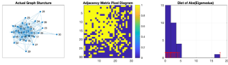
Figure 2: A random graph instance with 30 nodes generated following the uniform attachment procedure, its pixel representation and the distribution of modulus of the eigenvalues.

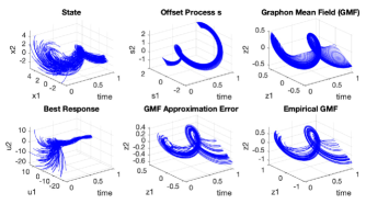
Figure 3: Simulations on the uniform attachment graph example in Fig. 2 with 30 nodes where each node contains $4$ agents and each agent has $2$ states.

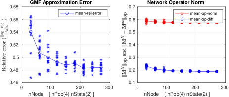
Figure 4: The relative error in the graphon mean field decreases as graph sizes increase. 12 simulation independent experiments are carried out for each size. The nodal population size denoted by nPop is $4$, the local state dimension denoted by nState is 2. In the figure on the right, black dots represent the values for $\|\mathbf{M^{[N]}}-\mathbf{M}\|_{\textup{op}}$ in different simulation experiments.

The parameters in the simulations are:

$$A=\begin{bmatrix}0&10\\ -10&0\end{bmatrix},~{}Q=\begin{bmatrix}0.5&0\\ 0&0.5\end{bmatrix},~{}\Sigma=\begin{bmatrix}0.1&0\\ 0&0.1\end{bmatrix},$$ (82)

$$B=D=R=Q_{T}=\begin{bmatrix}1&0\\ 0&1\end{bmatrix},~{}\eta=\begin{bmatrix}2\\ 2\end{bmatrix},~{}H=\begin{bmatrix}1&0\\ 0&1\end{bmatrix},$$

$$~{}T=1,n=2,~{}N=30,~{}|C_{\ell}|=4,~{}1\leq\ell\leq N.$$

The graphon limit is approximated by the 5 most signification eigen directions. We observe that the approximation by the 5 most significant eigen directions of $\mathbf{M}$ has less than $1\%$ relative error in terms of the operator norm. The initial conditions are independently generated from Gaussian distributions with variance $1$ and means that are sampled from a uniform distribution in $[-3,3]$. These means are used in computing the approximate graphon mean field game solutions. In the example in Fig. 2 and Fig. 3, the graphon mean field approximation relative error $\frac{\|\mathbf{z}_{E}-\mathbf{z}\|_{C}}{\|\mathbf{z}_{E}\|_{C}}$ is $52.569\%$ where $\mathbf{z}_{E}$ is the actual network mean field and $\mathbf{z}$ is the graphon mean field computed based on the Global LQG-GMFG Forward-Backward Equations. The error between the graphon limit $\mathbf{M}$ and the step function graphon $\mathbf{M^{[N]}}$ (associated with the 30-node graph in Fig. 2) is $\|\mathbf{M}-\mathbf{M^{[N]}}\|_{\textup{op}}=0.238$ and the graphon limit operator norm is $\|\mathbf{M}\|_{\textup{op}}=0.386$. The relative approximation errors decrease as the sizes of the graphs increase, which is numerically illustrated by a set of examples for graphs with different sizes in Fig. 4.

VIII-B Example 2: Stochastic Block Models (SBM)

VIII-B1 Random Graphs Generated from SBM and Properties

Following [7, p.157], random simple graphs with $N$ nodes can be generated from a graphon $\mathbf{M}$ by first sampling data points $x_{1},...,x_{N}$ from the uniform distribution on $[0,1]$ and then connecting node $i$ and node $j$ with probability $\mathbf{M}(x_{i},x_{j})$, for all $i,j\in\{1,...,N\}$ and $i\neq j$. Stochastic block models can be approximately considered as models of generating $\mathbf{M}$-random graphs where the graphon $\mathbf{M}$ is a step function graphon (see [46]). Consider the stochastic block model matrix $W=[w_{ij}]\in\mathds{R}^{d\times d}$. The associated graphon limit is given by $\mathbf{M}(x,y)=\sum_{i=1}^{d}\sum_{j=1}^{d}w_{ij}\mathds{1}_{P_{i}}(x)\mathds{1}_{P_{j}}(y),~{}(x,y)\in[0,1]^{2}$ with the uniform partition $\{P_{1},....,P_{d}\}$ of $[0,1]$. Denote the eigen decomposition $W=\sum_{\ell=1}^{d}\lambda_{\ell}v_{\ell}v_{\ell}^{\mathchoice{\raisebox{0.0pt}{$\displaystyle\intercal$}}{\raisebox{0.0pt}{$\textstyle\intercal$}}{\raisebox{0.0pt}{$\scriptstyle\intercal$}}{\raisebox{0.0pt}{$\scriptscriptstyle\intercal$}}}$ where $\{\lambda_{\ell}\}$ are the eigenvalues (allowing repeated eigenvalues) and $\{v_{\ell}\}$ are the associated normalized eigenvectors. Then the spectral decomposition of the associated graphon is given by $\mathbf{M}(x,y)=\sum_{\ell=1}^{d}\frac{\lambda_{\ell}}{d}\mathbf{v}_{\ell}(x)\mathbf{v}_{\ell}(y),~{}(x,y)\in[0,1]^{2}$ where $\mathbf{v}^{\ell}(x)=\sum_{i=1}^{d}\mathds{1}_{P_{i}}(x)v_{\ell}(i)$ (see also [16]). The graphon is a step function and hence obviously a low-rank graphon with the same number of non-zero eigenvalues as that of the block matrix $W$.

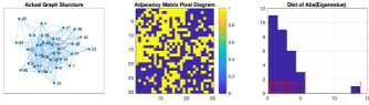
Figure 5: A graph generated from SBM, its pixel diagram and the distribution of the modulus of eigenvalues.

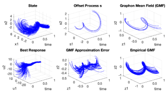
Figure 6: Simulation on a network generated from SBM with 30 nodes where each node contains 4 agents and each agent has 2 states.

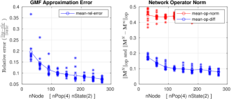
Figure 7: Graphon mean field game approximation errors on networks of different sizes. $12$ simulations are carried out for each size. The nodal population size denoted by nPop is $4$, and the local state dimension denoted by nState is $2$. In the figure on the right, black dots represent values for $\|\mathbf{M^{[N]}}-\mathbf{M}\|_{\textup{op}}$ in different simulation experiments.

VIII-B2 Simulations on Random Graphs Generated from SBM

The parameters in the simulation are the same as those in (82). The initial conditions are independently drawn from Gaussian distributions with variance $1$ and mean values that are generated randomly from $[-3,3]$. These mean values are used in computing the approximate graphon mean field game solutions. The block matrix of SBM is given by

$$W=\begin{bmatrix}0.25&0.5&0.2\\ 0.5&0.35&0.7\\ 0.2&0.7&0.4\end{bmatrix}.$$ (83)

The simulation result on the graph instance in Fig. 5 which is generated from the SBM with matrix (83) is illustrated in Fig. 6. For this particular example, the graphon mean field relative approximation error $\frac{\|\mathbf{z}_{E}-\mathbf{z}\|_{C}}{\|\mathbf{z}_{E}\|_{C}}$ is $29.256\%$ where $\mathbf{z}_{E}$ is the actual network mean field and $\mathbf{z}$ is the graphon mean field computed based on the Global LQG-GMFG Forward-Backward Equations. The error between the graphon limit $\mathbf{M}$ and the step function graphon $\mathbf{M^{[N]}}$ (associated with the graph) is $\|\mathbf{M}-\mathbf{M^{[N]}}\|_{\textup{op}}=0.178$ and the graphon limit operator norm is $\|\mathbf{M}\|=0.434$. The relative approximation error $\frac{\|\mathbf{z}_{E}-\mathbf{z}\|_{C}}{\|\mathbf{z}_{E}\|_{C}}$ decreases as the size of the network increases as illustrated by results on graphs of different sizes in Fig. 7.

IX Conclusion

This work studied solution methods for LQG graphon mean field game problems based on subspace and spectral decompositions. Future work should focus on cases with heterogeneous parameters in dynamics, computational procedures for nonlinear graphon mean field games, graphon control for nonlinear systems, and the counterpart theory for sparse graphs.

Appendix A Proof of Proposition 8

Proof

To explicitly verify the eigen pairs of $\mathbf{M}$, we have the following computation. Let $\mathbf{v}_{k}=\cos\left(\frac{\pi k\beta}{2}\right),k\in\{1,3,5,...\}$. Then for any $\alpha\in[0,1]$ and any $k\in\{1,3,5,...\}$, the following holds

$$[\mathbf{M}\mathbf{v}_{k}](\alpha)=\int_{0}^{1}(1-\max(\alpha,\beta))\cos\big{(}\frac{\pi k\beta}{2}\big{)}d\beta$$

$$=\int_{0}^{1}\cos\big{(}\frac{\pi k\beta}{2}\big{)}d\beta-\int_{0}^{\alpha}\alpha\cos\big{(}\frac{\pi k\beta}{2}\big{)}d\beta$$

$$~{}-\int_{\alpha}^{1}\beta\cos\big{(}\frac{\pi k\beta}{2}\big{)}d\beta=\frac{4}{k^{2}\pi^{2}}\cos\big{(}\frac{\pi k\alpha}{2}\big{)}=\frac{4}{k^{2}\pi^{2}}\mathbf{v}_{k}(\alpha).$$

To verify that all the eigen pairs are listed, one can simply check the relation between the sum of squares of the eigenvalues and the 2-norm. First, we compute $\sum_{\ell=1}\lambda_{\ell}^{2}=\left(\frac{4}{\pi^{2}}\right)^{2}\sum_{k=0}^{\infty}\frac{1}{(2k+1)^{4}}=\frac{1}{6}.$ Second, we compute $\|\mathbf{M}\|_{2}^{2}=\int_{[0,1]}\int_{[0,1]}(1-\max(x,y))^{2}dxdy=\frac{1}{6}.$ Therefore, the equality $\|\mathbf{M}\|_{2}^{2}=\sum_{\ell=1}\lambda_{\ell}^{2}$ is satisfied, which implies we have listed all the eigenpairs in (80). Hence the spectral decomposition of the uniform attachement graphon limit is then given by (81).

Appendix B Computing Solutions to Joint Equations

This section contains two numerical algorithms to solve the joint forward backward equations (19) and (20). With spectral approximations of the graphon limit, these algorithms can provide approximate numerical solutions to the Global LQG-GMFG Forward-Backward Equations (28) and (29). If, furthermore, the underlying graphon is of finite rank, then these algorithms provide exact numerical solutions to the Global LQG-GMFG Forward-Backward Equations (28) and (29) given an appropriate choice of basis functions for the characterizing finite dimensional subspace.

Algorithm 1 Solving joint forward backward equations based on fixed point iterations.

0:  Initial condition $z_{0}$, equation parameters $A$, $B$, $D$, $M$, $Q$, $Q_{T}$, $R$, $n$, $N$, $H$ and $\eta$, time horizon $T$, sampling period $dt$, maximum number of iterations ${nIteration}$, error tolerance $tol$.

0:  z, s, $\Delta$ Initialisation: $z$ process with $z(0)=z_{0}$

1:  $\Pi$ $\leftarrow$ $\Pi$-Dynamics($\Pi_{T}$, $T$, $dt$)

2:  for iteration $i=1,2...$ to $nIteration$ do

3:     $s$ $\leftarrow$ s-DynamicsIntegrateBackward($z$, $\Pi$, $T$, $dt$)

4:     $z^{+}$ $\leftarrow$ z-DynamicsIntegrateForward($s$, $\Pi$, $T$, $dt$)

5:     $\Delta$ = $\|z^{+}-z\|$

6:     Update $z\leftarrow z^{+}$

7:     if ($\Delta\leq tol$) then

8:        break

9:     end if

10:  end for

11:  return  $z$, $s$, $\Delta$.

Algorithm 2 Solving joint forward backward equations based on a decoupling Riccati equation.

0:  Initial condition $z(0)=z_{0}$, equation parameters $A$, $B$, $D$, $M$, $Q$, $Q_{T}$, $R$, $n$, $N$, $H$ and $\eta$, time horizon $T$, sampling period $dt$.

0:  $z$, $s$ Initialisation: $e(T)=(H\otimes Q_{T})(\mathbf{1_{n}}\otimes\eta)$,$P(T)=H\otimes Q_{T}$,

1:  $\Pi$ $\leftarrow$ $\Pi$-Dynamics($\Pi_{T}$, $T$, $dt$)

2:  $P$ $\leftarrow$ P-DynamicsIntegrateBackward($P(T)$, $\Pi$, $T$, $dt$)

3:  $e$ $\leftarrow$ e-DynamicsIntegrateBackward($e(T)$, $\Pi$, $T$, $dt$)

4:  $z$ $\leftarrow$ z-DynamicsIntegrateForward($z(0)$, $e$, $P$, $\Pi$, $T$, $dt$)

5:  $s(T)=Hz(T)+\mathbf{1}\otimes\eta$

6:  $s$ $\leftarrow$ s-DynamicsIntegrateBackward($s(T)$, $z$, $\Pi$, $T$, $dt$)

7:  return  $z$ and $s$.

For convenience, we list here the equations used in the algorithms. Let $A_{c}(t)\triangleq(A-BR^{-1}B^{\mathchoice{\raisebox{0.0pt}{$\displaystyle\intercal$}}{\raisebox{0.0pt}{$\textstyle\intercal$}}{\raisebox{0.0pt}{$\scriptstyle\intercal$}}{\raisebox{0.0pt}{$\scriptscriptstyle\intercal$}}}\Pi_{t})$ and $\mathbf{1}_{n}$ denote the $n$-dimensional vector of ones. $\Pi$-Dynamics refers to Eqn. (21).
P-Dynamics:

$$-\dot{\bar{P}}= (I_{N}\otimes A_{c}(t)^{\mathchoice{\raisebox{0.0pt}{$\displaystyle\intercal$}}{\raisebox{0.0pt}{$\textstyle\intercal$}}{\raisebox{0.0pt}{$\scriptstyle\intercal$}}{\raisebox{0.0pt}{$\scriptscriptstyle\intercal$}}})\bar{P}+\bar{P}(I_{N}\otimes A_{c}(t))$$

$$-\bar{P}\big{(}M_{\mathbf{f}}\otimes BR^{-1}B^{\mathchoice{\raisebox{0.0pt}{$\displaystyle\intercal$}}{\raisebox{0.0pt}{$\textstyle\intercal$}}{\raisebox{0.0pt}{$\scriptstyle\intercal$}}{\raisebox{0.0pt}{$\scriptscriptstyle\intercal$}}}\big{)}\bar{P}-(I_{N}\otimes(QH-\Pi_{t}D)),$$

$$\bar{P}(T) =I_{N}\otimes Q_{T}H.$$

s-Dynamics:

$$-\dot{\bar{s}}(t)= I_{{}_{N}}\otimes A_{c}(t)^{\mathchoice{\raisebox{0.0pt}{$\displaystyle\intercal$}}{\raisebox{0.0pt}{$\textstyle\intercal$}}{\raisebox{0.0pt}{$\scriptstyle\intercal$}}{\raisebox{0.0pt}{$\scriptscriptstyle\intercal$}}}\bar{s}(t)-I_{{}_{N}}\otimes(QH-\Pi_{t}D)\bar{z}(t)$$

$$~{}~{}-(I_{{}_{N}}\otimes{H}Q)(\mathbf{1}_{n}\otimes\eta)$$

$$\bar{s}(T)= (I_{N}\otimes Q_{T}H)(\bar{z}(T)+\mathbf{1}_{n}\otimes\eta).$$

z-Dynamics based on $s$:

$$\dot{\bar{z}}(t)= I_{{}_{N}}\otimes A_{c}(t)\bar{z}(t)+\frac{1}{N}M\otimes D\bar{z}(t)$$

$$-\frac{1}{N}M\otimes BR^{-1}B^{\mathchoice{\raisebox{0.0pt}{$\displaystyle\intercal$}}{\raisebox{0.0pt}{$\textstyle\intercal$}}{\raisebox{0.0pt}{$\scriptstyle\intercal$}}{\raisebox{0.0pt}{$\scriptscriptstyle\intercal$}}}\bar{s}(t),\quad\bar{z}(0)={\color[rgb]{0,0,0}\frac{1}{N}{(M\otimes I_{n})}}\bar{x}(0).$$

e-Dynamics:

$$\dot{e}(t) =\Big{(}-I_{{}_{N}}\otimes A_{c}(t)^{\mathchoice{\raisebox{0.0pt}{$\displaystyle\intercal$}}{\raisebox{0.0pt}{$\textstyle\intercal$}}{\raisebox{0.0pt}{$\scriptstyle\intercal$}}{\raisebox{0.0pt}{$\scriptscriptstyle\intercal$}}}+P(t)M\otimes BR^{-1}B^{\mathchoice{\raisebox{0.0pt}{$\displaystyle\intercal$}}{\raisebox{0.0pt}{$\textstyle\intercal$}}{\raisebox{0.0pt}{$\scriptstyle\intercal$}}{\raisebox{0.0pt}{$\scriptscriptstyle\intercal$}}}\Big{)}e(t)$$

$$\quad+(I_{N}\otimes QH)(\mathbf{1}_{n}\otimes\eta),~{}e(T)=I_{N}\otimes Q_{T}H(\mathbf{1}_{n}\otimes\eta).$$

z-Dynamics based on $P$ and $e$:

$$\dot{\bar{z}}(t) =\Big{(}I_{N}\otimes A_{c}(t)-[M\otimes BR^{-1}B^{\mathchoice{\raisebox{0.0pt}{$\displaystyle\intercal$}}{\raisebox{0.0pt}{$\textstyle\intercal$}}{\raisebox{0.0pt}{$\scriptstyle\intercal$}}{\raisebox{0.0pt}{$\scriptscriptstyle\intercal$}}}]P(t)+M\otimes D\Big{)}\bar{z}(t)$$

$$~{}~{}\quad{-}\big{(}M\otimes BR^{-1}B^{\mathchoice{\raisebox{0.0pt}{$\displaystyle\intercal$}}{\raisebox{0.0pt}{$\textstyle\intercal$}}{\raisebox{0.0pt}{$\scriptstyle\intercal$}}{\raisebox{0.0pt}{$\scriptscriptstyle\intercal$}}}\big{)}e(t),\quad\bar{z}(0)={\color[rgb]{0,0,0}\frac{1}{N}}{(M\otimes I_{n})}\bar{x}(0).$$

These equations are solved using ode45 in MATLAB. Then the trajectories of the solutions are sampled with sampling period $dt$. Such sampled trajectories are then interpolated using piecewise cubic Hermite interpolating polynomials (pchip) and used in fixed point iterations and in the computation of time-dependent differential equations.

Shuang Gao (S’14-M’19) received the B.E. degree in automation and M.S. in control science and engineering, from Harbin Institute of Technology, Harbin, China, in 2011 and 2013. He received the Ph.D. degree in electrical engineering from McGill University, Montreal, QC, Canada, in February 2019, under the supervision of Prof. Peter. E. Caines. He is currently a Postdoctoral Researcher at the Department of Electrical and Computer Engineering at McGill University. He is a member of McGill Centre for Intelligent Machines and Groupe d’Études et de Recherche en Analyse des Décisions. His research interest includes control of network systems, optimization on networks, network modelling, mean field games.

Peter E. Caines (LF’11) received the BA in mathematics from Oxford University in 1967 and the PhD in systems and control theory in 1970 from Imperial College, University of London, under the supervision of David Q. Mayne, FRS. After periods as a postdoctoral researcher and faculty member at UMIST, Stanford, UC Berkeley, Toronto and Harvard, he joined McGill University, Montreal, in 1980, where he is Distinguished James McGill Professor and Macdonald Chair in the Department of Electrical and Computer Engineering. In 2000 the adaptive control paper he coauthored with G. C. Goodwin and P. J. Ramadge (IEEE Transactions on Automatic Control, 1980) was recognized by the IEEE Control Systems Society as one of the 25 seminal control theory papers of the 20th century. In 2009 Peter Caines received the IEEE Control Systems Society Bode Lecture Prize. He is a Life Fellow of the IEEE, and a Fellow of SIAM, IFAC, the Institute of Mathematics and its Applications (UK) and the Canadian Institute for Advanced Research and is a member of Professional Engineers Ontario. He was elected to the Royal Society of Canada in 2003. Peter Caines is the author of Linear Stochastic Systems, John Wiley, 1988, republished as a SIAM Classic in 2018, and is a Senior Editor of Nonlinear Analysis-Hybrid Systems; his research interests include stochastic, mean field game, decentralized and hybrid systems theory, together with their applications in a range of fields.

Minyi Huang (S’01-M’04) received the B.Sc. degree from Shandong University, Jinan, Shandong, China, in 1995, the M.Sc. degree from the Institute of Systems Science, Chinese Academy of Sciences, Beijing, in 1998, and the Ph.D. degree from the Department of Electrical and Computer Engineering, McGill University, Montreal, QC, Canada, in 2003, all in systems and control. He was a Research Fellow first in the Department of Electrical and Electronic Engineering, the University of Melbourne, Melbourne, Australia, from February 2004 to March 2006, and then in the Department of Information Engineering, Research School of Information Sciences and Engineering, the Australian National University, Canberra, from April 2006 to June 2007. He joined the School of Mathematics and Statistics, Carleton University, Ottawa, ON, Canada as an Assistant Professor in July 2007, where he is now a Professor. His research interests include mean field stochastic control and dynamic games, multi-agent control and computation in distributed networks with applications.

Appendix C Convergence Analysis

Let $(\mathbf{z^{[N]}},\mathbf{s^{[N]}})$ denote the solution pair to (26) and (27) and let $(\mathbf{z},\mathbf{s})$ denote the solution pair to (28) and (29). Let $z_{{}_{E}}\triangleq\{z_{{}_{E}}(t)\in\mathds{R}^{nN}:t\in[0,T]\}$ denote the actual network empirical average vector on an $N$-node graph with nodal population sizes $\{|\mathcal{C}_{q}|:q\in\mathcal{V}_{c}\}$ when the graphon mean field game solution (32) is implemented by all agents. Let $\mathbf{z}_{E}^{\mathbf{N}}$ denote the piece-wise constant function (in the space variable) in $C([0,T];(L^{2}_{pwc}[0,1])^{n})$ associated with $z_{{}_{E}}$.

C-A Network Mean Field to Graphon Mean Field

Theorem 2 (Finite Network MF to Graphon MF)

If there exists a constant $c_{0}$ ($0\leq c_{0}<1$) such that

$$\textup{L}_{0}(\mathbf{M})\leq c_{0}\quad\text{ and }\quad\textup{L}_{0}(\mathbf{M^{[N]}})\leq c_{0}~{}\text{for all $N$},$$ (84)

then there exists a unique classical solution pair $(\mathbf{z^{[N]}},\mathbf{s^{[N]}})$ to the joint equations (26) and (27) for each $N$ and a unique classical solution pair $(\mathbf{z},\mathbf{s})$ to the joint equations (28) and (29). If, furthermore,

$$\lim_{N\to\infty}\|\mathbf{M}-\mathbf{M^{[N]}}\|_{\textup{op}}=0,~{}\textup{and}~{}\lim_{N\to\infty}\|\mathbf{z}(0)-\mathbf{z^{[N]}}(0)\|_{2}=0,$$ (85)

then

$$\lim_{N\to\infty}\|\mathbf{s}-\mathbf{s^{[N]}}\|_{C}=0~{}~{}\textup{and}~{}~{}\lim_{N\to\infty}\|\mathbf{z}-\mathbf{z^{[N]}}\|_{C}=0,$$ (86)

and the asymptotic error for $\|\mathbf{z}-\mathbf{z^{[N]}}\|_{{}_{C}}$ and that for $\|\mathbf{s}-\mathbf{s^{[N]}}\|_{{}_{C}}$ are given by

$$O\left\{\max(\|\mathbf{M}-\mathbf{M^{[N]}}\|_{\textup{op}},~{}\|\mathbf{z}(0)-\mathbf{z^{[N]}}(0)\|_{2})\right\}.$$ (87)

C-B Proof for Theorem 2

To prove Theorem 2 we introduce the following lemma.

Lemma 9

The following holds for all $\tau,t\in[0,T]$ and for all $\mathbf{v}\in(L^{2}[0,1])^{n}$ :

$$\|(\phi_{1}^{\mathbf{M}}(t,\tau)-\phi_{1}^{\mathbf{M^{[N]}}}(t,\tau))\mathbf{v}\|_{2}\leq c_{1}(N)\|\mathbf{M}-\mathbf{M^{[N]}}\|_{\textup{op}}\|\mathbf{v}\|_{2}$$ (88)

where $\phi_{1}^{\mathbf{M}}(\cdot,\cdot)$ and $\phi_{1}^{\mathbf{M^{[N]}}}(\cdot,\cdot)$ denote the evolution operators respectively associated with $[\mathbb{A}(\cdot)+D\mathbf{M}]$ and $[\mathbb{A}(\cdot)+D\mathbf{M^{[N]}}]$,

$$c_{1}(N)\triangleq\|D\|_{2}\sup_{t,\tau\in[0,T]}$$ (89)

$$\Big{\{}\exp\Big{(}\int_{\tau}^{t}\big{\|}[\mathbb{A}(q)+D\mathbf{M^{[N]}}]\big{\|}_{\textup{op}}dq\Big{)}\int_{\tau}^{t}\|\phi_{1}^{\mathbf{M}}(q,\tau)\|_{\textup{op}}dq\Big{\}}$$

and $\|D\|_{2}$ denotes the matrix 2-norm (i.e., the maximum singular value of $D$). Furthermore, if there exists $\mathbf{M}\in\mathcal{W}_{c}$ such that $\lim_{N\to\infty}\|\mathbf{M}-\mathbf{M^{[N]}}\|_{\textup{op}}=0,$ then there exists a constant $c_{1}>0$ such that $c_{1}(N)\leq c_{1}$ holds uniformly in $N$.

Proof

Recall that $\Phi_{1}^{\mathbf{M}}(\cdot,\cdot)$ and $\Phi_{1}^{\mathbf{M^{[N]}}}(\cdot,\cdot)$ satisfy

$$\frac{\partial\phi_{1}^{\mathbf{M}}(t,\tau)}{\partial t} =[\mathbb{A}(t)+D\mathbf{M}]\phi_{1}^{\mathbf{M}}(t,\tau),~{}\phi_{1}^{\mathbf{M}}(\tau,\tau)=\mathbb{I},$$

$$\frac{\partial\phi_{1}^{\mathbf{M^{[N]}}}(t,\tau)}{\partial t} =[\mathbb{A}(t)+D\mathbf{M^{[N]}}]\phi_{1}^{\mathbf{M^{[N]}}}(t,\tau),$$

$$~{}\phi_{1}^{\mathbf{M^{[N]}}}(\tau,\tau) =\mathbb{I},\quad\forall\tau,t\in[0,T],$$

where $\mathbb{A}(t)\triangleq[(A-BR^{-1}B^{\mathchoice{\raisebox{0.0pt}{$\displaystyle\intercal$}}{\raisebox{0.0pt}{$\textstyle\intercal$}}{\raisebox{0.0pt}{$\scriptstyle\intercal$}}{\raisebox{0.0pt}{$\scriptscriptstyle\intercal$}}}\Pi_{t})\mathbb{I}]$. Let $\Delta(t,\tau)\triangleq\phi_{1}^{\mathbf{M^{[N]}}}(t,\tau)-\phi_{1}^{\mathbf{M}}(t,\tau)\in\mathcal{L}\big{(}(L^{2}[0,1])^{n}\big{)}$ for $t,\tau\in[0,T]$. The evolution of $\Delta(\cdot,\cdot)$ satisfies

$$\frac{\partial\Delta(t,\tau)}{\partial t}= [\mathbb{A}(t)+D\mathbf{M^{[N]}}]\Delta(t,\tau)$$ (90)

$$+[D(\mathbf{M^{[N]}}-\mathbf{M})]\phi_{1}^{\mathbf{M}}(t,\tau),$$

with initial conditions $\Delta(\tau,\tau)=0\in\mathcal{L}\big{(}(L^{2}[0,1])^{n}\big{)}$ for all $t,\tau\in[0,T]$. Therefore, for all $\mathbf{v}\in(L^{2}[0,1])^{n}$,

$$\Delta(t,\tau)\mathbf{v}= \int_{\tau}^{t}[\mathbb{A}(q)+D\mathbf{M^{[N]}}]\Delta(q,\tau)\mathbf{v}dq$$ (91)

$$\quad+[D(\mathbf{M^{[N]}}-\mathbf{M})]\int_{\tau}^{t}\phi_{1}^{\mathbf{M}}(q,\tau)\mathbf{v}dq.$$

Hence the following inequality holds: for all $\mathbf{v}\in(L^{2}[0,1])^{n}$,

$$\|\Delta(t,\tau) \mathbf{v}\|_{2}\leq\int_{\tau}^{t}\big{\|}[\mathbb{A}(q)+D\mathbf{M^{[N]}}]\big{\|}_{\textup{op}}\|\Delta(q,\tau)\mathbf{v}\|_{2}dq$$

$$+\big{\|}[D(\mathbf{M^{[N]}}-\mathbf{M})]\big{\|}_{\textup{op}}\int_{\tau}^{t}\|\phi_{1}^{\mathbf{M}}(q,\tau)\mathbf{v}\|_{2}dq.$$

Then by the Grönwall-Bellman inequality, we obtain

$$\|\Delta(t,\tau) \mathbf{v}\|_{2}\leq\exp\Big{(}\int_{\tau}^{t}\big{\|}[\mathbb{A}(q)+D\mathbf{M^{[N]}}]\big{\|}_{\textup{op}}dq\Big{)}$$

$$\cdot\int_{\tau}^{t}\big{\|}[D(\mathbf{M^{[N]}}-\mathbf{M})]\big{\|}_{\textup{op}}\|\phi_{1}^{\mathbf{M}}(q,\tau)\|_{\textup{op}}\|\mathbf{v}\|_{2}dq,$$

for all $\mathbf{v}\in(L^{2}[0,1])^{n}$, which implies (88).

Clearly, for any $\mathbf{M}\in\mathcal{W}_{c}$, $\|\mathbf{M}\|_{\textup{op}}\leq\|\mathbf{M}\|_{2}$ is finite. If there exists $\mathbf{M}\in\mathcal{W}_{c}$ such that $\lim_{N\to\infty}\|\mathbf{M}-\mathbf{M^{[N]}}\|_{\textup{op}}=0,$ then one can verify that $\{\|\mathbf{M^{[N]}}\|_{\textup{op}}\}$ is uniformly bounded in $N$, and based on the definition of $c_{1}(N)$ in (89), this implies $c_{1}(N)$ is uniformly bounded in $N$.

We proceed to prove Theorem 2 in the following.

Proof

An application of Lemma 4 yields the existence of a unique classical solution pair $(\mathbf{z},\mathbf{s})$ and that of $(\mathbf{z^{[N]}},\mathbf{s^{[N]}})$.

Let the operation $\Gamma(\cdot):(L^{2}[0,1])^{n}\to(L^{2}[0,1])^{n}$ in (35) be associated with $\mathbf{M}$ and initial condition $\mathbf{z}(0)$; similarly let $\Gamma_{\mathbf{N}}(\cdot):(L^{2}[0,1])^{n}\to(L^{2}[0,1])^{n}$ denote the operator in (35) with $\mathbf{M}$ replaced by $\mathbf{M^{[N]}}$ and with $\mathbf{z}(0)$ replaced by $\mathbf{z^{[N]}}(0)$, that is

$$( \Gamma_{\mathbf{N}}(\mathbf{v}))(t)$$ (92)

$$\triangleq\phi_{1}^{\mathbf{M^{[N]}}}(t,0)\mathbf{z}^{\mathbf{N}}(0)-\int_{0}^{t}\phi_{1}^{\mathbf{M^{[N]}}}(t,\tau)[BR^{-1}B^{\mathchoice{\raisebox{0.0pt}{$\displaystyle\intercal$}}{\raisebox{0.0pt}{$\textstyle\intercal$}}{\raisebox{0.0pt}{$\scriptstyle\intercal$}}{\raisebox{0.0pt}{$\scriptscriptstyle\intercal$}}}\mathbf{M^{[N]}}]$$

$$\quad\Big{\{}\phi_{2}(\tau,T)[Q_{T}H\mathbb{I}](\mathbf{v}(T)+\eta\mathbf{1})-$$

$$\int^{T}_{\tau}\phi_{2}(\tau,q)\big{(}[(QH-\Pi_{q}D)\mathbb{I}]\mathbf{v}(q)+[QH\mathbb{I}]\eta\mathbf{1}\big{)}dq\Big{\}}d\tau.$$

By Lemma 4 we obtain that under the assumptions in (84) there exists a unique fixed point $\mathbf{v}^{*}$ (resp. $\mathbf{v}_{\mathbf{N}}^{*}$) for $\Gamma(\cdot)$ (resp. $\Gamma_{\mathbf{N}}(\cdot)$), that is, $\Gamma(\mathbf{v}^{*})=\mathbf{v}^{*}~{}\text{and}~{}\Gamma_{\mathbf{N}}(\mathbf{v}^{*}_{\mathbf{N}})=\mathbf{v}^{*}_{\mathbf{N}}.$ Firstly, by the triangle inequality,

$$\|\Gamma(\mathbf{v}^{*}) -\Gamma_{\mathbf{N}}(\mathbf{v}^{*}_{\mathbf{N}})\|_{C}$$ (93)

$$\leq\|\Gamma(\mathbf{v}^{*})-\Gamma_{\mathbf{N}}(\mathbf{v}^{*})\|_{C}+\|\Gamma_{\mathbf{N}}(\mathbf{v}^{*})-\Gamma_{\mathbf{N}}(\mathbf{v}^{*}_{\mathbf{N}})\|_{C}.$$

Following the definitions of $\Gamma(\cdot)$ and $\Gamma_{\mathbf{N}}(\cdot)$, we know

$$\|\Gamma(\mathbf{v}^{*})(t)-\Gamma_{\mathbf{N}}(\mathbf{v}^{*})(t)\|_{2}$$ (94)

$$\leq\left\|\phi_{1}^{\mathbf{M}}(t,0)\mathbf{z}(0)-\phi_{1}^{\mathbf{M^{[N]}}}\mathbf{z^{[N]}}(0))\right\|_{2}+\int_{0}^{t}$$

$$\Big{\|}\big{\{}\phi_{1}^{\mathbf{M}}(t,\tau)[BR^{-1}B^{\mathchoice{\raisebox{0.0pt}{$\displaystyle\intercal$}}{\raisebox{0.0pt}{$\textstyle\intercal$}}{\raisebox{0.0pt}{$\scriptstyle\intercal$}}{\raisebox{0.0pt}{$\scriptscriptstyle\intercal$}}}\mathbf{M}]-\phi_{1}^{\mathbf{M^{[N]}}}(t,\tau)[BR^{-1}B^{\mathchoice{\raisebox{0.0pt}{$\displaystyle\intercal$}}{\raisebox{0.0pt}{$\textstyle\intercal$}}{\raisebox{0.0pt}{$\scriptstyle\intercal$}}{\raisebox{0.0pt}{$\scriptscriptstyle\intercal$}}}\mathbf{M^{[N]}}]\big{\}}$$

$$\qquad\mathbf{y}(\tau,\mathbf{v}^{*})\Big{\|}_{2}d\tau\triangleq I_{1}(t)+\int_{0}^{t}I_{2}(t,\tau)d\tau,$$

for any $t\in[0,T]$, where

$$\mathbf{y}(\tau,\mathbf{v}^{*})\triangleq\Big{\{}\phi_{2}(\tau,T)[Q_{T}H\mathbb{I}](\mathbf{v}^{*}(T)+\eta\mathbf{1})-$$ (95)

$$~{}\int^{T}_{\tau}\phi_{2}(\tau,q)\big{(}[(QH-\Pi_{q}D)\mathbb{I}]\mathbf{v}^{*}(q)+[QH\mathbb{I}]\eta\mathbf{1}\big{)}dq\Big{\}}.$$

By Lemma 9 and the triangle inequality we obtain

$$I_{1}(t) \leq\left\|\phi_{1}^{\mathbf{M}}(t,0)\right\|_{\textup{op}}\left\|(\mathbf{z}(0)-\mathbf{z^{[N]}}(0))\right\|_{2}$$ (96)

$$\quad+c_{1}(N)\|(\mathbf{M^{[N]}}-\mathbf{M})\|_{\textup{op}}\|\mathbf{z^{[N]}}(0)\|_{2}.$$

Moreover, the second part of the right-hand side of equation (94) satisfies the following inequalities

$$I_{2}(t,\tau)\leq\left\|\big{\{}\phi_{1}^{\mathbf{M}}(t,\tau)[BR^{-1}B^{\mathchoice{\raisebox{0.0pt}{$\displaystyle\intercal$}}{\raisebox{0.0pt}{$\textstyle\intercal$}}{\raisebox{0.0pt}{$\scriptstyle\intercal$}}{\raisebox{0.0pt}{$\scriptscriptstyle\intercal$}}}(\mathbf{M}-\mathbf{M^{[N]}})]\right\|_{\textup{op}}\|\mathbf{y}(\tau,\mathbf{v}^{*})\|_{2}$$ (97)

$$+\Big{\|}\phi_{1}^{\mathbf{M}}(t,\tau)-\phi_{1}^{\mathbf{M^{[N]}}}(t,\tau)\Big{\|}_{\textup{op}}\|[BR^{-1}B^{\mathchoice{\raisebox{0.0pt}{$\displaystyle\intercal$}}{\raisebox{0.0pt}{$\textstyle\intercal$}}{\raisebox{0.0pt}{$\scriptstyle\intercal$}}{\raisebox{0.0pt}{$\scriptscriptstyle\intercal$}}}\mathbf{M^{[N]}}]\mathbf{y}(\tau,\mathbf{v}^{*})\|_{2}$$

$$\leq\|\mathbf{M}-\mathbf{M^{[N]}}\|_{\textup{op}}\lambda_{\max}(BR^{-1}B^{\mathchoice{\raisebox{0.0pt}{$\displaystyle\intercal$}}{\raisebox{0.0pt}{$\textstyle\intercal$}}{\raisebox{0.0pt}{$\scriptstyle\intercal$}}{\raisebox{0.0pt}{$\scriptscriptstyle\intercal$}}})c_{4}\Big{(}c_{3}+c_{1}(N)\|\mathbf{M^{[N]}}\|_{\textup{op}}\Big{)}$$

where

$$c_{3}\triangleq\sup_{t,\tau\in[0,T]}\|\phi_{1}^{\mathbf{M}}(t,\tau)\|_{\textup{op}},~{}~{}c_{4}\triangleq\sup_{\tau\in[0,T]}\|\mathbf{y}(\tau,\mathbf{v}^{*})\|_{2}.$$ (98)

We note that since $R>0$, the eigenvalues of $BR^{-1}B^{\mathchoice{\raisebox{0.0pt}{$\displaystyle\intercal$}}{\raisebox{0.0pt}{$\textstyle\intercal$}}{\raisebox{0.0pt}{$\scriptstyle\intercal$}}{\raisebox{0.0pt}{$\scriptscriptstyle\intercal$}}}$ are all non-negative real numbers. Let

$$c_{5}\triangleq\sup_{N}\|\mathbf{M^{[N]}}\|_{\textup{op}}\quad\text{and}\quad c_{6}\triangleq\sup_{N}\|\mathbf{z^{[N]}}(0)\|_{2}.$$

It can be verified that $c_{5}$ and $c_{6}$ (which are uniformly bounded in $N$) exist under the convergence assumptions in (85). Then by (94), (96) and (97), we obtain

$$\|\Gamma(\mathbf{v}^{*})(t)-\Gamma_{\mathbf{N}}(\mathbf{v}^{*})(t)\|_{2}$$ (99)

$$\leq c_{3}\left\|(\mathbf{z}(0)-\mathbf{z^{[N]}}(0))\right\|_{2}+c_{1}(N)\|(\mathbf{M^{[N]}}-\mathbf{M})\|_{\textup{op}}$$

$$\quad\cdot\Big{\{}c_{6}+c_{4}t\lambda_{\max}(BR^{-1}B)\Big{(}c_{3}+c_{1}(N)c_{5}\Big{)}\Big{\}}.$$

Secondly, following the definition of $\Gamma_{\mathbf{N}}(\cdot)$, we know that, under the assumptions in (84), for all $t\in[0,T]$,

$$\|\Gamma_{\mathbf{N}}(\mathbf{v}^{*})(t)-\Gamma_{\mathbf{N}}(\mathbf{v}^{*}_{\mathbf{N}})(t)\|_{2} \leq\textup{L}_{0}(\mathbf{M^{[N]}})\|\mathbf{v}^{*}-\mathbf{v}_{\mathbf{N}}^{*}\|_{C}$$ (100)

$$\leq c_{0}\|\mathbf{v}^{*}-\mathbf{v}_{\mathbf{N}}^{*}\|_{C}.$$

Therefore based on (93), (99) and (100), we yield

$$\|\mathbf{v}^{*}-\mathbf{v}^{*}_{\mathbf{N}}\|_{C} \leq c_{3}\left\|(\mathbf{z}(0)-\mathbf{z^{[N]}}(0))\right\|_{2}$$

$$+\Big{\{}c_{6}+c_{4}T\lambda_{\max}(BR^{-1}B)\Big{(}c_{3}+c_{1}(N)c_{5}\Big{)}\Big{\}}$$

$$+c_{0}\|\mathbf{v}^{*}-\mathbf{v}^{*}_{\mathbf{N}}\|_{C},$$

which then leads to the following upper bound

$$\|\mathbf{v}^{*}-\mathbf{v}^{*}_{\mathbf{N}}\|_{C}$$ (101)

$$\leq\frac{1}{1-c_{0}}\Bigg{\{}c_{3}\left\|(\mathbf{z}(0)-\mathbf{z^{[N]}}(0))\right\|_{2}+c_{1}(N)\|(\mathbf{M^{[N]}}-\mathbf{M})\|_{\textup{op}}$$

$$\qquad\qquad\quad\cdot\Big{[}c_{6}+c_{4}T\lambda_{\max}(BR^{-1}B)\Big{(}c_{3}+c_{1}(N)c_{5}\Big{)}\Big{]}\Bigg{\}},$$

with $0\leq c_{0}<1$. Since $c_{0}$, $c_{3}$, $c_{4}$, $c_{5}$ and $c_{6}$ do not depend on $N$, and $c_{1}(N)$ is uniformly bounded for all $N$ by Lemma 9, we yield that

$$\lim_{N\to\infty}\|\mathbf{v}^{*}-\mathbf{v}^{*}_{\mathbf{N}}\|_{C}=0.$$ (102)

Since the fixed point for $\Gamma(\cdot)$ is unique, clearly $\mathbf{v}^{*}$ is exactly the $\mathbf{z}$ part of the classical solution pair $(\mathbf{z},\mathbf{s})$ to (28) and (29), and $\mathbf{v}_{\mathbf{N}}^{*}$ is exactly the solution $\mathbf{z^{[N]}}$ part of the solution pair $(\mathbf{z^{[N]}},\mathbf{s^{[N]}})$ to (26) and (27). Hence the above equations (102) and (101), together with relationship between $\mathbf{s}$ and $\mathbf{z}$ in (34), imply (86) and (87).

We note that in general the error bounds depend on the time horizon $T$ as well. Since we formulate the problems with a fixed time horizon $T$, the time dependence will not be shown explicitly in the statement of Theorem 2.

C-C Network Empirical Average to Graphon Mean Field

The graphon mean field which is used to generate LQG-GMFG strategies for agents provides an approximation of the actual network empirical average. In the following we provide an asymptotic bound for this approximation error.

Theorem 3 (Network Empirical Average to Graphon MF)

Assume the distribution of random initial conditions at node $q\in\mathcal{V}_{c}$ has mean $\mu_{q}$ and finite variance uniformly bounded with respect to $|\mathcal{V}_{c}|$ and $|\mathcal{C}_{q}|$. Let $\mathbf{z^{[N]}}(0)$ in $(L^{2}_{pwc}[0,1])^{n}$ denote the piece-wise constant function associated with the initial condition of the network mean field $\bar{z}(0)=\frac{1}{N}M[\mu_{1},....,\mu_{N}]^{\mathchoice{\raisebox{0.0pt}{$\displaystyle\intercal$}}{\raisebox{0.0pt}{$\textstyle\intercal$}}{\raisebox{0.0pt}{$\scriptstyle\intercal$}}{\raisebox{0.0pt}{$\scriptscriptstyle\intercal$}}}$. Under the assumptions in (84) and (85), the asymptotic error in terms of the expected difference between the network empirical average $\mathbf{z}_{E}^{\mathbf{N}}$ and the graphon mean field $\mathbf{z}$ (after taking both the nodal population limit and the graphon limit) is given by

$$\mathbb{E}\|\mathbf{z}_{E}^{\mathbf{N}}-\mathbf{z}\|_{C}=O\Big{\{}\max\Big{(}\|\mathbf{M}-\mathbf{M^{[N]}}\|_{\textup{op}},$$ (103)

$$\qquad\qquad\qquad\quad~{}\|\mathbf{z}(0)-\mathbf{z^{[N]}}(0)\|_{2},~{}\frac{1}{\sqrt{\min_{q\in\mathcal{V}_{c}}|\mathcal{C}_{q}|}}\Big{)}\Big{\}},$$

where the expectation is taken with respect to the distributions of additive noises in the dynamics and random initial conditions.

Proof

Theorem 2 provides the difference between the graphon mean field $\mathbf{z}$ (after taking both the graphon limit and the nodal population limit) and the network mean field $\mathbf{z^{[N]}}$ (after taking only the nodal population limit). In order to analyze the difference between the network empirical average $\mathbf{z}^{\mathbf{N}}_{{}_{E}}$ and the graphon mean field $\mathbf{z}$, we need to find out the difference between the network mean field $\mathbf{z^{[N]}}$ and the network empirical average $\mathbf{z}^{\mathbf{N}}_{{}_{E}}$.

Recall from (12) the dynamics of agent $i\in\{1,...,K\}:$

$$dx_{i}(t)=(Ax_{i}(t)+Bu_{i}(t)+Dz_{i}(t))dt+\Sigma dw_{i}(t).$$ (104)

If the graph structure is exactly known to each agent, then based on Proposition 1, the network mean field strategy on the $N$-node graph is given by

$$u_{i}(t) =-R^{-1}B^{\mathchoice{\raisebox{0.0pt}{$\displaystyle\intercal$}}{\raisebox{0.0pt}{$\textstyle\intercal$}}{\raisebox{0.0pt}{$\scriptstyle\intercal$}}{\raisebox{0.0pt}{$\scriptscriptstyle\intercal$}}}(\Pi_{t}x_{i}(t)+\bar{s}_{q}(t)),\qquad i\in\mathcal{C}_{q}.$$ (105)

where $\bar{s}_{q}$ (if exists) is given by the solution pair $(\bar{s},\bar{z})$ to the joint equations (20) and (19), which is equivalently given by the solution pair $(\mathbf{s^{[N]}},\mathbf{z^{[N]}})$ to the step function graphon dynamical systems (26) and (27). Let $A_{c}(t)\triangleq(A-BR^{-1}B^{\mathchoice{\raisebox{0.0pt}{$\displaystyle\intercal$}}{\raisebox{0.0pt}{$\textstyle\intercal$}}{\raisebox{0.0pt}{$\scriptstyle\intercal$}}{\raisebox{0.0pt}{$\scriptscriptstyle\intercal$}}}\Pi_{t})$. Substituting the control in (104) by (105) yields the close-loop dynamics under network mean field strategy

$$dx_{i}(t) =A_{c}(t)x_{i}(t)+Dz_{i}(t)-BR^{-1}B^{\mathchoice{\raisebox{0.0pt}{$\displaystyle\intercal$}}{\raisebox{0.0pt}{$\textstyle\intercal$}}{\raisebox{0.0pt}{$\scriptstyle\intercal$}}{\raisebox{0.0pt}{$\scriptscriptstyle\intercal$}}}\bar{s}_{q})dt+\Sigma dw_{i}(t).$$ (106)

Let $w^{Q}_{q}(t)\triangleq\frac{1}{|\mathcal{C}_{q}|}\sum_{i\in\mathcal{C}_{q}}w_{i}(t)$ and $\bar{x}_{{}_{E}q}(t)\triangleq\frac{1}{|\mathcal{C}_{q}|}\sum_{i\in\mathcal{C}_{q}}x_{i}(t)$. Then based on (106) the evolution of the network empirical average at node $q\in\mathcal{V}_{C}$ is given by

$$d\bar{x}_{{}_{E}q}(t) =\big{(}A_{c}(t)\bar{x}_{{}_{E}q}(t)+Dz_{q}(t)$$ (107)

$$\quad-BR^{-1}B^{\mathchoice{\raisebox{0.0pt}{$\displaystyle\intercal$}}{\raisebox{0.0pt}{$\textstyle\intercal$}}{\raisebox{0.0pt}{$\scriptstyle\intercal$}}{\raisebox{0.0pt}{$\scriptscriptstyle\intercal$}}}\bar{s}_{q}\big{)}dt+\Sigma dw^{Q}_{q}(t),\quad q\in\mathcal{V}_{c}.$$

$\text{Let }\bar{x}_{{}_{E}}(t)\triangleq[\bar{x}_{{}_{E}1}(t),...,\bar{x}_{{}_{E}N}(t)]^{\mathchoice{\raisebox{0.0pt}{$\displaystyle\intercal$}}{\raisebox{0.0pt}{$\textstyle\intercal$}}{\raisebox{0.0pt}{$\scriptstyle\intercal$}}{\raisebox{0.0pt}{$\scriptscriptstyle\intercal$}}}.$ Then the network empirical average $z_{{}_{E}}(t)=\frac{1}{N}M\bar{x}_{{}_{E}}(t)$ satisfies

$$dz_{{}_{E}}(t)=I_{N}\otimes A_{c}(t)z_{{}_{E}}(t)+\frac{1}{N}M_{N}\otimes Dz_{{}_{E}}(t)$$

$$\qquad\qquad-\frac{1}{N}M_{N}\otimes BR^{-1}B^{\mathchoice{\raisebox{0.0pt}{$\displaystyle\intercal$}}{\raisebox{0.0pt}{$\textstyle\intercal$}}{\raisebox{0.0pt}{$\scriptstyle\intercal$}}{\raisebox{0.0pt}{$\scriptscriptstyle\intercal$}}}\bar{s})dt+I_{N}\otimes\Sigma dw^{Q}(t),$$

where $z_{{}_{E}}(0)=\frac{1}{N}M\bar{x}_{{}_{E}}(0)$ and $w^{Q}={[w^{Q}_{1},....w^{Q}_{N}]}^{\mathchoice{\raisebox{0.0pt}{$\displaystyle\intercal$}}{\raisebox{0.0pt}{$\textstyle\intercal$}}{\raisebox{0.0pt}{$\scriptstyle\intercal$}}{\raisebox{0.0pt}{$\scriptscriptstyle\intercal$}}}$. Recall from (19) the equation for network mean field $\bar{z}$ under the nodal population limit. Let $e_{z}\triangleq(z_{{}_{E}}-\bar{z})$. Then

$$de_{z}(t)=(I_{N}\otimes\Sigma)dw^{Q}(t),\quad e_{z}(0)=z_{{}_{E}}(0)-\bar{z}(0),$$

that is, $e_{z}(t)=(I_{N}\otimes\Sigma)\int_{0}^{t}dw^{Q}(s)+e_{z}(0).$ Hence

$$\mathbb{E} [e_{z}(t)e_{z}(t)^{\mathchoice{\raisebox{0.0pt}{$\displaystyle\intercal$}}{\raisebox{0.0pt}{$\textstyle\intercal$}}{\raisebox{0.0pt}{$\scriptstyle\intercal$}}{\raisebox{0.0pt}{$\scriptscriptstyle\intercal$}}}]=t(I_{N}\otimes\Sigma)(D_{\mathcal{C}}\otimes I_{n})(I_{N}\otimes\Sigma)^{\mathchoice{\raisebox{0.0pt}{$\displaystyle\intercal$}}{\raisebox{0.0pt}{$\textstyle\intercal$}}{\raisebox{0.0pt}{$\scriptstyle\intercal$}}{\raisebox{0.0pt}{$\scriptscriptstyle\intercal$}}}$$ (108)

$$+\frac{1}{N}M_{N}\mathbb{E}(\bar{x}_{E}(0)-\bar{x}(0))(\bar{x}_{E}(0)-\bar{x}(0))^{\mathchoice{\raisebox{0.0pt}{$\displaystyle\intercal$}}{\raisebox{0.0pt}{$\textstyle\intercal$}}{\raisebox{0.0pt}{$\scriptstyle\intercal$}}{\raisebox{0.0pt}{$\scriptscriptstyle\intercal$}}}\frac{1}{N}M_{N}^{\mathchoice{\raisebox{0.0pt}{$\displaystyle\intercal$}}{\raisebox{0.0pt}{$\textstyle\intercal$}}{\raisebox{0.0pt}{$\scriptstyle\intercal$}}{\raisebox{0.0pt}{$\scriptscriptstyle\intercal$}}}$$

$$=tD_{\mathcal{C}}\otimes\Sigma\Sigma^{\mathchoice{\raisebox{0.0pt}{$\displaystyle\intercal$}}{\raisebox{0.0pt}{$\textstyle\intercal$}}{\raisebox{0.0pt}{$\scriptstyle\intercal$}}{\raisebox{0.0pt}{$\scriptscriptstyle\intercal$}}}+\frac{1}{N}M_{N}D_{\mathcal{C}}^{\frac{1}{2}}\text{diag}(\sigma_{1}^{2},...,\sigma_{N}^{2})D_{\mathcal{C}}^{\frac{1}{2}}\frac{1}{N}M_{N}^{\mathchoice{\raisebox{0.0pt}{$\displaystyle\intercal$}}{\raisebox{0.0pt}{$\textstyle\intercal$}}{\raisebox{0.0pt}{$\scriptstyle\intercal$}}{\raisebox{0.0pt}{$\scriptscriptstyle\intercal$}}},$$

where $\sigma_{q}^{2}$ denotes the variance of the initial value distribution at cluster $\mathcal{C}_{q}$ with $q\in\mathcal{V}_{c}$, $D_{\mathcal{C}}:=\textup{diag}(\frac{1}{|\mathcal{C}_{1}|},\ldots,\frac{1}{|\mathcal{C}_{N}|})$, $D_{\mathcal{C}}^{\frac{1}{2}}:=\textup{diag}(\frac{1}{\sqrt{|\mathcal{C}_{1}|}},\ldots,\frac{1}{\sqrt{|\mathcal{C}_{N}|}})$, and $\bar{x}(0)=(\mu_{1},...,\mu_{N})$ with $\mu_{q}=\lim_{|\mathcal{C}_{q}|\to\infty}\frac{1}{|\mathcal{C}_{q}|}\sum_{i\in\mathcal{C}_{q}}x_{i}(0)$. Let $\bar{\sigma}^{2}$ denote a uniform upper bound for the finite variances ($\sigma_{1}^{2},\sigma_{2}^{2},...$) of distributions of nodal initial conditions. Then

$$\mathbb{E}(\text{Tr}[e_{z}(t)e_{z}(t)^{\mathchoice{\raisebox{0.0pt}{$\displaystyle\intercal$}}{\raisebox{0.0pt}{$\textstyle\intercal$}}{\raisebox{0.0pt}{$\scriptstyle\intercal$}}{\raisebox{0.0pt}{$\scriptscriptstyle\intercal$}}}])=\text{Tr}(\mathbb{E}[e_{z}(t)e_{z}(t)^{\mathchoice{\raisebox{0.0pt}{$\displaystyle\intercal$}}{\raisebox{0.0pt}{$\textstyle\intercal$}}{\raisebox{0.0pt}{$\scriptstyle\intercal$}}{\raisebox{0.0pt}{$\scriptscriptstyle\intercal$}}}])$$ (109)

$$\qquad\leq t\text{Tr}(D_{\mathcal{C}})\text{Tr}(\Sigma\Sigma^{\mathchoice{\raisebox{0.0pt}{$\displaystyle\intercal$}}{\raisebox{0.0pt}{$\textstyle\intercal$}}{\raisebox{0.0pt}{$\scriptstyle\intercal$}}{\raisebox{0.0pt}{$\scriptscriptstyle\intercal$}}})+\bar{\sigma}^{2}\text{Tr}\Big{(}D_{\mathcal{C}}\frac{1}{N^{2}}M_{N}^{2}\Big{)}.$$

Furthermore, we note the following equalities hold $\|\mathbf{z}_{E}^{\mathbf{N}}(t)-\mathbf{z^{[N]}}(t)\|_{2}^{2}=\frac{1}{N}\sum_{q=1}^{N}({z_{{}_{E}q}}(t)-\bar{z}_{q}(t))^{2}=\frac{1}{N}(\text{Tr}[e_{z}(t)e_{z}(t)^{\mathchoice{\raisebox{0.0pt}{$\displaystyle\intercal$}}{\raisebox{0.0pt}{$\textstyle\intercal$}}{\raisebox{0.0pt}{$\scriptstyle\intercal$}}{\raisebox{0.0pt}{$\scriptscriptstyle\intercal$}}}]).$ Therefore, we obtain that for $t\in[0,T]$,

$$\mathbb{E} \|\mathbf{z}_{E}^{\mathbf{N}}(t)-\mathbf{z^{[N]}}(t)\|_{2}^{2}$$

$$\leq\frac{1}{N}t\text{Tr}(D_{\mathcal{C}})\text{Tr}(\Sigma\Sigma^{\mathchoice{\raisebox{0.0pt}{$\displaystyle\intercal$}}{\raisebox{0.0pt}{$\textstyle\intercal$}}{\raisebox{0.0pt}{$\scriptstyle\intercal$}}{\raisebox{0.0pt}{$\scriptscriptstyle\intercal$}}})+\frac{1}{N}\bar{\sigma}^{2}\text{Tr}\Big{(}D_{\mathcal{C}}\frac{1}{N^{2}}M_{N}^{2}\Big{)}$$

(since $$M_{N}^{2} D_{\mathcal{C}}$$ and are real positive semi-definite matrices)

$$\leq\frac{1}{N}t\text{Tr}(D_{\mathcal{C}})\text{Tr}(\Sigma\Sigma^{\mathchoice{\raisebox{0.0pt}{$\displaystyle\intercal$}}{\raisebox{0.0pt}{$\textstyle\intercal$}}{\raisebox{0.0pt}{$\scriptstyle\intercal$}}{\raisebox{0.0pt}{$\scriptscriptstyle\intercal$}}})+\frac{1}{N}\bar{\sigma}^{2}\text{Tr}\Big{(}D_{\mathcal{C}}\Big{)}\text{Tr}\Big{(}\frac{1}{N^{2}}M_{N}^{2}\Big{)}$$

$$\leq t\max_{q\in\mathcal{V}_{c}}\frac{1}{|\mathcal{C}_{q}|}\Big{(}\text{Tr}(\Sigma\Sigma^{\mathchoice{\raisebox{0.0pt}{$\displaystyle\intercal$}}{\raisebox{0.0pt}{$\textstyle\intercal$}}{\raisebox{0.0pt}{$\scriptstyle\intercal$}}{\raisebox{0.0pt}{$\scriptscriptstyle\intercal$}}})+\bar{\sigma}^{2}\|\mathbf{M^{[N]}}\|_{2}^{2}),$$

and hence

$$\mathbb{E}\|\mathbf{z}_{E}^{\mathbf{N}}-\mathbf{z^{[N]}}\|_{C}^{2}\leq T\frac{1}{\min_{q\in\mathcal{V}_{c}}|\mathcal{C}_{q}|}\Big{(}\text{Tr}(\Sigma\Sigma^{\mathchoice{\raisebox{0.0pt}{$\displaystyle\intercal$}}{\raisebox{0.0pt}{$\textstyle\intercal$}}{\raisebox{0.0pt}{$\scriptstyle\intercal$}}{\raisebox{0.0pt}{$\scriptscriptstyle\intercal$}}})+\bar{\sigma}^{2}\|\mathbf{M^{[N]}}\|_{2}^{2}).$$

A further relaxation yields the following

$$\mathbb{E}\|\mathbf{z}_{E}^{\mathbf{N}} -\mathbf{z^{[N]}}\|_{C}\leq\sqrt{\mathbb{E}\|\mathbf{z}_{E}^{\mathbf{N}}-\mathbf{z^{[N]}}\|_{C}^{2}}$$

$$\leq\frac{1}{\sqrt{\min_{q\in\mathcal{V}_{c}}|\mathcal{C}_{q}|}}\sqrt{T\Big{(}\text{Tr}(\Sigma\Sigma^{\mathchoice{\raisebox{0.0pt}{$\displaystyle\intercal$}}{\raisebox{0.0pt}{$\textstyle\intercal$}}{\raisebox{0.0pt}{$\scriptstyle\intercal$}}{\raisebox{0.0pt}{$\scriptscriptstyle\intercal$}}})+\bar{\sigma}^{2}\|\mathbf{M^{[N]}}\|_{2}^{2})}.$$

Under the assumptions (84) and (85), the above inequalities, together with Theorem 2, yield the expected difference between the network empirical average $\mathbf{z}^{\mathbf{N}}_{{}_{E}}$ and the graphon mean field $\mathbf{z}$ as follows:

$$\mathbb{E}\|\mathbf{z}_{E}^{\mathbf{N}}- \mathbf{z}\|_{C}\leq\|\mathbf{z^{[N]}}-\mathbf{z}\|_{C}+\mathbb{E}\|\mathbf{z}_{E}^{\mathbf{N}}-\mathbf{z^{[N]}}\|_{C}$$ (110)

$$= ~{}O\bigg{\{}\max(\|\mathbf{M}-\mathbf{M^{[N]}}\|_{\textup{op}},$$

$$~{}\qquad\frac{1}{\sqrt{\min_{q\in\mathcal{V}_{c}}|\mathcal{C}_{q}|}},~{}\|\mathbf{z}(0)-\mathbf{z^{[N]}}(0)\|_{2})\bigg{\}}.$$

C-D Application to Systems on Sampled Random Graphs

Following [7], the cut norm $\|\cdot\|_{\Box}$ and the cut metric $\delta_{\Box}(\cdot,\cdot)$ are respectively defined by $\|\mathbf{U}\|_{\Box}\triangleq\sup_{S,T\subset[0,1]}\left|\int_{S\times T}\mathbf{U}(x,y)dxdy\right|$ and

$$\delta_{\Box}(\mathbf{U},\mathbf{V})=\inf_{\phi\in\Phi}\|\mathbf{U}-\mathbf{V}^{\phi}\|_{\Box},\quad\forall\mathbf{U},\mathbf{V}\in\mathcal{W}_{c}$$ (111)

where $\mathbf{V}^{\phi}(x,y)\triangleq\mathbf{V}(\phi(x),\phi(y))$ and $\Phi$ denotes the set of all measure preserving bijections $\phi:$ $[0,1]\to[0,1]$.

In the characterization of the graphon convergence in (85), the cut norm $\|\cdot\|_{\Box}$ and the cut metric $\delta_{\Box}(\cdot,\cdot)$ may be employed, since for any $\mathbf{M}\in\mathcal{W}_{1}$ the following inequalities hold

$$\frac{1}{8}\|\mathbf{M}\|_{\textup{op}}^{2}\leq\|\mathbf{M}\|_{\Box}\leq\|\mathbf{M}\|_{\textup{op}}$$ (112)

The inequalities in (112) are immediate consequences of [47, Lem. E.6 and Eqn. (4.4)] (see also [12]).

Random graphs may be generated from graphons following two sampling procedures in [7, p.157]:

Procedure 1 (Random Simple Graphs from Graphon)

1. Sample $N$ random points $\{x_{1},...,x_{N}\}$ from the uniform distribution on $[0,1]$;

2. Conditioned on $\{x_{1},...,x_{N}\}$, connect all the unordered nodes pairs $(i,j)$, $i\neq j$, with probability $\mathbf{M}(x_{i},x_{j})$ to generate a random simple graph.

Procedure 2 (Random Weighted Graphs from Graphon)

1. Sample $N$ random points $\{x_{1},...,x_{N}\}$ from the uniform distribution on $[0,1]$;

2. Conditioned on $\{x_{1},...,x_{N}\}$, connect all the unordered nodes pairs $(i,j)$, $i\neq j$ with weight $\mathbf{M}(x_{i},x_{n})$ to generate a weighted graph.

Let $\Phi$ denote the set of measure preserving bijections $\phi:[0,1]\to[0,1]$. For any $\mathbf{v}\in(L^{2}[0,1])^{n}$, $\mathbf{v}^{\phi}$ with $\phi\in\Phi$ is defined by $\mathbf{v}^{\phi}(\alpha)=\mathbf{v}(\phi(\alpha))\in\mathds{R}^{n},~{}\forall\alpha\in[0,1].$ For $\mathbf{z}\in C([0,T];(L^{2}[0,1])^{n})$, $\mathbf{z}^{\phi}\in C([0,T];(L^{2}[0,1])^{n})$ denotes the function that satisfies $\mathbf{z}^{\phi}(t)=(\mathbf{z}(t))^{\phi}$ for all $t\in[0,T]$. Let $\mathbf{z^{[N]}}(0)$ denote the step function associated with the initial condition of the network mean field $\bar{z}(0)=\frac{1}{N}M[\mu_{1},....,\mu_{N}]^{\mathchoice{\raisebox{0.0pt}{$\displaystyle\intercal$}}{\raisebox{0.0pt}{$\textstyle\intercal$}}{\raisebox{0.0pt}{$\scriptstyle\intercal$}}{\raisebox{0.0pt}{$\scriptscriptstyle\intercal$}}}$.

Proposition 9

Consider a sequence of random graphs of increasing size generated from an underlying graphon $\mathbf{M}\in\mathcal{W}_{0}\subset\mathcal{W}_{1}$ following Procedure 1 (or Procedure 2) and let $\{\mathbf{M^{[N]}}\}$ denote the associated sequence of step functions. Under the assumptions in (84) and (85), the asymptotic error bound with respect to $N$ for $\inf_{\phi\in\Phi}\|\mathbf{z}-\mathbf{z^{[N]}}^{\phi}\|_{{}_{C}}$ and that for $\inf_{\phi\in\Phi}\|\mathbf{s}-\mathbf{s^{[N]}}^{\phi}\|_{{}_{C}}$ are given by

$$O\left\{\max\Big{(}{(\log N)^{-\frac{1}{4}}},~{}\sup_{\phi\in\Phi}\|\mathbf{z}(0)-\mathbf{z^{[N]}}^{\phi}(0)\|_{2}\Big{)}\right\}$$ (113)

with probability at least $1-\exp(\frac{-N}{2\log N})$ where this probability is due to the randomness in the sampling procedure.

Proof

Let random graphs (with the associated random step function graphons $\{\mathbf{M^{[N]}}\}$) be generated from an underlying graphon $\mathbf{M}\in\mathcal{W}_{0}\subset\mathcal{W}_{1}$ following Procedure 1 (or Procedure 2). Then following [7, Lemma 10.16] the asymptotic error bound for $\delta_{\Box}(\mathbf{M},\mathbf{M^{[N]}})$ is $O(\frac{1}{\sqrt{\log N}})$ with probability at least $1-\exp(\frac{-N}{2\log N})$, where the probability is due to the randomness in the sampling procedures to generate random graphs. Furthermore, from (112) and (111), we obtain that $\inf_{\phi\in\Phi}\|\mathbf{M}-\mathbf{M^{[N]}}^{\phi}\|_{\textup{op}}\leq\sqrt{8\delta_{\Box}(\mathbf{M},\mathbf{M^{[N]}})}.$ Following Theorem 2, under the conditions in (84) and (85), the asymptotic error bound for $\inf_{\phi\in\Phi}\|\mathbf{z}-\mathbf{z^{[N]}}^{\phi}\|_{{}_{C}}$ and that for $\inf_{\phi\in\Phi}\|\mathbf{s}-\mathbf{s^{[N]}}^{\phi}\|_{{}_{C}}$ are then given by (113), with probability at least $1-\exp(\frac{-N}{2\log N})$).

Proposition 10

Consider a sequence of random graphs of increasing size generated from an underlying graphon $\mathbf{M}\in\mathcal{W}_{0}\subset\mathcal{W}_{1}$ following Procedure 1 (or Procedure 2) and let $\{\mathbf{M^{[N]}}\}$ denote the associated sequence of step functions. Under the assumptions in (84) and (85), the asymptotic error in terms of the expected difference between the network empirical mean field $\mathbf{z}_{E}^{\mathbf{N}}$ and the graphon mean field $\mathbf{z}$ satisfies

$$\mathbb{E}\inf_{\phi\in\Phi}\|\mathbf{z}_{E}^{\mathbf{N}}-\mathbf{z}^{\phi}\|_{C}=O\Big{\{}\max\Big{(}{({\log N})^{-\frac{1}{4}}},$$ (114)

$$\qquad\quad~{}\sup_{\phi\in\Phi}\|\mathbf{z^{[N]}}(0)-\mathbf{z}(0)^{\phi}\|_{2},~{}~{}\frac{1}{\sqrt{\min_{q\in\mathcal{V}_{c}}|\mathcal{C}_{q}|}}\Big{)}\Big{\}}.$$

with probability at least $1-\exp(\frac{-N}{2\log N})$, where the expectation is taken with respect to the distributions of additive noises in the dynamics and random initial conditions; if furthermore, $\mu=\mu_{1}=\mu_{2}....$, then

$$\mathbb{E}\inf_{\phi\in\Phi} \|\mathbf{z}_{E}^{\mathbf{N}}-\mathbf{z}^{\phi}\|_{C}$$ (115)

$$=O\Big{\{}\max\Big{(}{({\log N})^{-\frac{1}{4}}},~{}\frac{1}{\sqrt{\min_{q\in\mathcal{V}_{c}}|\mathcal{C}_{q}|}}\Big{)}\Big{\}},$$

with probability at least $1-\exp(\frac{-N}{2\log N})$.

Proof

The results above may be obtained by applying Theorem 3 and following similar lines of proof arguments to that of Proposition 9. The last conclusion in (115) is immediate by recognizing $\sup_{\phi\in\Phi}\|\mathbf{z^{[N]}}(0)-\mathbf{z}(0)^{\phi}\|_{2}=0$.

We note that the result above is for random graphs sampled from a general graphon. If the limit graphon has given smooth properties (such as Piecewise Lipschitz graphon in [12]), $\|\mathbf{M}-\mathbf{M^{[N]}}\|_{\textup{op}}$ has better rate of convergence and hence better asymptotic error bounds can be obtained.

Appendix D Systematic Procedure for Fitting Graphon

Procedure 3 (Fitting Graphon Spectral Decompositions)

1. Generate matrices from the limit graphon based on the uniform grid on $[0,1]^{2}$.

2. Compute the eigen decomposition of the matrices and identify the eigenvectors.

3. Fit the eigenvectors by suitable functions.

4. Reconstruct the approximated graphon limit based on these approximated eigenfunctions functions.

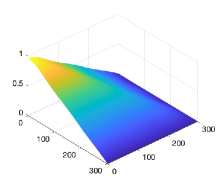
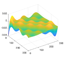
Figure 8: Fitting the uniform attachment graphon limit $\mathbf{M}(x,y)=1-\max(x,y)$ with $(x,y)\in[0,1]^{2}$ following Procedure 3. The left is its approximation based on the $5$ most significant eigen directions and the right is the approximation error. We first sample a matrix of size $300\times 300$ from the limit based on the uniform grid of $[0,1]^{2}$ for the uniform attachment graphon limit; then we compute the eigen decomposition of the matrix and proceed to identify the 5 most significant eigenvalues; afterwards, we approximate (or identify) the eigenvectors by sinusoidal fit (in fact, from the shape of the actual eigenvector, it is quite clear the associated graphon eigenfunctions are sinusoidal functions).

The procedure is suitable for any graphon. The size of the sampling matrices can be chosen according to the available computational resources and the error tolerance for approximations. For the procedure to approximate eigenfunctions based on Fourier functions and the approximation error, readers are referred to [45, Chapter 2] and [16].

The properties of graphon eigenfunctions can be inferred from the properties of the graphon, which may be used to identify suitable function classes to approximate eigenfunctions.

Proposition 11 (Differentiability)

If a graphon $\mathbf{M}\in\mathcal{W}_{c}$ is differentiable with respect to the nodal index in $[0,1]$ almost everywhere up to the $k$ order ($k\geq 1$), then the eigenfunctions of $\mathbf{M}$ associated with non-zero eigenvalues which are uniformly bounded away from zero are differential up to the $k$ order almost everywhere with respect to the nodal index in $[0,1]$.

Proof

Consider any normalized eigenvector $\mathbf{u}$ of $\mathbf{M}$. If there exists $L>0$ such that for all $\beta\in[0,1]$,

$$\left|\frac{d^{i}}{d\alpha^{i}}\mathbf{M}(\alpha,\beta)\right|\leq L,\quad\forall i\in\{1,...,k\},\text{for almost all}~{}\alpha\in[0,1],$$

then for almost all $\alpha\in[0,1]$,

$$\left|\frac{d^{i}}{d\alpha^{i}}\left([\mathbf{M}\mathbf{u}](\alpha)\right)\right| =\left|\frac{d^{i}}{d\alpha^{i}}\left(\int_{0}^{1}\mathbf{M}(\alpha,\beta)\mathbf{u}(\beta)d\beta\right)\right|$$

$$=\left|\left(\int_{0}^{1}\frac{d^{i}}{d\alpha^{i}}\mathbf{M}(\alpha,\beta)\mathbf{u}(\beta)d\beta\right)\right|$$

$$\leq L\left|\int_{0}^{1}\mathbf{u}(\beta)\right|d\beta\leq L\|\mathbf{u}\|_{2}=L.$$

Based on the definition of eigenfunction, for $\lambda\neq 0$, we know $\mathbf{u}(\alpha)=\frac{1}{\lambda}\frac{d^{i}}{d\alpha^{i}}\left([\mathbf{M}\mathbf{u}](\alpha)\right)$ for all $\alpha\in[0,1]$. That is the eigenvector is differentiable up to order $k$ almost everywhere.

Proposition 12 (Lipschitz Continuity)

Consider a graphon $\mathbf{M}\in\mathcal{W}_{c}$. If there exists $L>0$ such that

$$|\mathbf{M}(\alpha,\beta)-\mathbf{M}(\gamma,\eta)|<L(|\alpha-\gamma|+|\beta-\eta|),$$ (116)

then any eigenfunction of $\mathbf{M}$ associated with nonzero eigenvalues which are uniformly bounded away from zero is Lipschitz continuous.

Proof

Let $\mathbf{u}\in L^{2}[0,1]$ be any normalized eigenvector of $\mathbf{M}$, that is $\mathbf{M}\mathbf{u}=\lambda\mathbf{u}$ with $\lambda\in\mathds{R}$. Then

$$\big{|}[\mathbf{M}\mathbf{u}](\alpha)-[\mathbf{M}\mathbf{u}](\beta)\big{|}=\left|\int_{0}^{1}(\mathbf{M}(\alpha,\gamma)-\mathbf{M}(\beta,\gamma))\mathbf{u}(\gamma)d\gamma\right|$$

$$\leq\int_{0}^{1}\left|(\mathbf{M}(\alpha,\gamma)-\mathbf{M}(\beta,\gamma))\mathbf{u}(\gamma)\right|d\gamma$$

$$<L|\alpha-\beta|\int_{0}^{1}|\mathbf{u}(\gamma)|d\gamma\leq L|\alpha-\beta|\|\mathbf{u}\|_{2}=L|\alpha-\beta|.$$

That is $\mathbf{M}\mathbf{u}$ is Lipschitz continuous. For $\lambda\neq 0$ that is uniformly bounded away from zero, we know that $\mathbf{u}=\frac{1}{\lambda}\mathbf{M}\mathbf{u}$ is also Lipschitz continuous.

A function $f:\Omega\to\mathds{R}$ with $\Omega\subset\mathds{R}^{n}$ is called $\alpha$-Hölder continuous ($\alpha>0$) if there exists a constant $C>0$ such that

$$|f(x)-f(y)|\leq C\|x-y\|^{\alpha}.$$

When $\alpha=1$, $\alpha$-Hölder continuity is then equivalent to the Lipschitz continuity. A function is $\alpha$-Hölder with $\alpha>1$ is constant and $\alpha$-Hölder continuity implies uniform continuity. Applying this definition to graphons, we know that a graphon $\mathbf{M}\in\mathcal{W}_{c}$ is $\alpha$-Hölder continuous ($\alpha>0$) if there exist a constant $C>0$ for all $(x_{1},y_{1}),(x_{2},y_{2})\in[0,1]^{2}$ such that

$$|\mathbf{M}(x_{1},y_{1})-\mathbf{M}(x_{2},y_{2})|\leq C\big{(}\sqrt{|(x_{1}-x_{2})^{2}+(y_{1}-y_{2})^{2}|}\big{)}^{\alpha}.$$

Here we use the Euclidean norm for points $[0,1]^{2}\subset\mathds{R}^{2}$, but clearly it can be replaced by any equivalent norm.

Proposition 13 (Hölder Continuity)

If a graphon $\mathbf{M}\in\mathcal{W}_{c}$ is $\alpha$-Hölder continuous ($\alpha>0$), then its eigenfunctions associated with non-zero eigenvalues which are uniformly bounded away from zero are $\alpha$-Hölder continuous.

Proof

Let $\mathbf{u}\in L^{2}[0,1]$ be any normalized eigenvector of $\mathbf{M}$, that is $\mathbf{M}\mathbf{u}=\lambda\mathbf{u}$ with $\lambda\in\mathds{R}$. Then

$$\big{|}[\mathbf{M}\mathbf{u}](x)-[\mathbf{M}\mathbf{u}](y)\big{|}=\left|\int_{0}^{1}(\mathbf{M}(x,\gamma)-\mathbf{M}(y,\gamma))\mathbf{u}(\gamma)d\gamma\right|$$ (117)

$$\leq\int_{0}^{1}\left|(\mathbf{M}(x,\gamma)-\mathbf{M}(y,\gamma))\right||\mathbf{u}(\gamma)|d\gamma$$

$$<C|x-y|^{\alpha}\int_{0}^{1}|\mathbf{u}(\gamma)|d\gamma\leq C|x-y|^{\alpha}\|\mathbf{u}\|_{2}=C|x-y|^{\alpha}.$$

Since for $\lambda\neq 0$, $\mathbf{u}=\frac{1}{\lambda}\mathbf{M}\mathbf{u}$, we obtain

$$|\mathbf{u}(x)-\mathbf{u}(y)|\leq C\frac{1}{|\lambda|}|x-y|^{\alpha},\quad\forall x,y\in[0,1],$$

that is, $\mathbf{u}$ is $\alpha$-Hölder continuous.

Appendix E Idempotent Couplings

A matrix $X$ is idempotent if $X^{2}=X$. The eigenvalues of any idempotent matrix are either $0$ or $1$. Idempotent matrices are not necessarily symmetric.

Proposition 14 (Idempotent Couplings)

If the coupling $\bar{M}\triangleq\frac{1}{N}M$ is idempotent (that is $\bar{M}^{2}=\bar{M}$), $\eta=0$, and for every $q\in\{1,...,N\}$ there exists a unique solution pair $(\bar{s}_{q},\bar{z}_{q})$ to the following coupled forward-backward equations

$$- \dot{\bar{s}}_{q}(t)=A_{c}(t)^{\mathchoice{\raisebox{0.0pt}{$\displaystyle\intercal$}}{\raisebox{0.0pt}{$\textstyle\intercal$}}{\raisebox{0.0pt}{$\scriptstyle\intercal$}}{\raisebox{0.0pt}{$\scriptscriptstyle\intercal$}}}\bar{s}_{q}(t)-(QH-\Pi_{t}D)\bar{z}_{q}(t),$$ (118)

$$\dot{\bar{z}}_{q}(t)=(A_{c}(t)+D)\bar{z}_{q}(t)-BR^{-1}B^{\mathchoice{\raisebox{0.0pt}{$\displaystyle\intercal$}}{\raisebox{0.0pt}{$\textstyle\intercal$}}{\raisebox{0.0pt}{$\scriptstyle\intercal$}}{\raisebox{0.0pt}{$\scriptscriptstyle\intercal$}}}\bar{s}_{q}(t),$$ (119)

with boundary conditions $\bar{s}_{q}(T)=Q_{T}H\bar{z}_{q}(T)$ and $\bar{z}_{q}(0)=\frac{1}{N}\sum_{\ell=1}^{N}m_{q\ell}\bar{x}_{\ell}(0),$ where $t\in[0,T]$, $A_{c}(t)\triangleq(A-BR^{-1}B^{\mathchoice{\raisebox{0.0pt}{$\displaystyle\intercal$}}{\raisebox{0.0pt}{$\textstyle\intercal$}}{\raisebox{0.0pt}{$\scriptstyle\intercal$}}{\raisebox{0.0pt}{$\scriptscriptstyle\intercal$}}}\Pi_{t})$, and $\Pi_{(\cdot)}$ is the solution to the $n\times n$-dimensional matrix Riccati equation

$$-\dot{\Pi}_{t}=A^{\mathchoice{\raisebox{0.0pt}{$\displaystyle\intercal$}}{\raisebox{0.0pt}{$\textstyle\intercal$}}{\raisebox{0.0pt}{$\scriptstyle\intercal$}}{\raisebox{0.0pt}{$\scriptscriptstyle\intercal$}}}\Pi_{t}+\Pi_{t}A-\Pi_{t}BR^{-1}B^{\mathchoice{\raisebox{0.0pt}{$\displaystyle\intercal$}}{\raisebox{0.0pt}{$\textstyle\intercal$}}{\raisebox{0.0pt}{$\scriptstyle\intercal$}}{\raisebox{0.0pt}{$\scriptscriptstyle\intercal$}}}\Pi_{t}+Q,~{}\Pi_{T}=Q_{T},$$ (120)

then the game problem defined by (16) and (17) has a unique Nash equilibrium and the best response in the equilibrium is given as follows: for a generic agent $\alpha$ in cluster $\mathcal{C}_{q}$,

$$u_{\alpha}(t) =-R^{-1}B^{\mathchoice{\raisebox{0.0pt}{$\displaystyle\intercal$}}{\raisebox{0.0pt}{$\textstyle\intercal$}}{\raisebox{0.0pt}{$\scriptstyle\intercal$}}{\raisebox{0.0pt}{$\scriptscriptstyle\intercal$}}}(\Pi_{t}x_{\alpha}(t)+\bar{s}_{q}(t)),~{}\alpha\in\mathcal{C}_{q},~{}q\in\mathcal{V}_{c}.$$ (121)

Proof

Within an infinite nodal population, the individual effect on the nodal mean field is negligible. Hence each individual agent in cluster $\mathcal{C}_{q}$ is solving a LQG tracking problem to track a reference trajectory $\nu_{q}$. The best response for a generic agent $\alpha$ in cluster $\mathcal{C}_{q}$ is simply given by the optimal LQG tracking solution as

$$u_{\alpha}(t) =-R^{-1}B^{\mathchoice{\raisebox{0.0pt}{$\displaystyle\intercal$}}{\raisebox{0.0pt}{$\textstyle\intercal$}}{\raisebox{0.0pt}{$\scriptstyle\intercal$}}{\raisebox{0.0pt}{$\scriptscriptstyle\intercal$}}}(\Pi_{t}x_{\alpha}(t)+\bar{s}_{q}(t)),\qquad\alpha\in\mathcal{C}_{q}$$ (122)

where $\Pi$ is given by (21) and $\bar{s}_{q}$ is given by

$$-\dot{\bar{s}}_{q}(t) =\big{(}A-BR^{-1}B^{\mathchoice{\raisebox{0.0pt}{$\displaystyle\intercal$}}{\raisebox{0.0pt}{$\textstyle\intercal$}}{\raisebox{0.0pt}{$\scriptstyle\intercal$}}{\raisebox{0.0pt}{$\scriptscriptstyle\intercal$}}}\Pi_{t}\big{)}^{\mathchoice{\raisebox{0.0pt}{$\displaystyle\intercal$}}{\raisebox{0.0pt}{$\textstyle\intercal$}}{\raisebox{0.0pt}{$\scriptstyle\intercal$}}{\raisebox{0.0pt}{$\scriptscriptstyle\intercal$}}}{\bar{s}}_{q}(t)-Q\nu_{q}(t){+\Pi_{t}D\bar{z}_{q}}(t),$$ (123)

$$\bar{s}_{q}{(T)} =Q_{T}\nu_{q}(T),$$

and $\nu_{q}(t)\triangleq H\bar{z}_{q}(t)$. If all agents follow the best response in (121), then the evolution of the $\bar{z}$ process satisfy

$$\dot{\bar{z}}_{q}(t)= ~{}(A-BR^{-1}B^{\mathchoice{\raisebox{0.0pt}{$\displaystyle\intercal$}}{\raisebox{0.0pt}{$\textstyle\intercal$}}{\raisebox{0.0pt}{$\scriptstyle\intercal$}}{\raisebox{0.0pt}{$\scriptscriptstyle\intercal$}}}\Pi_{t})\bar{z}_{q}(t)+D\frac{1}{N}\sum_{\ell=1}^{N}m_{q\ell}\bar{z}_{\ell}(t)$$ (124)

$$\quad-BR^{-1}B^{\mathchoice{\raisebox{0.0pt}{$\displaystyle\intercal$}}{\raisebox{0.0pt}{$\textstyle\intercal$}}{\raisebox{0.0pt}{$\scriptstyle\intercal$}}{\raisebox{0.0pt}{$\scriptscriptstyle\intercal$}}}\frac{1}{N}\sum_{\ell=1}^{N}m_{q\ell}\bar{s}_{\ell}(t)$$

with initial condition $\bar{z}_{q}(0)=\frac{1}{N}\sum_{\ell=1}^{N}m_{q\ell}\bar{x}_{\ell}(0),\quad 1\leq q\leq N.$ Since $\frac{1}{N}M$ is idempotent and $\bar{z}(t)=\frac{1}{M}\bar{x}(t)$, we obtain $\frac{1}{N}M\bar{z}(t)=\bar{z}(t)$ and equivalently $D\frac{1}{N}\sum_{\ell=1}^{N}m_{q\ell}\bar{z}_{\ell}(t)=D\bar{z}_{q}(t).$ Furthermore, let us define $\bar{\bar{s}}(t)\triangleq\frac{1}{N}M\bar{s}(t)$. Then (124) becomes

$$\dot{\bar{z}}_{q}(t)= ~{}(A-BR^{-1}B^{\mathchoice{\raisebox{0.0pt}{$\displaystyle\intercal$}}{\raisebox{0.0pt}{$\textstyle\intercal$}}{\raisebox{0.0pt}{$\scriptstyle\intercal$}}{\raisebox{0.0pt}{$\scriptscriptstyle\intercal$}}}\Pi_{t})\bar{z}_{q}(t)+D\bar{z}_{q}(t)-BR^{-1}B^{\mathchoice{\raisebox{0.0pt}{$\displaystyle\intercal$}}{\raisebox{0.0pt}{$\textstyle\intercal$}}{\raisebox{0.0pt}{$\scriptstyle\intercal$}}{\raisebox{0.0pt}{$\scriptscriptstyle\intercal$}}}\bar{\bar{s}}_{q}(t)$$ (125)

$$\bar{z}_{q}(0)= ~{}\frac{1}{N}\sum_{\ell=1}^{N}m_{q\ell}\bar{x}_{\ell}(0),\quad 1\leq q\leq N.$$

Similarly, from $\nu_{q}\triangleq H\bar{z}_{q}$, we obtain that $\frac{1}{N}M\nu=\nu$.

Therefore, from (123), $\bar{\bar{s}}$ satisfies

$$-\dot{\bar{\bar{s}}}_{q}(t) =\big{(}A-BR^{-1}B^{\mathchoice{\raisebox{0.0pt}{$\displaystyle\intercal$}}{\raisebox{0.0pt}{$\textstyle\intercal$}}{\raisebox{0.0pt}{$\scriptstyle\intercal$}}{\raisebox{0.0pt}{$\scriptscriptstyle\intercal$}}}\Pi_{t}\big{)}^{\mathchoice{\raisebox{0.0pt}{$\displaystyle\intercal$}}{\raisebox{0.0pt}{$\textstyle\intercal$}}{\raisebox{0.0pt}{$\scriptstyle\intercal$}}{\raisebox{0.0pt}{$\scriptscriptstyle\intercal$}}}{\bar{\bar{s}}}_{q}(t)-Q\nu_{q}(t){+\Pi_{t}D\bar{z}_{q}}(t),$$ (126)

$$\bar{\bar{s}}_{q}{(T)} =Q_{T}H\bar{z}_{q}(T)$$

where $\nu_{q}(t)\triangleq H\bar{z}_{q}(t)$. This is exactly the same equation as (123) and hence this implies that $\bar{\bar{s}}=\bar{s}$. If there exists a unique solution pair $(\bar{z}_{q}(t),\bar{s}_{q}(t))_{q\in\mathcal{V}_{c},t\in[0,T]}$ to equations (123) and (124), then the best response strategy for each agent is uniquely determined by (122), (120), (123) and (124). The joint equations (123) and (124) can be equivalently represented by the two $n$-dimensional equations as (118) and (119).

Remark 7

Important features for LQG-GMFG problems with idempotent couplings are that the solution equations (118) and (119) are $n$-dimensional and independent of the network structure, and the only network couplings among different nodes in the solutions appear in the initial condition $\bar{z}(0)$. Mean field coupling can be considered a special case of idempotent couplings (with rank one).

References

• [1] S. Gao, P. E. Caines, and M. Huang, “LQG graphon mean field games: Graphon invariant subspaces,” Accepted by the 60th IEEE Conference on Decision and Control, 2021.
• [2] P. E. Caines and M. Huang, “Graphon mean field games and the GMFG equations,” in Proceedings of the 57th IEEE Conference on Decision and Control (CDC), December 2018, pp. 4129–4134.
• [3] ——, “Graphon mean field games and the GMFG equations: $\varepsilon$-Nash equilibria,” in Proceedings of the 58th IEEE Conference on Decision and Control (CDC), December 2019, pp. 286–292.
• [4] ——, “Graphon mean field games and the GMFG equations,” SIAM Journal on Control and Optimization (to appear), 2021, arXiv:2008.10216.
• [5] C. Borgs, J. T. Chayes, L. Lovász, V. T. Sós, and K. Vesztergombi, “Convergent sequences of dense graphs i: Subgraph frequencies, metric properties and testing,” Advances in Mathematics, vol. 219, no. 6, pp. 1801–1851, 2008.
• [6] ——, “Convergent sequences of dense graphs ii. multiway cuts and statistical physics,” Annals of Mathematics, vol. 176, no. 1, pp. 151–219, 2012.
• [7] L. Lovász, Large Networks and Graph Limits.   American Mathematical Soc., 2012, vol. 60.
• [8] G. S. Medvedev, “The nonlinear heat equation on dense graphs and graph limits,” SIAM Journal on Mathematical Analysis, vol. 46, no. 4, pp. 2743–2766, 2014.
• [9] ——, “The nonlinear heat equation on w-random graphs,” Archive for Rational Mechanics and Analysis, vol. 212, no. 3, pp. 781–803, 2014.
• [10] H. Chiba and G. S. Medvedev, “The mean field analysis of the Kuramoto model on graphs I. the mean field equation and transition point formulas,” Discrete and Continuous Dynamical Systems-Series A, vol. 39, no. 1, pp. 131–155, 2019.
• [11] E. Bayraktar, S. Chakraborty, and R. Wu, “Graphon mean field systems,” arXiv preprint arXiv:2003.13180, 2020.
• [12] M. Avella-Medina, F. Parise, M. T. Schaub, and S. Segarra, “Centrality measures for graphons: Accounting for uncertainty in networks,” IEEE Transactions on Network Science and Engineering, vol. 7, no. 1, pp. 520–537, 2018.
• [13] J. Petit, R. Lambiotte, and T. Carletti, “Random walks on dense graphs and graphons,” arXiv preprint arXiv:1909.11776, 2019.
• [14] L. Ruiz, L. F. Chamon, and A. Ribeiro, “The graphon Fourier transform,” arXiv preprint arXiv:1910.10195, 2019.
• [15] L. Ruiz, F. Gama, and A. Ribeiro, “Graph neural networks: Architectures, stability and transferability,” arXiv preprint arXiv:2008.01767, 2020.
• [16] S. Gao and P. E. Caines, “Spectral representations of graphons in very large network systems control,” in Proceedings of the 58th IEEE Conference on Decision and Control (CDC), Nice, France, December 2019, pp. 5068–5075.
• [17] R. Vizuete, P. Frasca, and F. Garin, “Graphon-based sensitivity analysis of sis epidemics,” IEEE Control Systems Letters, vol. 4, no. 3, pp. 542–547, 2020.
• [18] S. Gao and P. E. Caines, “The control of arbitrary size networks of linear systems via graphon limits: An initial investigation,” in Proceedings of the 56th IEEE Conference on Decision and Control (CDC), Melbourne, Australia, December 2017, pp. 1052–1057.
• [19] ——, “Graphon control of large-scale networks of linear systems,” IEEE Transactions on Automatic Control, vol. 65, no. 10, pp. 4090–4105, 2020.
• [20] ——, “Graphon linear quadratic regulation of large-scale networks of linear systems,” in Proceedings of the 57th IEEE Conference on Decision and Control (CDC), Miami Beach, FL, USA, December 2018, pp. 5892–5897.
• [21] ——, “Optimal and approximate solutions to linear quadratic regulation of a class of graphon dynamical systems,” in Proceedings of the 58th IEEE Conference on Decision and Control (CDC), Nice, France, December 2019, pp. 8359–8365.
• [22] ——, “Subspace decomposition for graphon LQR: Applications to VLSNs of harmonic oscillators,” IEEE Transactions on Control of Network Systems, vol. 8, no. 2, pp. 576–586, 2021, doi: 10.1109/TCNS.2021.3058923.
• [23] F. Parise and A. Ozdaglar, “Graphon games,” arXiv preprint arXiv:1802.00080, 2018.
• [24] R. Carmona, D. Cooney, C. Graves, and M. Lauriere, “Stochastic graphon games: I. the static case,” arXiv preprint arXiv:1911.10664, 2019.
• [25] S. Gao, R. Foguen Tchuendom, and P. E. Caines, “Linear quadratic graphon field games,” Communications in Information and Systems, vol. 21, no. 3, pp. 341–369, 2021.
• [26] D. Vasal, R. K. Mishra, and S. Vishwanath, “Sequential decomposition of graphon mean field games,” arXiv preprint arXiv:2001.05633, 2020.
• [27] M. O. Jackson and Y. Zenou, “Games on networks,” in Handbook of game theory with economic applications.   Elsevier, 2015, vol. 4, pp. 95–163.
• [28] Z. Han, D. Niyato, W. Saad, T. Başar, and A. Hjørungnes, Game theory in wireless and communication networks: theory, models, and applications.   Cambridge university press, 2012.
• [29] T. Başar and G. J. Olsder, Dynamic noncooperative game theory.   SIAM, 1998.
• [30] F. L. Lewis, H. Zhang, K. Hengster-Movric, and A. Das, Cooperative control of multi-agent systems: optimal and adaptive design approaches.   Springer Science & Business Media, 2013.
• [31] M. Huang, P. E. Caines, and R. P. Malhamé, “The NCE (mean field) principle with locality dependent cost interactions,” IEEE Transactions on Automatic Control, vol. 55, no. 12, pp. 2799–2805, 2010.
• [32] O. Guéant, “Existence and uniqueness result for mean field games with congestion effect on graphs,” Applied Mathematics & Optimization, vol. 72, no. 2, pp. 291–303, 2015.
• [33] F. Camilli and C. Marchi, “Stationary mean field games systems defined on networks,” SIAM Journal on Control and Optimization, vol. 54, no. 2, pp. 1085–1103, 2016.
• [34] F. Delarue, “Mean field games: A toy model on an Erdös-Renyi graph.” ESAIM. Proceedings and Surveys, vol. 60, 2017.
• [35] D. Lacker and A. Soret, “A case study on stochastic games on large graphs in mean field and sparse regimes,” arXiv preprint arXiv:2005.14102, 2020.
• [36] R. E. Showalter, Monotone operators in Banach space and nonlinear partial differential equations.   American Mathematical Soc., 1997, vol. 49.
• [37] A. Pazy, Semigroups of Linear Operators and Applications to Partial Differential Equations, ser. Applied Mathematical Sciences.   New York: Springer, 1983.
• [38] A. Bensoussan, G. Da Prato, M. C. Delfour, and S. Mitter, Representation and Control of Infinite Dimensional Systems, 2nd ed.   Springer Science & Business Media, 2007.
• [39] M. Huang, P. E. Caines, and R. P. Malhamé, “Social optima in mean field LQG control: centralized and decentralized strategies,” IEEE Transactions on Automatic Control, vol. 57, no. 7, pp. 1736–1751, 2012.
• [40] A. Bensoussan, K. Sung, S. C. P. Yam, and S.-P. Yung, “Linear-quadratic mean field games,” Journal of Optimization Theory and Applications, vol. 169, no. 2, pp. 496–529, 2016.
• [41] R. Salhab, R. P. Malhamé, and J. L. Ny, “Collective stochastic discrete choice problems: A Min-LQG dynamic game formulation,” IEEE Transactions on Automatic Control, vol. 65, no. 8, pp. 3302–3316, 2020.
• [42] S. Gao, P. E. Caines, and M. Huang, “LQG graphon mean field games,” arXiv preprint arXiv:2004.00679, 2021.
• [43] J. Munkres, Topology, 2nd ed.   Upper Saddle River, NJ : Prentice Hall, Inc, 2000.
• [44] M. Huang and M. Zhou, “Linear quadratic mean field games: Asymptotic solvability and relation to the fixed point approach,” IEEE Transactions on Automatic Control, vol. 65, no. 4, pp. 1397–1412, 2020.
• [45] S. Gao, “Graphon control theory for linear systems on complex networks and related topics,” Ph.D. dissertation, McGill University, 2019.
• [46] E. M. Airoldi, T. B. Costa, and S. H. Chan, “Stochastic blockmodel approximation of a graphon: Theory and consistent estimation,” in Advances in Neural Information Processing Systems, 2013, pp. 692–700.
• [47] S. Janson, “Graphons, cut norm and distance, couplings and rearrangements,” New York Journal of Mathematics, vol. 4, 2013.