Efficient hyperparameter tuning for kernel ridge regression with Bayesian optimization

Abstract

Machine learning methods usually depend on internal parameters – so called hyperparameters – that need to be optimized for best performance. Such optimization poses a burden on machine learning practitioners, requiring expert knowledge, intuition or computationally demanding brute-force parameter searches. We here address the need for more efficient, automated hyperparameter selection with Bayesian optimization. We apply this technique to the kernel ridge regression machine learning method for two different descriptors for the atomic structure of organic molecules, one of which introduces its own set of hyperparameters to the method. We identify optimal hyperparameter configurations and infer entire prediction error landscapes in hyperparameter space, that serve as visual guides for the hyperparameter dependence. We further demonstrate that for an increasing number of hyperparameters, Bayesian optimization becomes significantly more efficient in computational time than an exhaustive grid search – the current default standard hyperparameter search method – while delivering an equivalent or even better accuracy.

I Introduction

With the advent of datascience fourthparadigm ; Agrawala , data-driven research is becoming ever more popular in physics, chemistry and materials science Aykol/etal:2019 ; Himanen/Geurts/Foster/Rinke:2019 ; tms ; Rampi_review ; Zunger:2018 . Concomitantly, the importance of machine learning as a means to infer knowledge and predictions from the collected data is rising. Especially in molecular and materials science, machine learning has gained traction in the last years and now frequently complements other theoretical or experimental methods Rampi_review ; Zunger:2018 ; ma_deep_2015 ; shandiz_application_2016 ; gomez_design_2016 ; sendek_machine_2018 ; rlb2018 ; goldsmith_machine ; meyer_machine_2018 ; Gu/etal:2019 ; Schmidt/etal:2019 ; Jensen/etal:2020 ; Coley/etal:2020 .

The effective use of machine learning usually requires expert knowledge of the underlying model and the problem domain. A particular difficulty that is sometimes overlooked in current machine learning applications is the optimization of internal model parameters, so called hyperparameters. Non-expert data scientists often spend a long time exploring countless hyperparameter and model configurations for a given dataset before settling on the best one. However, the best settings for these hyperparameters change with different datasets and dataset sizes. The resulting machine learning model is frequently only applicable to one specific problem setting. New data requires hyperparameter re-optimization. Thus, expert use of machine learning is often a costly endeavor – both in terms of time and computational budget.

Optimal machine learning is achieved with the set of hyperparameters that optimize some score function $f$, such as mean absolute error (MAE), root mean squared error (RMSE), or coefficient of determination ($\mathrm{R}^{2}$). The score function reflects the quality of learning given the dataset composition and training set size, and is itself an unknown function of all $n$ hyperparameters $f$=$f(\{\bm{z}\})$. Hyperparameter tuning comprises a set of strategies to navigate the $n$-dimensional phase space of hyperparameters and pinpoint the parameter combination that brings about the best performance of the machine learning model.

The most commonly used form of automated hyperparameter tuning is grid search. Here the hyperparameter search space is discretised and an exhaustive search is launched across this grid. This brute-force technique is widely employed in machine learning libraries: the algorithm is easy to parallelise and is guaranteed to find the best solution. However, the number of possible parameter combinations to be explored grows exponentially with the number of hyperparameters $n$. Grid search becomes prohibitively expensive if more than 2 or 3 hyperparameters need to be optimized simultaneously.

One strategy to overcome this problem is to decompose the $n$-dimensional hyperparameter space into $n$ separate 1-dimensional spaces around each parameter, assuming no interdependence between them. The set of 1-dimensional grid searches can then be solved in turn, while keeping the values of other hyperparameters fixed. This approach is rarely pursued since hyperparameters are typically codependent: optimal solutions in each dimension depend on the fixed values and there is no guarantee that the correct overall solution can be found.

Hyperparameter tuning is a classic complex optimization problem, where the objective score function $f(\{\bm{z}\})$ has an unknown functional form, but can be evaluated at any point. An algorithm designed to address such tasks is Bayesian optimization srinivas_gaussian . It is widely applied in the machine learning community to tune hyperparameters of commonly used algorithms, such as random forest, deep neural network, deep forest or kernel methods wu_hyper_2019 ; Yogatama2014EfficientTL ; Perrone2019LearningSS ; olson_evaluation_2016 ; young_hyperspace_2018 , which are evaluated on a wide range of standard datasets from the UCI machine learning repository Dua:2019 . However, it is not yet common to apply Bayesian optimization to machine learning problems in the natural sciences, where high-dimensional hyperparameter spaces are frequently encountered.

In this study, we demonstrate the advantages of applying Bayesian optimization to a hyperparameter optimization problem in machine learning of computational chemistry. Our test case is a kernel ridge regression (KRR) machine learning model that maps molecular structures to their molecular orbital energies stuke_chemical_2019 . We represent the molecular structures with two different descriptors, the Coulomb matrix (rupp_fast_2012, ) and the many-body tensor representation huo_unified_2017 . The KRR method itself requires the optimization of two hyperparameters and one kernel choice. The Coulomb matrix is hyperparameter-free, but the many-body tensor representation adds up to 14 more hyperparameters to the model. Through pre-testing, we reduce this number to 2 hyperparameters that affect the model the most. The largest hyperparameter space we encounter in this approach is therefore 4 dimensional.

In previous work, we established the optimal kernels for the Coulomb matrix and the many-body tensor representation stuke_chemical_2019 . We set KRR hyperparameters by means of grid search for three different molecular datasets, after we had optimized the hyperparameters of the molecular descriptors manually beforehand stuke_chemical_2019 . Here, we take the more rigorous approach and combine the optimization of descriptor and model parameters into a hyperparameter search of up to four dimensions. Higher-dimensional searches are easily feasible with BOSS, but four dimensions already illustrate the efficiency of Bayesian optimization over grid search.

The objective of this manuscript is to evaluate the effectiveness and accuracy of BOSS against grid search in optimization problems with up to four dimensions. We show that already in 4 dimensions, BOSS outperforms grid search in terms of efficiency. In addition, we present score function landscapes generated across the hyperparameter phase space, and analyse them as a function of dataset size and composition. These landscapes provide insight into how the behavior of the machine learning model changes across a range of possible model configurations. Such insight helps machine learning practitioners to choose possible starting points for similar optimization problems.

The manuscript is organized as follows. Section II introduces the basic principle of machine learning with kernel ridge regression and illustrates how molecules are represented to the algorithm. The concept of hyperparameter tuning with grid search and Bayesian optimization is explained. In Section III, these two methods are applied to adjust the hyperparameters for our kernel ridge regression model which predicts molecular energies of three molecular datasets. We visualize and discuss our results. Conclusions and outlook are presented in the last section.

II methods

II.1 Machine learning model

We employ kernel ridge regression (KRR) to predict molecular orbital energies of three distinct datasets of organic molecules: the QM9 dataset of 134k small organic molecules (ramakrishnan_quantum_2014, ), the AA dataset of 44k conformers of proteinogenic amino acids (ropo_first_2016, ) and the OE dataset of 62 k organic molecules stuke_atomic_2020 . The three datasets have been described in detail in our previous KRR work and we refer the interested reader to Ref. stuke_chemical_2019, or the original references for each dataset for more information.

In KRR, a scalar target property, here the energy of the highest occupied molecular orbital (HOMO), is expressed as a linear combination of kernel functions $k(\bm{M},\bm{M^{\prime}})$

$$E^{\textnormal{pred}}(\bm{M})=\sum^{N}_{i=1}w_{i}k(\bm{M},\bm{M}_{i}).$$ (1)

$\bm{M}_{i}$ is the descriptor for molecule $i$ and the sum runs over all training molecules. $w_{i}$ are the regression weights that need to be learned.

In the scope of this work, we employ two kernel functions: the Gaussian kernel

$$k_{\textnormal{Gaussian}}(\bm{M},\bm{M}^{\prime})=e^{-\frac{||{\bm{M}-\bm{M}^{\prime}}||_{2}^{2}}{2\gamma^{2}}},$$ (2)

which is a function of the Euclidean distance between two molecules $\bm{M}$, $\bm{M}^{\prime}$, and the Laplacian kernel

$$k_{\textnormal{Laplacian}}(\bm{M},\bm{M}^{\prime})=e^{-\frac{||{\bm{M}-\bm{M}^{\prime}}||_{1}}{\gamma}},$$ (3)

which is based on the 1-norm to measure similarity between two molecules. In both cases, $\gamma$ is the kernel width that determines the resolution in molecular space.

The regression parameters $w_{i}$ are obtained from the minimization problem

$$\underset{w}{\textnormal{min}}\sum_{i=1}^{N}(E^{\textnormal{pred}}(\bm{M}_{i})-E^{\textnormal{ref}}_{i})^{2}+\alpha\bm{w}^{T}\mathbf{K}\bm{w},$$ (4)

where $E^{\textnormal{ref}}_{i}$ are the known reference HOMO energies in the dataset, $\mathbf{K}$ is the kernel matrix ($K_{i,j}:=k(\bm{M}_{i},\bm{M}_{j}$)) and $\bm{w}$ is the regression weight ($w_{i}$) vector. The scalar $\alpha$ controls the size of a regularization term and penalizes complex models with large regression weights over simpler models with small regression weights. Equation 4 has an analytic solution

$$\bm{w}=(\mathbf{K}+\alpha\mathbf{I})^{-1}\mathbf{E}^{\textnormal{ref}}$$ (5)

that determines $\bm{w}$.

We here explicitly distinguish between the regression weights $w_{i}$ and the hyperparameters of the machine learning model. The regression weights grow in number with increasing training data size and are given in closed mathematical form by eq. 5. Conversely, the hyperparameters are finite in number. In KRR, for example, the number of hyperparameters is fixed to two: $\alpha$ and $\gamma$. These two hyperparameters can assume any value within certain sensible ranges. Their optimal values have to be determined by an external hyperparameter tuning procedure. In addition, there are model-specific choices, which could be interpreted as special hyperparameters, that can only assume certain values. For KRR, this would be the choice of kernel.

II.2 Molecular representation

One important aspect in machine learning is the representation of the input data to the machine learning algorithm. Here we employ the Coulomb matrix (CM) (rupp_fast_2012, ) and the many-body tensor representation (MBTR) huo_unified_2017 . We use the DScribe package (dscribe, ) to generate both descriptors for the datasets in this work.

The entries of the CM are given by

$$C_{ij}=\begin{cases}0.5Z_{i}^{2.4}&\text{if $i=j$}\\ \frac{Z_{i}Z_{j}}{\lVert\mathbf{R_{i}}-\mathbf{R_{j}}\rVert}&\text{if $i\neq j$}\\ \end{cases}.$$ (6)

The CM encodes the nuclear charges $Z_{i}$ and corresponding Cartesian coordinates $R_{i}$ of all atoms $i$ in molecule $\bm{M}$. The off-diagonal elements represent a Coulomb repulsion between atom pairs and the diagonal elements have been fitted to the total energy of the corresponding atomic species in the gas phase. To enforce permutational invariance, the rows and columns of the CM are sorted with respect to their $\ell^{2}$-norm.

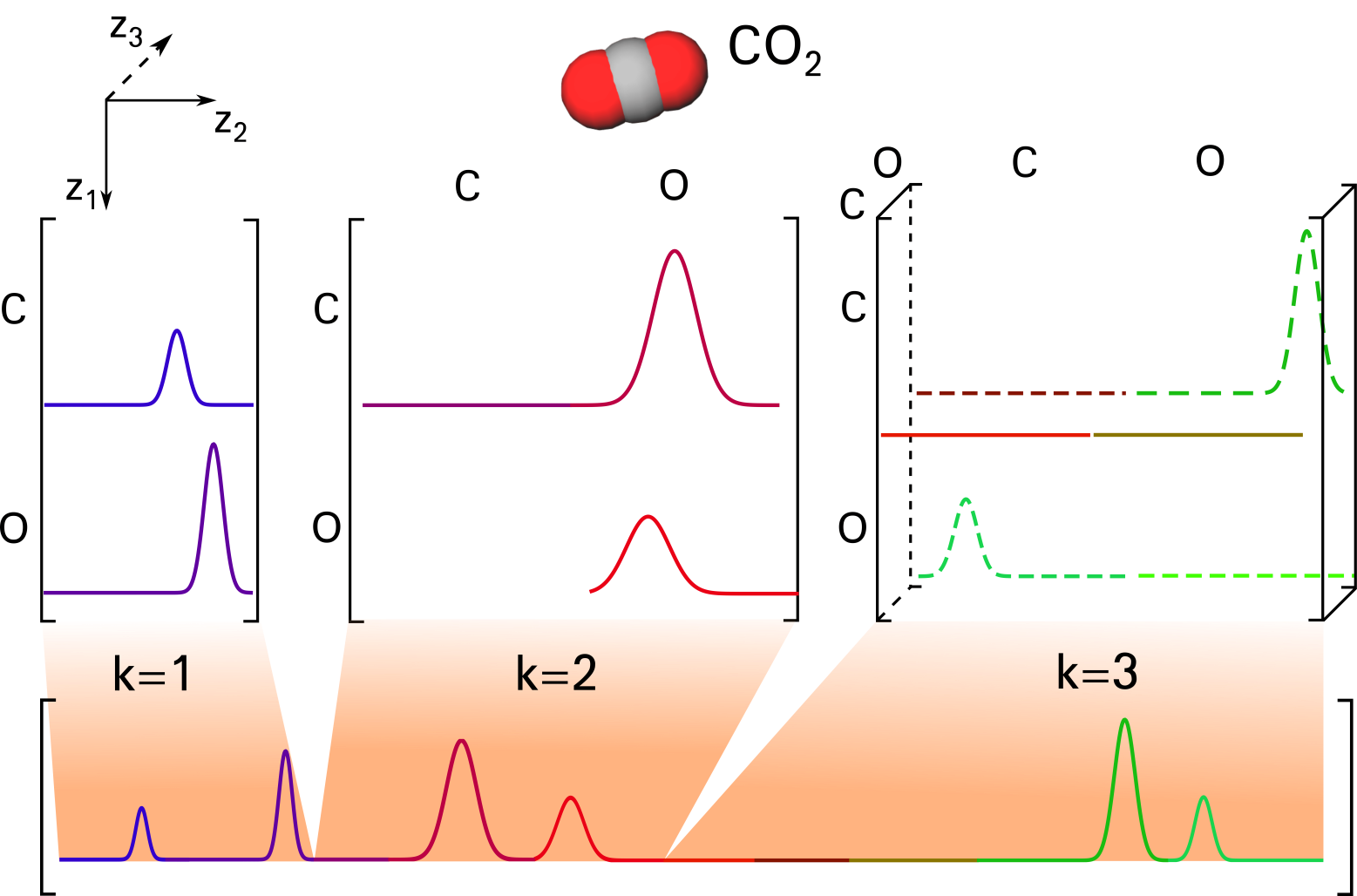
Figure 1: Illustration of the MBTR output for a CO₂ molecule, showing the distributions MBTR_k for $k$=1,2,3 with different combinations of chemical elements. The distributions of each $k$ term are arranged into a $k+1$ dimensional tensor.

The MBTR encodes molecular structures by decomposing them into a set of many-body terms (species, interatomic distances, bond angles, dihedral angles, etc.), as outlined for the example of a CO₂ molecule in Figure 1. Each many-body level is represented by a set of fixed sized vectors. The symbol $k$ enumerates the many-body level. We here include terms up to $k$=3. One-body terms ($k$=1) encode all atom types (species) present in the molecule. Two-body terms ($k$=2) encode pairwise inverse distances between any two atoms (bonded and non-bonded). Three-body terms ($k$=3) add angular distributions for any triple of atoms. A geometry function $g_{k}$ is used to transform each configuration of $k$ atoms into a single scalar value. These scalar values are then Gaussian broadened into continuous representations $\mathcal{D}_{k}$:

$$\mathcal{D}_{1}^{l}(x)=\frac{1}{\sigma_{1}\sqrt{2\pi}}e^{-\frac{(x-g_{1}(Z_{l}))^{2}}{2\sigma_{1}^{2}}}$$ (7)

$$\mathcal{D}_{2}^{l,m}(x)=\frac{1}{\sigma_{2}\sqrt{2\pi}}e^{-\frac{(x-g_{2}(\bm{R}_{l},\bm{R}_{m}))^{2}}{2\sigma_{2}^{2}}}$$ (8)

$$\mathcal{D}_{3}^{l,m,n}(x)=\frac{1}{\sigma_{3}\sqrt{2\pi}}e^{-\frac{(x-g_{3}(\bm{R}_{l},\bm{R}_{m}),\bm{R}_{n})^{2}}{2\sigma_{3}^{2}}}.$$ (9)

The $\sigma_{k}$’s are the feature widths for the different $k$-levels and $x$ runs over a predefined range $[x_{\textrm{min}}^{k},x_{\textrm{max}}^{k}]$ of possible values for the geometry functions $g_{k}$. For $k=1,2,3$, the geometry functions are given by $g_{1}(Z_{l})=Z_{l}$ (atomic number), $g_{2}(\bm{R}_{l},\bm{R}_{m})=|\bm{R}_{l}-\bm{R}_{m}|$ (distance) or $g_{2}(\bm{R}_{l},\bm{R}_{m})=\frac{1}{|\bm{R}_{l}-\bm{R}_{m}|}$ (inverse distance), and $g_{3}(\bm{R}_{l},\bm{R}_{m},\bm{R}_{n})=\textnormal{cos}(\angle(\bm{R}_{l}-\bm{R}_{m},\bm{R}_{n}-\bm{R}_{m}))$ (cosine of angle). For each possible combination of chemical elements present in the dataset, a weighted sum of distributions $\mathcal{D}_{k}$ is generated. For $k=1,2,3$, these final distributions are given by

$$\textnormal{MBTR}_{1}^{Z_{1}}(x)=\sum_{l}^{|Z_{1}|}w_{1}^{l}\mathcal{D}_{1}^{l}(x)$$ (10)

$$\textnormal{MBTR}_{2}^{Z_{1},Z_{2}}(x)=\sum_{l}^{|Z_{1}|}\sum_{m}^{|Z_{2}|}w_{2}^{l,m}\mathcal{D}_{2}^{l,m}(x)$$ (11)

$$\textnormal{MBTR}_{3}^{Z_{1},Z_{2},Z_{3}}(x)=\sum_{l}^{|Z_{1}|}\sum_{m}^{|Z_{2}|}\sum_{n}^{|Z_{3}|}w_{3}^{l,m,n}\mathcal{D}_{3}^{l,m,n}(x),$$ (12)

where the sums for $l$, $m$, and $n$ run over all atoms with atomic numbers $Z_{1}$, $Z_{2}$ and $Z_{3}$. $w_{k}$ are weighting functions that balance the relative importance of different $k$-terms and/or limit the range of inter-atomic interactions. For $k=1$, usually no weighting is used ($w_{1}^{l}=1$). For $k=2$ and $k=3$ the following exponential decay functions are implemented in DScribe

$$w_{2}^{l,m}=e^{-s_{k}|\bm{R}_{l}-\bm{R}_{m}|}$$ (13)

$$w_{3}^{l,m,n}=e^{-s_{k}(|\bm{R}_{l}-\bm{R}_{m}|+|\bm{R}_{m}-\bm{R}_{n}|+|\bm{R}_{l}-\bm{R}_{n}|)}$$ (14)

The parameter $s_{k}$ effectively tunes the cutoff distance. The functions MBTR${}_{k}(x)$ are then discretized with $n_{k}$ many points in the respective intervals $[x_{\textrm{min}}^{k},x_{\textrm{max}}^{k}]$.

II.3 Number and choice of hyperparameters

	Type	Number
KRR	feature width ($\gamma$)	1
	regularization ($\alpha$)	1
	kernel type	1
CM	none	0
MBTR	$k$-term feature widths ($\sigma_{k}$)	3
	weighting factors ($s_{k}$)	2
	discretization ($[x_{\textrm{min}}^{k},x_{\textrm{max}}^{k}]$, $n_{k}$)	9

Table 1: List of hyperparameter types and their total number in KRR, the CM and the MBTR.

In this section we review the hyperparameter types in our CM- or MBTR-based KRR models and motivate our choice for which hyperparameters to investigate in more detail. Table 1 gives an overview over all hyperparameters in this work. In total there would be 3 hyperparameters to optimize for CM-KRR and 17 for MBTR-KRR. Previous work has shown that some hyperparameters have little effect on the model. They can be preoptimized and set as defaults for the optimization of the remaining hyperparameters. We will explain this choice in more detail in the following.

The KRR method has 3 hyperparameters. $\gamma$ and $\alpha$ are continuous variables and need to be optimized. Conversely, the kernel choice can only assume certain finite values (0 and 1 in our case). We found in previous work stuke_chemical_2019 that the Laplacian kernel is more accurate for the CM representation and the Gaussian kernel for the MBTR. We therefore fix this choice also in this work and only optimize the 2 parameters $\gamma$ and $\alpha$.

The CM has no hyperparameters. Conversely, the MBTR introduces many. This indicates that the MBTR offers a more complex representation that could lead to faster learning for the same machine learning algorithm. This is indeed what we observed in our previous work comparing CM-KRR and MBTR-KRR stuke_chemical_2019 . However, the learning improvement comes at the price of a large number of hyperparameters, that need to be optimized to achieve a good model.

As Tab. 1 illustrates, MBTR introduces a total of 14 hyperparameters. In previous work stuke_chemical_2019 ; dscribe , we found that our KRR models were not sensitive to the grid discretization parameters. We therefore fix the grids to a range [0, 1] for $k=2$ and [-1, 1] for $k=3$, with 200 discretization points, and leave them unchanged for the rest of this study. We also found that the $k$=1 term does not improve the learning for the three datasets under investigation here stuke_chemical_2019 and therefore omit the $\sigma_{1}$ hyperparameter.

The molecules in our datasets are relatively small. We therefore do not need to limit the range of the MBTR and set $s_{2}=s_{3}=0$. This leaves us with 2 hyperparameters, the two feature widths $\sigma_{2}$ and $\sigma_{3}$. The minimum and maximum values of all hyperparameters in this study are listed in Table 2.

Hyperparameter	lower bound	upper bound
$\alpha$	1e-10	1
$\gamma$	1e-10	1e-3
$\sigma_{2}$	1e-6	1
$\sigma_{3}$	1e-6	1

Table 2: Hyperparameter search space for BOSS and grid search.

II.4 Hyperparameter tuning

Let $\bm{z}$ be a set of $n$ hyperparameters $\bm{z}={z_{1},z_{2},...,z_{n}}$, the boundaries of which define the hyperparameter search domain $\mathcal{Z}$, such that $\bm{z}\in\mathcal{Z}$. The score function $f({\bm{z}})\in\mathcal{Z}$ is a black-box function defined within the phase space $\mathcal{Z}$. The aim of hyperparameter optimization for a given machine learning model is to find the set of hyperparameters $\bm{\hat{z}}$ that provides the best model performance $\hat{y}$, as measured on a validation set:

$$\bm{\hat{z}}=\operatorname*{arg\,min}_{\mathbf{z}\in\mathcal{Z}}f(\bm{z}),\hskip 28.45274pt\hat{y}=f(\bm{\hat{z}})$$ (15)

The search for $\bm{\hat{z}}$ requires sampling the phase space $\mathcal{Z}$ through repeated $f(\bm{z})$ evaluations. Unfortunately, computing the objective function can be expensive. For each set of hyperparameters, it is necessary to train a model on the training data, make predictions on the validation data, and then calculate the validation metric. With an increasing number of hyperparameters, large datasets and complex models, this process quickly becomes intractable to do by hand. Therefore, automated hyperparameter tuning methods are indispensable tools for model building in machine learning.

In this study, we compare two approaches for hyperparameter tuning, grid search and Bayesian optimization. The former is guaranteed to find the optimal solution $\bm{\hat{z}}$, the latter is a statistical model with a high probability of finding $\bm{\hat{z}}$. Our score function $f(\bm{z})$ is the mean absolute error (MAE) on the prediction of HOMO energies, with units in eV.

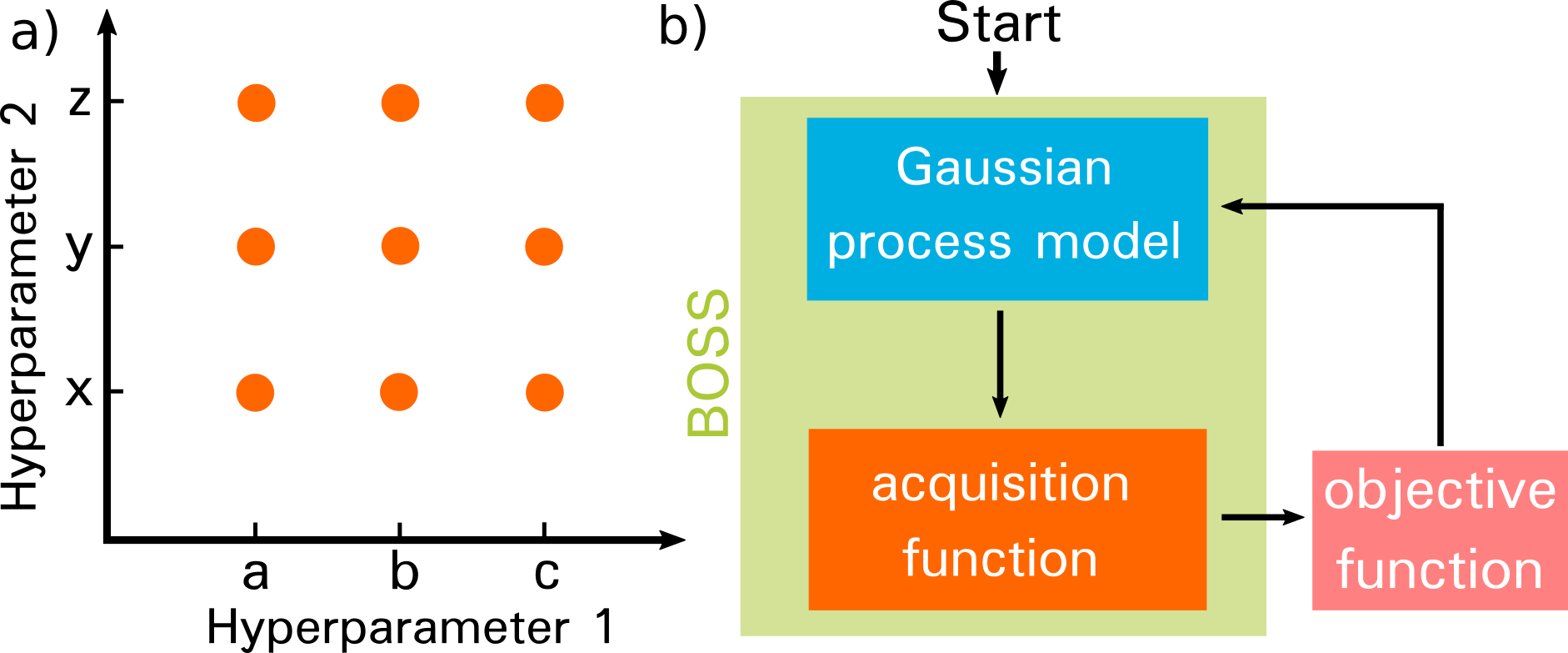
Figure 2: Working principles of hyperparameter tuning methods. a) In grid search, the hyperparameter space is mapped onto a grid, and the score function is evaluated for each combination of hyperparameter values. b) In Bayesian optimisation, a Gaussian process model is built to simulate the MAE landscape. The landscape is refined by sampling the score function across the hyperparameter space.

II.4.1 Grid Search

Grid search employs a grid of evenly spaced values for each hyperparameter $z$ to discretise the entire phase space $\mathcal{Z}$, as illustrated in Figure  2 a). The train-predict-evaluate cycle is then run automatically in a loop to evaluate the MAE for all hyperparameter configurations on the grid. Here, we rely on the scikit-learn implementation of KRR, but we eschew its native grid search function ’sklearn.model_selection.GridSearchCV’ in favour of own algorithms designed speficially for explicit evaluation of computational cost. Algorithms 1 and 2 demonstrate how the 2D and 4D grid searches were performed with different materials descriptors.

When the CM is used as molecular descriptor, we first compute a CM for each molecule in the dataset, as described in Algorithm 1. We shuffle the CMs and distribute them into five equally sized groups, along with their corresponding HOMO energies. We then set up a grid for the KRR hyperparameters $\alpha$ and $\gamma$ , with 11 values for each hyperparameter resulting in 121 grid points. Then, a 5-fold cross-validated KRR routine is performed for each possible combination of $\alpha$ and $\gamma$.

compute CM for all molecules ;

shuffle data and split into 5 equally sized groups ;

for $\alpha$ in $\{e^{j}|j=[-10,-9,...,0]\}$ do

       for $\gamma$ in $\{e^{j}|j=[-10,-9,...,0]\}$ do

             for group_i in [group₁, …, group₅] do

                   set group_i as validation set ;

                   set 4 remaining groups as training set ;

                   train KRR model with $\alpha$, $\gamma$ and Laplacian kernel on training set ;

                   validate model on validation set;

                  

             end for

            obtain 5 MAEs and compute average MAE $=\frac{1}{5}\sum_{i=1}^{5}\textnormal{MAE}_{i}$

       end for

      

end for

Algorithm 1 Grid search routine for 2D hyperparameter optimization with CM descriptor.

As usual in cross-validation, one of the split-off groups is defined as validation set and the remaining four groups combined serve as training set. A KRR model with the Laplacian kernel and the current combination of $\alpha$ and $\gamma$ is trained on the training set and prediction error MAE ($f(\alpha,\gamma)$) is computed on the validation set. For the next round of cross-validation, we define another group as validation set and the remaining four groups as training set to obtain a second MAE. In the same manner, more rounds of cross-validation are performed, until each of the 5 groups has been used as validation set once and as training set 4 times, resulting in 5 MAEs. The average of these serves as an MAE measure of how well the current combination of KRR hyperparameters performs for that grid point. Once we obtain an average MAE for each combination of $\alpha$ and $\gamma$ on the grid, we can pick the combination that results in the lowest MAE.

For the MBTR, we investigate 2D and 4D hyperparameter optimizations. The 2D case proceeds analogously to the CM KRR hyperparameter search, after we pick values for $\sigma_{2}$ and $\sigma_{3}$, and hold them fixed. The algorithm for the 4D case is depicted in Fig. 2. We loop over $\sigma_{2}$ and $\sigma_{3}$ on a logarithmic grid of six points each each and build the MBTR for the dataset for those values. Like the CM, this MBTR is then split into 5 subsets for cross validation. We then enter the $\alpha$ and $\gamma$ optimization as we do in the 2D grid search.

for $\sigma_{2}$ in $\{e^{j}|j=[-6,-5,...,0]\}$ do

      

      for $\sigma_{3}$ in $\{e^{j}|j=[-6,-5,...,0]\}$ do

            

            compute MBTR for all molecules;

             shuffle data and split into 5 equally sized groups ;

            

            for $\alpha$ in $\{e^{j}|j=[-10,-9,...,0]\}$ do

                   for $\gamma$ in$\{e^{j}|j=[-10,-9,...,0]\}$ do

                         for group_i in [group₁, …, group₅] do

                               set group_i as validation set ;

                               set 4 remaining groups as training set ;

                               train KRR model with $\alpha$, $\gamma$ and Gaussian kernel on training set ;

                               validate model on validation set;

                              

                         end for

                        obtain 5 MAEs and compute average MAE $=\frac{1}{5}\sum_{i=1}^{5}\textnormal{MAE}_{i}$

                   end for

                  

             end for

            

       end for

      

end for

Algorithm 2 Grid search routine for 4D hyperparameter optimization with MBTR descriptor.

II.4.2 Bayesian Optimization

With Bayesian optimization, we build a surrogate model for the MAE across the search domain, then iteratively refine it until convergence srinivas_gaussian ; rasmussen_gaussian ; gutmann_bayesian . Once the MAE surrogate landscape is known, it can be minimized efficiently to find the optimal choice of hyperparameters at its global minimum location. In this work, we rely on the Bayesian Optimization Structure Search (BOSS) package Todorovic/etal:2019 for simple and robust Bayesian optimization in physics, chemistry and materials science.

The Bayesian optimization algorithm, illustrated in Figure 2b), features a two-step procedure of Gaussian process regression (GPR), followed by an acqusition function. In the GPR, the MAE surrogate model is computed as the posterior mean of a Gaussian process (GP), given MAE data. This step produces an effective landscape of the MAE in hyperparameter space, which can be viewed and analysed. While the posterior mean is the statistically most likely fit to MAE data, the computed posterior variance (uncertainty) indicates which regions of the hyperparameter space are less well known. Both the mean and variance are then used to compute the eLCB acqusition function. The global minimum of the acqusition function points to the combination of hyperparameters in phase space to be tested next. Once this point is evaluated, the resulting MAE is added to the dataset and the cycle repeats. With each additional datapoint, the MAE surrogate model is improved. The method features variance and lengthscale hyperparameters encoded in the radial basis set (RBF) kernel of the Gaussian process, but these are autonomously refined along with the GPR model.

In this active learning technique, the data is collected at the same time as the model training is perfomed. The acquisition strategy combines data exploitation (searching near known minima) and exploration (searching previously unvisited regions of phase space) to quickly identify important regions of hyperparameter phase space where MAE is low. This allows us to identify the optimal combination of hyperparameters with relatively few MAE evaluations.

BOSS requires only the range of hyperparameters as input, so it can define the phase space domain before it launches a fully automated $n$-dimensional search for the best combination of hyperparameters. Acquisitions are made according to Algorithms 3 and 4, which serve as the evaluation function. For each new acquisition, the molecular descriptor (either CM or MBTR) is computed and KRR with 5-fold cross validation is performed. The average MAE is returned to BOSS to refine the MAE surrogate model and to perform the next acquisition.

Once the $n$-dimensional MAE surrogate models are converged, we can evaluate model accuracy qualitatively and model predictions quantitatively. Model predictions are summarised by the location of the global minimum in hyperparameter space $\bm{\hat{z}}$, and its value in the surrogate model $\mu(\bm{\hat{z}})$. Although $\mu(z)$ values should be close to the true $f(z)$ score function values, we additionally evaluate $f(\bm{\hat{z}})$ to validate the match throughout the convergence cycle. This way we can determine that the model does converge, and that it coverges to the true function $f(z)$.

define boundaries for $\alpha$ and $\gamma$: $\alpha\in\{e^{j}|j=[-10,0]\}$, $\gamma\in\{e^{j}|j=[-10,0]\}$ ;

define number of iterations: n${}_{\textnormal{it}}$=150 ;

Acquisition function suggests new set of $\alpha$, $\gamma$ ;

compute CM for all molecules;

shuffle data and split into 5 equally sized groups ;

for group_i in [group₁, …, group₅] do

       set group_i as validation set ;

       set 4 remaining groups as training set ;

       train KRR model with $\alpha$, $\gamma$ and Laplacian kernel on training set ;

       validate model on validation set;

      

end for

obtain 5 MAEs and compute average MAE $=\frac{1}{5}\sum_{i=1}^{5}\textnormal{MAE}_{i}$ ;

return average MAE to GP model

Algorithm 3 2D hyperparameter optimization with CM descriptor: BOSS routine for objective function evaluation.

define boundaries for $\alpha$, $\gamma$, $\sigma_{2}$ and $\sigma_{3}$: $\alpha\in\{e^{j}|j=[-10,0]\}$, $\gamma\in\{e^{j}|j=[-10,0]\}$, $\sigma 2\in\{e^{j}|j=[-6,0]\}$, $\sigma_{3}\in\{e^{j}|j=[-6,0]\}$ ;

define number of iterations: n${}_{\textnormal{it}}$=300 ;

Acquisition function suggests new set of $\alpha$, $\gamma$, $\sigma_{2}$, $\sigma_{3}$ ;

compute MBTR for all molecules;

shuffle data and split into 5 equally sized groups ;

for group_i in [group₁, …, group₅] do

       set group_i as validation set ;

       set 4 remaining groups as training set ;

       train KRR model with $\alpha$, $\gamma$ and Gaussian kernel on training set ;

       validate model on validation set;

      

end for

obtain 5 MAEs and compute average MAE $=\frac{1}{5}\sum_{i=1}^{5}\textnormal{MAE}_{i}$;

return average MAE to GP model

Algorithm 4 4D hyperparameter optimization with MBTR descriptor: BOSS routine for objective function evaluation.

III Results and Discussion

In this section, we examine the performance of both grid search and BOSS in tuning the hyperparameters of KRR-based machine learning models for predicting molecular HOMO energies based on molecular structures. An important objective is to establish whether BOSS is capable of finding similar hyperparameter solutions as the grid search algorithm, which is guaranteed to succeed. BOSS solutions of $\bm{\hat{z}}$, $f(\bm{\hat{z}})$ and $\mu(\bm{\hat{z}})$ are presented in Table 5 alongside equivalent results from the grid search.

In this study we consider the case of CM and MBTR descriptors, which changes the dimensionality and complexity of the search. Concurrently, we analyze the effect of dataset type and training set size on the hyperparameter tuning procedure and optimal solutions. Finally, we compare timings of grid search and BOSS to estimate which approach is more efficient in each of the above described settings.

III.1 KRR-CM hyperparameter tuning

The CM materials descriptor has no parameters and the KRR kernel choice is clear. The MAE is thus a 2-dimensional function of KRR hyperparameters: regularization strength $\alpha$ and kernel width $\gamma$. Figure 3 shows the 2-dimensional landscapes of MAE of a CM-KRR model for the QM9 dataset and a training set size of 2k. Panel a) depicts the grid search and panel b) the BOSS results, with logarithmic axes for clarity. All BOSS searches in this and subsquent sections are converged with respect to the number of acquisitions. The detailed convergence analysis will be presented in Section III.4.

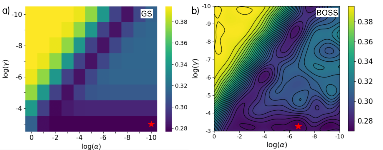
Figure 3: MAE landscapes from the 2D optimization problem with the CM as molecular descriptor. a) Grid search MAE as a function of hyperparameters $\alpha$ and $\gamma$, evaluated on a logarithmic grid. b) BOSS model prediction $\mu(z)$ of the MAE as a function of log($\alpha$) and log($\gamma$). Both grid search and BOSS were applied to a subset of 2k molecules taken from the QM9 dataset. Optimal hyperparameters are shown as red stars.

It is clear that BOSS and grid search produce qualitatively similar MAE landscapes. The grid search landscape is naturally "pixelated", because it only has a 10$\times$10 resolution in Fig. 3. Conversely, BOSS is not constrained to a grid and the Gaussian process in BOSS interpolates the MAE between the BOSS acquisitions.

Visualizing the MAE landscape tells us that the optimal parameter region has a complex and at first sight non-intuitive shape. The lowest MAE values in both methods lie on the diagonal of the hyperparameter landscape and along a horizontal line at the bottom of the landscape (for which $\gamma$ is $\sim$10^-3). Thus, the optimal parameter space has two parts: a co-dependent part, in which the choice of $\alpha$ and $\gamma$ is equally important for the KRR accuracy and a quasi one dimensional part, in which only the choice of $\gamma$ matters and $\alpha$ can assume any value. We will return to the analysis of this hyperparameter behavior in Section III.3.

Grid search and BOSS locate almost identical MAE minima: 0.277 eV for grid search and 0.270 eV for BOSS. The optimal hyperparameter solution $\bm{\hat{z}}$ found by BOSS and grid search are found in the same hyperparameter region of low log($\alpha$) values and high log($\gamma$) values. We conclude that BOSS is capable of reproducing grid search solutions to 1% accuracy in this case. Since BOSS and grid search produce qualitatively and quantitatively similar results, we will only consider BOSS MAE landscapes in the remaining discussion.

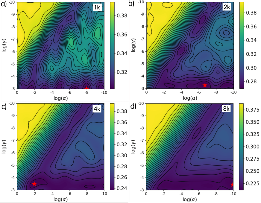
Figure 4: BOSS KRR-CM hyperparameter landscapes for increasing dataset sizes of the QM9 dataset. The figure style is the same as in Fig. 3.

Figure 4 illustrates BOSS MAE landscapes for increasing training set sizes of 1k, 2k, 4k and 8k molecules taken from the QM9 dataset. Tables 4 and 5 summarize the optimal hyperparameter search. We find that the MAE landscapes become more homogeneous with increasing dataset size and that the optimal MAE is decreasing (as expected). The optimal solution of hyperparameters $\bm{\hat{z}}$ vary somewhat, but are always found within the horizontal region at the large $\gamma$ values. The slight variation is an indication of the flat MAE landscapes in the aforementioned triangular solution space, on which many hyperparameter combinations yield low MAE values.

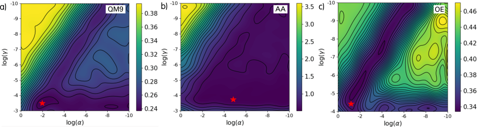
Figure 5: MAE landscapes of 2D BOSS hyperparameter optimization with CM as molecular descriptor. Shown is the predicted MAE $\mu(x)$ as a function of hyperparameters $\alpha$ and $\gamma$, evaluated on a logarithmic grid for three different datasets a) QM9, b) AA and c) OE. From each dataset, a subset of 4k molecules was used. Optimal hyperparameters are shown as red stars.

Next, we compare the hyperparameter landscapes across the three different molecular datasets QM9, AA and OE, as shown in Fig. 5. The model was trained on a subset of 4k molecules for each dataset. The dependence of MAE on the two KRR hyperparameters $\alpha$ and $\gamma$ is the same for all three datasets, with the the triangular region of optimal hyperparameters and flat MAE minima. However, the detailed dependence varies qualitatively with the dataset. For AA, the triangle is filled and we find a wide range of optimal hyperparameters in the landscape. This indicates that the KRR model is not overly sensitive to $\alpha$ and $\gamma$ for KRR-CM learning of the AA dataset. Conversely, for OE, the diagonal is more pronounced than the large $\gamma$ solution that dominates for QM9. The horizontal line of optimal hyperparameters has not yet developed for this training set size, indicating that broad feature widths $\gamma$ only lead to optimal learning when the regularization $\alpha$ is large. The optimal combination $\bm{\hat{z}}$ of hyperparameters differs across the three datasets (see Tables 4 -7 for optimal solutions $\bm{\hat{z}}$ and corresponding MAEs $f(\bm{\hat{z}})$ and $\mu(\bm{\hat{z}})$). Also the optimal MAE values vary considerably across the three datasets. This in accordance with our previous work, which revealed that the predictive power of KRR inherently depends on the complexity of the underlying dataset stuke_chemical_2019 .

III.2 KRR-MBTR 4D hyperparameter tuning

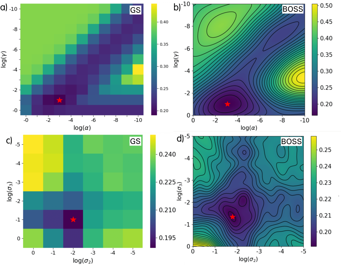
Figure 6: MAE landscapes from the 4D hyperparameter optimization problem with the MBTR descriptor. Panels a) and b) show 2D slices through the logarithmic ($\alpha$, $\gamma$) plane, while panels c) and d) show 2D slices through the logarithmic ($\sigma_{2}$, $\sigma_{3}$) plane. In a) and c), the grid search MAE and in b) and d), the BOSS MAE surrogate model $\mu(x)$ are presented. Both grid search and BOSS were applied to a subset of 2k molecules taken from the QM9 dataset. Optimal hyperparameters are shown as red stars.

We now consider the results of the 4D optimization problem, where the MBTR is used as molecular descriptor. BOSS builds a 4-dimensional surrogate model MAE($\alpha$,$\gamma$,$\sigma_{2}$, $\sigma_{3}$), which we compare to the reference 4-dimensional MAE landscape produced by grid search. Both 4D landscapes can be analyzed by considering 2-dimensional cross-sections. In Figure 6, we compare the BOSS surrogate model to the grid search result.

Figure 6 a) and b) illustrate the (log($\alpha$), log($\gamma$)) cross-section of the four dimensional MAE landscapes, extracted at the global minimum $\bm{\hat{z}}$ with optimal $\sigma_{2}$, $\sigma_{3}$ values. Similar to the MAE landscapes of the 2D optimization problem, the optimal values lie on a diagonal and on a horizontal line at the bottom of the map. A notable difference to the previously discussed 2D case are the lower overall prediction errors. This is in line with our previous finding stuke_chemical_2019 that the MBTR encodes the atomic structure of a molecule better than the CM.

In Figure 6 c) and d), the 4D MAE landscapes are cut through the (log($\sigma_{2}$), log($\sigma_{3}$)) plane, while $\alpha$ and $\gamma$ are held constant at their optimal values. Here, the optimal MAEs are found only within a small region. In contrast to the KRR hyperparameters, the MAE is barely sensitive to $\sigma_{2}$ and $\sigma_{3}$, varying only by two decimals throughout the map (about 10% of the value). All combinations of $\sigma_{2}$ and $\sigma_{3}$ are reasonably good choices for learning in this case.

As in the two dimensional CM case, BOSS and grid search reveal qualitatively consistent hyperparameter landscapes and optimal solutions $\bm{\hat{z}}$, $f(\bm{\hat{z}})$ and $\mu(\bm{\hat{z}})$ (see Table 5). Therefore, we will only discuss MAE landscapes produced by BOSS in the following.

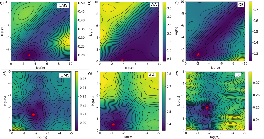
Figure 7: 2D-MAE landscapes from 4D BOSS hyperparameter optimization with MBTR as molecular descriptor. Shown is the predicted MAE $\mu(x)$ as a function of hyperparameters $\alpha$ and $\gamma$, evaluated on a logarithmic grid for three different datasets a) QM9, b) AA and c) OE. From each dataset, a subset of 2k molecules was used. Optimal hyperparameters are shown as red stars.

In Figure 7, we present BOSS MAE landscapes for the three different molecular datasets, where a subset of 2k molecules of each dataset was used for KRR. The comparison of the three MAE landscapes reveals that the QM9 dataset of small organic molecules is easiest to learn among all three datasets, since the MAE values are lowest. This is in accordance with the previous case of KRR-CM. We observe the highest MAEs for the AA dataset, which is most difficult to learn due to the higher chemical complexity of the molecules.

Panels a) - c) show MAE landscapes in logarithmic ($\alpha$ $\gamma$) planes and reveal the familiar diagonal pattern containing the lowest MAE. Compared to the 2D case with the CM descriptor, the landscapes are more homogeneous and the location $\bm{\hat{z}}$ of optimal hyperparameters lies within the same region for all three datasets. The choice of $\alpha$ and $\gamma$ seems to be independent of the dataset. Panels d) - f) show MAE landscapes in logarithmic ($\sigma_{2}$, $\sigma_{3}$) plane. All three datasets feature a cross-like shape of low MAE values. For QM9 and OE, the optimal MAE roughly lies on the crossover point. For these two datsets, the $\sigma_{2}$ and $\sigma_{3}$ values do not have a significant influence on the MAE range. For the AA dataset, in constrast, the choice of $\sigma_{2}$ and $\sigma_{3}$ dramatically affects the quality of learning and should be set correctly.

III.3 Interpretation of MAE landscapes

Figure 8: Schematic depiction of the observed optimal hyperparameter regions for two different hyperparameter spaces. a) Typical landscape in ($\alpha,\gamma$)-plane. b) Typical landscape in ($\sigma_{2},\sigma_{3}$)-plane.

We now discuss the distinctively different optimal regions of different hyperparameter classes. Figure 8 schematically depicts the shapes of these optimal hyper parameter regions for the KRR parameters ($\alpha$-$\gamma$ plane in panel a)) and the MBTR feature widths ($\sigma_{2}$-$\sigma_{3}$ plane in panel b)).

To understand the triangular shape in panel a), we have to recall the two kernels 2 and 3 and the KRR regularization equation eq. 4. For large feature widths $\gamma$, the abstract molecular space in which we measure distances between molecules $\boldmath{M}$ and $\boldmath{M^{\prime}}$, is filled with broad Laplacians or Gaussians. The kernel expansion in eq. 4 then picks up a contribution from almost any molecular pair $\boldmath{M}$ and $\boldmath{M^{\prime}}$. This means that the expansion coefficients have to be small. However, if the expansion coefficients are small, the regularization term is small and the size of the regularization strength $\alpha$ does not matter. This explains the horizontal line at the bottom of the triangle.

For smaller values of the feature width $\gamma$, the Laplacians or Gaussians in molecular space become narrower, until, in the limit of an infinitely small $\gamma$, we obtain delta functions. The narrower the expansion functions are in molecular space, the larger the expansion coefficients need to be to give finite target properties. When the expansion coefficients increase in size, however, the regularization parameter needs to reduce to keep the size of the penalty term low. $\gamma$ and $\alpha$ become co-dependent, which explains the diagonal line in the triangle.

For the MBTR hyperparameters, the situation is qualitatively different. Although $\sigma_{2}$ and $\sigma_{3}$ are also associated with feature widths, they control the broadening of features in the structural representation of molecular bond distances and angles. For large broadenings (i.e. large $\sigma_{2}$ and $\sigma_{3}$), peaks associated with individual features in the MBTR might merge and the MBTR looses resolution. For very small broadenings (i.e. very small $\sigma_{2}$ and $\sigma_{3}$) features are represented by very narrow peaks, which may not be captured by the MBTR grids. The MBTR again looses resolution. The hyperparameter sweet spot therefore lies in a roughly circular region of moderate $\sigma_{2}$ and $\sigma_{3}$ values. For our molecules and our datasets, the optimal $\sigma_{2}$ and $\sigma_{3}$ values are between 10^-1 and 10^-2, so closer to the bottom left corner of the hyperparameter landscape.

This section demonstrates that visualizing the hyperparameter landscapes greatly faciliates our understanding of the hyperparameter behavior in KRR and in machine learning in general. The BOSS methods provides an efficient way of generating easily readable landscapes that enable a deeper analysis of machine learning models.

III.4 Convergence, scaling and computational cost

III.4.1 Convergence

Figure 9 illustrates the convergence of BOSS as a function of iterations, using the CM and the MBTR as molecular descriptor, for different training set sizes. Here, we consider the global minimum location $\bm{\hat{z}}$ in the landscape as the surrogate model improves, compute its true MAE value $f(\bm{\hat{z}})$ and track the lowest value observed. In the limit of the predefined maximum number of iterations (100 for 2D and 300 for 4D) the model no longer changes, so we adopt the final MAEs $f(\bm{\hat{z}})$ as zero reference. In the final step, we subtract the reference from the sequence of lowest MAE values observed to obtain the bare convergence $\Delta f(\bm{\hat{z}})$ of the MAE with BOSS iteration steps.

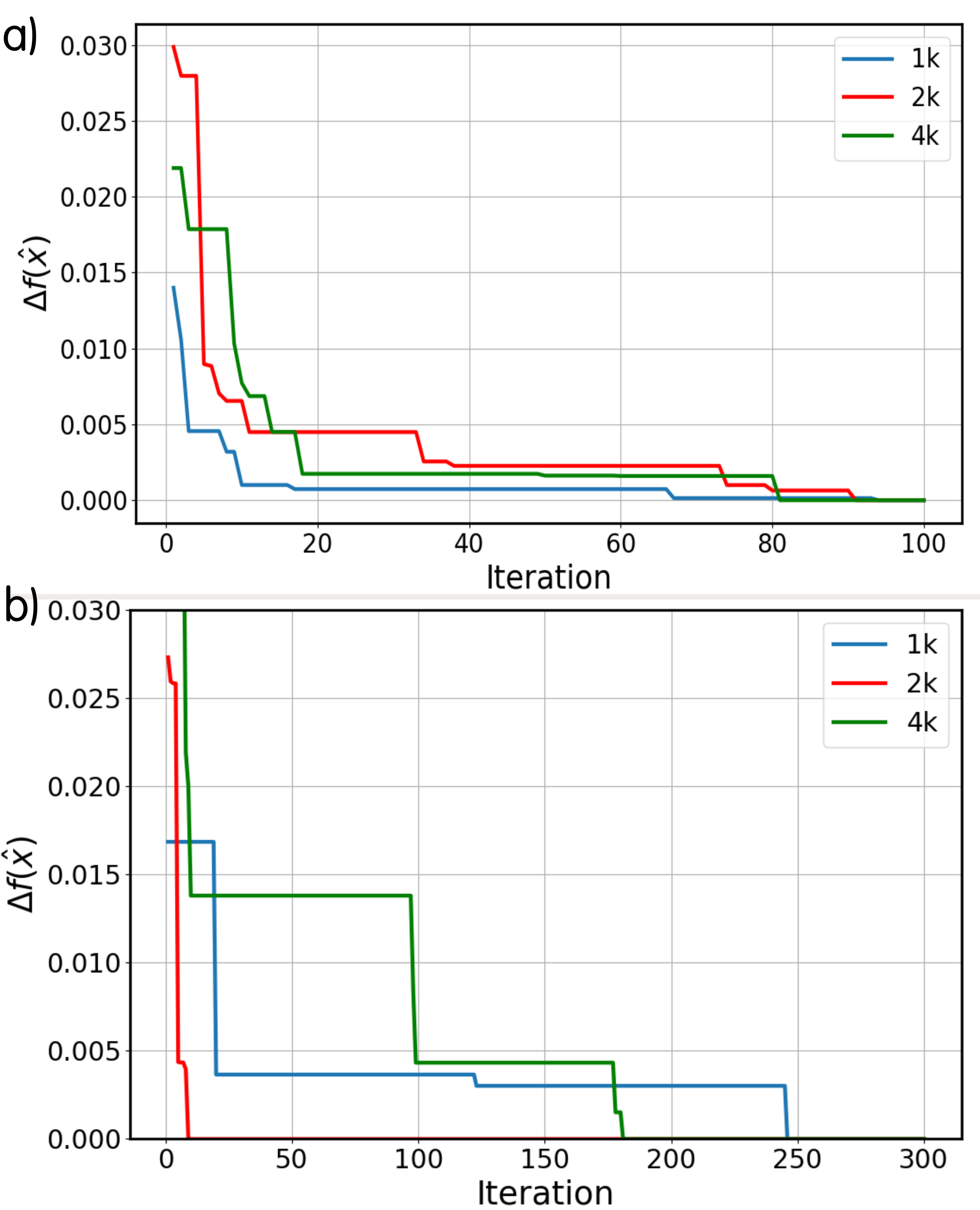
Figure 9: BOSS convergence as a function of iterations, performed on QM9 for three different training set sizes. Panel a) shows a 2D search with the CM and panel b) a 4D search with the MBTR as molecular descriptor. The convergence criterium $\Delta f(\hat{x})$ describes the difference between the currently lowest $f(\hat{x})$ and the lowest $f(\hat{x})$ after the maximum number of iterations.

Figure 9 shows that $\Delta f(\bm{\hat{z}})$ drops quickly with BOSS iterations. Since the best MAE resolution we achieved with grid search was 0.02eV, we define the BOSS convergence criteria as $\Delta f(\bm{\hat{z}})$)$\leq 10^{-2}$. We find that in the 2D case (KRR-CM in Fig. 9a)), the BOSS solution is already converged in fewer than 20 iterations, regardless of training set size. In the 4D hyperparameter search (KRR-MBTR in Fig. 9b)), BOSS reaches convergence in less than 50 iterations with underlying datasets of sizes 1k and 2k. For a dataset size of 4k, it takes almost 100 iterations to reach convergence. Some variation in convergence behaviour is expected, and averages from repeated runs would provide better averaged results in future work. Nonetheless, the best hyperparameter solutions were clearly found within 100 iterations in all scenarios.

III.4.2 Formal computational scaling

Formally, the computational time of a KRR run for a fixed training set size can be estimated as follows

$$t_{\textnormal{total}}=n_{\textnormal{desc}}\cdot\widetilde{t}_{\textnormal{desc}}+n_{\textnormal{KRR}}\cdot\widetilde{t}_{\textnormal{KRR}}+t_{\textnormal{process}}.$$

$\widetilde{t}_{\textnormal{desc}}$ is the average time to build the molecular descriptor for all molecules and $n_{\textnormal{desc}}$ is the number of times the descriptor has to be generated. $\widetilde{t}_{\textnormal{KRR}}$ is the average time to perform the 5-fold cross-validated KRR step to determine the regression coefficients $\boldmath{w}$ and $n_{\textnormal{KRR}}$ the number of times this has to be done. Finally, $\widetilde{t}_{\textnormal{process}}$ is extra time used by the BOSS method to refine the surrogate model and determine the location for the the next data point acquisition.

$\widetilde{t}_{\textnormal{desc}}$ should scale linearly with training set size, since one descriptor per molecule has to be generated. Conversely, we expect $\widetilde{t}_{\textnormal{KRR}}$ to scale cubically with training set size, since the determination of the regression weights $\boldmath{w}$ in eq. 5 requires the inversion of the kernel matrix. The dimension of the kernel matrix grows linearly with training set size and its inversion will therefore scale cubically. $\widetilde{t}_{\textnormal{process}}$ only depends on the dimensionality of the search, but not on the training set size. Since $\widetilde{t}_{\textnormal{process}}$ is typically small, we will omit it from the timing discussion.

III.4.3 Computational time

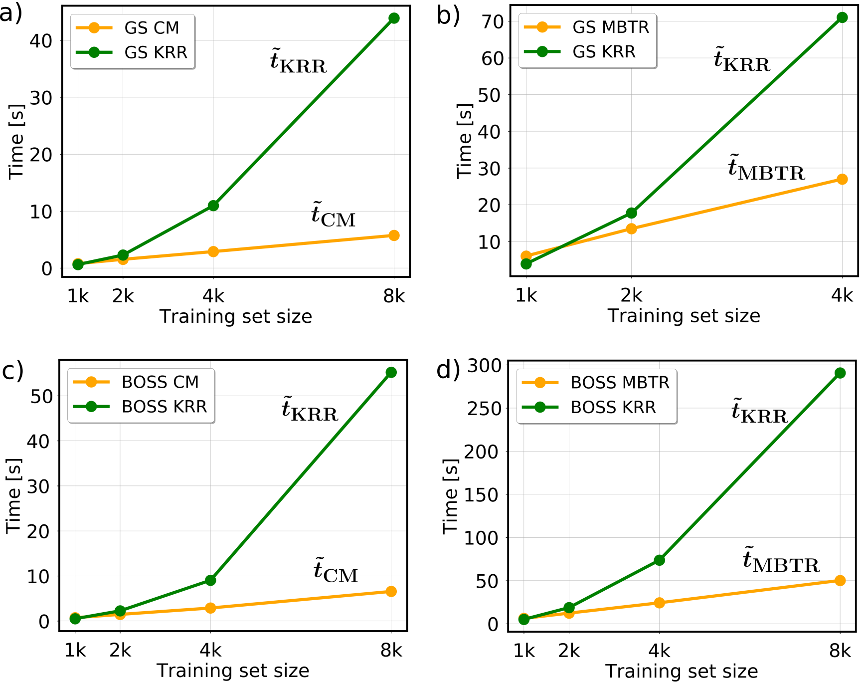
Figure 10: Comparison between average times (per iteration) needed to perform 5-fold cross-validated KRR ($\widetilde{t}_{\textnormal{KRR}}$) and to build the molecular descriptor ($\widetilde{t}_{\textnormal{CM}}$ or $\widetilde{t}_{\textnormal{MBTR}}$). In a) and b), timings are shown for grid search (GS) and in c) and d) for BOSS. Panels a) and c) are for the CM (2D search) and b) and d) for the MBTR (4D search). Note that for the MBTR, grid search is only performed for training set sizes up to 4k.

To collect run time information we added timing statements to our KRR implementation. Figure 10 depicts the average time the BOSS and grid search algorithms need to build the molecular descriptor and run cross-validated KRR, as a function of training set size for KRR-CM and KRR-MBTR. Panels a) and b) show the timings for grid search and panels c) and d) for BOSS. We observe that our formal scaling estimates in the previous section are confirmed, as the average time for building the CM ($\widetilde{t}_{\textnormal{CM}}$) or the MBTR ($\widetilde{t}_{\textnormal{MBTR}}$) grow linearly with training set size, while $\widetilde{t}_{\textnormal{KRR}}$ grows cubically with training set size. Hence, for the smallest training set size of 1k, it might take less time to perform KRR than to build the molecular descriptor, while for training set sizes of 2k and larger the cubic scaling of the KRR part has already overtaken the descriptor building.

The total computing time as a function of training set size is presented in Fig. 11. In the 2D case the grid search outperforms BOSS, while in the 4D case, BOSS is significantly faster than grid search. To determine which approach is faster – grid search or BOSS – it comes down to how often the descriptor has to be build, $n_{\textnormal{desc}}$, in each method and how often cross-validated KRR has to be performed, $n_{\textnormal{KRR}}$. Table 3 shows both numbers for grid search and BOSS. In grid search, $n_{\textnormal{desc}}$ and $n_{\textnormal{KRR}}$ are fixed numbers (see Algorithms 1 and 2). They depend only on the size of the hyperparameter grid. In KRR-CM, the CM needs to be computed only once at the beginning of the routine. Cross-validated KRR is performed 121 times, for each combination of $\alpha$ and $\gamma$. In a 4D KRR-MBTR grid search, the MBTR needs to be computed for each combination of $\sigma_{2}$ and $\sigma_{3}$, i.e. 36 times. Cross-validated KRR is performed for each possible combination of $\alpha$, $\gamma$, $\sigma_{2}$ and $\sigma_{3}$, i.e. 4,356 times.

In BOSS, the molecular descriptor must be built and cross-validated KRR must be performed every single time the objective function is evaluated, as shown in Algorithms 3 and 4. This means that $n_{\textnormal{desc}}$ and $n_{\textnormal{KRR}}$ solely depend on the number of BOSS iterations required to converge the MAE landscapes.

Since $\widetilde{t}_{\textnormal{KRR}}$ scales cubically, the critical number is $n_{\textnormal{KRR}}$. As Tab. 3 illustrates, $n_{\textnormal{KRR}}$ are roughly the same for grid search and BOSS in the 2D search. Already for a 4D search, BOSS requires significantly fewer KRR evaluations than grid search and is computationally much more efficient.

	2D (CM)		4D (MBTR)
	GS	BOSS	GS	BOSS
$\bm{n}_{\textnormal{desc}}$	1	100	36	300
$\bm{n}_{\textnormal{KRR}}$	121	100	4,356	300

Table 3: Number of times the molecular descriptor is built ($n_{\textnormal{desc}}$) and cross-validated KRR is performed ($n_{\textnormal{KRR}}$), using the grid search (GS) and BOSS approaches.

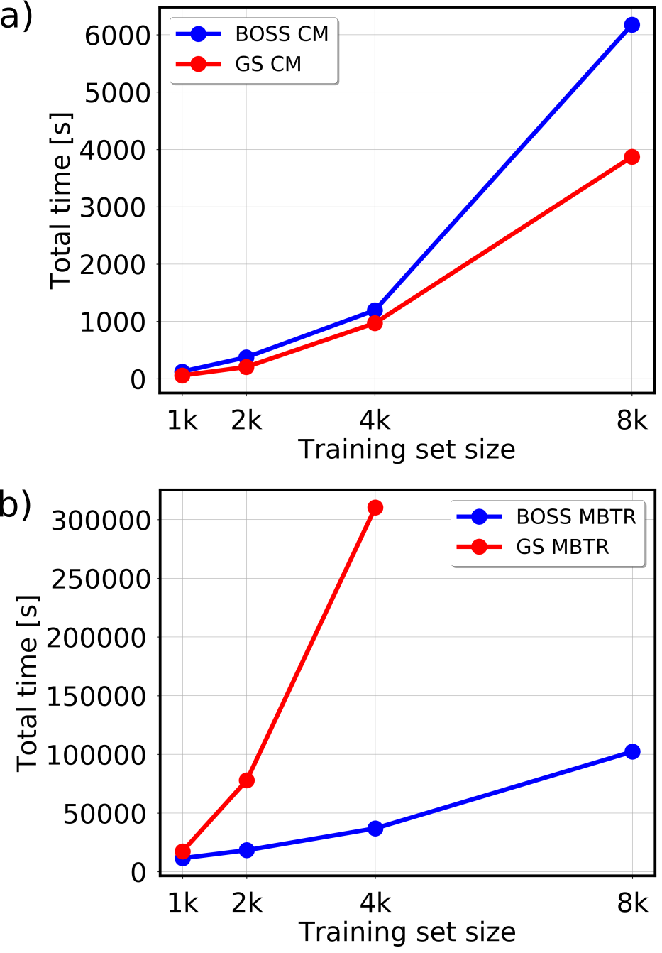
Figure 11: Total times for hyperparameter optimization by BOSS and grid search as a function of training set size. In a) the CM and in b) the MBTR is used as molecular descriptor. Timings are shown for optimization on the QM9 dataset. For grid search (GS), only training set sizes up to 4k are feasable to be considered.

			QM9		AA		OE
descriptor	hyperparam.	train size	BOSS	GS	BOSS	GS	BOSS	GS
CM	$\alpha$, $\gamma$	1k	0.300 [0.302]	0.304	0.829 [0.812]	0.843	0.355 [0.357]	0.368
CM	$\alpha$, $\gamma$	2k	0.269 [0.270]	0.277	0.645 [0.651]	0.658	0.353 [0.350]	0.355
CM	$\alpha$, $\gamma$	4k	0.237 [0.238]	0.244	0.507 [0.508]	0.509	0.332 [0.335]	0.338
CM	$\alpha$, $\gamma$	8k	0.212 [0.211]	0.215	0.373 [0.374]	0.382	0.303 [0.305]	0.309
MBTR	$\alpha$, $\gamma$, $\sigma_{2}$, $\sigma_{3}$	1k	0.207 [0.212]	0.214	0.464 [0.466]	0.500	0.246 [0.243]	0.246
MBTR	$\alpha$, $\gamma$, $\sigma_{2}$, $\sigma_{3}$	2k	0.190 [0.165]	0.190	0.338 [0.348]	0.361	0.233 [0.231]	0.227
MBTR	$\alpha$, $\gamma$, $\sigma_{2}$, $\sigma_{3}$	4k	0.159 [0.162]	0.166	0.334 [0.276]	0.296	0.216 [0.218]	0.219
MBTR	$\alpha$, $\gamma$, $\sigma_{2}$, $\sigma_{3}$	8k	0.142 [0.149]	–	0.213 [0.214]	–	0.189 [0.184]	–

Table 4: MAEs [eV] for the optimal set of hyperparameter found by BOSS and grid search (GS). Results are depicted for three different molecular datasets QM9, AA and OE. For BOSS, the first value is the best ever observed true function value f($\bm{\hat{z}}$), evaluated at the predicted optimal point $\bm{\hat{z}}$. The second value in squared brackets is the global minimum predicted by the surrogate model, $\mu(\bm{\hat{z}})$, at maximum number of iterations. For GS, the depicted value corresponds to the best model performance $f(\bm{\hat{z}})$.

IV Conclusion

In this work, we have used the Bayesian optimization tool BOSS to optimize hyperparameters in a KRR machine-learning model that predicts molecular orbital energies. We use two different molecular descriptors, the CM and the MBTR. While the CM has no hyperparameters, the MBTR molecular descriptor introduces two extra hyperparameters to the optimization problem. We therefore performed BOSS searches in spaces of up to four dimensions. We compared MAE landscapes in hyperparameter space and the efficiency of the BOSS approach with the commonly used grid search approach for three different molecular datasets.

For CM as molecular descriptor, only the two KRR hyperparameters $\alpha$ and $\gamma$ need to be optimized. The 2D landscapes in hyperparameter space produced by BOSS and grid search agree very well, with the lowest MAE values lying on a diagonal and a horizontal line. This is the case for all three datasets and for all training set sizes.

For MBTR as molecular descriptor, MAE landscapes cut through the (log($\alpha$), log($\gamma$))-plane qualitatively correspond to the MAE landscapes of the 2D optimization problem, while the overall prediction errors are notably lower. In the ($\sigma_{2}$, $\sigma_{3}$)-plane, the optimal MAE values are confined to a small, roughly spherical region. The MAE is not very sensitive to $\sigma_{2}$ and $\sigma_{3}$, in contrast to $\alpha$ and $\gamma$. Hence, all combinations of $\sigma_{2}$ and $\sigma_{3}$ are reasonable choices for the MBTR.

In terms of efficiency, grid search outperforms BOSS in the 2D case, while in the 4D case, BOSS is significantly faster than grid search. This paves the way for high-dimensional hyperparameter optimization with Bayesian optimization.

References

Appendix A Tables

QM9		log($\alpha$)		log($\gamma$)		log($\sigma_{2}$)		log($\sigma_{3}$)		$\mu(\bm{\hat{z}})$	$f(\bm{\hat{z}})$
descriptor	train size	BOSS	GS	BOSS	GS	BOSS	GS	BOSS	GS	BOSS	GS
CM	1k	-8.0	-3.0	-3.0	-3.0	–	–	–	–	0.302	0.304
CM	2k	-6.7	-10.0	-3.3	-3.0	–	–	–	–	0.270	0.277
CM	4k	-2.0	-10.0	-3.5	-3.0	–	–	–	–	0.238	0.244
CM	8k	-10.0	-10.0	-3.4	-3.0	–	–	–	–	0.211	0.215
MBTR	1k	-2.1	-2.0	-1.0	-1.0	-1.8	-2.0	-1.2	-2.0	0.212	0.214
MBTR	2k	-3.1	-3.0	-1.0	-1.0	-1.1	-2.0	-1.9	-1.0	0.165	0.190
MBTR	4k	-2.3	-2.0	-3.9	-1.0	-1.5	-5.0	-1.3	-3.0	0.162	0.166
MBTR	8k	-1.6	–	0.0	–	-1.6	–	-1.1	–	0.149	–

Table 5: Optimal hyperparameters $\bm{\hat{z}}$ and corresponding best model performance $f(\bm{\hat{z}})$ for the QM9 dataset, computed by BOSS and grid search (GS).

AA		log($\alpha$)		log($\gamma$)		log($\sigma_{2}$)		log($\sigma_{3}$)		$\mu(\bm{\hat{z}})$	$f(\bm{\hat{z}})$
descriptor	train size	BOSS	GS	BOSS	GS	BOSS	GS	BOSS	GS	BOSS	GS
CM	1k	-4.1	-10.0	-4.0	-4.0	–	–	–	–	0.812	0.843
CM	2k	-1.0	-10.0	-3.9	-4.0	–	–	–	–	0.651	0.658
CM	4k	-4.8	-10.0	-3.7	-4.0	–	–	–	–	0.508	0.509
CM	8k	-6.5	-10.0	-3.8	-4.0	–	–	–	–	0.374	0.382
MBTR	1k	-3.1	-4.0	-1.7	0.0	-1.0	-1.0	0.0	0.0	0.466	0.500
MBTR	2k	-3.8	-4.0	-1.9	0.0	-1.5	-1.0	-4.0	0.0	0.348	0.361
MBTR	4k	-9.2	-5.0	-2.6	0.0	-1.1	-1.0	0.0	0.0	0.276	0.296
MBTR	8k	-3.3	–	0	–	-1.8	–	-0.3	–	0.214	–

Table 6: Optimal hyperparameters $\bm{\hat{z}}$ and corresponding best model performance $f(\bm{\hat{z}})$ for the AA dataset, computed by BOSS and grid search (GS).

OE		log($\alpha$)		log($\gamma$)		log($\sigma_{2}$)		log($\sigma_{3}$)		$\mu(\bm{\hat{z}})$	$f(\bm{\hat{z}})$
descriptor	train size	BOSS	GS	BOSS	GS	BOSS	GS	BOSS	GS	BOSS	GS
CM	1k	-3.0	-6.0	-6.7	-10.0	–	–	–	–	0.357	0.368
CM	2k	-1.6	-5.0	-4.7	-9.0	–	–	–	–	0.350	0.355
CM	4k	-1.2	-1.0	-4.4	-5.0	–	–	–	–	0.335	0.338
CM	8k	-1.4	-6.0	-4.4	-10.0	–	–	–	–	0.305	0.309
MBTR	1k	-1.8	-2.0	-1.0	-1.0	-2.6	-2.0	-5.0	-1.0	0.243	0.246
MBTR	2k	-2.2	-2.0	-1.1	-1.0	-2.6	-2.0	-1.1	-2.0	0.231	0.227
MBTR	4k	-1.8	-2.0	-1.0	-1.0	-2.8	-3.0	-1.2	-2.0	0.218	0.219
MBTR	8k	-2.6	–	-1.3	–	-5.0	–	-3.6	–	0.184	–

Table 7: Optimal hyperparameters $\bm{\hat{z}}$ and corresponding best model performance $f(\bm{\hat{z}})$ for the OE dataset, computed by BOSS and grid search (GS).

References

- (1) DScribe. https://github.com/SINGROUP/dscribe. Accessed: 2018-11-21.
- (2) A. Agrawal and A. Choudhary. Perspective: Materials informatics and big data: Realization of the “fourth paradigm” of science in materials science. APL Mater., 4(5):053208, Apr. 2016.
- (3) M. Aykol, J. S. Hummelshøj, A. Anapolsky, K. Aoyagi, M. Z. Bazant, T. Bligaard, R. D. Braatz, S. Broderick, D. Cogswell, J. Dagdelen, W. Drisdell, E. Garcia, K. Garikipati, V. Gavini, W. E. Gent, L. Giordano, C. P. Gomes, R. Gomez-Bombarelli, C. Balaji Gopal, J. M. Gregoire, J. C. Grossman, P. Herring, L. Hung, T. F. Jaramillo, L. King, H.-K. Kwon, R. Maekawa, A. M. Minor, J. H. Montoya, T. Mueller, C. Ophus, K. Rajan, R. Ramprasad, B. Rohr, D. Schweigert, Y. Shao-Horn, Y. Suga, S. K. Suram, V. Viswanathan, J. F. Whitacre, A. P. Willard, O. Wodo, C. Wolverton, and B. D. Storey. The materials research platform: Defining the requirements from user stories. Matter, 1(6):1433–1438, Dec 2019.
- (4) C. W. Coley, N. S. Eyke, and K. F. Jensen. Autonomous discovery in the chemical sciences part ii: Outlook. Angewandte Chemie International Edition, n/a(n/a).
- (5) D. Dua and C. Graff, 2017.
- (6) B. R. Goldsmith, J. Esterhuizen, J.-X. Liu, C. J. Bartel, and C. Sutton. Machine learning for heterogeneous catalyst design and discovery. AIChE Journal, 64(7):2311–2323, 2018.
- (7) R. Gómez-Bombarelli, J. Aguilera-Iparraguirre, T. D. Hirzel, D. Duvenaud, D. Maclaurin, M. A. Blood-Forsythe, H. S. Chae, M. Einzinger, D.-G. Ha, T. C.-C. Wu, G. Markopoulos, S. Jeon, H. Kang, H. Miyazaki, M. Numata, S. Kim, W. Huang, S. I. Hong, M. A. Baldo, R. P. Adams, and A. Aspuru-Guzik. Design of efficient molecular organic light-emitting diodes by a high-throughput virtual screening and experimental approach. Nature materials, 15 10:1120–7, 08 2016.
- (8) G. H. Gu, J. Noh, I. Kim, and Y. Jung. Machine learning for renewable energy materials. J. Mater. Chem. A, 2019.
- (9) M. U. Gutmann and J. Corander. Bayesian optimization for likelihood-free inference of simulator-based statistical models. Journal of Machine Learning Research, 17(125):1–47, 2016.
- (10) T. Hey, S. Tansley, and K. Tolle. The Fourth Paradigm: Data-Intensive Scientific Discovery. Microsoft Research, Redmond, WA, USA, 2009.
- (11) L. Himanen, A. Geurts, A. S. Foster, and P. Rinke. Data-driven materials science: Status, challenges, and perspectives. Adv. Sci., 6(21):1900808, 2019.
- (12) H. Huo and M. Rupp. Unified Representation for Machine Learning of Molecules and Crystals. arXiv:1704.06439 [cond-mat, physics:physics], Apr. 2017. arXiv: 1704.06439.
- (13) K. F. Jensen, C. W. Coley, and N. S. Eyke. Autonomous discovery in the chemical sciences part i: Progress. Angewandte Chemie International Edition, n/a(n/a).
- (14) J. Ma, R. P. Sheridan, A. Liaw, G. E. Dahl, and V. Svetnik. Deep neural nets as a method for quantitative structure–activity relationships. Journal of Chemical Information and Modeling, 55(2):263–274, 2015. PMID: 25635324.
- (15) B. Meyer, B. Sawatlon, S. Heinen, O. A. von Lilienfeld, and C. Corminboeuf. Machine learning meets volcano plots: computational discovery of cross-coupling catalysts. Chem. Sci., 9:7069–7077, 2018.
- (16) T. Müller, A. G. Kusne, and R. Ramprasad. Machine Learning in Materials Science, chapter 4, pages 186–273. John Wiley & Sons, Ltd, Hoboken, New Jersey, USA, 2016.
- (17) R. S. Olson, N. Bartley, R. J. Urbanowicz, and J. H. Moore. Evaluation of a tree-based pipeline optimization tool for automating data science. In Proceedings of the Genetic and Evolutionary Computation Conference 2016, GECCO ’16, page 485–492, New York, NY, USA, 2016. Association for Computing Machinery.
- (18) V. Perrone, H. Shen, M. Seeger, C. Archambeau, and R. Jenatton. Learning search spaces for bayesian optimization: Another view of hyperparameter transfer learning. In NeurIPS, 2019.
- (19) R. Ramakrishnan, P. O. Dral, M. Rupp, and O. A. von Lilienfeld. Quantum chemistry structures and properties of 134 kilo molecules. Scientific Data, 1, 2014.
- (20) C. E. Rasmussen and C. K. I. Williams. Gaussian Processes for Machine Learning. The MIT Press, 2006.
- (21) M. Ropo, M. Schneider, C. Baldauf, and V. Blum. First-principles data set of 45,892 isolated and cation-coordinated conformers of 20 proteinogenic amino acids. Scientific Data, 3, 2 2016.
- (22) M. Rupp, A. Tkatchenko, K.-R. Müller, and O. A. von Lilienfeld. Fast and Accurate Modeling of Molecular Atomization Energies with Machine Learning. Physical Review Letters, 108(5):058301, Jan. 2012.
- (23) M. Rupp, O. A. von Lilienfeld, and K. Burke. Guest editorial: Special topic on data-enabled theoretical chemistry. Journal of Chemical Physics, 148(24):241401, 2018.
- (24) J. Schmidt, M. R. G. Marques, S. Botti, and M. A. L. Marques. Recent advances and applications of machine learning in solid-state materials science. npj Computational Materials, 5(1):83, 2019.
- (25) A. D. Sendek, E. D. Cubuk, E. R. Antoniuk, G. Cheon, Y. Cui, and E. J. Reed. Machine learning-assisted discovery of many new solid li-ion conducting materials. Technical Report arXiv:1808.02470 [cond-mat.mtrl-sci], ArXiV, August 2018.
- (26) M. A. Shandiz and R. Gauvin. Application of machine learning methods for the prediction of crystal system of cathode materials in lithium-ion batteries. Computational Materials Science, 117:270 – 278, 2016.
- (27) N. Srinivas, A. Krause, S. Kakade, and M. Seeger. Gaussian process optimization in the bandit setting: No regret and experimental design. In Proceedings of the 27th International Conference on International Conference on Machine Learning, ICML 2010, pages 1015–1022, Madison, WI, USA, 2010. Omnipress.
- (28) A. Stuke, C. Kunkel, D. Golze, M. Todorovic, J. T. Margraf, K. Reuter, P. Rinke, and H. Oberhofer. Atomic structures and orbital energies of 61,489 crystal-forming organic molecules. Scientific Data, 7(1):58, 2020.
- (29) A. Stuke, M. Todorović, M. Rupp, C. Kunkel, K. Ghosh, L. Himanen, and P. Rinke. Chemical diversity in molecular orbital energy predictions with kernel ridge regression. J. Chem. Phys., 150(20):204121, 2019.
- (30) The Minerals Metals & Materials Society (TMS). Building a Materials Data Infrastructure: Opening New Pathways to Discovery and Innovation in Science and Engineering. TMS, Pittsburgh, PA, USA, 2017.
- (31) M. Todorović, M. U. Gutmann, J. Corander, and P. Rinke. Bayesian inference of atomistic structure in functional materials. npj Comp. Mat., 5(1):35, 2019.
- (32) J. Wu, X.-Y. Chen, H. Zhang, L.-D. Xiong, H. Lei, and S.-H. Deng. Hyperparameter optimization for machine learning models based on bayesian optimizationb. Journal of Electronic Science and Technology, 17(1):26 – 40, 2019.
- (33) D. Yogatama and G. Mann. Efficient transfer learning method for automatic hyperparameter tuning. In AISTATS, 2014.
- (34) M. T. Young, J. Hinkle, A. Ramanathan, and R. Kannan. "hyperspace: Distributed bayesian hyperparameter optimization". In Proceedings of the Genetic and Evolutionary Computation Conference 2016, pages 339–347. 30th International Symposium on Computer Architecture and High Performance Computing (SBAC-PAD), 2018.
- (35) A. Zunger. Inverse design in search of materials with target functionalities. Nat. Rev. Chem., 2:0121, Mar 2018.