Generating primordial features at large scales in two field models of inflation

Abstract

We investigate the generation of features at large scales in the primordial power spectrum (PPS) when inflation is driven by two scalar fields. In canonical single field models of inflation, these features are often generated due to deviations from the slow-roll regime. While deviations from slow-roll can be naturally achieved in two field models due to a sharp turn in the trajectory in the field space, features at the largest scales of the types suggested by CMB temperature anisotropies are more difficult to achieve in models involving two canonical scalar fields due to the presence of isocurvature fluctuations. We show instead that a coupling between the kinetic terms of the scalar fields can easily produce such features. We discuss models whose theoretical predictions are consistent with current observations and highlight the implications of our results.

1 Introduction

The measurements of anisotropies in the Cosmic Microwave Background (CMB) point to a primordial power spectrum (PPS) of adiabatic nearly Gaussian scalar fluctuations whose deviation from scale invariance has been accurately measured  [1, 2]. The most effective and compelling paradigm to generate perturbations of such type is slow-roll inflation and, in fact, there exist many inflationary models that are remarkably consistent with the cosmological data [1]. However, it has been shown by different methodologies that deviations from the simple power-law in the PPS which is predicted by slow-roll inflation to leading order, can lead to an improvement in the fit to CMB anisotropies, although not at a statistically significant level [1]. Reconstructions of primordial power spectrum directly from CMB data have been indicating features in several publications [3, 4, 5, 6, 7, 8, 9, 10, 11, 12, 13, 14, 15, 16, 17, 18, 19].

These features can be broadly divided into the following three types: a lack of power at large scales [20, 21, 22, 23, 24, 25, 26, 27, 28, 29, 30, 31, 32, 33, 34, 35, 36, 37, 38], a dip and burst of oscillations around multipoles $\ell=20$–$40$ [39, 40, 41, 42, 43, 44, 45, 46, 47], and smaller oscillations that persist from intermediate to the smallest scales [48, 49, 50, 51, 52, 53, 54, 55, 56, 57, 58, 59, 60, 61, 62, 63, 64].

In the simplest inflationary models involving a single, canonical scalar field, features in the power spectrum are generated by a departure from the slow-roll regime or from Bunch-Davies initial conditions. The departures from the slow-roll regime, in turn, are often achieved by specific features in the inflaton potential, such as a point of inflection, a step or oscillatory terms. There has been a constant effort in the literature to construct inflationary models that naturally lead to features in the scalar power spectrum.

Inflation driven by two or more scalar fields offer a richer dynamics and phenomenology (see [65] for a review). With more than one field, there are several possibilities to produce features in the PPS, as first pointed out in  [66]. Beyond introducing features in the potential for the inflatons [67], other phenomena are at play, such as particle production of additional spectator (i.e. with zero vev) fields coupled to the inflaton [68], couplings to gravity [69, 70, 71] or a turn in the trajectory in field space. Features originating from a turn in the trajectory in field space have been studied explicitly including curvature and isocurvature perturbations [72] or in an effective single field approach by integrating out heavy degrees of freedom [73].

In this paper we adopt the approach of a direct integration of two-field dynamics with turns in field space, trying to avoid complicated forms, such as allowing transitions, steps or cutoffs in the effective potential. Indeed, in two field models, deviations from slow-roll can be achieved between two different stages of inflation, as in double inflation [74], and this is the case we will focus on. The possible connection between two field inflation and features at the largest scales has been already made in [75]. However, differently from [75], we demonstrate that a step-like feature with a higher amplitude on large scales is obtained when isocurvature perturbations are correctly taken into account, which is not so interesting from an observational point of view for CMB temperature anisotropies.

We therefore study the generation of features in a two field model consisting of a canonical scalar field (say, $\phi$) and a second scalar field (say, $\chi$) with a non-canonical kinetic term of the form $f(\phi)(\partial\chi)^{2}$. For works on two field inflation with these non-canonical kinetic terms - not necessarily connected to features - see for example [76, 77, 78, 79, 80, 81, 82]. Thereby, we focus on a setting in which $\phi$ ($\chi$) is the effectively heavier (lighter) field driving the first (second) stage of inflation. Since the deviations from slow-roll do not permit in general analytical calculations, we therefore use complete numerical computations to determine the primordial power spectra by evolving both background and perturbations. We show that the effective mass of isocurvature perturbations grows with the coupling $f(\phi)$ during the first stage of inflation. Therefore, when isocurvature perturbations cross the Hubble radius, they decay and the feedback to curvature perturbation is thus suppressed. This effect reduces the correlation between the curvature and the isocurvature perturbation in a way that a suppression of power is achieved for scales that cross the Hubble radius before the temporary violation of the slow-roll conditions, that is during the first stage of inflation.

This paper is organized as follows. In the following section, we describe the model of our interest and summarize the equations governing the background and the perturbations. In Sec. 2, we outline the numerical procedure that we adopt to evolve the background and the perturbations. In particular, we describe in Sec. 3 the important role isocurvature perturbations play in our analysis. In Sec. 4, we then introduce our toy model and present the results of our numerical computation for the PPS for a large range of scales and comment on the role of the different parameters at play in generating relevant features. We then discuss the two cases when scales relevant to CMB anisotropies observations cross the Hubble radius during or well before the slow-roll violation in Sec. 5. In Appendix A, for completeness, we provide an additional scan of the parameter space for the model presented in Sec. 5.

2 Theoretical construction

In this section, we review the formalism essential to study the generation of perturbations in two field models of inflation with a coupling between the kinetic terms in terms of tangent and orthogonal field  [83, 84, 80, 81].

2.1 Background Dynamics

We consider a model consisting of two scalar fields, say, $\phi$ and $\chi$, whose dynamics is governed by the following action:

$$S[\phi,\chi]=\int{\rm d}^{4}x\,\sqrt{-g}\,\left[\frac{{M_{{}_{\textup{Pl}}}}^{2}}{2}R-\frac{1}{2}(\partial\phi)^{2}-\frac{f(\phi)}{2}(\partial\chi)^{2}-V(\phi,\chi)\right].$$ (2.1)

Note that, while $\phi$ is a canonical scalar field, $\chi$ is a non-canonical scalar field due to the presence of the function $f(\phi)$ in the term describing its kinetic energy. Evidently, apart from the potential $V(\phi,\chi)$, through which the fields can in principle interact, the function $f(\phi)$ also leads to an interaction between the fields. In order to connect with the equations of Refs. [80, 81] we define $f(\phi)\equiv{\rm e}^{2b(\phi)}$.

We work with the spatially flat Friedmann-Lemaître-Robertson-Walker (FLRW) universe described by the line-element

$${\rm d}s^{2}=-{\rm d}t^{2}+a^{2}(t)\,{\rm d}{\bm{x}}^{2},$$ (2.2)

where $a(t)$ is the scale factor and $t$ is the cosmic time. In such a smooth background, the equations of motion governing the homogeneous scalar fields are given by

$$\ddot{\phi}+3H\dot{\phi}+V_{\phi} = b_{\phi}e^{2b}\dot{\chi}^{2},$$ (2.3a)

$$\ddot{\chi}+(3H+2b_{\phi}\dot{\phi})\dot{\chi}+{\rm e}^{-2b}V_{\chi} = 0,$$ (2.3b)

where, as usual, the overdots represent differentiation with respect to the cosmic time, $H=\dot{a}/a$ is the Hubble parameter, while the subscripts denote differentation of the potential $V(\phi,\chi)$ and the function $b(\phi)$ with respect to the corresponding fields. The dynamics of the scale factor is described by the following Friedmann equations:

$$H^{2} = \frac{1}{3{M_{{}_{\textup{Pl}}}}^{2}}\left[\frac{\dot{\phi}^{2}}{2}+{\rm e}^{2b}\frac{\dot{\chi}^{2}}{2}+V\right],$$ (2.4a)

$$\dot{H} = -\frac{1}{2{M_{{}_{\textup{Pl}}}}^{2}}\left[\dot{\phi}^{2}+{\rm e}^{2b}\dot{\chi}^{2}\right].$$ (2.4b)

To characterize the evolution of the background, it is useful to introduce the so-called Hubble Flow Functions (HFFs) as follows [85]:

$$\epsilon_{i+1}\equiv\frac{{\rm d}\ln\epsilon_{i}}{{\rm d}N},$$ (2.5)

with

$$\epsilon_{0}\equiv\frac{H_{\textup{\rm in}}}{H}$$ (2.6)

where $H_{\rm in}$ is the value of the Hubble parameter at some initial time during inflation, and $N=\int{\rm d}tH$ represents the number of e-folds. The HFFs hierarchy is not only useful to define a successful slow-roll regime (i.e. $\epsilon_{1}\,,\epsilon_{2}\ll 1$) or the end of inflation ($\epsilon_{1}=1$), but also to quantify violations of the slow-roll regime which are of particular interest for this paper.

2.2 Linear Perturbations

Let us now turn to the dynamics of perturbations around the homogeneous vev of the scalar fields. To describe the scalar perturbations, for simplicity, we work in the Newtonian gauge. Since scalar fields do not have anisotropic stress to linear order, in the Newtonian gauge, the perturbed FRLW metric takes the form [86]

$${\rm d}s^{2}=-(1+2\Phi)\,{\rm d}t^{2}+a^{2}(t)\,(1-2\Phi)\,{\rm d}{\bm{x}}^{2}\,,$$ (2.7)

where $\Phi$ is the Bardeen potential characterizing the perturbations.

To study the evolution of the perturbations, it proves to be convenient to decompose the perturbations in the scalar fields, say, $\delta\phi$ and $\delta\chi$, along directions that are parallel and orthogonal directions to the trajectory in the field space [83]. These correspond to the instantaneous adiabatic and isocurvature perturbations and they are given by the expressions [80]

$$\delta\sigma = \cos\theta\,\delta\phi+\sin\theta\,{\rm e}^{b}\,\delta\chi,$$ (2.8a)

$$\delta s = -\sin\theta\,\delta\phi+\cos\theta\,{\rm e}^{b}\,\delta\chi,$$ (2.8b)

with the quantity $\theta$ being an angle in the field space that is defined through the relations

$$\cos\theta=\frac{\dot{\phi}}{\dot{\sigma}},\quad\sin\theta={\rm e}^{b}\frac{\dot{\chi}}{\dot{\sigma}},\quad\dot{\sigma}^{2}=\dot{\phi}^{2}+{\rm e}^{2b}\dot{\chi}^{2}.$$ (2.9)

The equations (2.3) describing background scalar fields can be combined to arrive at the following equations governing $\dot{\sigma}$ and the angle $\theta$:

$$\ddot{\sigma}+3H\dot{\sigma}+V_{\sigma} = 0,$$ (2.10a)

$$\dot{\theta} = -\frac{V_{s}}{\dot{\sigma}}-b_{\phi}\dot{\sigma}\sin\theta$$ (2.10b)

where $V_{\sigma}$ and $V_{s}$ are given by

$$V_{\sigma} = V_{\phi}\cos\theta+{\rm e}^{-b}\,V_{\chi}\sin\theta,$$ (2.11a)

$$V_{s} = -V_{\phi}\sin\theta+{\rm e}^{-b}\,V_{\chi}\cos\theta.$$ (2.11b)

We also introduce here the following quantities for future convenience

$$V_{\sigma\sigma} = V_{\phi\phi}\cos^{2}\theta+{\rm e}^{-b}V_{\phi\chi}\sin 2\theta+{\rm e}^{-2b}V_{\chi\chi}\sin^{2}\theta,$$ (2.12a)

$$V_{ss} = V_{\phi\phi}\sin^{2}\theta-{\rm e}^{-b}V_{\phi\chi}\sin 2\theta+{\rm e}^{-2b}V_{\chi\chi}\cos^{2}\theta,$$ (2.12b)

$$V_{\sigma s} = -V_{\phi\phi}\cos\theta\sin\theta+{\rm e}^{-b}V_{\phi\chi}(\cos^{2}\theta-\sin^{2}\theta)+{\rm e}^{-2b}V_{\chi\chi}\cos\theta\sin\theta.$$ (2.12c)

To characterize the perturbations, we consider the gauge-invariant Mukhanov-Sasaki variable $Q_{\sigma}$ associated to $\delta\sigma$, i.e. $Q_{\sigma}=\delta\sigma+\dot{\sigma}/H\Phi$, and $\delta s$ (which is already gauge-invariant), associated with the adiabatic and isocurvature fields. The equations of motion governing $Q_{\sigma}$ and $\delta s$ can be arrived at from the differential equations describing the perturbations in the scalar fields and the first order Einstein’s equations. They can be obtained to be

$$\ddot{Q}_{\sigma}+3H\dot{Q}_{\sigma} + \left[\frac{k^{2}}{a^{2}}+V_{\sigma\sigma}-\dot{\theta}^{2}-\frac{1}{a^{3}{M_{{}_{\textup{Pl}}}}^{2}}\left(\frac{a^{3}\dot{\sigma}^{2}}{H}\right)^{\raisebox{0.75346pt}{ \leavevmode\hbox to1.2pt{\vbox to1.2pt{\text{[drawing]}}}}}+b_{\phi}u(t)\right]Q_{\sigma}$$ (2.13a)

$$= 2\left(\dot{\theta}\delta s\right)^{\raisebox{0.75346pt}{ \leavevmode\hbox to1.2pt{\vbox to1.2pt{\text{[drawing]}}}}}-2\left(\frac{\dot{H}}{H}+\frac{V_{\sigma}}{\dot{\sigma}}\right)\dot{\theta}\delta s+b_{\phi\phi}\dot{\sigma}^{2}\sin 2\theta\delta s+2b_{\phi}h(t)\,,\qquad$$

$$\ddot{\delta s}+3H\dot{\delta s} + \left[\frac{k^{2}}{a^{2}}+V_{ss}+3\dot{\theta}^{2}+b^{2}_{\phi}g(t)+b_{\phi}f(t)-b_{\phi\phi}\dot{\sigma}^{2}-4\frac{V_{s}^{2}}{\dot{\sigma}^{2}}\right]\delta s$$ (2.13b)

$$= 2\frac{V_{s}}{H}\left(\frac{H}{\dot{\sigma}}Q_{\sigma}\right)^{\raisebox{0.75346pt}{ \leavevmode\hbox to1.2pt{\vbox to1.2pt{\text{[drawing]}}}}},$$

where the quantities $u(t)$, $h(t)$, $g(t)$ and $f(t)$ are given by

$$u(t) = \dot{\theta}\dot{\sigma}\sin\theta-{\rm e}^{-b}V_{\chi}\sin\theta\cos\theta,$$ (2.14a)

$$h(t) = -\dot{\sigma}(\sin\theta\,\delta s)^{\raisebox{0.75346pt}{ \leavevmode\hbox to1.2pt{\vbox to1.2pt{\text{[drawing]}}}}}-\sin\theta\left(\frac{\dot{H}}{H}\dot{\sigma}+2V_{\sigma}\right)\delta s-3H\dot{\sigma}\sin\theta\delta s,$$ (2.14b)

$$g(t) = -\dot{\sigma}^{2}(1+3\sin^{2}\theta),$$ (2.14c)

$$f(t) = V_{\phi}(1+\sin^{2}\theta)-4V_{s}\sin\theta.$$ (2.14d)

We choose to impose the following Bunch-Davies initial conditions on the variables $Q_{\sigma}$ and $\delta s$ at early times when the modes of cosmological interest are well inside the Hubble radius:

$$Q_{\sigma}(\tau)\simeq\delta s(\tau)\simeq\frac{1}{a(\tau)}\,\frac{{\rm e}^{\imath k\tau}}{\sqrt{2k}},$$ (2.15)

where $\tau$ is the conformal time coordinate defined as $\tau=\int\,{\rm d}t/a(t)$. We have verified that the same results are obtained by considering Bunch-Davies initial conditions for the gauge-invariant variables associated to $\phi$ and $\chi$ instead. Note, however, that extra care is needed when imposing the initial conditions in case the turning rate, i.e. $\dot{\theta}$, is not small and $Q_{\sigma}$ and $\delta_{s}$ can be correlated at early times [87].

While $Q_{\sigma}$ and $\delta s$ are convenient variables to identify the most natural initial conditions that can be imposed, it is also useful to think in terms of curvature and isocurvature fluctuations, which are used to classify initial conditions in the post-inflationary expansion. These quantities are given in terms of the variables $Q_{\sigma}$ and $\delta s$ by the following relations:

$$\mathcal{R}=\frac{H}{\dot{\sigma}}Q_{\sigma},\quad\mathcal{S}=\frac{H}{\dot{\sigma}}\delta s.$$ (2.16)

Upon utilizing the equations (2.13), it is straightforward to arrive at the following equations governing the curvature and the isocurvature perturbations ${\mathcal{R}}$ and ${\mathcal{S}}$:

$$\ddot{\mathcal{R}} + \left(H+2\frac{\dot{z}}{z}\right)\dot{\mathcal{R}}+\frac{k^{2}}{a^{2}}\mathcal{R}=-\frac{2V_{s}}{\dot{\sigma}}\dot{\mathcal{S}}-\,2\biggl{(}-{\rm e}^{-b}b_{\phi}\cos^{2}\theta\,V_{\chi}+\sin\theta b_{\phi}V_{\sigma}$$ (2.17a)

$$\qquad\qquad\qquad\qquad\qquad\;\;+\,V_{\sigma s}+\frac{\dot{\sigma}}{HM^{2}_{\textup{pl}}}V_{s}\biggr{)}\mathcal{S},$$

$$\ddot{\mathcal{S}} + \left(H+2\frac{\dot{z}}{z}\right)\dot{\mathcal{S}}+\biggl{\{}\frac{k^{2}}{a^{2}}-2H^{2}-\dot{H}+\frac{H\dot{z}}{z}+\frac{\ddot{z}}{z}-\dot{\theta}^{2}-\dot{\sigma}^{2}b_{\phi}^{2}\cos^{2}\theta-\dot{\sigma}^{2}b_{\varphi\varphi}+V_{ss}$$ (2.17b)

$$+ \,b_{\phi}\left[4\sin\theta\,V_{s}+(1+\sin^{2}\theta)V_{\phi}\right]\biggr{\}}{\mathcal{S}}=\frac{2V_{s}}{\dot{\sigma}}\dot{\mathcal{R}},$$

where $z\equiv a\dot{\sigma}/H$.

Once the potential $V(\phi,\chi)$, the function $b(\phi)$, and the values of the parameters describing them are specified, we first integrate the equations (2.3) and (2.4) to arrive at the background quantities. As is often done in the case of inflation, in order to efficiently integrate the equations involved, we work with the number of e-folds $N$ as the independent time variable. In all the different models that we consider, we assume that the pivot scale $k=0.05\,\text{Mpc}^{-1}$ leaves the Hubble radius at $50$ e-folds before the end of inflation.

With the background quantities in hand, we then go on to integrate the equations (2.17) governing the curvature and isocurvature perturbations ${\mathcal{R}}$ and ${\mathcal{S}}$. Following Refs. [88, 82, 89], we integrate the equations (2.17) by imposing the Bunch-Davies initial condition (2.15) on $Q_{\sigma}$ and assuming the initial value of $\delta s$ to be zero. We then integrate the equations a second time by interchanging the initial conditions on $Q_{\sigma}$ and $\delta s$. This ensures no correlations between the curvature and isocurvature fluctuations when the modes are deep inside the Hubble radius. If we denote these two sets of solutions as (${\mathcal{R}}_{1}$, ${\mathcal{S}}_{1}$) and (${\mathcal{R}}_{2}$, ${\mathcal{S}}_{2}$), then the power spectra describing the curvature and the isocurvature perturbations as well as the cross-correlations between them are defined respectively as

$$\mathcal{P}_{{\mathcal{R}}}(k) = \frac{k^{3}}{2\pi^{2}}\left(\lvert{\mathcal{R}}_{1}\rvert^{2}+\lvert{\mathcal{R}}_{2}\rvert^{2}\right)=\mathcal{P}_{{\mathcal{R}}_{1}}(k)+\mathcal{P}_{{\mathcal{R}}_{2}}(k),$$ (2.18a)

$$\mathcal{P}_{{\mathcal{S}}}(k) = \frac{k^{3}}{2\pi^{2}}\left(\lvert{\mathcal{S}}_{1}\rvert^{2}+\lvert{\mathcal{S}}_{2}\rvert^{2}\right),$$ (2.18b)

$$\mathcal{C}_{{\mathcal{R}}{\mathcal{S}}}(k) = \frac{k^{3}}{2\pi^{2}}\left({\mathcal{R}}^{\ast}_{1}{\mathcal{S}}_{1}+{\mathcal{R}}^{\ast}_{2}{\mathcal{S}}_{2}\right).$$ (2.18c)

3 The importance of isocurvature perturbations

In this section, we provide an explicit example of how it is difficult to achieve a suppression of the spectrum of curvature perturbations at the largest scales when inflation is driven by two canonical massive scalar fields. The interest in this double inflation model  [90, 74, 91, 92]

$$V(\phi,\,\chi)=\frac{m^{2}_{\phi}}{2}\phi^{2}+\frac{m^{2}_{\chi}}{2}\chi^{2},$$ (3.1)

in the context of features has been driven by Ref. [75]. In particular, it was claimed that this model can lead to a suppression of power in the primordial power spectrum [75]. The deviation from the nearly scale-invariant result is achieved due to a temporary violation of slow-roll (in the sense discussed in section 2) at the transition between the first period of inflation driven by the heavier field ($m_{\phi}=6\,\chi_{0}$) and the second one driven by the lighter field $\chi$, which results in a local bump in the first slow-roll parameter $\epsilon$, as can be seen in the left panel of Fig. 1.

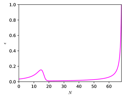
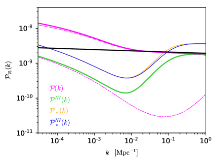
Figure 1: Left: Evolution of the slow-roll parameter $\epsilon$ for the double inflation model in Eq. (3.1) with $\chi_{0}=6m_{\phi}$. Right: The green line represents the scalar power spectrum found in Ref. [75] where the effect of isocurvature perturbation was neglected. See the magenta solid line for the correct result. In more detail, the magenta dashed (dotted) line shows the scalar power spectrum for $\mathcal{R}_{1}$ ($\mathcal{R}_{2}$). We also plot the power spectra at Hubble crossing computed taking (not taking) into account isocurvature perturbations in orange (blue) lines.

The curvature power spectrum obtained in [75] is plotted in the right panel of Fig. 1 in green line. However this result is obtained by neglecting the coupling between $\mathcal{R}$ and $\mathcal{S}$ in Eq. (2.17a). Taking into account the full evolution equations for $\mathcal{R}$ leads instead to the magenta solid power spectrum in the left panel of Fig. 1, i.e. to a nearly scale-invariant power spectrum on small scales with a bump on large scales. We also plot the power spectra at Hubble crossing computed by taking (not taking) into account isocurvature perturbations in orange (blue) lines: as expected, they are nearly the same, as the isocurvature sourcing inside the Hubble radius is negligible. We also plot in the right panel of Fig. 1 the curvature spectra corresponding to the two $\mathcal{R}_{1}$ and $\mathcal{R}_{2}$, computed properly taking into account the isocurvature perturbations. As it is easy to see, in this case, the full power spectrum is almost given by $\mathcal{P}_{\mathcal{R}_{1}}$ only, as we will show also for the model in the next Section.

The importance of isocurvature perturbations in the context of features in the PPS generated by a sharp turn in field space is not only limited to the model in Eq. (3.1) but is more general. See for instance Ref. [82, 89] for the inclusion of isocurvature perturbations in Roulette Inflation [93].

4 Generating features in the primordial power spectrum by a coupling between kinetic terms

In this section, we introduce a model in which primordial features at large scales of the desired form are more easily produced. We assume that the non-canonical function $b(\phi)$ has the form $b(\phi)=b_{1}\phi$, where $b_{1}$ is a constant with dimensions $M^{-1}$. We will see that the above simple form for the function $b(\phi)$ can lead to several type of features which could be observationally relevant for CMB anisotropies. Note that with this choice, the field space has an hyperbolic structure with a constant and negative Ricci curvature $R=-2db/d\phi^{2}=-2b_{1}^{2}$.

Although the mechanism we present is quite general for those initial conditions in which inflation is first driven by a field $\phi$ with an effective mass which is larger than $\chi$, we consider the following potential:

$$V(\phi,\,\chi)=\frac{m^{2}_{\phi}}{2}\phi^{2}+V_{0}\frac{\chi^{2}}{\chi_{0}^{2}+\chi^{2}}\,.$$ (4.1)

We consider a KKLTI-like potential [94] instead of a simplest mass term for $\chi$ in order to have a tensor-to-scalar ratio compatible with the most recent constraints [1, 95].

In Fig. 2, we plot relevant background quantities for the illustrative case of $(m_{\phi}\,M_{\textup{pl}})^{2}/V_{0}=1.2$, $\chi_{0}=0.06M_{\textup{pl}}$. We vary $b_{1}$ in order to highlight the effects of the coupling with the $\chi$ kinetic term. We choose $\phi_{i}=16\,M_{\textup{pl}}$ and $\chi_{i}=0.96\,M_{\textup{pl}}$ for the initial values of the scalar fields and we fix their initial time derivatives by imposing slow-roll initial conditions on $\dot{\phi}_{i}$ and $\dot{\chi}_{i}$. Note that this is not strictly necessary as the fields relax to the slow-roll attractors even if the velocities are chosen randomly. We consider sets of parameters that are relevant for observations in the next section.

As can be easily seen from Fig. 2, the heavier of the two fields, i.e. $\phi$, rolls down its potential driving a first phase of inflation while the lighter field $\chi$ remains frozen (see Ref. [96] for a detailed analytical description of the background evolution). This dynamics, also typical of multifield $\alpha$-attractor models [97, 98], can be easily understood as follows. For $b_{1}>0$ and the initial values of $\phi$ considered in Fig. 2, the term $\exp(2b(\phi))V_{\chi}$ can be safely taken as zero as a good approximation and a solution of Eq. (2.3b) is $\chi_{1}=\chi_{i}$, where the subscript $1$ is to specify that this solution is valid during the first stage of slow-roll. Therefore, the term proportional to $\dot{\chi}^{2}$ in Eq. (2.3a), along with $\ddot{\phi}$, can be discarded and the slow-roll solution to Eq. (2.3a) becomes simply:

$$\phi_{1}(N)=\sqrt{\phi_{i}^{2}+4M_{\textup{pl}}^{2}N}.$$ (4.2)

The first stage of inflation dominated by $\phi$ eventually ends and, after a few damped oscillations, the pattern of which depends on the potential ratio $(m_{\phi}\,M_{\textup{pl}})^{2}/V_{0}$, see also Appendix A, it settles to the effective minimum of its potential which is found by solving

$$V_{\phi}=b_{\phi}e^{2b}\dot{\chi}^{2}\simeq b_{\phi}\frac{e^{-2b}}{3}\left(\frac{V_{\chi}}{V(0,\,\chi)}\right)^{2},$$ (4.3)

which has a solution

$$\phi_{\textup{min}}\simeq\textup{const}\simeq\frac{\mathcal{W}\left(\frac{8b_{1}^{2}\chi_{0}^{4}}{3\chi_{i}^{6}}\right)}{2b_{1}}$$ (4.4)

where $\mathcal{W}$ is the D’Alambert W function and we have assumed $\chi\sim\chi_{i}$. The field $\chi$ then starts a second inflationary phase. The Klein-Gordon equation (2.3b) can be easily integrated to get

$$\chi_{2}(N)=\sqrt{-\chi_{0}^{2}+\sqrt{-8(N-N_{1})\chi_{0}^{2}+\left(\chi_{i}^{2}+\chi_{0}^{2}\right)^{2}}}e^{-2b_{1}\phi_{\textup{min}}},$$ (4.5)

where we have denoted by $N_{1}$ the beginning of the second stage of inflation. With this choice of parameters, although $\phi_{\textup{min}}$ is small, the non-canonical kinetic term affects the background dynamics in making the second inflationary phase longer, as the third term in Eq. (2.3b) acts as a friction term for the $\chi$ field exponentially, and to suppress $V_{\chi}$. As can be seen from the central panels of Fig. 2, the first slow-roll parameter $\epsilon$ shows a bump between the two phases and the slow-roll conditions are violated, i.e. $\epsilon_{2}\equiv\eta>1$.

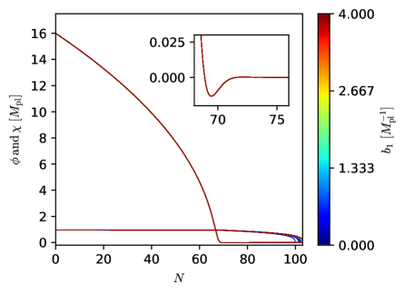
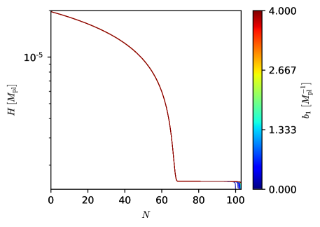
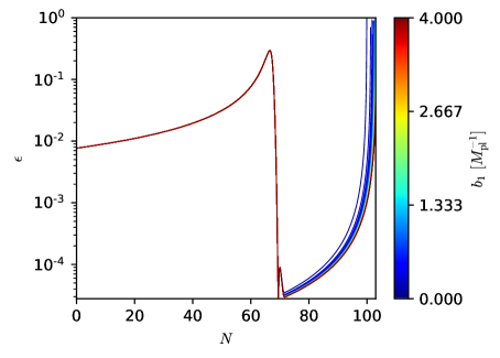
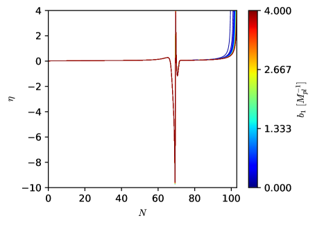
Figure 2: [Top] Evolution of the scalar fields (left) and the Hubble parameter $H$ (right). [Bottom] Evolution of the first two slow-roll parameters $\epsilon$ (left) and $\epsilon_{2}\equiv\eta$ (right). The ratio $(m_{\phi}\,M_{\textup{pl}})^{2}/V_{0}=1.2$ is fixed and $b_{1}$ is varied for a continuous range of values.

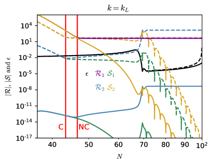
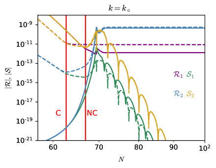
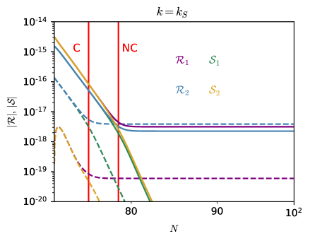
Figure 3: Evolution of the perturbed modes for a canonical coupling between the two scalar fields ($b_{1}=0$, dashed lines) and a non-canonical coupling with $b_{1}=4/M_{\mathrm{p}l}$ (continuous lines). We plot the evolution for the modes with $k_{L}/k_{\circ}\equiv 10^{-7}$ [Left], $k_{\circ}$ [Center] and $k_{S}/k_{\circ}\equiv 10^{5}$ [Right]. The red vertical lines signal the $e$-folds when the modes cross the Hubble radius. We also plot the $\epsilon$ parameter in black lines. The ratio $(m_{\phi}\,M_{\textup{pl}})^{2}/V_{0}=1.2$ is fixed.

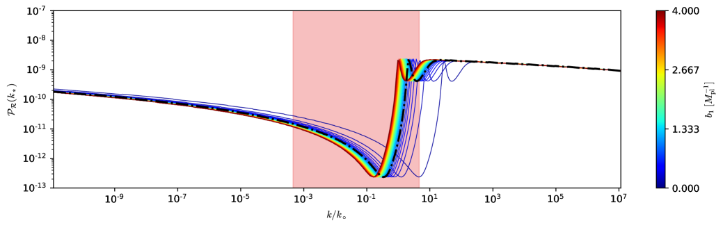
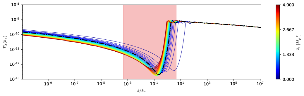
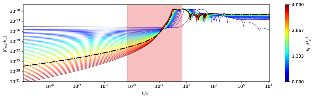
Figure 4: [Top] Curvature , [center] isocurvature, [bottom] curvature-isocurvature cross-correlation power spectra at Hubble crossing. The ratio $(m_{\phi}\,M_{\textup{pl}})^{2}/V_{0}=1.2$ is fixed and $b_{1}$ is varied for a continuous range of values. The $x$-axis is normalized to $k_{\circ}$, i.e. the scale which crosses the Hubble radius when $\epsilon$ reaches is maximum value in the dotted black model. The red band represent the range of scales that cross the Hubble radius during the range of $e$-folds when slow-roll is violated.

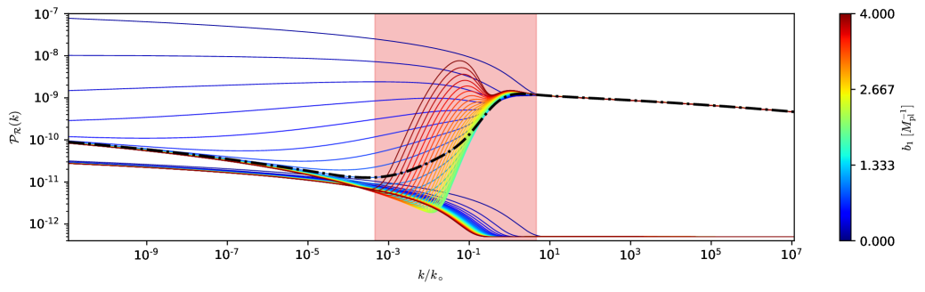
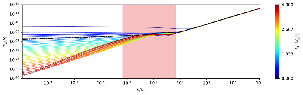
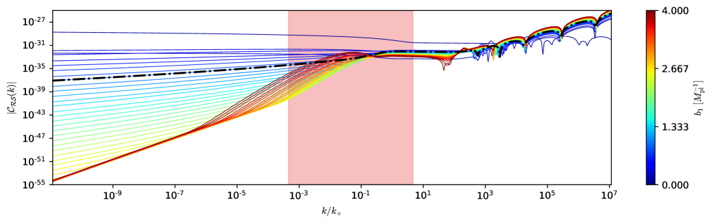
Figure 5: [Top] Curvature , [center] isocurvature, [bottom] curvature-isocurvature cross-correlation power spectra evaluated at the end of inflation. The ratio $(m_{\phi}\,M_{\textup{pl}})^{2}/V_{0}=1.2$ is fixed and $b_{1}$ is varied over a continuous range of values. In the top panel we also plot the tensor power spectrum evaluated at the end of inflation.

The evolution of fluctuations is shown in Fig. 5 for three different modes that cross the Hubble radius well before ($k=k_{L}$, large scale mode), at ($k=k_{\circ}$, transition mode) and after ($k=k_{S}$, small scales modes) the transition between the two stages of inflation. Solid (dashed) lines represent modes for $b_{1}=4/M_{\mathrm{pl}}$ ($b_{1}=0$). As can be seen, isocurvature modes are strongly suppressed by $b_{1}\neq 0$ in the super-Hubble regime compared to the case of standard kinetic terms: this effect is due to an effective mass for isocurvature perturbations which is larger than $H$ during the slow-roll regime. In the case of $k\sim k_{\circ}$, isocurvature perturbations grow for $b_{1}=4/M_{\mathrm{pl}}$ and source in turn curvature ones. This effect is due to the fact that for high values of $b_{1}$, the effective mass-squared for isocurvature perturbations becomes temporarily negative during slow-roll violation, leading to a tachyonic growth of isocurvature.

We now turn to the primordial power spectra. Features in the power spectrum can be generated at the scales that cross the Hubble radius around the transition between the first and the second stage of inflation and depend on the combination of both $b_{1}$ and the ratio of the potentials $(m_{\phi}\,M_{\textup{pl}})^{2}/V_{0}$. These are shown in Figs. 4 and 5, where we plot the curvature, isocurvature and curvature-isocurvature cross-correlation power spectra at Hubble crossing and at the end of inflation, respectively, for the same parameters used in Fig. 2.

We plot a broad range of wavenumbers on the $x$-axis in units of $k_{\circ}$, that we define as the scale that crosses the Hubble radius when slow-roll is violated in the black dashed model fixed by $b_{1}=2.4/M_{\textup{pl}}$, i.e. at the peak of $\epsilon$ in the black dotted line of Fig. 2. The red band is the range of scales that cross the Hubble radius during the break down of the slow-roll approximation. The part of the power spectrum that can be constrained by CMB observations consists of about $4$ e-folds and depends on the position of $k_{\circ}$ which, once fixed $N_{*}$, depends only on $\chi_{i}$.

As can be easily seen, apart from a small shift in the $k$-axis due to the different $k_{\circ}$, the power spectrum of curvature and isocurvature perturbations at the Hubble crossing is nearly the same for every value of $b_{1}$, as expected. The difference between curvature and isocurvature power spectra, however, is mainly due to the super-Hubble evolution of curvature and isocurvature perturbations, that we discuss in the following.

Below we provide the features appearing at different cosmological scales:

• Large scales:

  We first look at the largest scales in Figs. 4 and 5. If we decrease $\chi_{i}$ enough, slow-roll breaks down closer to the end of inflation and $k_{\circ}$ is shifted to the left of the plot. The power spectrum at CMB scales is then characterized by the spectral index predicted by chaotic inflation at the Hubble crossing. Note, however, that the amplitude of the scalar power spectrum depends on the non-canonical kinetic term $b_{1}$ because of the different isocurvature sourcing to $\mathcal{R}$.

  The tensor power spectrum, as expected, is not affected by any sources as it is decoupled from the scalar perturbations at first order. This in turn leads to a lower tensor to scalar ratio as discussed above. We will discuss a specific example of this in the next section.

• Small scales:

  At smaller scales, we have the inflationary predictions of the single-field inflation driven by the field $\chi_{i}$, i.e. KKLT inflation at Hubble crossing. We have a small change in the curvature power spectrum at the end of inflation since its change induced by isocurvature perturbations is small. Isocurvature perturbations are indeed suppressed when their wavenumber exceed the Hubble radius and therefore acquire a blue spectrum in this region. All the spectra have a negligible dependence on $b_{1}$ in this region.

  The reason is that the field $\phi$ has already settled in the minimum of its potential $\phi_{\textup{min}}\simeq 0$ and thus the effects of $b(\phi_{\textup{min}})\simeq 0$ are not as pronounced as in the first case.

  The power spectrum of isocurvature perturbations in Fig. 5 is indeed nearly the same for all the values of $b_{1}$ shown in the color-bar.

• Intermediate scales:

  This is the region where features are generated. The wavenumbers in this region cross the Hubble radius during the transition between the first and the second stage of inflation.

  As can be seen, since the larger and the smaller scales have different amplitudes, the power spectrum has a sudden rise to match the two amplitudes. If $k_{\circ}\simeq 10^{-3}\,\textup{Mpc}^{-1}$ and the plateau on the right side is properly normalized to the CMB normalization, then the junction between the two plateaus becomes a point of suppression of power at large scales. As we discuss in the next Section, this can be used to explain the low-$\ell$ deficit at $\ell\lesssim 40$ in the CMB temperature anisotropy pattern.

  Furthermore, as we increase $b_{1}$, a bump, followed by a small, dip appears. This is easily explained by looking at the inset in top left panel of Fig. 2, which contains an inset highlighting the evolution of the field $\phi$ near the transition. The field undergoes a damped oscillation around its minimum before settling in it. When $\phi$ decreases and eventually becomes negative, also $b(\phi)$ becomes negative and, if $b_{1}$ is large enough, the effective mass of isocurvature perturbations becomes negative as well for a few $e$-folds, leading to a brief instability for those modes that cross the Hubble radius around the violation of slow-roll. This results in an enhanced isocurvature feedback for the modes that cross the Hubble radius when $b(\phi)<0$. This effect is stronger for larger $b_{1}$ and the resulting bump might worsen the fit to CMB anisotropies. However, arbitrarily increasing $b_{1}$ would further increase the bump: this mechanism might be used to generate Primordial Black Holes (PBH) and a stochastic background of Gravitational Waves (GW) from second order effects, if $k_{\circ}$ is pushed towards smaller scales. This scenario is analyzed in Ref. [96].

In the upper panel of Fig. 5 we also illustrate the power spectrum of tensor modes. In this model, tensor modes are characterized by a larger amplitude for the modes which cross the Hubble radius during the first phase of inflation driven by a quadratic potential. The second phase of inflation is characterized by a tensor-to-scalar ratio typical of a KKLTI potential. This sort of broken power-law spectrum for tensor modes with a larger amplitude at large wavelengths might be therefore an interesting target for the next generation space missions dedicated to CMB polarization measurements as discussed in the next section.

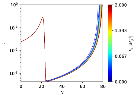
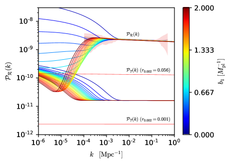
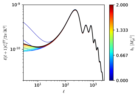
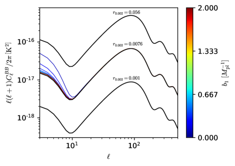
Figure 6: [Top-left] $\epsilon$ parameter for a continuous range of values of $b_{1}$. [Top-right] curvature and tensor power spectra together with the $1$ and $2\sigma$ contours of the reconstructed primordial power spectrum by Planck [1], the upper bound on the tensor power spectrum (purple line) inferred by the combined analysis of Planck, BAO, BICEP2, and Keck Array [95] and the $r_{0.002}=0.001$ target of future CMB experiments [100, 101, 102, 103]. [Bottom-left] predictions on the CMB temperature lensed angular spectra. The black solid line is the Planck best-fit obtained with $r_{0.002}=0.056$. [Bottom-right] primordial B-mode angular spectra together with the ones computed with the consistency relation $r=-8n_{T}$ for $r_{0.002}=0.0056,\,0.0208,\,\text{and}\,0.001$ in black solid lines. The parameters used in the plot are $(m_{\phi}\,M_{\textup{pl}})^{2}/V_{0}=1.07624$, $\chi_{0}=\sqrt{3}M_{\textup{pl}}$ $\phi_{i}=8.8\,M_{\textup{pl}}$ and $\chi_{i}=5.76\,M_{\textup{pl}}$.

5 Effects on the CMB anisotropy power spectra

We now show the importance of the non-canonical coupling in generating primordial features which could be connected to the deficit at large scales in the CMB temperature anisotropy power spectrum. In order to achieve a deficit at $\ell\lesssim 40$, we shift the $k_{\circ}$ in Fig. 5 around $k_{\circ}\sim 10^{-3}\,\textup{Mpc}^{-1}$. To do so, we need the second stage of inflation to last about $46-47$ $e$-folds (we remind that we fix $N_{*}=50$ in our analysis). This is achieved, by setting $\chi_{i}=5.76M_{\textup{pl}}$. The evolution of $\epsilon$ for this model is given in the top left panel of Fig. 6, where we have also listed all the parameters used in the numerical integration, that we have performed using a modified version of the publicly available code BINGO [104], that takes into account the full two fields dynamics. Note that the amplitude of the tensor power spectrum is larger than in Fig. 5, as we have used $\chi_{0}=\sqrt{3}\,M_{\textup{pl}}$, differently from Sec. 4.

In the top right panel, we plot the results for the curvature and tensor power spectra. We obtain a suppression of power on large scales starting from $0.7M_{\mathrm{pl}}^{-1}\lesssim b_{1}\lesssim 2M_{\mathrm{pl}}^{-1}$. The tensor power spectrum shows a larger amplitude at low $k$, as also shown in Fig. 5, because the Hubble parameter $H$ is larger during the first stage of inflation.

The corresponding imprints on the CMB angular power spectra, that we computed using the Einstein-Boltzmann code CLASS [105], are shown in the lower panels of Fig. 6. There is a lack of power in the CMB temperature power spectrum at low multipoles, without any modification to its small scale peak structure , more similar to what happens in Punctuated Inflation [25] rather than for a discontinuity in the first derivative of the inflaton potential [77]. This mechanism can be therefore interesting to explain the low-$\ell$ deficit in the CMB temperature power spectrum in both the WMAP and Planck data [106, 95] and is different from other ones such as Punctuated Inflation [25] or a discontinuity in the first derivative of the inflaton potential [77]. For the same parameters, the larger amplitude in the tensor power spectrum at low $k$ induce a larger primordial B-mode polarization signal with respect to the single field realization of the second inflationary phase at $\ell\lesssim 30$, where the reionization bump is located. Again, this prediction for B-modes would be different from the corresponding one in presence of a discontinuity in the first derivative of the inflaton potential [77]. We note, however, that in the model considered, all the larger primordial B-mode occur for values of $b_{1}$ that give a higher contribution to the larger scale temperature spectra as well.

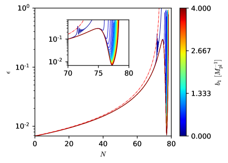
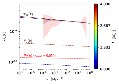
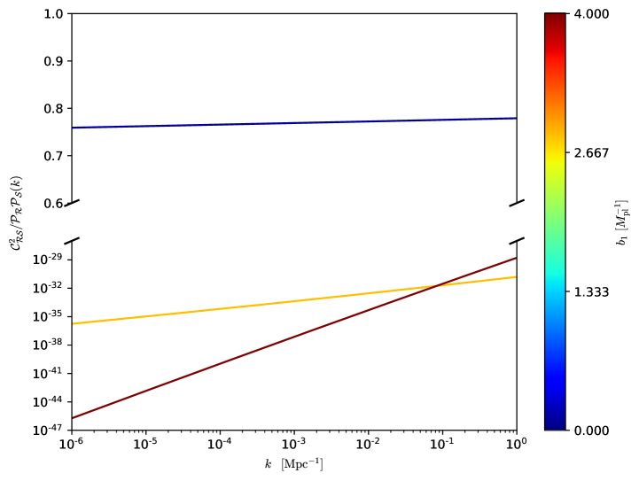
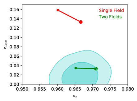
Figure 7: [Top-left] $\epsilon$ parameter. The red dashed line is the single-field version with the same $\phi_{i}$ and without the field $\chi$. [Top-right] curvature (solid), tensor (dashed) and isocurvature (dotted) power spectra for three models with $b_{1}=0,\,2.8,\,4.0$ (see color-bar) together with the upper bound on the tensor power spectrum (red line) inferred by the combined analysis of Planck and BICEP-Keck Array and the $1$ and $2\sigma$ contours of the reconstructed primordial power spectrum by Planck [1]. Note that the ratio between the potential has been adjusted to match the amplitude $A_{s}$ of $\mathcal{P}_{\mathcal{R}}$. [Bottom-left] Curvature and isocurvature cross-correlation normalized to the curvature and isocurvature spectra. [Bottom-right] predictions in the $n_{s}-r$ plane of the chaotic single-field model (red) and our model with $b_{1}=0$ (green) on top of the $1$ and $2\sigma$ contours by Planck. Small (large) circles denote $N_{*}=50\,(60)$. for a continuous range of values of $b_{1}$. The parameters used in the plot are $(m_{\phi}\,M_{\textup{pl}})^{2}/V_{0}=1.17855$, $\phi_{i}=17\,M_{\textup{pl}}$ and $\chi_{i}=0.42\,$ and in the three plots $b_{1}$ is varied for a continuous range of values.

Let us now discuss the case in which the transition between the two stages occurs closer to the end of inflation, as shown in Fig. 7. Whereas some differences in the scalar power spectrum and scalar tilt are present with respect to a single field realization of the first inflationary stage, i.e. a quadratic potential [107], the tensor-to-scalar ratio can be suppressed by the correlation between curvature and isocurvature perturbations. The small differences in the scalar power spectra are due to the longer duration of inflation because of the second stage, as can be seen from the insert in top left panel of Fig. 7. Fig. 7 also shows that, for the particular model in Eq. (4.1), the prediction for $r$ in the first inflationary phase driven by a quadratic potential can be reconciled with the most recent constraints by CMB anisotropies since cross-correlation between isocurvature and curvature perturbation can modify the relation between the tensor-to-scalar ratio and the tensor tilt [108, 109, 81, 110, 111, 112, 113]

$$r=-n_{T}\left(1-\frac{\mathcal{C}_{\mathcal{R}\mathcal{S}}^{2}}{\mathcal{P}_{\mathcal{R}}\mathcal{P}_{\mathcal{S}}}\right).$$ (5.1)

As can be seen from the bottom left panel in Fig. 7, the cross-correlation is indeed larger when $b_{1}=0$, thus explaining the lower tensor-to-scalar ratio. We note that we have checked that $\mathcal{P}_{\mathcal{S}}$ is small for all the models in Fig. 7.

Note that the mechanism just presented differs from earlier attempts to cure single field models that are in tension with the Planck data with the addition of heavy [114, 115] and/or spectator fields during inflation [116, 117, 118, 119, 120, 121]. In fact, it is the presence of a second, lighter inflaton that modifies the single-field predictions in our model.

6 Discussions and conclusions

Generating features at large scales in single-field inflationary models requires in general either a fine-tuned scalar field Lagrangian or exotic initial conditions in the background dynamics/quantum fluctuations. On the other hand, generating features of similar shape by turning trajectories in field space in multi-field inflationary models requires also a careful study of isocurvature modes and their effects on the curvature perturbations. Isocurvature perturbations can indeed erase features in the PPS generated at Hubble crossing, as we have explicitly shown for the archetypal case of inflation driven by two massive scalar fields [91], leading to different conclusions from [75]. Isocurvature fluctuations can have an impact on other inspired multi-field models for primordial features as well.

We have then discussed the phenomenology of features at large scales in two field inflationary models in which there is a non-trivial kinetic term of a second field $\chi$ coupled to $\phi$. We have restricted ourselves to the case of a separable potential in which features can be generated during a breakdown of the slow-roll regime between two phases of inflation driven first by a scalar field with a larger effective mass and then by a second field with a smaller one. We have numerically integrated the exact equations for the linear perturbations taking into account the super-Hubble evolution of curvature and isocurvature perturbations.

We have shown how a sufficiently large coupling ($b\gtrsim M^{-1}_{\mathrm{pl}}$) with the kinetic term of the second field can lead to a suppression of isocurvature perturbations, therefore decreasing their feedback into curvature perturbations. We have computed the associated CMB power spectra showing the phenomenological relevance of this mechanism to produce the low-$\ell$ deficit observed in the temperature power spectrum. For the same parameters, we have also shown how the tensor power spectrum can have a larger amplitude at small $k$ since the Hubble parameter is larger in the first inflationary phase. For this last reason, the mechanism discussed here is potentially different from other single field inflationary models which produce a deficit in the CMB temperature power spectrum at low multipoles, without decreasing the B-mode polarization signal as for a short inflationary stage preceeded by a kinetic stage [21, 122]. This possibility is obviously of interest for the next generation experiments dedicated to CMB polarization which can have access to low multipoles [100, 101, 102].

On the other hand, we have also shown that, when the breakdown of slow-roll occurs close to the end of inflation, isocurvature perturbations can enhance the scalar PPS without altering the tensor one if the two fields are canonically coupled, and therefore reducing the tensor-to-scalar ratio on CMB scales.

In terms of future work, we note that the breakdown of the slow-roll regime would probably lead to a certain level of non-Gaussianity. We hope to study this issue in the future.

Appendix A Varying the ratio of the potentials

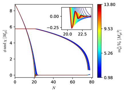
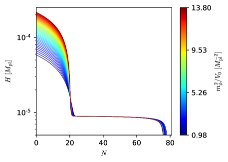
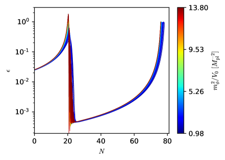
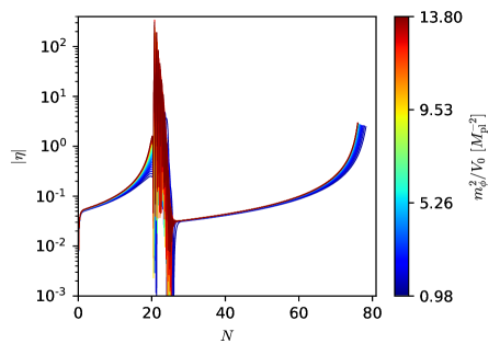
Figure 8: [Top-left] Scalar fields and [top-right] Hubble parameter $H$ evolution. [Bottom-left] First slow-roll parameter $\epsilon$ and [top-right] second slow-roll parameter $\eta\equiv\epsilon_{2}$. The non-canonical coupling $b_{1}=1/M_{\textup{pl}}$ is fixed and we vary the potential ratio $(m_{\phi}\,M_{\textup{pl}})^{2}/V_{0}$ for a continuous range of values.

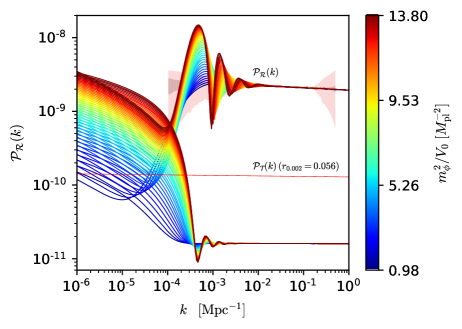
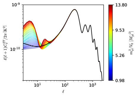
Figure 9: [Left] scalar and tensor power spectrum for the model Eq. (4.1). [Right] predictions on the CMB temperature lensed angular spectra. The red dashed line denotes the Planck 18 + BK15 95 % CL upper bound on $r$, i.e. $r_{0.002}=0.056$. The non-canonical coupling $b_{1}=1/M_{\textup{pl}}$ is fixed and we vary the potential ratio $(m_{\phi}\,M_{\textup{pl}})^{2}/V_{0}$ for a continuous range of values.

In the main text, we have shown the effects of the non-canonical kinetic coupling of the two scalar fields. In particular, we have observed that, at a fixed potential ratio, higher values of the coupling $b_{1}$ can either enhance or suppress isocurvature perturbations and their feedback into the scalar PPS, depending on the sign of the scalar field $\phi$. The goal of this Appendix is to provide a full scan of the parameter space of our toy model, showing the effect of varying the potential ratio $(m_{\phi}\,M_{\textup{pl}})^{2}/V_{0}$.

The background evolution of the model is shown in Fig. 8. As can be seen, by increasing the ratio of the potentials, the energy scale of the first inflationary stage becomes higher and the transition between the two stages more violent. This results in a huge deviation from $\eta\simeq\mathcal{O}(1)$ of the second slow-roll parameter. Also, the first slow-roll parameter can become even greater than unity, leading to an intermediate matter-dominated expansion [74]. During this transition, the heavier scalar field undergoes damped oscillations around its minimum. These can last up to $\sim 5$ $e$-folds as can be seen from the inset in the top left panel of Fig. 8.

Following the reasoning of Section 4, the damped oscillations between positive and negative values of the field $\phi$ leads to a continuous suppression and increase of isocurvature sourcing to the curvature perturbation. This series of peaks and dips can be thus seen in the power spectrum at scales that leave the horizon during this background oscillatory phase. This is shown in the left panel of Fig. 9, where we plot the scalar and tensor power spectrum for our model obtained by fixing $b_{1}$ and varying the potential ratio. As can be seen, the oscillating pattern of the field $\phi$ is indeed imprinted in both the scalar and tensor power spectra.

Nevertheless, the damped oscillations have a high amplitude at large scales. The oscillations have therefore to be at unobservable scales to fit the CMB data. In this case the CMB angular power spectra are in fact very similar to those obtained using a power-law power spectrum. On the other hand, if the oscillations in the power spectrum are in the range $10^{-4}-10^{-2}$ $\text{Mpc}^{-1}$ as in the left panel of Fig. 9, we obtain the CMB angular power spectra in the right panel of Fig. 9. As can be seen, the range of multipoles $\ell\leq 100$ is totally different from the $\Lambda$CDM best-fit plotted in solid black lines and the fit to data is considerably affected.

References

- [1] Planck collaboration, Y. Akrami et al., Planck 2018 results. X. Constraints on inflation, 1807.06211.
- [2] Planck collaboration, Y. Akrami et al., Planck 2018 results. IX. Constraints on primordial non-Gaussianity, 1905.05697.
- [3] S. Hannestad, Reconstructing the inflationary power spectrum from cosmic microwave background radiation data, Physical Review D 63 (2001) .
- [4] M. Tegmark and M. Zaldarriaga, Separating the early universe from the late universe: Cosmological parameter estimation beyond the black box, Physical Review D 66 (2002) .
- [5] P. Mukherjee and Y. Wang, Model‐independent reconstruction of the primordial power spectrum fromwilkinson microwave anistropy probedata, The Astrophysical Journal 599 (2003) 1.
- [6] D. Tocchini-Valentini, Y. Hoffman and J. Silk, Non-parametric reconstruction of the primordial power spectrum at horizon scales from wmap data, Mon. Not. Roy. Astron. Soc. 367 (2006) 1095 [astro-ph/0509478].
- [7] A. Shafieloo and T. Souradeep, Primordial power spectrum from wmap, Physical Review D 70 (2004) .
- [8] N. Kogo, M. Sasaki and J. Yokoyama, Constraining cosmological parameters by the cosmic inversion method, Progress of Theoretical Physics 114 (2005) 555.
- [9] S. M. Leach, Measuring the primordial power spectrum: Principal component analysis of the cosmic microwave background, Mon. Not. Roy. Astron. Soc. 372 (2006) 646 [astro-ph/0506390].
- [10] A. Shafieloo and T. Souradeep, Estimation of primordial spectrum with post-wmap 3-year data, Physical Review D 78 (2008) .
- [11] P. Paykari and A. H. Jaffe, Optimal binning of the primordial power spectrum, The Astrophysical Journal 711 (2010) 1.
- [12] G. Nicholson and C. R. Contaldi, Reconstruction of the Primordial Power Spectrum using Temperature and Polarisation Data from Multiple Experiments, JCAP 07 (2009) 011 [0903.1106].
- [13] C. Gauthier and M. Bucher, Reconstructing the primordial power spectrum from the cmb, Journal of Cosmology and Astroparticle Physics 2012 (2012) 050.
- [14] R. Hlozek, J. Dunkley, G. Addison, J. W. Appel, J. R. Bond, C. S. Carvalho et al., The atacama cosmology telescope: A measurement of the primordial power spectrum, The Astrophysical Journal 749 (2012) 90.
- [15] J. A. Vázquez, M. Bridges, M. Hobson and A. Lasenby, Model selection applied to reconstruction of the primordial power spectrum, Journal of Cosmology and Astroparticle Physics 2012 (2012) 006.
- [16] D. K. Hazra, A. Shafieloo and T. Souradeep, Primordial power spectrum: a complete analysis with the wmap nine-year data, Journal of Cosmology and Astroparticle Physics 2013 (2013) 031.
- [17] P. Hunt and S. Sarkar, Reconstruction of the primordial power spectrum of curvature perturbations using multiple data sets, Journal of Cosmology and Astroparticle Physics 2014 (2014) 025.
- [18] D. K. Hazra, A. Shafieloo and T. Souradeep, Primordial power spectrum from Planck, JCAP 1411 (2014) 011 [1406.4827].
- [19] G. Brando and E. V. Linder, Exploring Early and Late Cosmology with Next Generation Surveys, 2001.07738.
- [20] A. A. Starobinsky, Spectrum of adiabatic perturbations in the universe when there are singularities in the inflation potential, JETP Lett. 55 (1992) 489.
- [21] C. R. Contaldi, M. Peloso, L. Kofman and A. D. Linde, Suppressing the lower multipoles in the CMB anisotropies, JCAP 0307 (2003) 002 [astro-ph/0303636].
- [22] L. Sriramkumar and T. Padmanabhan, Initial state of matter fields and trans-Planckian physics: Can CMB observations disentangle the two?, Phys. Rev. D71 (2005) 103512 [gr-qc/0408034].
- [23] R. Allahverdi and A. Mazumdar, Spectral tilt in A-term inflation, arXiv e-prints (2006) hep [hep-ph/0610069].
- [24] R. K. Jain, P. Chingangbam and L. Sriramkumar, On the evolution of tachyonic perturbations at super-Hubble scales, JCAP 10 (2007) 003 [astro-ph/0703762].
- [25] R. K. Jain, P. Chingangbam, J.-O. Gong, L. Sriramkumar and T. Souradeep, Punctuated inflation and the low CMB multipoles, JCAP 0901 (2009) 009 [0809.3915].
- [26] R. K. Jain, P. Chingangbam, L. Sriramkumar and T. Souradeep, The tensor-to-scalar ratio in punctuated inflation, Phys. Rev. D 82 (2010) 023509 [0904.2518].
- [27] E. Ramirez and D. J. Schwarz, Predictions of just-enough inflation, Phys. Rev. D 85 (2012) 103516 [1111.7131].
- [28] E. Ramirez, Low power on large scales in just enough inflation models, Phys. Rev. D 85 (2012) 103517 [1202.0698].
- [29] D. K. Hazra, A. Shafieloo, G. F. Smoot and A. A. Starobinsky, Wiggly Whipped Inflation, JCAP 08 (2014) 048 [1405.2012].
- [30] D. K. Hazra, A. Shafieloo, G. F. Smoot and A. A. Starobinsky, Inflation with Whip-Shaped Suppressed Scalar Power Spectra, Physical Review Letters 113 (2014) 071301 [1404.0360].
- [31] R. Bousso, D. Harlow and L. Senatore, Inflation After False Vacuum Decay: New Evidence from BICEP2, JCAP 1412 (2014) 019 [1404.2278].
- [32] D. K. Hazra, A. Shafieloo, G. F. Smoot and A. A. Starobinsky, Primordial features and Planck polarization, JCAP 1609 (2016) 009 [1605.02106].
- [33] A. Gruppuso, N. Kitazawa, N. Mandolesi, P. Natoli and A. Sagnotti, Pre-Inflationary Relics in the CMB?, Phys. Dark Univ. 11 (2016) 68 [1508.00411].
- [34] D. K. Hazra, D. Paoletti, M. Ballardini, F. Finelli, A. Shafieloo, G. F. Smoot et al., Probing features in inflaton potential and reionization history with future CMB space observations, JCAP 1802 (2018) 017 [1710.01205].
- [35] L. Hergt, W. Handley, M. Hobson and A. Lasenby, Constraining the kinetically dominated Universe, Phys. Rev. D 100 (2019) 023501 [1809.07737].
- [36] M. Ballardini, Probing primordial features with the primary CMB, Phys. Dark Univ. 23 (2019) 100245 [1807.05521].
- [37] H. Ragavendra, D. Chowdhury and L. Sriramkumar, Unique contributions to the scalar bispectrum in ‘just enough inflation’, 1906.03942.
- [38] H. Ragavendra, D. Chowdhury and L. Sriramkumar, Suppression of scalar power on large scales and associated bispectra, 2003.01099.
- [39] J. A. Adams, B. Cresswell and R. Easther, Inflationary perturbations from a potential with a step, Phys. Rev. D64 (2001) 123514 [astro-ph/0102236].
- [40] X. Chen, R. Easther and E. A. Lim, Large Non-Gaussianities in Single Field Inflation, JCAP 06 (2007) 023 [astro-ph/0611645].
- [41] L. Covi, J. Hamann, A. Melchiorri, A. Slosar and I. Sorbera, Inflation and WMAP three year data: Features have a Future!, Phys. Rev. D74 (2006) 083509 [astro-ph/0606452].
- [42] D. K. Hazra, M. Aich, R. K. Jain, L. Sriramkumar and T. Souradeep, Primordial features due to a step in the inflaton potential, JCAP 1010 (2010) 008 [1005.2175].
- [43] V. Miranda, W. Hu and P. Adshead, Warp Features in DBI Inflation, Phys. Rev. D86 (2012) 063529 [1207.2186].
- [44] M. Benetti, Updating constraints on inflationary features in the primordial power spectrum with the Planck data, Phys. Rev. D88 (2013) 087302 [1308.6406].
- [45] A. Gallego Cadavid and A. E. Romano, Effects of discontinuities of the derivatives of the inflaton potential, Eur. Phys. J. C75 (2015) 589 [1404.2985].
- [46] J. Chluba, J. Hamann and S. P. Patil, Features and New Physical Scales in Primordial Observables: Theory and Observation, Int. J. Mod. Phys. D24 (2015) 1530023 [1505.01834].
- [47] M. Ballardini, F. Finelli, R. Maartens and L. Moscardini, Probing primordial features with next-generation photometric and radio surveys, JCAP 1804 (2018) 044 [1712.07425].
- [48] J. Martin and C. Ringeval, Superimposed oscillations in the WMAP data?, Phys. Rev. D69 (2004) 083515 [astro-ph/0310382].
- [49] A. Ashoorioon and A. Krause, Power Spectrum and Signatures for Cascade Inflation, hep-th/0607001.
- [50] X. Chen, R. Easther and E. A. Lim, Generation and Characterization of Large Non-Gaussianities in Single Field Inflation, JCAP 04 (2008) 010 [0801.3295].
- [51] T. Biswas, A. Mazumdar and A. Shafieloo, Wiggles in the cosmic microwave background radiation: echoes from non-singular cyclic-inflation, Phys. Rev. D82 (2010) 123517 [1003.3206].
- [52] R. Flauger, L. McAllister, E. Pajer, A. Westphal and G. Xu, Oscillations in the CMB from Axion Monodromy Inflation, JCAP 1006 (2010) 009 [0907.2916].
- [53] C. Pahud, M. Kamionkowski and A. R. Liddle, Oscillations in the inflaton potential?, Phys. Rev. D79 (2009) 083503 [0807.0322].
- [54] A. Achucarro, J.-O. Gong, S. Hardeman, G. A. Palma and S. P. Patil, Mass hierarchies and non-decoupling in multi-scalar field dynamics, Phys. Rev. D84 (2011) 043502 [1005.3848].
- [55] M. Aich, D. K. Hazra, L. Sriramkumar and T. Souradeep, Oscillations in the inflaton potential: Complete numerical treatment and comparison with the recent and forthcoming CMB datasets, Phys. Rev. D87 (2013) 083526 [1106.2798].
- [56] D. K. Hazra, Changes in the halo formation rates due to features in the primordial spectrum, JCAP 1303 (2013) 003 [1210.7170].
- [57] H. Peiris, R. Easther and R. Flauger, Constraining Monodromy Inflation, JCAP 1309 (2013) 018 [1303.2616].
- [58] P. D. Meerburg and D. N. Spergel, Searching for oscillations in the primordial power spectrum. II. Constraints from Planck data, Phys. Rev. D89 (2014) 063537 [1308.3705].
- [59] R. Easther and R. Flauger, Planck Constraints on Monodromy Inflation, JCAP 1402 (2014) 037 [1308.3736].
- [60] X. Chen, M. H. Namjoo and Y. Wang, Models of the Primordial Standard Clock, JCAP 1502 (2015) 027 [1411.2349].
- [61] H. Motohashi and W. Hu, Running from Features: Optimized Evaluation of Inflationary Power Spectra, Phys. Rev. D92 (2015) 043501 [1503.04810].
- [62] V. Miranda, W. Hu, C. He and H. Motohashi, Nonlinear Excitations in Inflationary Power Spectra, Phys. Rev. D93 (2016) 023504 [1510.07580].
- [63] M. Ballardini, F. Finelli, C. Fedeli and L. Moscardini, Probing primordial features with future galaxy surveys, JCAP 10 (2016) 041 [1606.03747].
- [64] M. Ballardini, R. Murgia, M. Baldi, F. Finelli and M. Viel, Non-linear damping of superimposed primordial oscillations on the matter power spectrum in galaxy surveys, 1912.12499.
- [65] D. Wands, Multiple field inflation, Lect. Notes Phys. 738 (2008) 275 [astro-ph/0702187].
- [66] L. A. Kofman and D. Yu. Pogosian, Nonflat Perturbations in Inflationary Cosmology, Phys. Lett. B214 (1988) 508.
- [67] L. C. Price, J. Frazer, J. Xu, H. V. Peiris and R. Easther, MultiModeCode: An efficient numerical solver for multifield inflation, JCAP 1503 (2015) 005 [1410.0685].
- [68] D. J. H. Chung, E. W. Kolb, A. Riotto and I. I. Tkachev, Probing Planckian physics: Resonant production of particles during inflation and features in the primordial power spectrum, Phys. Rev. D62 (2000) 043508 [hep-ph/9910437].
- [69] S. Pi, Y.-l. Zhang, Q.-G. Huang and M. Sasaki, Scalaron from -gravity as a heavy field, JCAP 1805 (2018) 042 [1712.09896].
- [70] T. Mori, K. Kohri and J. White, Multi-field effects in a simple extension of inflation, JCAP 1710 (2017) 044 [1705.05638].
- [71] A. Gundhi and C. F. Steinwachs, Scalaron-Higgs inflation, Nucl. Phys. B954 (2020) 114989 [1810.10546].
- [72] X. Gao, D. Langlois and S. Mizuno, Influence of heavy modes on perturbations in multiple field inflation, JCAP 1210 (2012) 040 [1205.5275].
- [73] A. Achucarro, J.-O. Gong, S. Hardeman, G. A. Palma and S. P. Patil, Features of heavy physics in the CMB power spectrum, JCAP 1101 (2011) 030 [1010.3693].
- [74] D. Polarski and A. A. Starobinsky, Spectra of perturbations produced by double inflation with an intermediate matter dominated stage, Nucl. Phys. B385 (1992) 623.
- [75] B. Feng and X. Zhang, Double inflation and the low cmb quadrupole, Phys. Lett. B570 (2003) 145 [astro-ph/0305020].
- [76] A. L. Berkin and K.-I. Maeda, Inflation in generalized Einstein theories, Phys. Rev. D44 (1991) 1691.
- [77] A. A. Starobinsky and J. Yokoyama, Density fluctuations in Brans-Dicke inflation, in Proceedings, Workshop on General Relativity and Gravitation (JGRG4): Kyoto, Japan, November 28-December 1, 1994, p. 381, 1994, gr-qc/9502002.
- [78] J. Garcia-Bellido and D. Wands, Constraints from inflation on scalar - tensor gravity theories, Phys. Rev. D52 (1995) 6739 [gr-qc/9506050].
- [79] A. A. Starobinsky, S. Tsujikawa and J. Yokoyama, Cosmological perturbations from multifield inflation in generalized Einstein theories, Nucl. Phys. B610 (2001) 383 [astro-ph/0107555].
- [80] F. Di Marco, F. Finelli and R. Brandenberger, Adiabatic and isocurvature perturbations for multifield generalized Einstein models, Phys. Rev. D67 (2003) 063512 [astro-ph/0211276].
- [81] F. Di Marco and F. Finelli, Slow-roll inflation for generalized two-field Lagrangians, Phys. Rev. D71 (2005) 123502 [astro-ph/0505198].
- [82] Z. Lalak, D. Langlois, S. Pokorski and K. Turzynski, Curvature and isocurvature perturbations in two-field inflation, JCAP 0707 (2007) 014 [0704.0212].
- [83] C. Gordon, D. Wands, B. A. Bassett and R. Maartens, Adiabatic and entropy perturbations from inflation, Phys. Rev. D63 (2001) 023506 [astro-ph/0009131].
- [84] S. Groot Nibbelink and B. J. W. van Tent, Scalar perturbations during multiple field slow-roll inflation, Class. Quant. Grav. 19 (2002) 613 [hep-ph/0107272].
- [85] D. J. Schwarz, C. A. Terrero-Escalante and A. A. Garcia, Higher order corrections to primordial spectra from cosmological inflation, Phys. Lett. B517 (2001) 243 [astro-ph/0106020].
- [86] V. F. Mukhanov, H. A. Feldman and R. H. Brandenberger, Theory of cosmological perturbations. Part 1. Classical perturbations. Part 2. Quantum theory of perturbations. Part 3. Extensions, Phys. Rept. 215 (1992) 203.
- [87] S. Cremonini, Z. Lalak and K. Turzynski, Strongly Coupled Perturbations in Two-Field Inflationary Models, JCAP 1103 (2011) 016 [1010.3021].
- [88] S. Tsujikawa, D. Parkinson and B. A. Bassett, Correlation - consistency cartography of the double inflation landscape, Phys. Rev. D67 (2003) 083516 [astro-ph/0210322].
- [89] C. van de Bruck and M. Robinson, Power Spectra beyond the Slow Roll Approximation in Theories with Non-Canonical Kinetic Terms, JCAP 1408 (2014) 024 [1404.7806].
- [90] J. Silk and M. S. Turner, Double Inflation, Phys. Rev. D35 (1987) 419.
- [91] D. Polarski and A. A. Starobinsky, Isocurvature perturbations in multiple inflationary models, Phys. Rev. D50 (1994) 6123 [astro-ph/9404061].
- [92] J. Lesgourgues and D. Polarski, CMB anisotropy predictions for a model of double inflation, Phys. Rev. D56 (1997) 6425 [astro-ph/9710083].
- [93] J. R. Bond, L. Kofman, S. Prokushkin and P. M. Vaudrevange, Roulette inflation with Kahler moduli and their axions, Phys. Rev. D75 (2007) 123511 [hep-th/0612197].
- [94] R. Kallosh, A. Linde and Y. Yamada, Planck 2018 and Brane Inflation Revisited, JHEP 01 (2019) 008 [1811.01023].
- [95] Planck collaboration, N. Aghanim et al., Planck 2018 results. VI. Cosmological parameters, 1807.06209.
- [96] M. Braglia, D. K. Hazra, F. Finelli, G. F. Smoot, L. Sriramkumar and A. A. Starobinsky, Generating PBHs and small-scale GWs in two-field models of inflation, JCAP 08 (2020) 001 [2005.02895].
- [97] A. Linde, D.-G. Wang, Y. Welling, Y. Yamada and A. Achúcarro, Hypernatural inflation, JCAP 07 (2018) 035 [1803.09911].
- [98] O. Iarygina, E. I. Sfakianakis, D.-G. Wang and A. Achucarro, Universality and scaling in multi-field -attractor preheating, JCAP 06 (2019) 027 [1810.02804].
- [99] S. Pi, M. Sasaki and Y.-l. Zhang, Primordial Tensor Perturbation in Double Inflationary Scenario with a Break, JCAP 06 (2019) 049 [1904.06304].
- [100] M. Hazumi et al., LiteBIRD: A Satellite for the Studies of B-Mode Polarization and Inflation from Cosmic Background Radiation Detection, J. Low. Temp. Phys. 194 (2019) 443.
- [101] CORE collaboration, J. Delabrouille et al., Exploring cosmic origins with CORE: Survey requirements and mission design, JCAP 1804 (2018) 014 [1706.04516].
- [102] M. Alvarez et al., PICO: Probe of Inflation and Cosmic Origins, 1908.07495.
- [103] NASA PICO collaboration, S. Hanany et al., PICO: Probe of Inflation and Cosmic Origins, 1902.10541.
- [104] D. K. Hazra, L. Sriramkumar and J. Martin, Bingo: a code for the efficient computation of the scalar bi-spectrum, Journal of Cosmology and Astroparticle Physics 2013 (2013) 026.
- [105] D. Blas, J. Lesgourgues and T. Tram, The Cosmic Linear Anisotropy Solving System (CLASS) II: Approximation schemes, JCAP 1107 (2011) 034 [1104.2933].
- [106] C. L. Bennett, D. Larson, J. L. Weiland, N. Jarosik, G. Hinshaw, N. Odegard et al., Nine-yearwilkinson microwave anisotropy probe(wmap) observations: Final maps and results, The Astrophysical Journal Supplement Series 208 (2013) 20.
- [107] A. D. Linde, Chaotic Inflation, Phys. Lett. 129B (1983) 177.
- [108] N. Bartolo, S. Matarrese and A. Riotto, Adiabatic and isocurvature perturbations from inflation: Power spectra and consistency relations, Phys. Rev. D64 (2001) 123504 [astro-ph/0107502].
- [109] D. Wands, N. Bartolo, S. Matarrese and A. Riotto, An Observational test of two-field inflation, Phys. Rev. D66 (2002) 043520 [astro-ph/0205253].
- [110] C. T. Byrnes and D. Wands, Curvature and isocurvature perturbations from two-field inflation in a slow-roll expansion, Phys. Rev. D74 (2006) 043529 [astro-ph/0605679].
- [111] S. Dimopoulos, S. Kachru, J. McGreevy and J. G. Wacker, N-flation, JCAP 0808 (2008) 003 [hep-th/0507205].
- [112] R. Easther, J. Frazer, H. V. Peiris and L. C. Price, Simple predictions from multifield inflationary models, Phys. Rev. Lett. 112 (2014) 161302 [1312.4035].
- [113] L. C. Price, H. V. Peiris, J. Frazer and R. Easther, Gravitational wave consistency relations for multifield inflation, Phys. Rev. Lett. 114 (2015) 031301 [1409.2498].
- [114] A. Achúcarro, V. Atal and Y. Welling, On the viability of and natural inflation, JCAP 1507 (2015) 008 [1503.07486].
- [115] S. Renaux-Petel and K. Turzyński, Geometrical Destabilization of Inflation, Phys. Rev. Lett. 117 (2016) 141301 [1510.01281].
- [116] D. Langlois and F. Vernizzi, Mixed inflaton and curvaton perturbations, Phys. Rev. D70 (2004) 063522 [astro-ph/0403258].
- [117] T. Moroi, T. Takahashi and Y. Toyoda, Relaxing constraints on inflation models with curvaton, Phys. Rev. D72 (2005) 023502 [hep-ph/0501007].
- [118] T. Moroi and T. Takahashi, Implications of the curvaton on inflationary cosmology, Phys. Rev. D72 (2005) 023505 [astro-ph/0505339].
- [119] K. Ichikawa, T. Suyama, T. Takahashi and M. Yamaguchi, Non-Gaussianity, Spectral Index and Tensor Modes in Mixed Inflaton and Curvaton Models, Phys. Rev. D78 (2008) 023513 [0802.4138].
- [120] K. Enqvist and T. Takahashi, Mixed Inflaton and Spectator Field Models after Planck, JCAP 1310 (2013) 034 [1306.5958].
- [121] V. Vennin, K. Koyama and D. Wands, Encyclopædia curvatonis, JCAP 1511 (2015) 008 [1507.07575].
- [122] G. Nicholson and C. R. Contaldi, The large scale CMB cut-off and the tensor-to-scalar ratio, JCAP 0801 (2008) 002 [astro-ph/0701783].