Quantum coherence and criticality in irreversible work

Abstract

The irreversible work during a driving protocol constitutes one of the most widely studied measures in non-equilibrium thermodynamics, as it constitutes a proxy for entropy production. In quantum systems, it has been shown that the irreversible work has an additional, genuinely quantum mechanical contribution, due to coherence produced by the driving protocol. The goal of this paper is to explore this contribution in systems that undergo a quantum phase transition. Substantial effort has been dedicated in recent years to understand the role of quantum criticality in work protocols. However, practically nothing is known about how coherence contributes to it. To shed light on this issue, we study the entropy production in infinitesimal quenches of the one-dimensional XY model. For quenches in the transverse field, we find that for finite temperatures the contribution from coherence can, in certain cases, account for practically all of the entropy production. At low temperatures, however, the coherence presents a finite cusp at the critical point, whereas the entropy production diverges logarithmically. Alternatively, if the quench is performed in the anisotropy parameter, we find that there are situations where all of the entropy produced is due to quantum coherences.

I Introduction

Driving a system out of equilibrium is always accompanied by a finite production of entropy. The typical scenario is that shown in Fig. 1. A system with Hamiltonian $H(g)$, depending on an externally tunable parameter $g$, is initially prepared in thermal equilibrium at a temperature $T$, so that its density matrix is given by $\rho(g_{0})=e^{-\beta H(g_{0})}/Z(g_{0})$, where $\beta=1/T$ and $Z(g_{0})$ is the partition function. At $t=0$ the system is driven out of equilibrium by changing $g$ according to some work protocol $g(t)$ that lasts for a total time $\tau$. If the dynamics can be considered unitary, the state of the system after the drive will be

$$\rho^{\prime}=U\rho(g_{0})U^{\dagger},$$ (1)

where $U=\mathcal{T}e^{-i\int_{0}^{\tau}H(g(t))dt}$ is the time-evolution operator (with $\mathcal{T}$ standing for the time-ordering operator). This state is generally far from the corresponding equilibrium state $\rho(g_{\tau})$; the difference between them can be quantified by the irreversible work Jarzynski (1997a); Kurchan (1998); Talkner et al. (2007)

$$W_{\text{irr}}=\langle W\rangle-\Delta F,$$ (2)

where $\langle W\rangle=\operatorname{tr}\big{\{}H(g_{\tau})\rho^{\prime}-H(g_{0})\rho(g_{0})\big{\}}$ is the average work performed in the process and $\Delta F=-T\ln Z(g_{\tau})/Z(g_{0})$ is the change in equilibrium free energy. Eq. (2) can also be written solely in terms of information theoretic quantities (called the non-equilibrium lag), as Kawai et al. (2007); Vaikuntanathan and Jarzynski (2009); Parrondo et al. (2009); Deffner and Lutz (2010); Batalhão et al. (2015)

$$\Delta S_{\text{irr}}=\beta W_{\text{irr}}=S(\rho^{\prime}||\rho(g_{\tau})),$$ (3)

where $S(\rho||\sigma)=\operatorname{tr}(\rho\ln\rho-\rho\ln\sigma)$ is the quantum relative entropy. It thus measures the entropic distance between the final state $\rho^{\prime}$ and the associated equilibrium state $\rho(g_{\tau})$ that the system does not tend to since the process is out of equilibrium (Fig. 1). Since $S(\rho^{\prime}||\rho(g_{\tau}))\geq 0$ by construction, this shows quite clearly why $\Delta S_{\text{irr}}$ or $W_{\text{irr}}$ can be used to quantify the non-equilibrium nature of the process Fermi (1956); Jarzynski (1997a); Talkner et al. (2007).

Strictly speaking, since the dynamics is unitary, no entropy is produced in the map (1). The non-equilibrium lag (3) is nonetheless a proxy for the entropy production. The reason is that, if after the protocol the system is once again coupled to a bath, it will relax from $\rho^{\prime}$ to $\rho(g_{\tau})$, a process whose entropy production is precisely $\Delta S_{\text{irr}}$ in Eq. (3) Spohn (1978); Breuer (2003); Santos et al. (2019). For this reason, even though the process (1) is unitary, one commonly associates $\Delta S_{\text{irr}}$ with its entropy production.

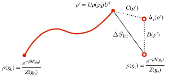
Figure 1: Irreversible work and entropy production. A system with Hamiltonian $H(g)$ is initially prepared in equilibrium at a temperature $\beta=1/T$, with $g=g_{0}$. The system is then pushed out of equilibrium by means of a work protocol $g(t)$, which lasts for a total duration $\tau$. This generates a unitary $U$ which pushes the system away from equilibrium to a state $\rho^{\prime}=U\rho(g_{0})U^{\dagger}$. The non-equilibrium nature of the process can be quantified by the irreversible work $W_{\text{irr}}$ [Eq. (2)] or, what is equivalent, the entropy production/non-equilibrium lag $\Delta S_{\text{irr}}$ in Eq. (3). This quantity, however, can be split as in Eq. (4) into a contribution $D$ [Eq. (5)] related to changes in the population and a contribution $C$ related to quantum coherence [Eq. (6)].

This typical work-protocol scenario has been the subject of countless studies, both theoretical Jarzynski (1997a, b); Derrida and Lebowitz (1998); Crooks (1998); Kurchan (1998); Lebowitz and Spohn (1999); Jarzynski (1999); Maes (1999); Jarzynski (2001); Crooks (2000); Jarzynski (2000); Mukamel (2003); Andrieux and Gaspard (2004); Monnai (2005); Teifel and Mahler (2007); Talkner et al. (2007); Kawai et al. (2007); Crooks (2008); Gelin and Kosov (2008); Jarzynski (2008); Talkner et al. (2009); Vaikuntanathan and Jarzynski (2009); Parrondo et al. (2009); Deffner and Lutz (2010); Teifel and Mahler (2011); Mazzola et al. (2013); Dorner et al. (2013); Talkner et al. (2013); Sivak and Crooks (2012); Hoppenau and Engel (2013); Watanabe et al. (2014); Roncaglia et al. (2014); Plastina et al. (2014); Skrzypczyk et al. (2014); Halpern et al. (2015); Solinas and Gasparinetti (2015); Funo et al. (2015); Alhambra et al. (2016a, b); Talkner and Hänggi (2016); Jin et al. (2016); Chenu et al. (2018); Solinas et al. (2017); Bartolotta and Deffner (2017); Park et al. (2017); Perarnau-Llobet et al. (2017); Sampaio et al. (2017); Elouard et al. (2017a); Di Stefano et al. (2017); Wei and Plenio (2017); Elouard et al. (2017b); Lostaglio (2018); Guarnieri et al. (2018); Manzano et al. (2018); Francica et al. (2019); De Chiara et al. (2019); Fusco et al. (2014a); Francica et al. (2017); Zhong and Tong (2015); Apollaro et al. (2015); Solinas and Gasparinetti (2015); del Campo et al. (2014); Brunelli et al. (2015); Allahverdyan and Nieuwenhuizen (2005); Crooks and Jarzynski (2007); Talkner et al. (2008); Deffner and Lutz (2008); Dorosz et al. (2008); Dorner et al. (2012); Ryabov et al. (2013); Carlisle et al. (2014); Roncaglia et al. (2014); Perarnau-Llobet et al. (2015); Sindona et al. (2014); Chiara et al. (2015); Arrais et al. (2018); Łobejko et al. (2017); Bayocboc and Paraan (2015) as well as experimental Liphardt et al. (2002); Douarche et al. (2005); Collin et al. (2005); Speck et al. (2007); Saira et al. (2012); Koski et al. (2013); Batalhão et al. (2014); An et al. (2014); Batalhão et al. (2015); Talarico et al. (2016); Zhang et al. (2018); Smith et al. (2018) However, although Eq. (3) is formulated for quantum systems, many aspects of it are often classical. The issue of what are the genuinely quantum features of such a process, despite still being the subject of debate, is ultimately related to the notion of quantum coherence. The thermodynamic processes involved in the map (1) highlight the energy basis as a preferred basis (in the sense of Zurek (1981)). Coherence in the energy basis therefore represents the key feature distinguishing classical and quantum processes Lostaglio et al. (2015); Santos et al. (2019). As the system is driven by the work protocol $g(t)$, the eigenbases of $H(g(t))$ at different times are not necessarily compatible, a feature which has no classical counterpart Fusco et al. (2014a).

Several results have recently appeared, which highlight the non-trivial role of coherence in irreversible thermodynamics. For instance, Ref. Miller et al. (2019); Scandi et al. (2019) considered quasi-static drives and showed how the standard fluctuation-dissipation theorem is modified to include a term related to $[H(g(t)),dH(g(t))/dt]$, thus reflecting the basis incompatibility during the drive. In Ref. Santos et al. (2019) some of us have shown that during relaxation to equilibrium, the presence of initial coherences contributes an additional term to the entropy production. A similar effect also occurs for unitary drives and the non-equilibrium lag, as shown in Francica et al. (2019). In this case, Eq. (3) may quite generally be decomposed as

$$\Delta S_{\text{irr}}=D(\rho^{\prime})+C(\rho^{\prime}).$$ (4)

The first term quantifies the contribution from changes in the population of the system and reads

$$D(\rho^{\prime})=S(\Delta_{\tau}[\rho^{\prime}]||\rho(g_{\tau})),$$ (5)

where $\Delta_{\tau}[\rho^{\prime}]$ is the completely dephased state, obtained from $\rho^{\prime}$ by eliminating its off-diagonal terms in the eigenbasis of $H(g_{\tau})$. The second term in Eq. (4), on the other hand, is the relative entropy of coherence, given by

$$C(\rho^{\prime})=S(\rho^{\prime}||\Delta_{\tau}[\rho^{\prime}])=S(\Delta_{\tau}[\rho^{\prime}])-S(\rho^{\prime}).$$ (6)

It therefore quantifies the difference between $\rho^{\prime}$ and the dephased state $\Delta_{\tau}[\rho^{\prime}]$. This term therefore measures the contribution to the non-equilibrium lag stemming solely from the quantum coherences generated by the driving protocol. Since both terms are individually non-negative by construction, this shows how coherence increases the entropy produced in the process.

In this work we will be interested in the relative contributions of the two terms in Eq. (4) in the specific case of quantum critical systems undergoing infinitesimal quenches. That is, when the control parameter changes instantaneously from $g_{0}\to g_{\tau}=g_{0}+\delta g$, where $\delta g\ll g_{0}$. As shown in Refs. Gambassi and Silva (2011); Dorner et al. (2012); Fusco et al. (2014b), the non-equilibrium lag simplifies considerably in this case, since one removes the generally complicated dependence on the exact form of the work protocol $g_{\tau}$. Notwithstanding, the problem still retains several interesting features, particularly for quantum critical systems, as beautifully shown in Refs. Dorner et al. (2012); Mascarenhas et al. (2014). This has led to a large number of studies on the critical properties of $\Delta S_{\text{irr}}$ in several models Sharma and Dutta (2015); Cosco et al. (2017); Paganelli and Apollaro (2017); Wang et al. (2018); Bayat et al. (2016); Bayocboc and Paraan (2015); Pelissetto et al. (2018); Nigro et al. (2019); Vicari (2019). A proposal to measure it experimentally in ultra-cold atoms was also given in Villa and De Chiara (2018).

None of the studies above, however, dealt with the relative contribution from populations and coherences [Eq. (4)]. How relevant is $C(\rho^{\prime})$ therefore remains unknown, even for the simplest critical models. It is the goal of this paper to fill in this gap and carry out a detailed study of the contribution from quantum coherence to the non-equilibrium lag in critical infinitesimal quenches. To accomplish this, we focus on the one-dimensional XY spin chain Lieb et al. (1961). The advantage of this model is that by tuning the anisotropy parameter one may tune the relative contribution of $C(\rho^{\prime})$ when going from the XX to the transverse field Ising model. We show that for intermediate and high temperatures, both terms in Eq. (4) contribute similarly to $\Delta S_{\text{irr}}$. At low temperatures, on the other hand, $C(\rho^{\prime})$ becomes sub-dominant. And while $D(\rho^{\prime})$ diverges logarithmically at the critical point Mascarenhas et al. (2014); Bayocboc and Paraan (2015), $C(\rho^{\prime})$ presents a cusp (i.e., its derivative is discontinuous).

II Basic setup

The Hamiltonian of the ferromagnetic $XY$ model may be written as

$$H(g,\,\gamma)=-\sum_{j=1}^{N}\bigg{(}\frac{1+\gamma}{2}\sigma_{j}^{x}\sigma_{j+1}^{x}+\frac{1-\gamma}{2}\sigma_{j}^{y}\sigma_{j+1}^{y}+g\sigma_{j}^{z}\bigg{)},$$ (7)

where $\sigma_{j}^{a}$ ($a=x,\,y,\,z$) are Pauli spin operators, $N$ is the total number of spins, $\gamma\in[0,\,1]$ is the anisotropy parameter of the spin interaction and $g$ is the applied magnetic field. We assume $N$ even, with periodic boundary conditions. This model presents a paramagnetic phase when $|g|>1$ and a ferromagnetic phase for $|g|<1$, with critical points at $g^{*}=\pm 1$. Special cases occur when one makes $\gamma=0$, to get the XX chain, and $\gamma=1$, to get the Ising model.

The Hamiltonian (7) is diagonalized by introducing the Jordan-Wigner transformation Sachdev (2011), that maps the spin chain onto an equivalent system of spinless fermions,

$$\sigma^{x}_{j}=(\hat{c}_{j}^{\dagger}+\hat{c}_{j})\prod_{i<j}(1-2\hat{c}_{i}^{\dagger}\hat{c}_{i}),$$ (8)

$$\sigma^{y}_{j}=\imath(\hat{c}_{j}^{\dagger}-\hat{c}_{j})\prod_{i<j}(1-2\hat{c}_{i}^{\dagger}\hat{c}_{i}),\quad\sigma^{z}_{j}=1-2\hat{c}_{j}^{\dagger}\hat{c}_{j},$$

where $\hat{c}_{j}^{\dagger}$ and $\hat{c}_{j}$ are canonical creation and annihilation fermionic operators. After this, one finds that the Hamiltonian (7) may be broken into two parts belonging to the orthogonal subspaces of positive and negative parity - i.e. subspaces of states with even or odd number of $c$-particles (or up spins), respectively. Each part can be independently diagonalized by a Fourier transform followed by a Bogoliubov transformation Damski and Rams (2014). However, they differ only by boundary terms which become negligible in the thermodynamic limit ($N\rightarrow\infty$). Hence, all calculations may therefore be performed considering only the positive parity subspace. We therefore consider here that, after diagonalization, we simply have

$$H(g,\,\gamma)= \sum_{k\in K^{+}}\epsilon_{k}(g,\,\gamma)\big{(}2\eta_{k}^{\dagger}\eta_{k}-1\big{)},$$ (9)

where $K^{+}=\big{\{}k=\pm(2n+1)\pi/N;\,n=0,\,1,\,2,\,...,N/2-1\big{\}}$. The dispersion relation $\epsilon_{k}(g,\,\gamma)$ is given by

$$\epsilon_{k}(g,\,\gamma)=\sqrt{[g-\cos(k)]^{2}+\gamma^{2}\sin^{2}(k)},$$ (10a)

and the canonical fermionic operators $$\{\eta_{k}\} g \gamma$$, which depend on and , are given by

$$\eta_{k}=\cos(\theta_{k}/2)\hat{c}_{k}+\sin(\theta_{k}/2)\hat{c}_{-k}^{\dagger},$$ (10b)

where

$$\Big{(}\sin\theta_{k},\,\cos\theta_{k}\Big{)}=\bigg{(}\frac{\gamma\sin(k)}{\epsilon_{k}(g,\,\gamma)},\,\frac{g-\cos(k)}{\epsilon_{k}(g,\,\gamma)}\bigg{)},$$ (10c)

and

$$\hat{c}_{j}=\frac{e^{-\imath\pi/4}}{\sqrt{N}}\sum_{k\in K^{+}}\hat{c}_{k}e^{\imath kj}.$$ (10d)

For the special case $\gamma=0$, a Bogoliubov transformation is not necessary since the Hamiltonian $H_{\gamma=0}$ becomes diagonal after the Fourier transformation (10d), and is given by

$$H_{\gamma=0}(g)=\sum_{k\in K^{+}}(g-\cos k)\big{(}2\hat{c}_{k}^{\dagger}\hat{c}_{k}-1\big{)}.$$ (11)

Our goal is to compute the entropic quantities appearing in Eqs. (5) and (6) for a quantum quench protocol. We initially consider the system to have an anisotropy parameter $\gamma_{0}$, transverse field $g_{0}$ and to be in equilibrium with a thermal reservoir at inverse temperature $\beta$. The initial state of the spin chain is therefore the thermal state $\rho(0)=e^{-\beta H(0)}/Z(0)$, with $H(0)=H(g_{0},\,\gamma_{0})$ and partition function $Z(0)=\operatorname{Tr}[e^{-\beta H(0)}]$. Thus can be further decomposed as

$$\rho(0) =\bigotimes_{\overset{k\in K^{+}}{k>0}}\rho_{\pm k}^{0},$$ (12a)

$$\rho_{\pm k}^{0} =\frac{1}{Z_{k}^{2}(0)}\sum_{n_{\pm k}=0}^{1}e^{2\beta\epsilon_{k}^{0}(1-n_{k}-n_{-k})}\arrowvert n_{-k}n_{k}\rangle\langle n_{-k}n_{k}\arrowvert,$$ (12b)

where $\arrowvert n_{-k}n_{k}\rangle$ and $\epsilon_{k}^{0}=\epsilon_{k}(g_{0},\gamma_{0})$ are the eigenstates and eigenenergies of $H(0)$ and $Z_{k}(0)=2\cosh\big{(}\beta\epsilon_{k}^{0}\big{)}$. The initial von Neumann entropy of this state is thus given by

$$S(\rho(0))=\sum_{\overset{k\in K^{+}}{k>0}}S(\rho_{\pm\,k}^{0})=2\sum_{\overset{k\in K^{+}}{k>0}}\Big{[}\ln Z_{k}(0)-\beta\epsilon_{k}^{0}\tanh\big{(}\beta\epsilon_{k}^{0}\big{)}\Big{]}.$$ (13)

At $t=0$ the system is decoupled from the thermal reservoir and undergoes a sudden quench, where the field is instantaneously changed to $g_{\tau}$ and/or the anisotropy to $\gamma_{\tau}$. The Hamiltonian therefore changes from $H(g_{0},\,\gamma_{0})$ to $H(g_{\tau},\,\gamma_{\tau})$. Moreover, since we are considering a sudden quench, the state of the system does not change, so that $\rho^{\prime}=\rho(0)$. However, since in general $[H(g_{0},\gamma_{0}),H(g_{\tau},\gamma_{\tau})]\neq 0$, the state $\rho^{\prime}$ will no longer be diagonal in the eigenbasis of $H(g_{\tau},\gamma_{\tau})$. To express $\rho^{\prime}$ in the new basis we first note that the post quench fermionic operators $\{\tilde{\eta}_{k}\}$ are related to the pre-quench operators $\{\eta_{k}\}$ according to

$$\tilde{\eta}_{k}=\eta_{k}\cos(\Delta_{k}/2)+\eta_{-k}^{\dagger}\sin(\Delta_{k}/2),$$ (14)

where $\Delta_{k}=\tilde{\theta}_{k}-\theta_{k}$ is the difference between the post- and pre-quench Bogoliubov angles (10c) and can be written as

$$\sin\Delta_{k}=\frac{\sin k}{\epsilon_{k}^{\tau}\epsilon_{k}^{0}}\big{[}\gamma_{\tau}(g_{0}-\cos k)-\gamma_{0}(g_{\tau}-\cos k)\big{]},$$ (15)

with $\epsilon_{k}^{\tau}=\epsilon_{k}(g_{\tau},\,\gamma_{\tau})$. As a consequence the pre- and post-quench eigenstates will be related by rCl |0_-k0_k⟩&=cos(Δ_k/2)|~0_-k~0_k⟩-sin(Δ_k/2)|~1_-k~1_k⟩,
|1_-k1_k⟩=sin(Δ_k/2)|~0_-k~0_k⟩+cos(Δ_k/2)|~1_-k~1_k⟩,
|0_-k1_k⟩=|~0_-k~1_k⟩,  |1_-k0_k⟩=|~1_-k~0_k⟩.

Using this in Eq. (12) we then find

$$\rho^{\prime}=\bigotimes_{\overset{k\in K^{+}}{k>0}}\tilde{\rho}_{\pm k},$$ (16)

$$\tilde{\rho}_{\pm k}=\frac{1}{Z_{k}^{2}(0)}\Bigg{\{} \arrowvert\tilde{0}_{-k}\tilde{0}_{k}\rangle\langle\tilde{0}_{-k}\tilde{0}_{k}\arrowvert\Big{[}\cosh\big{(}2\beta\epsilon_{k}^{0}\big{)}+\sinh\big{(}2\beta\epsilon_{k}^{0}\big{)}\cos\Delta_{k}\Big{]}+\arrowvert\tilde{1}_{-k}\tilde{1}_{k}\rangle\langle\tilde{1}_{-k}\tilde{1}_{k}\arrowvert\Big{[}\cosh\big{(}2\beta\epsilon_{k}^{0}\big{)}-\sinh\big{(}2\beta\epsilon_{k}^{0}\big{)}\cos\Delta_{k}\Big{]}$$

$$+ \arrowvert\tilde{0}_{-k}\tilde{1}_{k}\rangle\langle\tilde{0}_{-k}\tilde{1}_{k}\arrowvert+\arrowvert\tilde{1}_{-k}\tilde{0}_{k}\rangle\langle\tilde{1}_{-k}\tilde{0}_{k}\arrowvert-\Big{(}\arrowvert\tilde{0}_{-k}\tilde{0}_{k}\rangle\langle\tilde{1}_{-k}\tilde{1}_{k}\arrowvert+\arrowvert\tilde{1}_{-k}\tilde{1}_{k}\rangle\langle\tilde{0}_{-k}\tilde{0}_{k}\arrowvert\Big{)}\sinh(2\beta\epsilon_{k}^{0})\sin(\Delta_{k})\Bigg{\}}.$$

We now use this to compute the relative entropy of coherence in Eq. (6). The state $\Delta_{\tau}[\rho^{\prime}]$ is obtained by taking only the diagonal entries of Eq. (16). As a consequence, one readily finds that

$$S(\Delta_{\tau}[\rho^{\prime}])=\sum_{\overset{k\in K^{+}}{k>0}}\bigg{\{}2\ln Z_{k}(0)-\frac{1}{2}\tanh\big{(}\beta\epsilon_{k}^{0}\big{)}\cos(\Delta_{k})\ln\bigg{[}\frac{1+\tanh\big{(}2\beta\epsilon_{k}^{0}\big{)}\cos(\Delta_{k})}{1-\tanh\big{(}2\beta\epsilon_{k}^{0}\big{)}\cos(\Delta_{k})}\bigg{]}-\frac{\cosh\big{(}2\beta\epsilon_{k}^{0}\big{)}}{4\cosh^{2}\big{(}\beta\epsilon_{k}^{0}\big{)}}\ln\Big{[}1+\sinh^{2}\big{(}2\beta\epsilon_{k}^{0}\big{)}\sin^{2}(\Delta_{k})\Big{]}\bigg{\}},$$ (17)

Eq. (6) then follows from subtracting (13) from (17). We focus on the thermodynamic limit ($N\rightarrow\infty$), where all $k$-sums may be converted into integrals. Moreover, we study the relative entropy of coherence per particle as $\mathcal{C}(\rho^{\prime})=C(\rho^{\prime})/N$. In the limit $N\to\infty$ one then finds

$$\mathcal{C}(\rho^{\prime})=\int_{0}^{\pi}\frac{\mathrm{d}k}{2\pi}\,\Bigg{\{} \frac{1}{2}\tanh\big{(}\beta\epsilon_{k}^{0}\big{)}\Bigg{[}\ln\bigg{[}\frac{1+\tanh\big{(}2\beta\epsilon_{k}^{0}\big{)}}{1-\tanh\big{(}2\beta\epsilon_{k}^{0}\big{)}}\bigg{]}-\cos(\Delta_{k})\ln\bigg{[}\frac{1+\tanh\big{(}2\beta\epsilon_{k}^{0}\big{)}\cos(\Delta_{k})}{1-\tanh\big{(}2\beta\epsilon_{k}^{0}\big{)}\cos(\Delta_{k})}\bigg{]}\Bigg{]}-\frac{\cosh\big{(}2\beta\epsilon_{k}^{0}\big{)}}{4\cosh^{2}\big{(}\beta\epsilon_{k}^{0}\big{)}}\ln\Big{[}1+\sinh^{2}\big{(}2\beta\epsilon_{k}^{0}\big{)}\sin^{2}(\Delta_{k})\Big{]}\Bigg{\}}.$$ (18)

A similar calculation was done for the non-equilibrium lag $\Delta\mathcal{S}_{\text{irr}}=\Delta S_{\text{irr}}/N$ in Ref. Bayocboc and Paraan (2015), which found

$$\Delta\mathcal{S}_{\text{irr}}=\int_{0}^{\pi}\frac{\mathrm{d}k}{2\pi}\,2\bigg{\{}\ln\bigg{[}\frac{\cosh\big{(}\beta\epsilon_{k}^{\tau}\big{)}}{\cosh\big{(}\beta\epsilon_{k}^{0}\big{)}}\bigg{]}+\beta\big{(}\epsilon_{k}^{0}-\epsilon_{k}^{\tau}\cos(\Delta_{k})\big{)}\tanh\big{(}\beta\epsilon_{k}^{0}\big{)}\Bigg{\}}.$$ (19)

From (18) and (19), $D(\rho^{\prime})$ in Eq. (5) can be readily computed using Eq. (4). Focusing again on the contribution per particle, $\mathcal{D}(\rho^{\prime})=D(\rho^{\prime})/N$, one then finds

$$\mathcal{D}(\rho^{\prime})=\int_{0}^{\pi}\frac{\mathrm{d}k}{2\pi}\,\Bigg{\{} 2\ln\bigg{[}\frac{\cosh\big{(}\beta\epsilon_{k}^{\tau}\big{)}}{\cosh\big{(}\beta\epsilon_{k}^{0}\big{)}}\bigg{]}-\frac{1}{2}\tanh\big{(}\beta\epsilon_{k}^{0}\big{)}\cos(\Delta_{k})\Bigg{[}\ln\bigg{[}\frac{1+\tanh\big{(}2\beta\epsilon_{k}^{\tau}\big{)}}{1-\tanh\big{(}2\beta\epsilon_{k}^{\tau}\big{)}}\bigg{]}-\ln\bigg{[}\frac{1+\tanh\big{(}2\beta\epsilon_{k}^{0}\big{)}\cos(\Delta_{k})}{1-\tanh\big{(}2\beta\epsilon_{k}^{0}\big{)}\cos(\Delta_{k})}\bigg{]}\Bigg{]}$$ (20)

$$+\frac{\cosh\big{(}2\beta\epsilon_{k}^{0}\big{)}}{4\cosh^{2}\big{(}\beta\epsilon_{k}^{0}\big{)}}\ln\Big{[}1+\sinh^{2}\big{(}2\beta\epsilon_{k}^{0}\big{)}\sin^{2}(\Delta_{k})\Big{]}\Bigg{\}}.$$

As a sanity check, in the case of an XX chain ($\gamma_{0}=\gamma_{\tau}=0$) the quench does not affect the eigenbasis so $\Delta_{k}=0$. Hence, $\mathcal{C}(\rho^{\prime})=0$, and all contributions to the non-equilibrium lag stems from the changes in populations.

III High and low temperature limits

Since these results are somewhat complicated, we now proceed to separately analyze some limiting cases. As a consistency check, in all numerical analyses presented in this section, the integral expressions (18)-(20) were compared with exact numerics; i.e., obtained from discrete summations over the set $K^{+}$ [c.f. Eq. (17)] for sufficiently large $N$.

III.1 High temperature limit

For small $\beta$ (high temperatures), the expressions for $\mathcal{C}(\rho^{\prime})$, $\mathcal{D}(\rho^{\prime})$ and $\Delta\mathcal{S}_{\text{irr}}$ simplify dramatically to

$$\mathcal{C}(\rho^{\prime})=\beta^{2}\int_{0}^{\pi}\frac{\mathrm{d}k}{2\pi}\,(\epsilon_{k}^{0})^{2}\sin^{2}\Delta_{k},$$ (21a)

$$\mathcal{D}(\rho^{\prime})=\beta^{2}\int_{0}^{\pi}\frac{\mathrm{d}k}{2\pi}\,\big{(}\epsilon_{k}^{\tau}-\epsilon_{k}^{0}\cos\Delta_{k}\big{)}^{2},$$ (21b)

$$\Delta\mathcal{S}_{\text{irr}}=\beta^{2}\int_{0}^{\pi}\frac{\mathrm{d}k}{2\pi}\,\big{[}(\epsilon_{k}^{\tau})^{2}-2\epsilon_{k}^{\tau}\epsilon_{k}^{0}\cos\Delta_{k}+(\epsilon_{k}^{0})^{2}\big{]},$$ (21c)

showing that, to leading order, all quantities scale with the same order in $\beta$. Note also that these expressions do not assume the quench is infinitesimal; only that it is instantaneous. Next, let us specialize to the case of an infinitesimal quench in $g$. That is, we set $g_{\tau}=g_{0}+\delta g$, $\delta g\ll 1$ and $\gamma_{\tau}=\gamma_{0}$. In this case we get $\sin\Delta_{k}\simeq-\delta g\,\gamma_{0}\sin k/(\epsilon_{k}^{0})^{2}$ so that Eqs. (21a)-(21c) simplify to

$$\mathcal{C}(\rho^{\prime})=\beta^{2}\delta g^{2}\int_{0}^{\pi}\frac{\mathrm{d}k}{2\pi}\,\gamma_{0}^{2}\frac{\sin^{2}k}{(\epsilon_{k}^{0})^{2}},$$ (22a)

$$\mathcal{D}(\rho^{\prime})=\beta^{2}\delta g^{2}\int_{0}^{\pi}\frac{\mathrm{d}k}{2\pi}\,\frac{(g_{0}-\cos k)^{2}}{(\epsilon_{k}^{0})^{2}},$$ (22b)

$$\Delta\mathcal{S}_{\text{irr}}=\frac{1}{2}\beta^{2}\delta g^{2}.$$ (22c)

From (22a) it is clear that for this type of quench, the coherence term is maximal for the Ising model ($\gamma_{0}=1$), decreasing monotonically with $\gamma_{0}$ until it vanishes in the XX case ($\gamma_{0}=0$). In particular, for $\gamma_{0}=1$, the integral in Eq. (22a) may be evaluated analytically, to give

$$\mathcal{C}(\rho^{\prime})|_{\gamma_{0}=1}=\begin{cases}\frac{\beta^{2}\delta g^{2}}{4}&\text{for }|g_{0}|\leq 1,\\[5.69046pt] \frac{\beta^{2}\delta g^{2}}{4g_{0}^{2}}&\text{for }|g_{0}|>1.\end{cases}$$ (23)

This result is quite interesting. First, comparing with Eq. (22c), we see that when $|g_{0}|\leq 1$, half of all the non-equilibrium lag is due to quantum coherence. This is somewhat counterintuitive since this is the high-temperature limit, where one would expect quantum coherent effects to play a marginal role.

Second, and perhaps even more impressive, we see that Eq. (23) behaves differently in the two phases. And while being continuous, it presents a kink at the critical point. This behavior is plotted in Fig. 2(a). Results for $\mathcal{D}(\rho^{\prime})/\beta^{2}$ in the same range of parameters are presented in Fig. 2(b). The high-temperature behavior of the coherence term therefore reflects the nature of the quantum phase transition (which occurs at zero temperature). We are unable to provide an intuitive justification for this behavior. And to the best of our knowledge, we are unaware of any other high temperature quantities which present non-analyticities at a quantum critical point. Of course, whether this behavior is experimentally assessable is a complicated question, which has to be addressed in a case-by-case basis. In general $\mathcal{C}(\rho^{\prime})$ is not directly related to an observable, so that measuring it experimentally will in general be highly non-trivial (requiring full state tomography). However, $\mathcal{D}(\rho^{\prime})$ also presents similar signatures and, in principle, is much more easily measurable since it depends only on measurements in the energy basis.

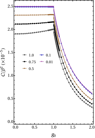
        (a)        (b)

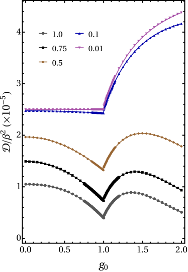
Figure 2: High temperature behavior of (a) $\mathcal{C}(\rho^{\prime})/\beta^{2}$ and (b) $\mathcal{D}(\rho^{\prime})/\beta^{2}$ as functions of $g_{0}$, computed using Eqs. (18) and (20) for quenches in $g$ with amplitude $|g_{\tau}-g_{0}|=0.01$ and fixed $\gamma_{0}=1$. Different curves correspond to different values of $\beta$. The curves in (a) approach Eq. (23) for high temperatures. Both quantities present a kink at the critical point.

We can similarly perform a quench in the anisotropy parameter, keeping $g_{\tau}=g_{0}$ and setting $\gamma_{\tau}=\gamma_{0}+\delta\gamma$. In this case we get $\sin\Delta_{k}\simeq\delta\gamma(g_{0}-\cos k)\sin k/(\epsilon_{k}^{0})^{2}$. Eqs. (21a)-(21c) then simplify to

$$\mathcal{C}(\rho^{\prime})=\beta^{2}\delta\gamma^{2}\int_{0}^{\pi}\frac{\mathrm{d}k}{2\pi}\,\frac{(g_{0}-\cos k)^{2}\sin^{2}k}{(\epsilon_{k}^{0})^{2}},$$ (24a)

$$\mathcal{D}(\rho^{\prime})=\beta^{2}\delta\gamma^{2}\int_{0}^{\pi}\frac{\mathrm{d}k}{2\pi}\,\gamma_{0}^{2}\frac{\sin^{4}k}{(\epsilon_{k}^{0})^{2}},$$ (24b)

$$\Delta\mathcal{S}_{\text{irr}}=\frac{1}{4}\beta^{2}\delta\gamma^{2}.$$ (24c)

What is interesting to note in this case is that if we initially have an XX chain, $\gamma_{0}=0$, the population mismatch due to the small quench in the anisotropy parameter vanishes, $D(\rho^{\prime})|_{\gamma_{0}=0}=0$, and all entropy production is due to coherence, independently of the value of the applied field $g_{0}$.

The above results show that there is an interplay between $\mathcal{C}$ and $\mathcal{D}$ for high temperatures, as we go from the XX to the Ising model and as we change from a quench in the field to a quench in the anisotropy. For a quench in the field, the coherence contribution to the entropy production vanishes in an XX chain and increases as we go up to the Ising model, where it reaches a maximum, contributing to half the total production of entropy. For a quench in the anisotropy, in contrast, it is $\mathcal{D}$ that vanishes in a initial XX chain, with all entropy production becoming a consequence of the generation of coherence in the quench protocol. As $\gamma_{0}$ is increased, $\mathcal{C}$ steadily decreases, reaching a minimum for the Ising model.

III.2 Low temperature limit

For large $\beta$, Eqs. (18)-(20) can be approximated by

$$\mathcal{C(\rho^{\prime})}=\int_{0}^{\pi}\frac{\mathrm{d}k}{2\pi}\,[-p_{k}\ln p_{k}-(1-p_{k})\ln(1-p_{k})],$$ (25a)

$$\mathcal{D(\rho^{\prime})}=4\beta\int_{0}^{\pi}\frac{\mathrm{d}k}{2\pi}\,\epsilon_{k}^{\tau}p_{k}-\mathcal{C}(\rho^{\prime}),$$ (25b)

$$\Delta\mathcal{S}_{\text{irr}}=4\beta\int_{0}^{\pi}\frac{\mathrm{d}k}{2\pi}\,\epsilon_{k}^{\tau}p_{k}.$$ (25c)

where $p_{k}=\sin^{2}\big{(}\Delta_{k}/2\big{)}$. Quite interestingly, the integrand in Eq. (25a) is seen to be nothing but the binary Shannon entropy associated with the two-point distribution $(p_{k},1-p_{k})$ (for each $k$). The physical interpretation of $p_{k}$ can be understood from Eq. (15), which shows that $p_{k}=\sin^{2}\big{(}\Delta_{k}/2\big{)}$ is nothing but the probability of the unoccupied (occupied) pre-quench modes $\pm k$ to become occupied (unoccupied) after the quench. With this picture in mind, the non-equilibrium lag (25c) is seen to result solely from this change in occupation, whereas the coherence reflects the entropy associated with this occupation probability.

A notable thing about Eq. (25a), is that it does not depend on $\beta$, unlike $\mathcal{D}(\rho^{\prime})$ and $\Delta\mathcal{S}_{\text{irr}}$. This means that, as the temperature is decreased, the relative contribution of $\mathcal{C}(\rho^{\prime})$ to $\Delta\mathcal{S}_{\text{irr}}$ becomes increasingly less important.

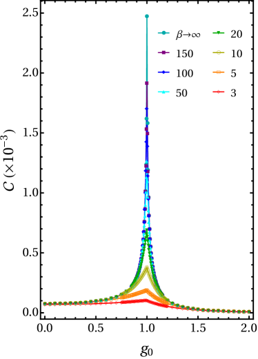
        (a)        (b)

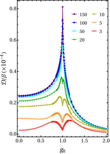
Figure 3: Low temperature behavior of (a) $\mathcal{C}(\rho^{\prime})$ and (b) $\mathcal{D}(\rho^{\prime})/\beta$ for several $\beta$ as functions of $g_{0}$, computed using Eqs. (18) and (20) for quenches in $g$ with amplitude $|g_{\tau}-g_{0}|=0.01$ and fixed $\gamma_{0}=1$. The curves in (a) approach Eq. (25a) in the limit $T=\frac{1}{\beta}\rightarrow 0$.

We start our analysis of Eqs. (25a)-(25c) by considering quenches in $g$, with $\gamma_{0}=1$ (Ising). The results are shown in Fig. 3, where we plot $\mathcal{C}(\rho^{\prime})$ and $\mathcal{D}(\rho^{\prime})/\beta$. Clearly, as $\beta\to\infty$ the latter becomes dominant. As a consequence $\Delta\mathcal{S}_{\text{irr}}\simeq\mathcal{D}(\rho^{\prime})$. This is a consequence of the fact that, in this case, changes in the Hamiltonian lead to a significant production of excitations, thus causing the contribution from populations to become dominant. Indeed, in this limit the non-equilibrium lag is known to be proportional to the magnetic susceptibility $\chi=-\partial^{2}F/\partial g_{0}^{2}$ (where $F$ is the equilibrium free energy), according to the relation Gambassi and Silva (2011); Fusco et al. (2014b)

$$\Delta\mathcal{S}_{\text{irr}}=\beta\delta g^{2}\chi.$$ (26)

As a consequence, $\Delta\mathcal{S}_{\text{irr}}/\beta\delta g^{2}$ diverges logarithmically around the critical points $|g_{0}|=1$ Paganelli and Apollaro (2017); Sharma and Dutta (2015); Mascarenhas et al. (2014). This divergence is due solely to the changes in populations.

The coherence in Fig. 3(a), on the other hand, does not diverge, which we emphasize by including a plot of $\beta\to\infty$ in Fig. 3(a). Instead, $\mathcal{C}(\rho^{\prime})$ shows a cusp at the critical point. In fact, Eq. (25a) is bounded from above by $\frac{1}{2}\ln 2$, with this maximum value occurring only for $p_{k}=1/2$ for all $k$’s. From our numerical analysis we also find that the height of the cusp at $g_{0}=1$ scales linearly with $\delta g$. The shape of the cusp in $\mathcal{C}(\rho^{\prime})$ depends on the value of $\gamma_{0}$. This is presented in Fig. 4, where we plot $\mathcal{C}(\rho^{\prime})$ for $\beta\to\infty$ for different values of $\gamma_{0}$. As can be seen, it changes from a very symmetric form for larger values of $\gamma_{0}$ to an increasingly asymmetric format as $\gamma_{0}$ decreases.

        (a)         (b)

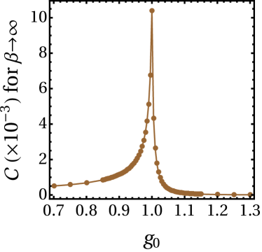
Figure 4: $\mathcal{C}(\rho^{\prime})$ vs. $g_{0}$ for $T=0$ and quenches in $g$ of magnitude $|g_{\tau}-g_{0}|=0.01$. (a) Close to the Ising case, $\gamma_{0}=0.9$ and (b) close to the XX case, $\gamma=0.2$. The curves show how the cusp of $\mathcal{C}(\rho^{\prime})$ becomes more asymmetric as $\gamma_{0}$ is reduced.

We also studied the case of quenches in the anisotropy, with fixed field. In this context, the coherence decreases with increasing $\gamma_{0}$ and has its maximal value for a vanishing field, see Fig. 5.

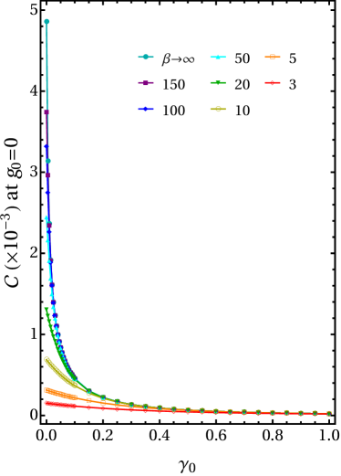
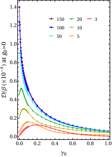
        (a)         (b)

Figure 5: Low temperature behavior of (a) $\mathcal{C}(\rho^{\prime})$ and (b) $\mathcal{D}(\rho^{\prime})/\beta$ for several $\beta$ as functions of $\gamma_{0}$, computed using Eqs. (18) and (20) for quenches in $\gamma$ with amplitude $|\gamma_{\tau}-\gamma_{0}|=0.01$ and fixed $g_{0}=0$.

III.3 Ratio $\mathcal{C}(\rho^{\prime})/\Delta\mathcal{S}_{\text{irr}}$

Next we combine the high and low temperature results and perform an analysis of the relative contribution $\mathcal{C}(\rho^{\prime})/\Delta\mathcal{S}_{\text{irr}}$. Results for quenches in $g$, with $\gamma_{0}=1$ and several values of $\beta$ are shown in Fig. 6. In the case of high temperatures, e.g. $\beta=0.1$, this fraction approaches $1/2$, which is the limit predicted by Eq. (23). Similarly, for low temperatures, the ratio tends to zero, as discussed in Sec. III.2. The notable features of Fig. 6, however, is for intermediate temperatures, where the results are not at all intuitive. First, there exists an “optimal” temperature, around $\beta\approx 2$, for which the ratio approaches unity, so that almost all entropy produced stems from coherence. This happens because as the dependence of $\mathcal{D}(\rho^{\prime})$ on $\beta$ changes from $\beta^{2}$, in the high temperature limit, to a linear dependence on $\beta$ in the low temperature limit, there is a range of temperatures in which the coherence generation for a given quench increases more rapidly than the population imbalance. Second, for large $\beta$, even though the ratio is generally small, there is nonetheless a substantial increase in the vicinity of the critical point. This is a consequence of the sharp peak in the coherence in this region, as shown in Fig. 3. However, since the coherence saturates for increasing $\beta$ while the entropy production always increases, this peak in the fraction $\mathcal{C}/\Delta\mathcal{S}_{\text{irr}}$ approaches zero as the temperature tends to zero.

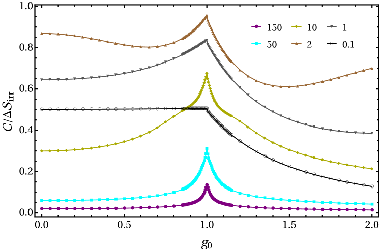
Figure 6: Ratio $\mathcal{C}/\Delta S_{\text{irr}}$ vs. $g_{0}$ for several $\beta$ and quenches in $g$ with magnitude $|g_{\tau}-g_{0}|=0.01$, with fixed $\gamma_{0}=1$. For $\beta=0.1$ the ratio approaches the limit in Eq. (23). A notable feature is the presence of an optimal temperature $\beta\approx 2$, in which almost all entropy production is due to the generation of coherence.

A similar analysis for quenches in the anisotropy parameter is shown in Fig. 7. The curve for $\beta=0.1$ show how the ratio approaches unity as $\gamma_{0}\to 0$, as previously discussed in Sec. III.1. Notably, for intermediate values of $\beta$, between $\beta=5$ to $\beta=10$, in the critical point, the coherence accounts for a large part of the production of entropy, between $25\%$ to $80\%$, for any value of the initial anisotropy. Again for large $\beta$, this ratio approaches zero.

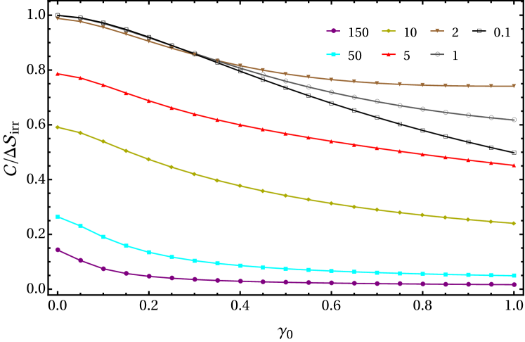
Figure 7: $\mathcal{C}(\rho^{\prime})/\Delta\mathcal{S}_{\text{irr}}$ as a function of $\gamma_{0}$ for a series of quenches in the anisotropy parameter with amplitude $|\gamma_{\tau}-\gamma_{0}|=0.01$, for several $\beta$, at $g_{0}=1$. It shows that, for small $\beta$ and $\gamma_{0}=0$, all entropy production is due to the generation of coherence for this type of quench.

IV Conclusion

We investigated the genuinely quantum-mechanical contribution of the generation of coherence to the production of entropy for quenches in the transverse field and in the anisotropy parameter of an $XY$ model. We showed that the generation of coherence is intimately related to the rotation in the basis that diagonalizes the system’s Hamiltonian when the quench protocol is performed.

For large temperatures (small $\beta=1/T$), we showed that there is an interplay between the coherent and incoherent contributions. For small quenches in the transverse field, the coherence increases steadily with the anisotropy parameter, reaching a maximum for the Ising model. For small quenches in the anisotropy, instead, we found that the coherence is the sole responsible for the entropy production if the systems starts in an XX chain. As the initial anisotropy is increased, the coherence decreases and reaches a minimum in the Ising model.

For small temperatures, we found a saturation in the contribution from coherence. This results from the fact that in such cases any change in the Hamiltonian leads to excitations on the system, which forcibly makes the production of entropy to be associated with the changes in population on the system. We also showed that the behavior of the coherence around the critical point, for quenches in the field, does not present a discontinuity, but rather a cusp. Notwithstanding, the entropy production still diverges, which is solely due to the changes in populations.

Finally, we analyzed the relative contribution of coherence to the total entropy production. For quenches in the transverse field in the Ising model, we showed that for small $\beta$ this fraction approaches $1/2$ in the ferromagnetic region. We also found that at certain temperatures the coherence can account for almost all the entropy production. For quenches in the anisotropy, the ratio of coherence to the production of entropy remains large even for intermediate $\beta$, for any initial anisotropy.

References

- Jarzynski (1997a) C. Jarzynski, Physical Review Letters 78, 2690 (1997a).
- Kurchan (1998) J. Kurchan, Journal of Physics A: Mathematical and General 31, 3719 (1998).
- Talkner et al. (2007) P. Talkner, E. Lutz, and P. Hänggi, Physical Review E 75, 050102 (2007).
- Kawai et al. (2007) R. Kawai, J. M. Parrondo, and C. Van Den Broeck, Physical Review Letters 98, 080602 (2007), arXiv:0701397 [cond-mat] .
- Vaikuntanathan and Jarzynski (2009) S. Vaikuntanathan and C. Jarzynski, EPL (Europhysics Letters) 87, 60005 (2009).
- Parrondo et al. (2009) J. M. Parrondo, C. Van Den Broeck, and R. Kawai, New Journal of Physics 11, 073008 (2009), arXiv:0904.1573 .
- Deffner and Lutz (2010) S. Deffner and E. Lutz, Physical Review Letters 105, 170402 (2010), arXiv:1005.4495 .
- Batalhão et al. (2015) T. B. Batalhão, A. M. Souza, R. S. Sarthour, I. S. Oliveira, M. Paternostro, E. Lutz, and R. M. Serra, Physical Review Letters 115, 190601 (2015), arXiv:1502.06704v1 .
- Fermi (1956) E. Fermi, Thermodynamics (Dover Publications Inc., 1956) p. 160.
- Spohn (1978) H. Spohn, J. Math. Phys. 19, 1227 (1978).
- Breuer (2003) H. P. Breuer, Physical Review A 68, 032105 (2003), arXiv:0306047 [quant-ph] .
- Santos et al. (2019) J. P. Santos, L. C. Céleri, G. T. Landi, and M. Paternostro, Nature Quantum Information 5, 23 (2019), arXiv:1707.08946 .
- Jarzynski (1997b) C. Jarzynski, Physical Review E 56, 5018 (1997b).
- Derrida and Lebowitz (1998) B. Derrida and J. L. Lebowitz, Physical Review Letters 80, 209 (1998), arXiv:9809044 [cond-mat] .
- Crooks (1998) G. E. Crooks, Journal of Statistical Physics 90, 1481 (1998).
- Lebowitz and Spohn (1999) J. Lebowitz and H. Spohn, Journal of Statistical Physics 95, 333 (1999).
- Jarzynski (1999) C. Jarzynski, Journal of statistical physics 96, 415 (1999).
- Maes (1999) C. Maes, Journal of Statistical Physics 95, 367 (1999).
- Jarzynski (2001) C. Jarzynski, Proceedings of the National Academy of Sciences 98, 3636 (2001).
- Crooks (2000) G. E. Crooks, Physical Review E 61, 2361 (2000).
- Jarzynski (2000) C. Jarzynski, Journal of Statistical Physics 98, 77 (2000).
- Mukamel (2003) S. Mukamel, Physical Review Letters 90, 170604 (2003), arXiv:0302190 [cond-mat] .
- Andrieux and Gaspard (2004) D. Andrieux and P. Gaspard, Journal of Chemical Physics 121, 6167 (2004).
- Monnai (2005) T. Monnai, Physical Review E 72, 027102 (2005).
- Teifel and Mahler (2007) J. Teifel and G. Mahler, Physical Review E 76, 051126 (2007).
- Crooks (2008) G. E. Crooks, Journal of Statistical Mechanics: Theory and Experiment 2008, P10023 (2008).
- Gelin and Kosov (2008) M. F. Gelin and D. S. Kosov, Physical Review E 78, 011116 (2008).
- Jarzynski (2008) C. Jarzynski, The European Physical Journal B 64, 331 (2008).
- Talkner et al. (2009) P. Talkner, M. Campisi, and P. Hänggi, Journal of Statistical Mechanics: Theory and Experiment , P02025 (2009).
- Teifel and Mahler (2011) J. Teifel and G. Mahler, Physical Review E 83, 041131 (2011).
- Mazzola et al. (2013) L. Mazzola, G. De Chiara, and M. Paternostro, Physical Review Letters 110, 230602 (2013), arXiv:1301.7030 .
- Dorner et al. (2013) R. Dorner, S. R. Clark, L. Heaney, R. Fazio, J. Goold, and V. Vedral, Physical Review Letters 110, 230601 (2013).
- Talkner et al. (2013) P. Talkner, M. Morillo, J. Yi, and P. Hänggi, New Journal of Physics 15, 095001 (2013).
- Sivak and Crooks (2012) D. A. Sivak and G. E. Crooks, Physical Review Letters 108, 150601 (2012).
- Hoppenau and Engel (2013) J. Hoppenau and A. Engel, Journal of Statistical Mechanics: Theory and Experiment 2013, P06004 (2013).
- Watanabe et al. (2014) G. Watanabe, B. P. Venkatesh, P. Talkner, M. Campisi, and P. Hänggi, Physical Review E - Statistical, Nonlinear, and Soft Matter Physics 89, 032114 (2014), arXiv:1312.7104 .
- Roncaglia et al. (2014) A. J. Roncaglia, F. Cerisola, and J. P. Paz, Physical Review Letters 113, 250601 (2014).
- Plastina et al. (2014) F. Plastina, A. Alecce, T. J. G. Apollaro, G. Falcone, G. Francica, F. Galve, N. L. Gullo, and R. Zambrini, Physical Review Letters 113, 260601 (2014).
- Skrzypczyk et al. (2014) P. Skrzypczyk, A. J. Short, and S. Popescu, Nature communications 5, 4185 (2014), arXiv:1307.1558 .
- Halpern et al. (2015) N. Y. Halpern, A. J. Garner, O. C. Dahlsten, and V. Vedral, New Journal of Physics 17, 095003 (2015), arXiv:1409.3878 .
- Solinas and Gasparinetti (2015) P. Solinas and S. Gasparinetti, arXiv 92, 042150 (2015), arXiv:1504.01574v1 .
- Funo et al. (2015) K. Funo, Y. Murashita, and M. Ueda, New Journal of Physics 17, 075005 (2015), arXiv:1412.5891 .
- Alhambra et al. (2016a) Á. M. Alhambra, L. Masanes, J. Oppenheim, and C. Perry, Physical Review X 6, 041017 (2016a).
- Alhambra et al. (2016b) Á. M. Alhambra, J. Oppenheim, and C. Perry, Physical Review X 6, 041016 (2016b), arXiv:1504.00020 .
- Talkner and Hänggi (2016) P. Talkner and P. Hänggi, Physical Review E 93, 022131 (2016), arXiv:1512.02516 .
- Jin et al. (2016) F. Jin, R. Steinigeweg, H. De Raedt, K. Michielsen, M. Campisi, and J. Gemmer, Physical Review E - Statistical, Nonlinear, and Soft Matter Physics 94, 012125 (2016), arXiv:1603.02833 .
- Chenu et al. (2018) A. Chenu, I. L. Egusquiza, J. Molina-Vilaplana, and A. del Campo, Scientific Reports 8, 12634 (2018), arXiv:1711.01277 .
- Solinas et al. (2017) P. Solinas, H. J. D. Miller, and J. Anders, Physical Review A 96, 052115 (2017), arXiv:1705.10296 .
- Bartolotta and Deffner (2017) A. Bartolotta and S. Deffner, Physical Review X 8, 11033 (2017), arXiv:1710.00829 .
- Park et al. (2017) J. J. Park, S. W. Kim, and V. Vedral, (2017), arXiv:1705.01750 .
- Perarnau-Llobet et al. (2017) M. Perarnau-Llobet, E. Bäumer, K. V. Hovhannisyan, M. Huber, and A. Acin, Physical Review Letters 118, 070601 (2017), arXiv:1606.08368 .
- Sampaio et al. (2017) R. Sampaio, S. Suomela, T. Ala-Nissila, J. Anders, and T. Philbin, Physical Review A 97, 012131 (2017), arXiv:1707.06159 .
- Elouard et al. (2017a) C. Elouard, D. A. Herrera-Martí, M. Clusel, and A. Auffèves, npj Quantum Information 3, 9 (2017a), arXiv:1607.02404 .
- Di Stefano et al. (2017) P. G. Di Stefano, J. J. Alonso, E. Lutz, G. Falci, and M. Paternostro, Physical Review B 98, 144514 (2017), arXiv:1704.00574 .
- Wei and Plenio (2017) B. B. Wei and M. B. Plenio, New Journal of Physics 19, 023002 (2017), arXiv:1509.07043 .
- Elouard et al. (2017b) C. Elouard, D. Herrera-Martí, B. Huard, and A. Auffèves, Physical Review Letters 118, 260603 (2017b), arXiv:1702.01917 .
- Lostaglio (2018) M. Lostaglio, Physical Review Letters 120, 040602 (2018), arXiv:1705.05397 .
- Guarnieri et al. (2018) G. Guarnieri, N. H. Y. Ng, K. Modi, J. Eisert, M. Paternostro, and J. Goold, Physical Review E 99, 050101 (2018), arXiv:1804.09962 .
- Manzano et al. (2018) G. Manzano, J. M. Horowitz, and J. M. R. Parrondo, Physical Review X 8, 031037 (2018), arXiv:1710.00054 .
- Francica et al. (2019) G. Francica, J. Goold, and F. Plastina, Physical Review E 99, 042105 (2019), arXiv:1707.06950 .
- De Chiara et al. (2019) G. De Chiara, P. Solinas, F. Cerisola, and A. J. Roncaglia, in Thermodynamics in the quantum regime - Recent Progress and Outlook, edited by F. Binder, L. A. Correa, C. Gogolin, J. Anders, and G. Adesso (Springer International Publishing, 2019) pp. 337–362, arXiv:1805.06047 .
- Fusco et al. (2014a) L. Fusco, S. Pigeon, T. J. G. Apollaro, A. Xuereb, L. Mazzola, M. Campisi, A. Ferraro, M. Paternostro, and G. De Chiara, Physical Review X 4, 031029 (2014a).
- Francica et al. (2017) G. Francica, J. Goold, M. Paternostro, and F. Plastina, Nature Quantum Information 3, 12 (2017), arXiv:1608.00124 .
- Zhong and Tong (2015) M. Zhong and P. Tong, Physical Review E 91, 032137 (2015).
- Apollaro et al. (2015) T. J. G. Apollaro, G. Francica, M. Paternostro, and M. Campisi, Physica Scripta 2015, T165 (2015), arXiv:1406.0648 .
- del Campo et al. (2014) A. del Campo, J. Goold, and M. Paternostro, Scientific Reports 4, 6208 (2014).
- Brunelli et al. (2015) M. Brunelli, A. Xuereb, A. Ferraro, G. De Chiara, N. Kiesel, and M. Paternostro, New Journal of Physics 17, 035016 (2015), arXiv:1412.4803 .
- Allahverdyan and Nieuwenhuizen (2005) A. E. Allahverdyan and T. M. Nieuwenhuizen, Physical Review E 71, 066102 (2005), arXiv:0408697 [cond-mat] .
- Crooks and Jarzynski (2007) G. E. Crooks and C. Jarzynski, Physical Review E 75, 021116 (2007).
- Talkner et al. (2008) P. Talkner, P. S. Burada, and P. Hänggi, Physical Review E 78, 011115 (2008), arXiv:0803.2808 .
- Deffner and Lutz (2008) S. Deffner and E. Lutz, Physical Review E - Statistical, Nonlinear, and Soft Matter Physics 77, 021128 (2008), arXiv:0711.3914 .
- Dorosz et al. (2008) S. Dorosz, T. Platini, and D. Karevski, Physical Review E 77, 051120 (2008).
- Dorner et al. (2012) R. Dorner, J. Goold, C. Cormick, M. Paternostro, and V. Vedral, Physical Review Letters 109, 160601 (2012).
- Ryabov et al. (2013) A. Ryabov, M. Dierl, P. Chvosta, M. Einax, and P. Maass, Journal of Physics A: Mathematical and Theoretical 46, 075002 (2013), arXiv:1302.0976 .
- Carlisle et al. (2014) A. Carlisle, L. Mazzola, M. Campisi, J. Goold, F. L. Semião, A. Ferraro, F. Plastina, V. Vedral, G. D. Chiara, and M. Paternostro, (2014), arXiv:1403.0629v1 .
- Perarnau-Llobet et al. (2015) M. Perarnau-Llobet, K. V. Hovhannisyan, M. Huber, P. Skrzypczyk, N. Brunner, and A. Acín, Physical Review X 5, 041011 (2015), arXiv:1407.7765 .
- Sindona et al. (2014) A. Sindona, J. Goold, N. Lo Gullo, and F. Plastina, New Journal of Physics 16, 045013 (2014), arXiv:1309.2669 .
- Chiara et al. (2015) G. D. Chiara, A. J. Roncaglia, and J. P. Paz, New Journal of Physics 17, 035004 (2015), arXiv:1412.6116 .
- Arrais et al. (2018) E. G. Arrais, D. A. Wisniacki, L. C. Céleri, N. G. de Almeida, A. J. Roncaglia, and F. Toscano, Physical Review E , 012106 (2018), arXiv:1802.10559 .
- Łobejko et al. (2017) M. Łobejko, J. Łuczka, and P. Talkner, Physical Review E 95, 052137 (2017), arXiv:1702.06979 .
- Bayocboc and Paraan (2015) F. A. Bayocboc and P. N. C. Paraan, Physical Review E 92, 032142 (2015).
- Liphardt et al. (2002) J. Liphardt, S. Dumont, S. B. Smith, I. Tinoco, and C. Bustamante, Science (New York, N.Y.) 296, 1832 (2002).
- Douarche et al. (2005) F. Douarche, S. Ciliberto, a. Petrosyan, and I. Rabbiosi, Europhysics Letters (EPL) 70, 593 (2005).
- Collin et al. (2005) D. Collin, F. Ritort, C. Jarzynski, S. B. Smith, I. Tinoco, and C. Bustamante, Nature 437, 231 (2005).
- Speck et al. (2007) T. Speck, V. Blickle, C. Bechinger, and U. Seifert, Europhysics Letters (EPL) 79, 30002 (2007).
- Saira et al. (2012) O. P. Saira, Y. Yoon, T. Tanttu, M. Möttönen, D. V. Averin, and J. P. Pekola, Physical Review Letters 109, 180601 (2012), arXiv:1206.7049 .
- Koski et al. (2013) J. V. Koski, T. Sagawa, O. P. Saira, Y. Yoon, A. Kutvonen, P. Solinas, M. Möttönen, T. Ala-Nissila, and J. P. Pekola, Nature Physics 9, 644 (2013), arXiv:1303.6405 .
- Batalhão et al. (2014) T. B. Batalhão, A. M. Souza, L. Mazzola, R. Auccaise, R. S. Sarthour, I. S. Oliveira, J. Goold, G. De Chiara, M. Paternostro, and R. M. Serra, Physical Review Letters 113, 140601 (2014).
- An et al. (2014) S. An, J.-N. Zhang, M. Um, D. Lv, Y. Lu, J. Zhang, Z.-Q. Yin, H. T. Quan, and K. Kim, Nature Physics 11, 193 (2014), arXiv:1409.4485 .
- Talarico et al. (2016) M. A. Talarico, P. B. Monteiro, E. C. Mattei, E. I. Duzzioni, P. H. Souto Ribeiro, and L. C. Céleri, Physical Review A 94, 042305 (2016), arXiv:1604.07237 .
- Zhang et al. (2018) Z. Zhang, T. Wang, L. Xiang, Z. Jia, P. Duan, W. Cai, Z. Zhan, Z. Zong, J. Wu, L. Sun, Y. Yin, and G. Guo, New Journal of Physics 20, 085001 (2018), arXiv:1805.10879 .
- Smith et al. (2018) A. Smith, Y. Lu, S. An, X. Zhang, J.-N. Zhang, Z. Gong, H. T. Quan, C. Jarzynski, and K. Kim, New Journal of Physics 20, 013008 (2018), arXiv:1708.01495 .
- Zurek (1981) W. H. Zurek, Physical Review D 24, 1516 (1981).
- Lostaglio et al. (2015) M. Lostaglio, D. Jennings, and T. Rudolph, Nature communications 6, 6383 (2015), arXiv:1405.2188 .
- Miller et al. (2019) H. J. D. Miller, M. Scandi, J. Anders, and M. Perarnau-Llobet, Physical Review Letters 123, 230603 (2019), arXiv:1905.07328 .
- Scandi et al. (2019) M. Scandi, H. J. D. Miller, J. Anders, and M. Perarnau-Llobet, (2019), arXiv:1911.04306 .
- Gambassi and Silva (2011) A. Gambassi and A. Silva, “Statistics of the work in quantum quenches, universality and the critical casimir effect,” (2011), arXiv:1106.2671 [cond-mat.stat-mech] .
- Fusco et al. (2014b) L. Fusco, S. Pigeon, T. J. G. Apollaro, A. Xuereb, L. Mazzola, M. Campisi, A. Ferraro, M. Paternostro, and G. De Chiara, Phys. Rev. X 4, 031029 (2014b).
- Mascarenhas et al. (2014) E. Mascarenhas, H. Bragança, R. Dorner, M. Fran ça Santos, V. Vedral, K. Modi, and J. Goold, Phys. Rev. E 89, 062103 (2014).
- Sharma and Dutta (2015) S. Sharma and A. Dutta, Phys. Rev. E 92, 022108 (2015).
- Cosco et al. (2017) F. Cosco, M. Borrelli, P. Silvi, S. Maniscalco, and G. De Chiara, Phys. Rev. A 95, 063615 (2017).
- Paganelli and Apollaro (2017) S. Paganelli and T. J. G. Apollaro, International Journal of Modern Physics B 31, 1750065 (2017), https://doi.org/10.1142/S0217979217500655 .
- Wang et al. (2018) Q. Wang, D. Cao, and H. T. Quan, Phys. Rev. E 98, 022107 (2018).
- Bayat et al. (2016) A. Bayat, T. J. G. Apollaro, S. Paganelli, G. De Chiara, H. Johannesson, S. Bose, and P. Sodano, Phys. Rev. B 93, 201106 (2016).
- Pelissetto et al. (2018) A. Pelissetto, D. Rossini, and E. Vicari, Phys. Rev. E 97, 052148 (2018).
- Nigro et al. (2019) D. Nigro, D. Rossini, and E. Vicari, Journal of Statistical Mechanics: Theory and Experiment 2019, 023104 (2019).
- Vicari (2019) E. Vicari, Phys. Rev. A 99, 043603 (2019).
- Villa and De Chiara (2018) L. Villa and G. De Chiara, Quantum 2, 42 (2018).
- Lieb et al. (1961) E. H. Lieb, T. Schultz, and D. Mattis, Annals of Physics 16, 407 (1961).
- Sachdev (2011) S. Sachdev, Quantum Phase Transitions (Cambridge University Press, 2011).
- Damski and Rams (2014) B. Damski and M. M. Rams, Journal of Physics A: Mathematical and Theoretical 47, 025303 (2014).