A parallel-in-time approach for accelerating direct-adjoint studies

Abstract

Parallel-in-time methods are developed to accelerate the direct-adjoint looping procedure. Particularly, we utilize the Paraexp algorithm, previously developed to integrate equations forward in time, to accelerate the direct-adjoint looping that arises from gradient-based optimization. We consider both linear and non-linear governing equations and exploit the linear, time-varying nature of the adjoint equations. Gains in efficiency are seen across all cases, showing that a Paraexp based parallel-in-time approach is feasible for the acceleration of direct-adjoint studies. This signifies a possible approach to further increase the run-time performance for optimization studies that either cannot be parallelized in space or are at their limit of efficiency gains for a parallel-in-space approach.

1 Introduction

The use of direct-adjoint looping techniques to compute the extremum of an objective functional, subject to a state variable satisfying complementary governing (direct) equations, is the subject of a wide range of optimization studies. Direct-adjoint looping is a technique that originated in control theory and was pioneered in fluid dynamics by Jameson [30] to find the optimal aerofoil shape that minimizes drag. These Lagrangian optimization problems are formulated with the governing equations included as constraints. The direct (governing) equations are integrated forward in time yielding a solution for a set of control parameters. Afterwards, the adjoint equations are integrated backwards in time, providing the gradient of the objective functional with respect to the parameters. This information can then be used as part of a gradient-based optimization routine to find the extremum of the objective functional via repeated applications of this direct-adjoint loop. Recent examples include, among others, the optimization of mixing in binary fluids [13, 42, 7, 9, 8], finding the minimal seed that triggers turbulence in pipe flow [46] and determining the optimal place to ignite a diffusion flame [47].

While the inclusion of the adjoint procedure significantly speeds up the calculation of the gradient information, several complications can arise due to the use of the adjoint. Firstly, the inherently iterative nature of direct-adjoint looping can cause optimization studies performed in this manner to become prohibitively slow, despite the speedup achieved through the efficient computation of the gradient. Another complication arises when the adjoint equations depend on the direct solution. This necessarily implies that the full direct solution must be saved and injected into the adjoint equation at specific points in time to obtain accurate solutions for the adjoint variables, leading to high memory costs. To circumvent these memory costs the checkpointing library revolve [25] can be used. In this way, the direct solution is saved at various checkpoints in time, and, at the expense of recomputing the solution, the direct-adjoint loop can then be solved between checkpoints leading to a reduced memory cost. These two complications, among many others, can result in run-times that may be unfeasible for some optimization studies. Traditionally, to alleviate these problems and retain viable run-times, parallel-in-space approaches are used to speed up the calculation, examples of which include work by Pekurovsky [45], Laizet and Vassilicos [35], Kallala et al. [31]. However, when encountering problems that cannot be spatially parallelized or where the parallelization in space has reached its maximum efficiency, gains in run-time efficiency must be achieved through other means. In our study, we consider one such alternative method to accelerate scenarios where more computational power is available: parallelization in time.

A wide variety of parallel-in-time algorithms have been developed for parallelizing evolution equations, and for an in-depth review we refer the reader to the review papers of Gander [16] and Ong and Schroder [44]. These methods aim to solve an equation more efficiently in parallel through a decomposition of the time domain. As the solution of an evolution equation at a future time depends on its full previous time history, parallelizing-in-time such processes is non-trivial and several approaches have arisen to tackle this challenge. The first successful attempt to overcome this difficulty was presented in the work of Nievergelt [43] who decomposed the full time domain into subdomains and calculated the solution in parallel using a shooting method. This algorithm is direct, however, since then other shooting methods that are iterative have been developed, notably, the widely studied Parareal algorithm [37] on which several other algorithms, such as parallel-implicit-time-integrator (PITA) [12], are based. As well as shooting based methods other techniques which decompose time differently exist; decomposing space-time into subdomains in space that span the whole time domain gives rise to waveform relaxation methods [36, 15, 22, 34, 41], whereas parallelizing the solver over the whole of space-time leads to multigrid methods [29, 10, 11, 18]. Further approaches include algorithms based on diagonalizing the time-stepping matrix so that all the time-steps can be solved in parallel [38] and are known as ParaDiag algorithms (see [21] for further information).

In our study we consider the Paraexp algorithm developed by Gander and Güttel [17] which is a direct method particularly suited for hyperbolic and diffusive problems [16]. This algorithm achieves parallelization-in-time for a linear equation by isolating the homogeneous and inhomogeneous parts. The time domain is then partitioned and the inhomogeneous equations are solved on each time partition with a zero initial condition. Solving the homogeneous equations allows for propagation of the correct initial conditions throughout the domain, with the full solution obtained as a superposition of all inhomogeneous and homogeneous parts. Although the homogeneous equations can span more than one time partition, and hence more initial value problems are solved than the original problem consisted of, the fact that the homogeneous equations can often be efficiently solved via exponential time integration, examples of which can be seen in Schulze et al. [49] and Bergamaschi et al. [2], leads to an overall speedup. Furthermore, this algorithm can be extended to non-linear equations via an iterative approach [33, 19].

Parallel-in-time methods have proved to be a useful choice for parallelising direct studies, especially when spatial parallelization has saturated. For example, the work of Farhat and Chandesris [12] develops and applies PITA to fluid, structure and fluid-structure interaction problems, and the work of Bal and Maday [1] considers a non-linear extension of the Parareal algorithm and implements it on the pricing of an American put option using the Black-Scholes equation. Further to these, recently the applicability of the Parareal algorithm for accelerating the time integration of kinetic dynamos [4] and Rayleigh-Bénard convection [5] has been considered. Aside from being used to accelerate direct studies, parallel-in-time methods have also been extended to optimization studies. In the work of Günther et al. [26] and Günther et al. [27] the XBraid library, which utilizes a multigrid reduction-in-time technique [14], is extended to accelerate optimization studies. Likewise, the PFASST algorithm [10] has also been used for PDE optimization [23, 24]. In addition to these multigrid-based approaches, several optimization algorithms based on Parareal have been introduced such as in the work of Maday and Turinici [39], Maday and Turinici [40] and more recently in the algorithm ParaOpt [20].

This present work aims to accelerate direct-adjoint looping by extending the Paraexp algorithm to also include the adjoint component. We consider both linear and non-linear equations, as well as the possible inclusion of a checkpointing scheme. For the case of non-linear governing equations two algorithms are developed; one in which the direct equation is solved iteratively in parallel, and another in which the direct equation is solved in series. In both cases, the adjoint equation is solved in parallel. When the direct equation is solved in series we obtain a speedup by overlapping the direct and adjoint solutions using a particularly efficient time partition. For all algorithms we derive theoretical expressions for the speedups. Furthermore, we describe in a step-by-step fashion the developed parallel-in-time algorithms and apply them to the 2D advection-diffusion equation and viscous Burgers’ equation for the linear and nonlinear cases, respectively. In all cases we observe a marked improvement in run-time efficiency in line with the theoretical predictions.

The rest of this article is organized in the following manner; §2 gives a brief overview of adjoint-looping techniques before moving on to §3 where parallel-in-time algorithms are presented for the direct and adjoint system. Next, §4 covers the numerical implementation, and the resulting numerical experiments are compared to theoretical scalings. Finally, conclusions are offered in section §5.

2 Direct-adjoint looping

We begin by briefly outlining a general direct-adjoint problem [30]. Consider the non-linear governing (direct) equation

$$\frac{\partial{\bf q}}{\partial t}=\boldsymbol{\mathcal{N}}({\bf q},{\bf p}),\qquad{\bf q}(0)={\bf q}_{0},$$ (1)

where $\boldsymbol{\mathcal{N}}({\bf q},{\bf p})$ represents the right-hand side of an equation dependent upon the state ${\bf q}$ and parameters ${\bf p}$. We seek to minimize an objective functional $\mathcal{J}$ that also can depend on the state ${\bf q}$ and parameters ${\bf p}$. To this end, we form the Lagrangian

$$\mathcal{L}({\bf q},{\bf p})=\mathcal{J}({\bf q},{\bf p})-\left(\left\langle{\bf q}^{\dagger},\frac{\partial{\bf q}}{\partial t}-{\bf\mathcal{N}}({\bf q},{\bf p})\right\rangle+\textrm{c.c.}\right),$$ (2)

where the Lagrange multiplier ${\bf q}^{\dagger}$ is the adjoint variable. Note that we have used the abbreviation c.c. to denote the complex conjugate, which is included to ensure the Lagrangian is real valued. We take the inner products and the cost functional to be of the form

$$\left\langle{\bf a},{\bf b}\right\rangle = \int_{0}^{T}[{\bf a},{\bf b}]\;\textrm{d}t,$$ (3)

$$\left[{\bf a},{\bf b}\right] = \begin{cases}{\bf a}^{H}{\bf b},\;&\textrm{discrete case,}\\ \int_{\Omega}{\bf a}^{H}{\bf b}\;\textrm{d}V&\textrm{continuous case,}\end{cases}$$ (4)

$$\mathcal{J}(\bf{q},{\bf p},{\bf q}(T)) = \begin{cases}\int_{0}^{T}\mathcal{J}_{I}({\bf q},{\bf p})\,\textrm{d}t+\mathcal{J}_{T}({\bf p},{\bf q}(T))&\textrm{discrete case,}\\ \int_{0}^{T}\int_{\Omega}\mathcal{J}_{I}({\bf q},{\bf p})\,\textrm{d}V\textrm{d}t+\mathcal{J}_{T}({\bf p},{\bf q}(T))&\textrm{continuous case,}\end{cases}$$ (5)

where differing inner products and cost functionals are introduced for the discrete and continuous cases, respectively. In our formulation, $\Omega$ represents the spatial domain, and the cost functional is split into an integral part, $\mathcal{J}_{I}$, and a part that solely depends on the final time, $\mathcal{J}_{T}$.

To minimize our objective functional subject to the constraint that our state satisfies the governing equation (1), we must ensure that all first variations of the Lagrangian are zero. Taking the variation with respect to the conjugate adjoint variable enforces the state equation (1). Before we take the variations with respect to the adjoint variable ${\bf q}^{\dagger}$, we utilize integration by parts in time to rewrite the Lagrangian as follows

$$\mathcal{L}=\mathcal{J}+\left(-[{\bf q}^{\dagger},{\bf q}]_{0}^{T}+\left\langle\frac{\partial{\bf q}^{\dagger}}{\partial t},{\bf q}\right\rangle+\left\langle{\bf q}^{\dagger},{\bf\mathcal{N}}({\bf q},{\bf p})\right\rangle+\textrm{c.c.}\right).$$ (6)

Upon taking the variations of the Lagrangian in this form with respect to the state ${\bf q}$, we arrive at the adjoint equation

$$\frac{\partial{\bf q}^{\dagger}}{\partial t}=-\frac{\partial{\bf\mathcal{N}}({\bf q},{\bf p})}{\partial{\bf q}}^{\dagger}{\bf q}^{\dagger}-\overline{{\frac{\partial\mathcal{J}_{I}}{\partial{\bf q}}}}$$ (7)

where $\overline{(\cdot)}$ denotes the complex conjugate. The adjoint operator must be found such that the adjoint relation

$$\left[{\bf a},\frac{\partial{\bf\mathcal{N}}({\bf q},{\bf p})}{\partial{\bf q}}{\bf b}\right]=\left[\frac{\partial{\bf\mathcal{N}}({\bf q},{\bf p})}{\partial{\bf q}}^{\dagger}{\bf a},{\bf b}\right]$$ (8)

is satisfied for all vectors $\bf{a}$ and ${\bf b}$. In the continuous case, this relation can be used to find the adjoint operator via integration by parts in space. For the discrete case, on the other hand, simple linear algebra manipulations can be used to find the adjoint operator

$$\frac{\partial{\bf\mathcal{N}}({\bf q},{\bf p})}{\partial{\bf q}}^{\dagger}=\frac{\partial{\bf\mathcal{N}}({\bf q},{\bf p})}{\partial{\bf q}}^{H}.$$ (9)

As the adjoint equation (7) must be integrated backwards in time from the final time $T$, we require a final time condition for the adjoint variable, ${\bf q}^{\dagger}$. This can found by ensuring the first variation with respect to ${\bf q}(T)$ is zero, i.e.,

$${\bf q}^{\dagger}(T)=\overline{\frac{\partial\mathcal{J}_{T}}{\partial{\bf q}(T)}}.$$ (10)

Finally, it remains to take the first variation with respect to ${\bf p}$. In general, unless ${\bf p}$ is a local minimum of the Lagrangian, the first variation with respect to ${\bf p}$ will be non-zero. Instead, we obtain the gradient of the Lagrangian as

$$\frac{\partial\mathcal{L}}{\partial{\bf p}}=\frac{\partial\mathcal{J}}{\partial{\bf p}}+\left\langle{\bf q}^{\dagger},\frac{\partial{\bf\mathcal{N}}({\bf q},{\bf p})}{\partial{\bf p}}\right\rangle.$$ (11)

Likewise, if the cost functional is to be optimized with respect to the initial condition, the associated gradient becomes

$$\frac{\partial\mathcal{L}}{\partial{\bf q}_{0}}=\frac{\partial\mathcal{J}}{\partial{\bf q}_{0}}+\overline{{\bf q}^{\dagger}(0)}.$$ (12)

In practice, achieving an analytic expressions for all required quantities is not feasible. Therefore, the governing equations and adjoint equations are solved explicitly, while some initial guess is employed for our control variable, ${\bf p}$ in the case of forcing or ${\bf q_{0}}$ in the case of optimal initial condition. An iterative procedure, in conjunction with either equation (11) or (12) and a gradient-descent routine, is then utilized to drive the control to a value that achieves a local minimum for the chosen cost functional.

3 Parallel-in-time algorithms

3.1 Linear governing equation

We now turn to the discussion of the parallel-in-time approach, particularly the Paraexp algorithm developed by Gander and Güttel [17]. The fundamental aspect of this approach is that a linear equation can be split into an inhomogeneous and homogeneous component. Consider the general linear equation

$$\frac{\partial{\bf q}}{\partial t}={\bf A}{\bf q}+{\bf f},\qquad{\bf q}(0)={\bf q}_{0},$$ (13)

where ${\bf q}\in\mathbb{C}^{n}$, ${\bf A}\in\mathbb{C}^{n\times n}$ and the inhomogeneity arises from the source term ${\bf f}\in\mathbb{C}^{n}$. Following Kooij et al. [33], we make the substitution $\tilde{\bf{q}}={\bf q}-{\bf q}_{0}$ to obtain the equation

$$\frac{\partial\tilde{\bf q}}{\partial t}={\bf A}\tilde{\bf q}+{\bf A}\tilde{\bf q}_{0}+{\bf f},\qquad\tilde{\bf{q}}(0)={\bf 0},$$ (14)

which absorbs the initial condition into the governing equation.

To solve this equation over the range $t\in[0,T]$ in parallel, we employ the Paraexp algorithm. For $N$ processors the time domain is decomposed into the partition $0=T_{0}<T_{1}<...<T_{N}=T$. The $p^{\textrm{th}}$ processor, where available processors are labelled $p\in\{0,1,...,N-1\}$, then solves the inhomogeneous equation

$$\frac{\partial{\bf q}_{I,p}}{\partial t}={\bf A}{\bf q}_{I,p}+{\bf A}{\bf q}_{0}+{\bf f},\qquad{\bf q}_{I,p}(T_{p})={\bf 0},$$ (15)

on $[T_{p},T_{p+1}]$. Thus the inhomogeneous part of the equation is solved on each time interval with a zero initial condition. Following this we solve the homogeneous problems

$$\frac{\partial{\bf q}_{H,j}}{\partial t}={\bf A}{\bf q}_{H,j},\qquad{\bf q}_{H,j}(T_{j})={\bf q}_{I,j-1}(T_{j}),$$ (16)

on the intervals $[T_{j},T]$ for $j\in\{1,...N-1\}$. At first it may seem that solving the equation in series would be faster than the parallel implementation, as the homogeneous components require solving over at least the interval $[T_{1},T_{N}]$, which in addition to the inhomogeneous evaluation covers the full domain. However, the speedup is achieved by recognizing that the homogeneous equations have the ability to be solved far more efficiently than the inhomogeneous equation, for example by using exponential time-stepping [48]. Hence, the slow-to-solve inhomogeneous parts are solved in parallel first and then the homogeneous parts are solved rapidly to propagate the correct initial conditions throughout the time domain. The full solution on the interval $[T_{p},T_{p+1}]$ can then be found by the sum

$${\bf q}={\bf q}_{0}+{\bf q}_{I,p}+\sum_{j=1}^{p}{\bf q}_{H,j}.$$ (17)

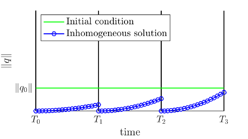
(a) First, the inhomogeneous equations are solved.

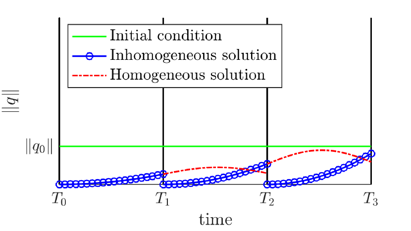
(b) Next, the homogeneous parts are solved on each processor.

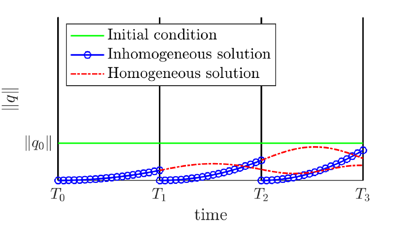
(c) The homogeneous solution on the second processor is then solved to the final time on the third processor.

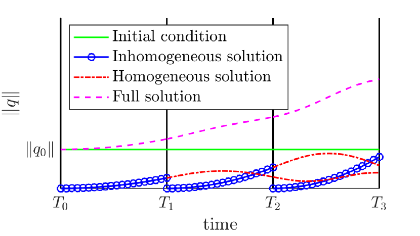
(d) Finally, we sum all parts on each processor to find the full solution.

Figure 1: An example of an equation being solved in parallel with three processors. The subfigures show the progression of the algorithm.

In their implementation of the Paraexp algorithm, Gander and Güttel [17] suggest solving problems ${\bf q}_{I,p}$ and ${\bf q}_{H,p+1}$ on the same processor so that communication between processors is only necessary when computing the sum (20) at the end. Here, however, we will consider keeping the time domain completely separate, i.e., the $p^{\textrm{th}}$ processor will always solve equations on its time partition $[T_{p},T_{p+1}]$. Therefore, whilst the inhomogeneous problems are separated by processors, an individual solution for the homogeneous part ${\bf q}_{H,j}$ will span multiple processors, resulting in necessary communications between adjacent processors. The reason for this particular arrangement is due to the inclusion of the adjoint solver. The adjoint will require full state information on each time interval and therefore it is vital for efficiency that this is available without communicating a large amount of data across processors. Hence, we rewrite the homogeneous problems (16) as

$$\frac{\partial{\bf q}_{H,p,j}}{\partial t}={\bf A}{\bf q}_{H,p,j},$$ (18)

for $p>0$ and $j\in\{0,...,p-1\}$, to be solved on $[T_{p},T_{p+1}]$ with the initial conditions

$${\bf q}_{H,p,j}(T_{p})=\begin{cases}{\bf q}_{I,p-1}(T_{p}),\;&j=0,p\neq 0,\\ {\bf q}_{H,p-1,j-1}(T_{p}),\;&1\leq j\leq p-1,p\neq 0,1.\end{cases}$$ (19)

Here the subscript $p$ completely defines the processor that the relevant equation is solved on, and the $p^{\textrm{th}}$ processor solves $p$ homogeneous problems. We note that the subscript $j$ is not the same as in equation (16) but is instead used to denote the different homogeneous problems that must be solved for each processor. Each processor (except the zero${}^{\text{th}}$) must solve the $j=0$ homogeneous problem that stems from the final time inhomogeneous state from the previous processor. Then processor $p$ must solve the additional homogeneous problems $j=1,...,(p-1)$ that arise from the homogeneous problems started on previous processors that must be integrated to the final time. By solving the equations this way the full solution on the interval $[T_{p},T_{p+1}]$ becomes

$${\bf q}={\bf q}_{0}+{\bf q}_{I,p}+\sum_{j=0,p\neq 0}^{p-1}{\bf q}_{H,p,j}.$$ (20)

It should be noted that solving the homogeneous equations in this way may introduce some lag that is not present in the Paraexp algorithm considered by Gander and Güttel [17]. This lag occurs when the homogeneous equations do not take the same time to be solved on each processor, meaning that some processors must wait to send their final states to the next processor to continue the integration. However, this introduced lag is assumed to be smaller than the cost of communicating the whole direct solution across all processors in order to solve the adjoint equations. In cases where the efficiency deterioration due to this lag becomes comparable to, or larger than, the cost of distributing the direct solution, the homogeneous solutions should be computed in the manner suggested by Gander and Güttel [17], and this is the approach considered in 3.3.

Figure 1 illustrates the progression of the algorithm for a three processor arrangement. Firstly, the inhomogeneous equations (15) are solved as displayed in figure 1(a). Figures 1(b) and 1(c) then show the homogeneous equations (18) being solved. We see the $j=0$ homogeneous states being solved on all processors in figure 1(b), with the final time solution from processor $p=1$ being passed to processor $p=2$ to solve the homogeneous state $j=1$ in figure 1(b). Finally, the sum (17) is computed on each processor to obtain the full solution.

Now that the algorithm for the direct equation has been presented we turn to the discussion on the inclusion of the adjoint solver. The adjoint equation to (13) for a given cost functional (see section 2) is

$$\frac{\partial\tilde{\bf q}^{\dagger}}{\partial t}=-{\bf A}^{H}\tilde{\bf q}^{\dagger}-{\bf A}^{H}{\bf q}^{\dagger}(T)-\overline{\frac{\partial\mathcal{J}_{I}}{\partial{\bf q}}},\qquad\;\tilde{\bf q}^{\dagger}(T)={\bf 0},$$ (21)

where we now have to integrate backwards in time, and the final time condition was absorbed into the equation using the substitution $\tilde{\bf q}^{\dagger}={\bf q}^{\dagger}-{\bf q}^{\dagger}(T)$. The linear nature of this equation means that we can use the Paraexp algorithm in exactly the same manner as previously described. The adjoint inhomogeneous problems that must be solved are

$$\frac{\partial{\bf q}^{\dagger}_{I,p}}{\partial t}=-{\bf A}^{H}{\bf q}^{\dagger}_{I,p}-{\bf A}^{H}{\bf q}^{\dagger}(T)-\overline{\frac{\partial\mathcal{J}_{I}}{\partial{\bf q}}},\qquad{\bf q}^{\dagger}_{I,p}(T_{p+1})={\bf 0},$$ (22)

on $[T_{p+1},T_{p}]$. Similarly to the direct case, the adjoint homogeneous problems are

$$\frac{\partial{\bf q}^{\dagger}_{H,j}}{\partial t}=-{\bf A}^{H}{\bf q}^{\dagger}_{H,j},\qquad{\bf q}^{\dagger}_{H,j}(T_{j+1})={\bf q}^{\dagger}_{I,j+1}(T_{j+1}),$$ (23)

on $[T_{j+1},0]$ and for $j\in\{N-2,...0\}$. Once again, we keep the adjoint homogeneous problems local to each processor’s time partition and instead solve the problems

$$\frac{\partial{\bf q}^{\dagger}_{H,p,j}}{\partial t}=-{\bf A}^{H}{\bf q}^{\dagger}_{H,p,j},$$ (24)

on $[T_{p+1},T_{p}]$ with the initial conditions

$${\bf q}^{\dagger}_{H,p,j}(T_{p+1})=\begin{cases}{\bf q}^{\dagger}_{I,p+1}(T_{p+1}),\;&j=0,p\neq N-1,\\ {\bf q}^{\dagger}_{H,p+1,j-1}(T_{p+1}),\;&1\leq j\leq(N-1)-p,\;\;p\neq N-1,N-2.\end{cases}$$ (25)

This time the $p^{\textrm{th}}$ processor solves $(N-1)-p$ homogeneous equations. Note that these equations can be solved forwards in time by making the substitution $\tau=T_{p}+T_{p+1}-t$ on each time interval. The full adjoint solution on processor $p$ is then given as the sum

$${\bf q}^{\dagger}={\bf q}^{\dagger}(T)+{\bf q}^{\dagger}_{I,p}+\sum_{j=0,p\neq N-1}^{(N-1)-p-1}{\bf q}^{\dagger}_{H,p,j},$$ (26)

on $[T_{p},T_{p+1}]$.

3.2 Non-linear governing equation solved in parallel

We now extend the parallel-in-time techniques to a direct-adjoint loop for which the governing equation is non-linear. As the adjoint equation is always a linear (and possibly linear, time-varying) equation, the Paraexp algorithm as presented in section 3.1 can always be used to solve the adjoint equation in parallel. To obtain speedup for the direct equation we present two approaches. The first uses a non-linear extension of the Paraexp algorithm, namely the method of Kooij et al. [33], to accelerate the direct equation. Note that other non-linear extensions of the Paraexp algorithm are available, see for example the proceedings of Gander et al. [19], but we do not consider them here. Specifically, the approaches of Gander et al. [19] and Kooij et al. [33] are both iterative approaches and therefore should yield fairly similar scalings.

For the non-linear governing equation we take the general equation (1) from section 2. To parallelize the time-integration of this equation we proceed using the method of Kooij et al. [33] by rewriting it in the form

$$\frac{\partial{\bf q}}{\partial t}={\bf A}{\bf q}+{\bf N}({\bf q})+{\bf f},\;{\bf q}(0)={\bf q}_{0},$$ (27)

where we have split the operator $\boldsymbol{\mathcal{N}}$ into its linear part ${\bf A}$ and genuine non-linear part ${\bf N}({\bf q})$. We then introduce the following recurrence relation

$$\frac{\partial{\bf q}_{i+1}}{\partial t}={\bf A}{\bf q}_{i+1}+{\bf N}({\bf q}_{i})+{\bf f},\qquad{\bf q}_{i+1}(0)={\bf q}_{0},$$ (28)

and note that if we achieve convergence for our series of ${\bf q}_{i}$, i.e. ${\bf q}_{i+1}\approx{\bf q}_{i}$, then (28) is equivalent to equation (27). The benefit of this altered equation is that this equation is linear in ${\bf q}_{i+1}$, as the non-linearity only acts on the previous iterate and becomes a source term only.

To achieve the convergence necessary for our recurrence relation to equate to the full equation, Kooij et al. [33] augment this equation with

$$\frac{\partial\tilde{\bf q}_{i+1}}{\partial t}=({\bf A}+{\bf J}_{i})\tilde{\bf q}_{i+1}+{\bf A}{\bf q}_{0}+{\bf N}(\tilde{\bf q}_{i})+{\bf f}-{\bf J}_{i}\tilde{\bf q}_{i},\qquad\tilde{\bf q}_{i}(0)={\bf 0},$$ (29)

where the average Jacobian

$${\bf J}_{i}=\frac{1}{T}\int_{0}^{T}\left.\frac{\partial{\bf N}({\bf q})}{\partial{\bf q}}\right|_{{\bf q}={\bf q}_{i}}\;\textrm{d}t.$$ (30)

has been added. Once again the substitution $\tilde{\bf q}={\bf q}-{\bf q}_{0}$ is used to absorb the initial condition into the equation.

The non-linear equations have now been reduced to a set of equivalent linear ones and can be solved using the Paraexp method described in the previous section, giving the inhomogeneous problems as

$$\frac{\partial{\bf q}_{I,p,i+1}}{\partial t}=({\bf A}+{\bf J}_{i,p}){\bf q}_{I,p,i+1}+{\bf A}{\bf q}_{0}+{\bf N}({\bf q}_{I,p,i})+{\bf f}-{\bf J}_{i,p}{\bf q}_{I,p,i},\;{\bf q}_{I,p,i+1}(T_{p})={\bf 0},$$ (31)

on the intervals $[T_{p},T_{p+1}]$, where the Jacobians

$${\bf J}_{i,p}=\frac{1}{T_{p+1}-T_{p}}\int_{T_{p}}^{T_{p+1}}\left.\frac{\partial{\bf N}({\bf q})}{\partial{\bf q}}\right|_{{\bf q}={\bf q}_{p,i}}\;\textrm{d}t.$$ (32)

are now averaged on each time interval. Similarly, the homogeneous equations become

$$\frac{\partial{\bf q}_{H,p,j,i+1}}{\partial t}=({\bf A}+{\bf J}_{i,p}){\bf q}_{H,p,j,i+1},$$ (33)

with the initial conditions

$${\bf q}_{H,p,j,i}(T_{p})=\begin{cases}{\bf q}_{I,p-1,i+1}(T_{p}),\;&j=0,p\neq 0,\\ {\bf q}_{H,p-1,j-1,i+1}(T_{p})\;&1\leq j\leq p-1,\;p\neq 0,1.\end{cases}$$ (34)

Once the homogeneous equations (33) are solved the next iterate of the direct solution can be found via the sum

$${\bf q}_{p,i+1}={\bf q}_{0}+{\bf q}_{I,p,i+1}+\sum_{j=1}^{p}{\bf q}_{H,p,j,+1},$$ (35)

on $[T_{p},T_{p+1}]$. One way to determine if the full non-linear solution is converged, is by iterating until $\|{\bf q}_{i+1}-{\bf q}_{i}\|<\epsilon,$ where $\epsilon$ is a user-specified tolerance. We note that caution must be used to ensure that the solution is indeed converged or whether it has merely stagnated. Possible ways to help ensure proper convergence are to require that at least a certain amount of iterations are performed, or to randomly perturb the solution after some iterations to prevent the solution from getting trapped in a ‘plateau’. However, for this study we will not consider these technicalities. Once the non-linear solution has been determined, the adjoint equation is then solved using the algorithm presented in section 3.1.

3.3 Governing equation solved in series

Whilst the previous section shows that the governing equation can be solved in parallel, problems may nevertheless arise. As there is no guarantee that the iterations will converge, it is possible that the direct solution may never be obtained. Additionally, even if the iterations do converge, the number of iterations required might outweigh the benefit obtained from solving the equation in parallel. In these cases an alternative approach is needed; we propose an algorithm in which the non-linear equation is solved in series, whilst accommodating the time-parallelization of the adjoint equation. This gives rise to the hybrid serial-direct-parallel-adjoint method presented in this section and illustrated diagrammatically in figure 2.

For the direct equation we partition the time interval so that the $p^{\textrm{th}}$ processor only solves equations on the interval $[T_{p},T_{p+1}]$. The direct equation is solved explicitly by integrating the following equations in sequence

$$\frac{\partial{\bf q}_{p}}{\partial t}=\boldsymbol{\mathcal{N}}({\bf q}_{p},{\bf f}),$$ (36)

on $[T_{p},T_{p+1}]$, with the initial conditions

$${\bf q}_{p}(T_{p})=\begin{cases}{\bf q}_{0},\;&p=0,\\ {\bf q}_{p-1}(T_{p})\;&1\leq p\leq N-1,\end{cases}$$ (37)

where the notation ${\bf q}_{p}$ is used to denote the full solution ${\bf q}$ solved on processor $p$. As the $p^{\textrm{th}}$ processor needs an initial condition from the $(p-1)^{\textrm{th}}$ processor, later processors must wait until previous processors have finished their direct solutions. However, unlike in the previous algorithms, the full direct solution is available on the interval $[T_{p},T_{p+1}]$ as each processor $p$ finishes solving equation (36). Therefore, while later processors are computing the direct solutions, earlier processors can begin solving the adjoint inhomogeneous equations. The algorithm proceeds in this manner with the direct solution being solved across all the processors, with the adjoint inhomogeneous equations beginning on each processor once the direct solution has been computed. After the adjoint inhomogeneous equations have been solved, all that remains is to compute the adjoint homogeneous equations.

In the algorithms presented previously, the initial condition for the adjoint variable was absorbed into the adjoint inhomogeneous equation. This was possible due to the adjoint solution occurring after the direct solution was calculated, and therefore the adjoint final time condition being available. However, in overlapping the direct and adjoint inhomogeneous solutions, this is not possible as the adjoint inhomogeneous solutions occur before this final time condition can be calculated. Therefore, in this case the inhomogeneous equations that must be solved are

$$\frac{\partial{\bf q}^{\dagger}_{I,p}}{\partial t}=-{\bf A}^{H}{\bf q}^{\dagger}_{I,p}-\overline{\frac{\partial\mathcal{J}_{I}}{\partial{\bf q}}},\qquad{\bf q}^{\dagger}_{I,p}(T_{p+1})={\bf 0},$$ (38)

on $[T_{p+1},T_{p}]$, i.e. the adjoint inhomogeneous equations (22) without absorbing the final time condition into them. The fact that we cannot include the effect of an adjoint final time condition directly in the equations means that we have to solve one more homogeneous problem stemming from this final time condition. Hence, in addition to solving the adjoint homogeneous problems (23), we must additionally solve

$$\frac{\partial{\bf q}^{\dagger}_{H,N-1}}{\partial t}=-{\bf A}^{H}{\bf q}^{\dagger}_{H,N-1},\qquad{\bf q}^{\dagger}_{H,N-1}(T)={\bf q}^{\dagger}(T),$$ (39)

on $[T,0]$ if there is a non-zero final time condition.

In contrast to the previous algorithms in which an equidistant time partition would be a sensible choice, the hybrid algorithm requires slightly more attention. Using the hybrid scheme means that the inhomogeneous adjoint equations start on earlier processors first. If an equidistant time partition were used, then these earlier processors would terminate first and consequently would idle for information from subsequent processors to begin solving the homogeneous adjoint equation. This time spent waiting limits the efficiency of the algorithm, as unused computing power is squandered. Therefore, it is imperative to choose the time partitioning strategically, thus avoiding the inefficiency of the equally-spaced time grid.

To prevent earlier processors waiting on later processors, all the inhomogeneous adjoint equations being solved need to terminate at the same time, i.e., the time for the full solution to be completed on one processor after having completed on the previous ones plus the subsequent adjoint inhomogeneous evaluation should remain constant on each processor. By introducing the time $\tau_{I}$ taken per time unit for the direct solve and similarly the time $\tau_{I}^{\dagger}$ taken per time unit for the adjoint inhomogeneous solve, we can write this relationship in terms of the time partition for processors $n$ and $n+1$ as

$$\underbrace{\tau_{I}\left(\sum_{i=0}^{n}(T_{i+1}-T_{i})\right)}_{\text{direct}}+\underbrace{\tau_{I}^{\dagger}(T_{n+1}-T_{n})}_{\text{adjoint}} = \underbrace{\tau_{I}\left(\sum_{i=0}^{n+1}(T_{i+1}-T_{i})\right)}_{\text{direct}}$$ (40)

$$+\underbrace{\tau_{I}^{\dagger}(T_{n+2}-T_{n+1})}_{\text{adjoint}}.$$

This relationship can be rearranged to produce

$$T_{n+2}-T_{n+1}=\frac{k}{k+1}(T_{n+1}-T_{n}).$$ (41)

with $k=\tau_{I}^{\dagger}/\tau_{I}$. This expression necessarily implies that the simultaneous termination of the inhomogeneous evaluations is achieved by making subsequent time partitions finer as we approach the final time. Equation (41) is a second-order difference equation, with boundary conditions $T_{0}=0$, and $T_{N}=T$ which can be solved to yield

$$T_{n}=T\left(\frac{1-\left(\displaystyle{\frac{k}{k+1}}\right)^{n}}{1-\left(\displaystyle{\frac{k}{k+1}}\right)^{N}}\right),$$ (42)

giving an analytic expression for the time partition in terms of the ratio $k$, which can be measured numerically.

One important difference of this hybrid serial-direct-parallel-adjoint algorithm to the previous approaches must be pointed out. In the previous cases, an equidistant time partition can be used. This means that, assuming the adjoint homogeneous equations (23) take the same amount of time to be solved on each processor, that they can be solved by instead solving the series of equations (24). This keeps the solved equations local to each processor’s time partition, meaning that the direct solution does not need to be distributed to other processors. However, in this serial-direct-parallel-adjoint approach the time partition is inherently non-equidistant. Solving the adjoint homogeneous part using the series of equations (24) will mean that later processors, which have a smaller time partition, will need to wait to pass their states to lower processors which solve equations on increasingly longer time intervals. The thus introduced lag scales with the number of processors, negating any speedup obtained from overlapping the direct and adjoint solutions. In order to circumvent this problem, the adjoint homogeneous equations must instead be solved in their original form given by equations (23) and (39). Although this means that the direct solution must be distributed to all processors, this is a one-time cost that must be paid, as it enables the algorithm to achieve an overall speedup. We choose to solve the $j^{\textrm{th}}$ adjoint homogeneous equation on processor $p$. The full adjoint solution on $[T_{p},T_{p+1}]$ can then be found by the sum

$${\bf q}^{\dagger}={\bf q}^{\dagger}(T)+{\bf q}_{I,p}^{\dagger}+\sum_{j=0}^{N-1}{\bf q}_{H,j}^{\dagger}.$$ (43)

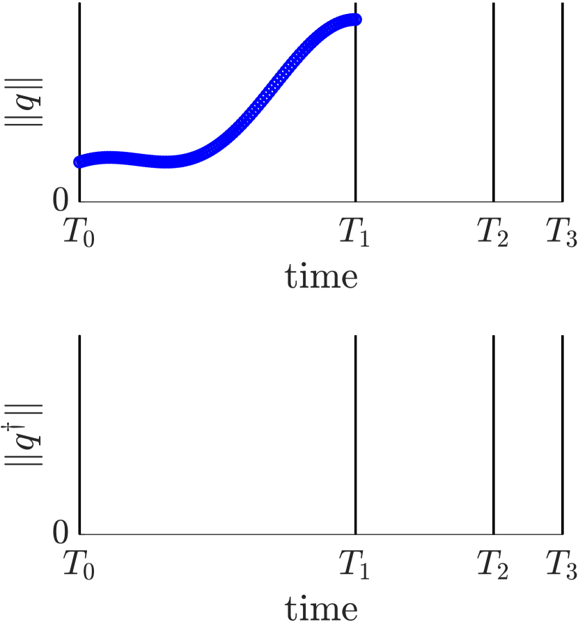
(a) First, the direct equation is solved on the zeroth processor.  

(b) Whilst the first processor takes over the direct solution, the adjoint equation begins to be solved on the zeroth processor.

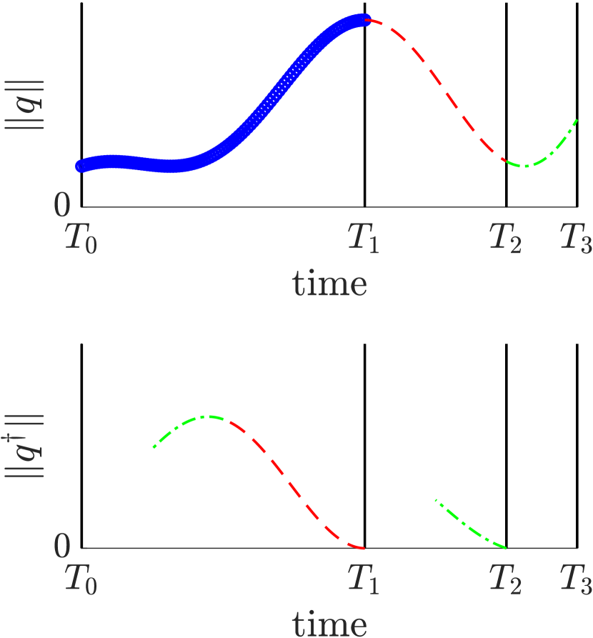
(c) The direct solution is completed on the second processor. Simultaneously, the adjoint inhomogeneous solution is continued on processor zero, and begins on processor one.

(d) Finally, all adjoint inhomogeneous solutions are completed.    

Figure 2: The overlapping of the direct solution with the adjoint inhomogeneous solutions. The colours and different line styles show which parts of the solution are completed at the same time.

Figure 2 illustrates how the hybrid algorithm plays out for a three processor arrangement. The algorithm begins by solving the direct equation for processor zero (figure 2(a)). The integration of the direct equation then continues on the next processor in figure 2(b) whilst the inhomogeneous adjoint equation begins for $p=0$. Similarly, figure 2(c) shows that, when the direct integration finishes for $p=1,$ the direct integration continues on processor two, whilst the inhomogeneous integration begins on processor one and continues on processor zero. Finally, figure 2(d) shows that after the direct integration has finished, all inhomogeneous adjoint equations terminate at the same time. The adjoint solution can then be completed by solving the homogeneous equations (23) and (39) in parallel (not shown).

3.4 Step-by-step summary of the algorithms and scaling analysis

Now that the three algorithms have been presented, we provide a step-by-step summary for ease of implementation. A scaling analysis is also conducted to assess the theoretical speedups possible.

3.4.1 Linear governing equation

Algorithm 1 Direct-adjoint loop solved in parallel for a linear governing equation

1:procedure DirectAdjointLoop(${\bf q}_{0}$,N) $\triangleright$ Perform a single direct-adjoint loop in parallel with $N$ processors

2:     Partition the time domain $[0,T]$ into $N$ equal parts $0=T_{0}<T_{1}<...<T_{N}=T$

3:     for processor $p\in\{0,...N-1\}$ do

4:         Solve equation (15) on $[T_{p},T_{p+1}]$ $\triangleright$ Direct inhomogeneous equations

5:         if $p<N-1$ then

6:              Send the state ${\bf q}_{I,p}(T_{p+1})$ to processor $p+1$$\triangleright$ communication

7:         end if

8:         if $p>0$ then

9:              Receive the state ${\bf q}_{I,p-1}(T_{p})$ from processor $p-1$$\triangleright$ communication

10:         end if

11:         for $j\in\{0,...,p-1\}$ do

12:              if $j>0$ then

13:                  Receive the state ${\bf q}_{H,p-1,j-1}(T_{p})$ from processor $p-1$

14:              end if

15:              Solve equation (24) on $[T_{p},T_{p+1}]$ $\triangleright$ Direct homogeneous equations

16:              if $j<p-1$ then

17:                  Send the direct homogeneous state ${\bf q}_{H,p,j}(T_{p+1})$ to processor $p+1$ $\triangleright$ communication

18:              end if

19:         end for

20:         Form the full direct solution on $[T_{p},T_{p+1}]$ by the sum (17)

21:         Initialize the adjoint state with the final time condition (10)

22:         Solve the adjoint inhomogeneous equation (22) on $[T_{p+1},T_{p}]$ $\triangleright$ Adjoint inhomogeneous equations

23:         if $p>0$ then

24:              Send the state ${\bf q}^{\dagger}_{I,p}(T_{p})$ to processor $p-1$ $\triangleright$ communication

25:         end if

26:         if $p<N-1$ then

27:              Receive the state ${\bf q}^{\dagger}_{I,p+1}(T_{p+1})$ from processor $p+1$ $\triangleright$ communication

28:         end if

29:         for $j\in\{0,...,N-1-p\}$ do

30:              if $j>0$ then

31:                  Receive the state ${\bf q}^{\dagger}_{H,p+1,j-1}(T_{p+1})$ from processor $p+1$

32:              end if

33:              Solve equation (24) on $[T_{p+1},T_{p}]$ $\triangleright$ Adjoint homogeneous equations

34:              if $j<N-1-p$ then

35:                  Send the state ${\bf q}^{\dagger}_{H,p,j}(T_{p})$ to processor $p-1$ $\triangleright$ communication

36:              end if

37:         end for

38:         Form the full adjoint solution on $[T_{p},T_{p+1}]$ by the sum (26)

39:     end for

40:end procedure

Algorithm 1 summarizes the linear case discussed in section 3.1. To quantify the speedup for the algorithm, we will introduce the time taken per time unit to solve the direct inhomogeneous and adjoint equations, denoted $\tau_{I}$ and $\tau_{H}$, respectively. Similarly, we introduce adjoint counterparts $\tau^{\dagger}_{I}$, $\tau^{\dagger}_{H}$. For every processor, we assume that step 4 of algorithm 1 takes the same amount of time to solve and occurs perfectly in sync. This means that the time taken to solve the inhomogeneous direct equations is $(T/N)\tau_{I}$. After the direct inhomogeneous equations are solved, the direct homogeneous equations must be solved. This is achieved by performing the for-loop beginning in step 11. Although each processor solves a different amount of direct homogeneous integrations, it is processor $N-1$ that solves the most. Therefore, the time for this loop is $(T(N-1)/N)\tau_{H}$. Hence, the total time to solve the direct equation in parallel is

$$T_{D}=\frac{T}{N}\tau_{I}+\frac{T(N-1)}{N}\tau_{H}.$$ (44)

Performing the same analysis on the adjoint part of the algorithm gives the time taken to solve the adjoint equation as

$$T_{A}=\frac{T}{N}\tau_{I}^{\dagger}+\frac{T(N-1)}{N}\tau_{H}^{\dagger}.$$ (45)

Adding the two parts together gives the total time for one direct-adjoint loop $T_{L}=T_{D}+T_{A}$ as

$$T_{L}=\frac{T}{N}(\tau_{I}+\tau_{I}^{\dagger})+\frac{T(N-1)}{N}(\tau_{H}+\tau_{H}^{\dagger}).$$ (46)

In series, the time taken for the algorithm is simply $T_{L}^{S}=T(\tau_{I}+\tau_{I}^{\dagger})$. Hence, the speedup $s=T^{S}_{L}/T_{L}$ (shown as the reciprocal speedup for convenience) is

$$s^{-1}=\frac{1}{N}+\frac{(N-1)}{N}\left(\frac{\tau_{H}+\tau_{H}^{\dagger}}{\tau_{I}+\tau_{I}^{\dagger}}\right).$$ (47)

The speedup (47) shows us that there is a theoretical maximum to the possible speedup. Indeed, as $N\rightarrow\infty$, $s\rightarrow(\tau_{I}+\tau_{I}^{\dagger})/(\tau_{H}+\tau_{H}^{\dagger})$. This highlights the importance of solving the homogeneous equation faster than the inhomogeneous equation. The faster the homogeneous integration over the inhomogeneous evaluation, the more efficient the parallel-in-time approach becomes.

3.4.2 Non-linear governing equation solved in parallel

Algorithm 2 Direct-adjoint loop solved in parallel for a non-linear governing equation

1:procedure DirectAdjointLoop(${\bf q}_{0}$,N) $\triangleright$ Perform a single direct-adjoint loop in parallel with $N$ processors

2:     Partition the time domain $[0,T]$ into $N$ equal parts $0=T_{0}<T_{1}<...<T_{N}=T$

3:     Choose a tolerance tol

4:     $\textit{err}=1e^{10}$

5:     $\textit{iter}=0$

6:     for processor $p\in\{0,...N-1\}$ do

7:         Make a guess for the direct solution ${\bf q}_{p,0}$

8:         Form the Jacobian terms by equation (32)

9:         while $\textit{err}>\textit{tol}$ do

10:              Solve equation (31) on $[T_{p},T_{p+1}]$ $\triangleright$ Direct inhomogeneous equations

11:              if $p<N-1$ then

12:                  Send the state ${\bf q}_{I,p,\textit{iter}+1}(T_{p+1})$ to processor $p+1$ $\triangleright$ communication

13:              end if

14:              if $p>0$ then

15:                  Receive the state ${\bf q}_{I,p-1,\textit{iter}+1}(T_{p})$ from processor $p-1$ $\triangleright$ communication

16:              end if

17:              for $j\in\{0,...,p-1\}$ do

18:                  if $j>0$ then

19:                       Receive the state ${\bf q}_{H,p-1,j-1,\textit{iter}+1}(T_{p})$ from processor $p-1$ $\triangleright$ communication

20:                  end if

21:                  Solve equation (33) on $[T_{p},T_{p+1}]$ $\triangleright$ Direct homogeneous equations

22:                  if $j<p-1$ then

23:                       Send the state ${\bf q}_{H,p,j,\textit{iter}+1}(T_{p+1})$ to processor $p+1$ $\triangleright$ communication

24:                  end if

25:              end for

26:              Form the current iterate of the full direct solution ${\bf q}_{p,\textit{iter}+1}$ on $[T_{p},T_{p+1}]$ by the sum (35)

27:              Form the Jacobian terms by equation (32)

28:              Calculate the error err

29:              $\textit{iter}\leftarrow\textit{iter}+1$

30:         end while

31:         Initialize the adjoint state with the final time condition (10)

32:         Solve equation (22) on $[T_{p+1},T_{p}]$ $\triangleright$ Adjoint inhomogeneous equations

33:         if $p>0$ then

34:              Send the state ${\bf q}^{\dagger}_{I,p}(T_{p})$ to processor $p-1$ $\triangleright$ communication

35:         end if

36:         if $p<N-1$ then

37:              Receive the state ${\bf q}^{\dagger}_{I,p+1}(T_{p+1})$ from processor $p+1$ $\triangleright$ communication

38:         end if

39:         for $j\in\{0,...,N-1-p\}$ do

40:              if $j>0$ then

41:                  Receive the state ${\bf q}^{\dagger}_{H,p+1,j-1}(T_{p+1})$ from processor $p+1$ $\triangleright$ communication

42:              end if

43:              Solve equation (24) on $[T_{p+1},T_{p}]$ $\triangleright$ Adjoint homogeneous equations

44:              if $j<N-1-p$ then

45:                  Send the state ${\bf q}^{\dagger}_{H,p,j}(T_{p})$ to processor $p-1$ $\triangleright$ communication

46:              end if

47:         end for

48:         Form the full adjoint solution on $[T_{p},T_{p+1}]$ by the sum (26)

49:     end for

50:end procedure

The case of a non-linear governing equation, see section 3.2, solved in parallel is summarized in algorithm 2. It has a strong resemblance to algorithm 1 except for the fact that the direct equation is now solved in an iterative fashion with the while-loop starting on line 9. For the purposes of assessing the speedup, we will include the cost of calculating the Jacobian terms on line 27 with the direct inhomogeneous equation. Furthermore, as the inhomogeneous direct equation in parallel is not the same as the direct equation in series, we introduce the time taken per time unit $\tau_{D}^{S}$ for the direct equation in series. This gives the time taken for a direct-adjoint loop in series as $T_{S}=T(\tau_{D}^{S}+\tau_{I}^{\dagger})$.

We introduce here the number of iterations $K(N)$ we require to achieve convergence for our non-linear scheme. Note the dependence of the iterations on the number of processors; the fineness of the time partition will affect the number of iterations. As each iteration involves the same steps as the linear case we obtain that the time taken for the direct equation is simply $K(N)$ times equation (44), i.e.,

$$T_{D}=K(N)\left(\frac{T}{N}\tau_{I}+\frac{T(N-1)}{N}\tau_{H}\right).$$ (48)

The time taken to solve the adjoint equation is still given by equation (45), due to the required steps being identical to algorithm 1. Hence, the time taken to perform one direct-adjoint loop in parallel is

$$T_{L}=K\left(\frac{T}{N}\tau_{I}+\frac{T(N-1)}{N}\tau_{H}\right)+\frac{T}{N}\tau_{I}^{\dagger}+\frac{T(N-1)}{N}\tau_{H}^{\dagger},$$ (49)

giving the reciprocal speedup as

$$s^{-1}=\frac{1}{N}\left(\frac{K\tau_{I}+\tau_{I}^{\dagger}}{\tau_{D}^{S}+\tau_{I}^{\dagger}}\right)+\frac{(N-1)}{N}\left(\frac{K\tau_{H}+\tau_{H}^{\dagger}}{\tau_{D}^{S}+\tau_{I}^{\dagger}}\right).$$ (50)

Equivalently to the linear case, equation (50) shows the importance of the homogeneous solvers being faster than the inhomogeneous ones. However, unlike the linear case, the factor of $K$ in the speedup equation implies that small $N$ can lead to $s<1$, signifying that no speedup is possible using a parallel approach. Requiring the speedup to be greater than one produces the condition that

$$N>\frac{K(\tau_{I}-\tau_{H})+\tau_{I}^{\dagger}-\tau_{H}^{\dagger}}{\tau_{D}^{S}+\tau_{I}^{\dagger}-\tau_{H}-K\tau_{H}^{\dagger}}.$$ (51)

Applying condition (51) to the linear case, where $K=1$ and $\tau_{D}^{S}=\tau_{I}$ simply gives the condition $N>1$, implying that a speedup is achievable for any number of processors. In the non-linear case, this no longer holds true, and $N$ must satisfy (51) in order to be faster than the serial case. Once again, the algorithm has a theoretical maximum speedup; as $N\rightarrow\infty$, $s\rightarrow(\tau_{D}^{S}+\tau_{I}^{\dagger})/(K\tau_{H}+\tau_{H}^{\dagger})$. This is similar to the linear case, except for the presence of a factor $K$ in the denominator which implies that as the number of iterations increases, the maximum speedup decreases.

3.4.3 Governing equation solved in series

Algorithm 3 Direct-adjoint loop solved in serial-direct-parallel-adjoint for a non-linear governing equation

1:procedure DirectAdjointLoop(${\bf q}_{0}$,N) $\triangleright$ Perform a single direct-adjoint loop in parallel with $N$ processors

2:     Estimate the value of $k$ in (41) by performing short direct and adjoint homogeneous calculations.

3:     Partition the time domain $[0,T]$ into $N$ parts $0=T_{0}<T_{1}<...<T_{N}=T$ using equation (42)

4:     for processor $p\in\{0,...N-1\}$ do

5:         if $p>0$ then

6:              Wait to receive the state ${\bf q}_{p-1}(T_{p})$ from processor $p-1$ $\triangleright$ communication

7:         end if

8:         Solve equation (31) on $[T_{p},T_{p+1}]$ $\triangleright$ Direct equation

9:         if $p<N-1$ then

10:              Send the direct state ${\bf q}_{p}(T_{p+1})$ to processor $p+1$ $\triangleright$ communication

11:         end if

12:         Solve the adjoint inhomogeneous equation (38) on $[T_{p+1},T_{p}]$ $\triangleright$ Adjoint inhomogeneous equations

13:     end for

14:     Scatter the direct solution to all processors $\triangleright$ communication

15:     for processor $p\in\{0,...N-1\}$ do

16:         if $p<N-1$ then

17:              Solve the $j=p^{\text{th}}$ adjoint homogeneous equation (23) on $[T_{p+1},0]$ $\triangleright$ Adjoint homogeneous equations

18:         end if

19:         if $p=N-1$ and $\mathcal{J}_{T}\neq 0$  then

20:              Solve the $j=N-1^{\text{th}}$ adjoint homogeneous equation (39) on $[T,0]$ $\triangleright$ Adjoint homogeneous equations

21:         end if

22:     end for

23:     Form the full adjoint solution with the sum (43) $\triangleright$ communication

24:end procedure

Lastly, we consider the hybrid direct-serial-parallel-adjoint case introduced in section 3.3. The procedure is summarized in algorithm 3. To obtain the speedup, we initially consider the time needed to solve the direct equation together with the adjoint inhomogeneous equations. Due to the overlapping nature of the algorithm, and the way in which we choose the non-equidistant partitioning, all inhomogeneous parts of the adjoint equation should finish at the same time. First, the direct equation is integrated in series giving a time of $\tau_{I}T$. Following this, the adjoint inhomogeneous equations must all be integrated for $(T_{N}-T_{N-1})$ time units. The time taken to finish the direct equation and the inhomogeneous adjoint equations is then $\tau_{I}T+(T_{N}-T_{N-1})\tau_{I}^{\dagger}$. Finally, the time taken to finish the direct-adjoint loop is equivalent to the time taken to solve the longest homogeneous equation, which is solved for either $T_{N-1}$ or $T$ time units depending on whether there is an adjoint final time condition. By denoting this homogeneous time as $T_{H}$ we obtain a total time for the direct-adjoint loop as

$$T_{L}=T\tau_{I}+(T_{N}-T_{N-1})\tau_{I}^{\dagger}+T_{H}\tau_{H}^{\dagger}.$$ (52)

Dividing this expression by the time it takes to solve the system in series ($T_{L}^{S}$ from the linear discussion in section (3.4.1)) gives the reciprocal speedup as

$$s^{-1}=\frac{T\tau_{I}+(T_{N}-T_{N-1})\tau_{I}^{\dagger}+T_{H}\tau_{H}^{\dagger}}{T(\tau_{I}+\tau_{I}^{\dagger})}.$$ (53)

Whilst this theoretical speedup is considerably more complicated than the other cases, we can still consider the maximum speedup achievable. We note that with the time partitioning based on equation (42), we obtain $T_{N-1}\rightarrow T$ and $(T_{N}-T_{N-1})\rightarrow 0$ as $N\rightarrow\infty$. As $T_{H}$ is either $T_{N-1}$ or $T$ we obtain $s\rightarrow(\tau_{I}+\tau_{I}^{\dagger})/(\tau_{I}+\tau_{H}^{\dagger})$, showing that effectively we achieve a speedup by replacing an inhomogeneous adjoint equation with a homogeneous one.

3.5 Checkpointing

At this point it is important to note that, owing to the addition of the forcing term in the adjoint formulation, there is an explicit dependence of the adjoint equations on the direct variables. Therefore, the direct variables need to be stored at all time steps during the forward sweep and injected, at the appropriate time, into the adjoint equations. For high-resolution cases and large time horizons, we cannot afford to store all necessary direct variables, as the memory requirements may exceed the necessary amount of RAM of our computational system. In this case a checkpointing scheme is needed.

Figure 3: Graphical representation of the checkpointing procedure.

A graphical representation of the checkpointing process, where four checkpoints $t_{1},...,t_{4}$ are used, can be seen in figure 3. Initially, the direct equation is integrated to the final checkpoint $t_{4}$ without saving any intermediate states (this run is denoted Rough in the figure). The direct equation is then integrated from the final checkpoint to the final time saving all intermediate states. As the full solution is now available between $t_{4}$ and $t_{5},$ the adjoint variable can be initialized with the relevant final time condition and integrated back to $t_{4}$. The intermediate states between $t_{4}$ and $t_{5}$ are now deleted, freeing up the RAM. This allows the direct equation to be integrated from the penultimate checkpoint $t_{3}$ to $t_{4},$ again with all intermediate states saved. The adjoint equation can then continue its backwards integration from $t_{4}$ to $t_{3}$. By continuing this checkpointing scheme backwards in this manner, the adjoint equation can be integrated back to the initial time at a fraction of the memory cost.

In view of our parallel-in-time algorithms we incorporate a checkpointing scheme as follows. We begin by defining the chosen location of our checkpoints. Then, the direct or direct-adjoint loops between each checkpoints are carried out in parallel. In this way the choice of checkpoints is independent of the choice of time-partition. For example, in the four-checkpoint example we would first carry out the direct-Rough integration by integrating in parallel (or serially in the hybrid case) the equation in the interval $[t_{0},t_{1}]$, followed by the interval $[t_{1},t_{2}]$ and so on, until the direct-Rough integration is finished. When this is accomplished, the direct-adjoint loops are performed using the parallel algorithms developed so far on the checkpointed intervals, preceding to the first time interval. Although the checkpoint times can be chosen optimally [see 25], for our numerical implementation we proceed by using equispaced checkpoints for ease of implementation.

4 Implementation details

As revealed by the scaling analysis, it is critically important that the homogeneous equations are solved faster than the inhomogeneous ones. Indeed, we can see from the theoretical scalings (47), (50) and (53) that the maximum speedup possible for each algorithm crucially depends on solving the homogeneous equation more efficiently. This implies a natural restriction on the kind of equations that we are able to parallelize in time with this approach. Utilizing the approach of Gander and Güttel [17], we identify stiff equations as good candidates for time parallelization. The homogeneous components that arise from these stiff problems can be solved efficiently and quickly with exponential time-steppers, an example of which was derived and applied to stiff equations by Cox and Matthews [6]. As exponential time-steppers are based on the exact integration of the homogeneous equation, via the matrix exponential or approximations thereof, they alleviate the stiffness of the problem and consequently are able to take larger time-steps than traditional time-stepping methods based on linear multistep or multistage formula. This section begins with a brief discussion of exponential integrators. Next, we demonstrate the application of each of the three algorithms developed to a direct-adjoint looping procedure. Special attention is given to how well the scaling of the algorithm agrees with the ones derived theoretically, and how the maximum speedup depends on the stiffness of the problem.

4.1 Exponential integrators

Exponential integration is based on the analytic solution to a linear, autonomous, homogeneous problem in terms of the matrix exponential. For the linear problem $\dot{\bf y}={\bf A}{\bf y}$ with initial condition ${\bf y}(0)={\bf y}_{0}$, the solution at time $\Delta t$ is ${\bf y}=\exp(\Delta t{\bf A}){\bf y}_{0}$. Exponential integrators rely on approximating the matrix-vector product $\exp(\Delta t{\bf A}){\bf v}$, which advances the state ${\bf v}$ by $\Delta t$ time units. Even though this approach is based on the exact integration for a linear equation, this approach can still be used for non-linear homogeneous systems, albeit with smaller time-steps. In either case, exponential time-steppers can perform better than alternative methods for stiff problems [see, e.g., 32]. A short overview of two possible exponential integrators is now given. For a more thorough review, see the recent review paper by Güttel et al. [28].

One way to approximate the matrix-vector product $\exp(\Delta t{\bf A}){\bf v}=\exp({\bf B}){\bf v}$ is via the orthogonalized, order-$m$ Krylov subspace, i.e. by forming the subspace

$$\mathcal{K}_{m}({\bf B},{\bf v})=\{{\bf v},{\bf B}{\bf v},...,{\bf B}^{m-1}{\bf v}\},$$ (54)

and orthogonalizing it [48]. By computing this subspace we can obtain a lower-dimensional representation of the matrix, namely ${\bf B}{\bf v}\approx{\bf V}_{m}{\bf H}_{m}{\bf V}_{m}^{T}{\bf v}$ where ${\bf H}_{m}$ is an $m\times m$ matrix. The product of the matrix exponential and a vector can then be approximated as $\exp({\bf B}){\bf v}\approx{\bf V}_{m}\exp({\bf H}_{m}){\bf V}_{m}^{T}{\bf v}$, which can be computed significantly more quickly and efficiently if $m$ is far smaller than the dimension of ${\bf B}$. If the Krylov representation is accurate for small $m$, then this method provides an efficient way of calculating the matrix-exponential-vector product. However, if $m$ needs to be large (e.g., if ${\bf B}$ has a large spectral radius) then this method becomes time-consuming and memory-intensive, as $m$ Krylov vectors must be calculated and stored.

An alternative to the Krylov-based method is based on Newton interpolation of the exponential function $\phi(z)=(\exp(z)-1)/z$ [3]. Once the interpolation is found, the matrix exponential $\exp({\bf B})$ can easily be retrieved from $\phi({\bf B})$. When computing the Newton interpolation the choice of interpolation points $\{\zeta_{j}\}_{j=0}^{N}$ is critically important, as a clever choice of $\zeta_{j}$ reduces the amount of points ($N+1$) needed for an accurate interpolation. One way to achieve superlinear convergence of the matrix polynomial to the matrix exponential ${\phi}({\bf Z})$ is to use Chebyshev nodes on the real focal interval $[a,b]$, computed such that ‘the “minimal” ellipse of the confocal family that contains the spectrum (or the field of values) of the matrix is not too “large” ’ [2]. However, the locations of Chebyshev nodes are dependent on the interpolation degree $N+1$. Therefore, if the interpolation degree needs to be increased in order to achieve a user-specified error, then the entire interpolation must be recomputed. This cost can be circumvented by instead using real Leja points, which still achieve a superlinear convergence. The advantage of Leja points over Chebyshev points is that they do not depend on the degree of interpolation. Hence, if a smaller error is required, the degree can be increased without recomputing the interpolation. Newton interpolation of the exponential function $\phi(z)$ is called the real Leja points method (ReLPM) and is summarized by Bergamaschi et al. [2]. In the case of large sparse matrices the ReLPM can become more advantageous over Krylov-based methods due to its lower memory cost. We choose to use the ReLPM method for our implementation so that the developed code is more easily portable to future large-scale problems. For a more detailed discussion of exponential integrators see Skene [50], which also contains a preliminary version of this work.

4.2 Linear governing equation

To test the linear algorithm 1, we consider a forced advection-diffusion equation.

$$\frac{\partial q}{\partial t}=-a\frac{\partial q}{\partial x}-a\frac{\partial q}{\partial y}+D\nabla^{2}q+f\sin(\omega t),$$ (55)

where the speed of advection is governed by $a$ and the diffusion coefficient is $D$. We take the domain to be $\Omega=[0,2\pi]\times[0,2\pi]$, and apply periodic boundary conditions in both directions. By discretizing the derivatives using second-order central differences in space we can write this equation in the discretized form

$$\frac{\text{d}{\bf q}}{\text{d}t}={\bf A}{\bf q}+{\bf f}\sin(\omega t),$$ (56)

where the vectors ${\bf q}$ and ${\bf f}$ denote the state and forcing at each grid point, respectively. The state matrix ${\bf A}$ encapsulates the homogeneous component of the original system together with the boundary conditions.

To formulate a direct-adjoint looping problem we consider choosing a force ${\bf f}={\bf f}_{\textrm{true}}$ and evolving the system over the time interval $[0,T]$ starting from a zero initial condition. This results in the solution ${\bf q}_{\textrm{true}}$. We seek to recreate the forcing ${\bf f}_{\textrm{true}}$ using only the observed solution, ${\bf q}_{\textrm{true}}$. To this end, we let the cost functional be

$$\mathcal{J}=\frac{1}{T}\int_{0}^{T}\|{\bf q}-{\bf q}_{\textrm{true}}\|^{2}\,\textrm{d}t,$$ (57)

giving the adjoint equation

$$\frac{\text{d}{\bf q}^{\dagger}(\tau)}{\text{d}\tau}={\bf A}^{T}{\bf q}^{\dagger}(\tau)+2\left({\bf q}(\tau)-{\bf q}_{\textrm{true}}(\tau)\right),$$ (58)

where we have made the substitution $\tau=T-t$ to obtain an equation we integrate forward in the time variable $\tau$. Once integrated, we can use the adjoint solution to evaluate the gradient of the cost functional with respect to the current forcing ${\bf f}$ as

$$\frac{\partial\mathcal{L}}{\partial{\bf f}}=\frac{1}{T}\int_{0}^{T}{\bf q}^{\dagger}\sin(\omega t)\,\textrm{d}t.$$ (59)

This gradient can then be used as part of a gradient-based optimization routine to minimize the cost functional and hence find ${\bf f}_{\textrm{true}}.$

As mentioned previously, the algorithms developed perform better for stiffer systems. One way of introducing stiffness into our advection-diffusion problem is through the diffusion parameter $D$. This can be observed by studying the eigenvalues of ${\bf A}$. Increasing $D$ stretches the spectrum along the negative real axis and thus makes our system progressively more stiff. For our implementation we set $a=1$, $\omega=1$, $T=10$, $f_{\textrm{true}}=\sin(x)\sin(y)$, vary $D\in\{0.01,0.1,1,10\}$ and determine the average time to perform one direct-adjoint loop over $3$ runs for a range of processor numbers. An initial guess of f=1 is used. In this manner, we can observe to what extent the theoretical scalings agree with the scalings found from the numerical experiments. We choose the final time sufficiently large so that the size of the time-steps taken by the solvers is small compared to the size of the time partitions, whilst, at the same time, small enough so that the total runtime is kept reasonable. The choice of $f_{\textrm{true}}$ and the initial guess are found to not affect the scalings obtained.

The code is written in python, and a fourth-order Runge-Kutta scheme (with adaptive time-steps based on a fifth-order Runge-Kutta error approximation) is used for the inhomogeneous integrations. This time-stepper is implemented via the inbuilt RK45 method of the solve_ivp function contained in the integrate submodule of the scipy library. For homogeneous integrations we use our implementation of the ReLPM as described by Bergamaschi et al. [2]. The relative error tolerance for each of these integrators is kept the same at $\textit{rtol}=10^{-3}.$

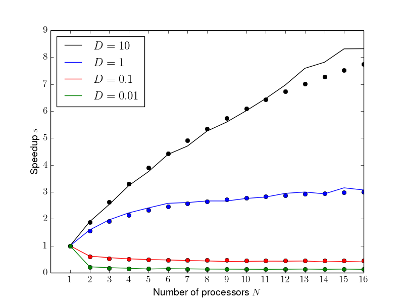
Figure 4: A figure showing the linear speedup for $D\in\{0.01,0.1,1,10\}$. The solid circles show the predicted values by the theoretical scaling formula (47).

Figure 4 shows the speedup obtained for the linear algorithm. As predicted, when $D$ increases the speedup becomes larger, highlighting the observation that the homogeneous equation needs to be solved significantly faster than the inhomogeneous one. Furthermore, due to the extra cost in forming the matrix exponential which in turn causes the homogeneous integration to be slower than the inhomogeneous one, $D=0.01$ and $D=0.1$ report a worse performance for the parallel algorithm when compared to the serial approach. For $D=1$ and $D=10$ the stiffness introduced into the system is circumvented through the exponential time-stepping and thus, for the homogeneous equation, we are able to take far larger time steps than the inhomogeneous integrator, off-setting the cost of forming the matrix exponential. This observation can be confirmed by using the values for $\tau_{H}$ and $\tau_{I}$ from the serial running. We see that for $D=0.01$ and $D=0.1$ switching to the exponential integration is around 20 and 6.67 times slower, respectively. Whereas, for $D=1$ the exponential integration is 1.5 times faster, and for $D=10$ an even larger speedup of 4.3 is found.

The figure also shows good agreement between the numerically obtained scaling and the one predicted by the theoretical value. This shows that the effectiveness of a parallel-in-time approach for a specific problem can be assessed simply by performing a short simulation to determine the parameters $\tau_{I}$, $\tau^{\dagger}_{I}$, $\tau^{\dagger}_{H}$ and , $\tau^{\dagger}_{H}$. Furthermore, by assessing the theoretical scaling the number of processors can best be chosen. In all cases, we can clearly see the scaling approaching its maximum value as the number of processors is increased. Initially, there are larger gains in speedup, followed by progressively smaller gains as more processors are included. For example, taking the $D=1$ case for instance: using six processors we can expect a speedup of roughly $2.5,$ while increasing the number of processors only provides a speed up of approximately $3$ – a relatively small speedup for more than double the number of processors. Hence, the user should initially consider the theoretical scaling and choose the number of processors that best balances speedup gains versus expended resources.

$N$		$D=0.01$		$D=0.1$		$D=1$		$D=10$
1		0.046		0.0034		0.0011		0.00061
2		0.058		0.0036		0.00087		0.0019
4		0.065		0.0088		0.0012		0.0040
8		0.074		0.020		0.0019		0.0017
16		0.089		0.0072		0.0015		0.0040

Table 1: Relative errors for the gradient obtained with a linear governing equation. The relative errors are calculated with respect to a more accurate gradient obtained in series.

To conclude our assessment of the linear algorithm we examine the error properties of performing a direct-adjoint loop in parallel. An accurate value for the gradient using equation (59) is first obtained in series using a higher error tolerance of $\textit{rtol}=10^{-8}$. Table 1 shows the relative error of the gradients computed with our lower error tolerance for different numbers of processors. We see that in general the error obtained by increasing the number of processors is not significantly different than those obtained in series. Slightly larger errors are observed when the number of processors is increased; this is in line with the original Paraexp algorithm [17]. The larger errors obtained for $D=0.01$ can be attributed to the solvers taking larger timesteps for this equation, leading to a reduced accuracy for both the interpolation of the direct equation and the computation of the gradient via numerical integration. This suggests that care must be taken to ensure that the time resolution is sufficient for computing these quantities.

4.3 Non-linear governing equation

To test the two algorithms for non-linear direct equations we consider the harmonically forced viscous Burgers’ equation

$$\frac{\partial U}{\partial t} = -U\frac{\partial U}{\partial x}-V\frac{\partial U}{\partial y}+D\nabla^{2}U+f_{U}\sin(\omega t),$$ (60)

$$\frac{\partial V}{\partial t} = -U\frac{\partial V}{\partial x}-V\frac{\partial V}{\partial y}+D\nabla^{2}V+f_{V}\sin(\omega t),$$ (61)

for the state ${\bf q}=(U,V)^{T}$ on the same domain as the advection-diffusion equation of the previous section. Once again, we discretise using second-order centered finite differences and, together with periodic boundary conditions, arrive at

$$\frac{\text{d}{\bf q}}{\text{d}t}={\mathcal{N}}({\bf q})+{\bf f}\sin(\omega t).$$ (62)

The equations linearised about the direct solution ${\bf q}=({\bf U},{\bf V})^{T}$ are

$$\frac{\partial u^{\prime}}{\partial t} = -U\frac{\partial u^{\prime}}{\partial x}-V\frac{\partial u^{\prime}}{\partial y}-u^{\prime}\frac{\partial U}{\partial x}-v^{\prime}\frac{\partial U}{\partial y}+D\nabla^{2}u^{\prime},$$ (63)

$$\frac{\partial v^{\prime}}{\partial t} = -U\frac{\partial v^{\prime}}{\partial x}-V\frac{\partial v^{\prime}}{\partial y}-u^{\prime}\frac{\partial V}{\partial x}-v^{\prime}\frac{\partial V}{\partial y}+D\nabla^{2}v^{\prime},$$ (64)

for the linearised state ${\bf q}^{\prime}=({\bf u}^{\prime},{\bf v}^{\prime})^{T}$. These equations are also discretized using second-order centered finite differences with periodic boundary conditions. This leads to the linearized equations in the form

$$\frac{\text{d}{\bf q}^{\prime}}{\text{d}t}={\bf A}(U(t),V(t)){\bf q}^{\prime},$$ (65)

with the corresponding adjoint equation

$$\frac{\text{d}{\bf q}^{\dagger}}{\text{d}\tau}={\bf A}^{T}(U(\tau),V(\tau)){\bf q}^{\dagger}+2({\bf q}(\tau)-{\bf q}_{\textrm{true}}(\tau)).$$ (66)

We have made explicit the dependence of the state matrix ${\bf A}$ on the direct solution and have, as before, introduced the time variable $\tau=T-t$ to integrate the adjoint equations forwards in the time variable $\tau$. The parameters chosen are $T=1$, $\omega=1$ and $f_{U,\textrm{true}}=f_{V,\textrm{true}}=\sin(x)\sin(y)$ with an initial guess of $f_{U}=f_{V}=1$. Again, the choice of ${\bf f}_{\textrm{true}}$ and the initial guess are found to not affect the results.

4.3.1 Non-linear governing equation solved in parallel

Now we turn to timing the direct-adjoint loop, i.e., we solve both the non-linear governing equation and the adjoint in parallel as described by algorithm 2. Figure 5 shows the comparison between the numerically obtained speedup and the speedup predicted by our theoretical scaling (50). As four iterations are used to converge the direct solution, we set $K=4$ when computing the theoretical scaling.

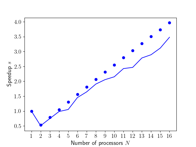
Figure 5: Non-linear speedup with the iterative procedure for $D=1$. The solid circles show the predicted values by the theoretical scaling formula (50).

We note again that there is good agreement between the numerically obtained speedup and that predicted by our theoretical arguments. Initially the speedup is less than one due to the cost of performing four iterations negating any possible speedup. However, for $N>4$ this cost is overcome, and we obtain a marked speedup.

4.3.2 Non-linear governing equation solved in series

Next, we time the same direct-adjoint loop, but using algorithm 3 in which the direct equation is solved in series. By performing short direct and adjoint simulations we obtain the value $k=2.11$ for calculating the size of the time partitions using equation (42). The speedup obtained, compared to the theoretical value, is shown in figure 6.

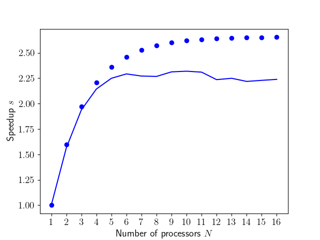
Figure 6: Non-linear speedup with the hybrid procedure for $D=1$. The solid circles show the predicted values by the theoretical scaling formula (53).

The figure shows that the speedup converges to its theoretical maximum much faster than in the previous two algorithms. Indeed, about four processors are needed for the speedup to obtain its theoretical maximum. We also see a larger discrepancy in the obtained maximum efficiency gain and the one predicted by our scaling equation. This can mainly be attributed to the fact that the scaling argument assumes that, as the width of the time partition gets smaller, the inhomogeneous and homogeneous equations can be solved increasingly faster. However, for our non-equispaced time partitioning, there comes a point in which the time partition becomes smaller than the minimum time-step needed to solve the equation. Hence, decreasing the width of the time partition beyond this point does not yield any speedup in solving the equation.

$N$		iterative		hybrid
1		0.0030		0.0030
2		0.0044		0.0027
4		0.0030		0.0033
8		0.0057		0.0028
16		0.0097		0.0029

Table 2: Relative errors for the gradient obtained with a non-linear governing equation. The relative errors are calculated with respect to a more accurate gradient obtained in series with a relative tolerance of $\textit{rtol}=10^{-8}$.

Similarly to the linear case, table 2 shows the errors for the gradients obtained for the non-linear equation. Again, we see that increasing the number of processors does not change the error appreciably compared to the serial case. Interestingly, the error obtained with the hybrid algorithm stays more constant than for the case of solving the non-linear equation in parallel. This is to be expected as there is an increased source of error for non-linear equations stemming from solving the equation iteratively which is off-set by using the hybrid algorithm.

4.4 Checkpointing

Lastly, we turn our attention to the inclusion of a checkpointing scheme in performing a direct-adjoint loop. We consider the same problem as in section 4.3.2, but we include five checkpoints using the method outlined in section 3.5. The speedup obtained is shown in figure 7.

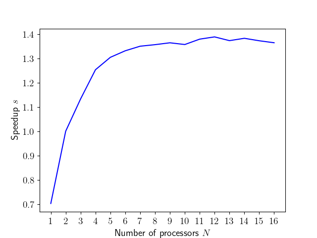
Figure 7: Non-linear speedup with the hybrid procedure for $D=1$ when five checkpoints are used.

Similarly to the hybrid example with no checkpoints, we obtain the maximum speedup at about four processors. The maximum speedup has decreased, but this is to be expected for the hybrid algorithm as no speedup is gained in solving the forward equation by itself. Only direct-adjoint loops are accelerated. The fact that a speedup is still obtained with the inclusion of checkpoints demonstrates the compatibility of our developed algorithms with checkpointing schemes. For the cases of a linear governing equation, and a non-linear direct equation solved in parallel, we can expect less of a penalty for using a checkpointing scheme as, in this case, the forward equations are also accelerated.

5 Conclusions

In this article we have presented three separate algorithms that aim to extend the Paraexp algorithm of Gander and Güttel [17] to adjoint-looping studies. Theoretical speed-ups have been derived for all cases and verified through a set of numerical experiments. The verifications of the theoretical predictions indicate that studies utilizing these approaches can a-priori assess the achievable speedups as well as the necessary processors required. All algorithms sped up the calculation of the relevant system in line with the predictions we presented, signifying that the adjoint Paraexp algorithm, and its non-linear extension, can be used to accelerate direct-adjoint optimization studies. This is particularly pertinent due to the linear, time-varying nature of the adjoint which lends itself naturally to this parallelization approach, and thus can always be parallelized in time.

We first considered the extension of the Paraexp algorithm to direct-adjoint loops that stem from a linear governing equation. As the adjoint equation is also a linear equation this can be achieved simply by integrating the adjoint equation using the Paraexp algorithm. By keeping solutions on each time partition local to each processor we were able to minimize the processor communications required for direct-adjoint looping. The theoretical scaling of the algorithm was derived, showing that this algorithm has a theoretical maximum that can be obtained as the number of processors is increased. The linear algorithm was demonstrated on a two-dimensional advection-diffusion equation, where good agreement with theoretical scalings was obtained. These numerical experiments, as well as the theoretical scalings, highlight an important consideration that must be made when using the Paraexp algorithm, namely that the stiffness of the governing equations should be taken into account. Only when the homogeneous component can be solved significantly faster than the inhomogeneous one, can speedups be obtained. Keeping this caveat in mind, we expect this approach to be particularly applicable to systems governing by a stiff (multi-scale) dynamics.

Further to the linear case, we also considered how a parallel-in-time approach can be used for non-linear direct equations. This led to the development of two algorithms; an iterative algorithm in which the direct equation is solved in parallel, and a hybrid algorithm in which the direct equation is solved in series. In both cases the adjoint equation is integrated in parallel using the Paraexp algorithm. The scalings for the iterative approach showed that due to iterations being carried out, care must be taken to ascertain whether a speedup is possible for a given number of processors as the cost of iterations can readily outweigh the cost of solving the equations in parallel. Also, similarly to the linear case, there is a maximum speedup possible. Therefore, an initial analysis of the governing equations may be necessary to ascertain if this approach is applicable and viable.

As in the iterative non-linear algorithm the iterations may not converge, or too many processors may be needed in order to obtain a speedup, we also proposed a hybrid approach in which the direct equation is solved in series whilst the adjoint is solved in parallel. By using a non-equidistant time-partitioning and overlapping the direct and adjoint solves, a speedup can be obtained. The time-partitioning is chosen so that all the homogeneous adjoint solves begin at the same time. In this way, the theoretical scaling shows that, as the number of processors increases, we obtain a maximum speedup where the inhomogeneous adjoint integration is effectively replaced by a homogeneous one. The scaling and subsequent numerical verification demonstrated that in this approach the maximum speedup, although lower than the other algorithms, is obtained with a smaller number of processors. Again, we note that for the non-linear algorithms the speedups rely on the homogeneous equations being able to be solved more efficiently than their inhomogeneous counterparts, for example as in the case of a stiff system.

Lastly, we demonstrated that all developed algorithms are easily implementable with checkpointing regimes. Hence, we believe that a Paraexp based parallel-in-time approach can provide a viable option for accelerating direct-adjoint loops stemming from both linear and non-linear governing equations, with the theoretical scalings providing an easy ‘a-priori check’ of the speedups available. We emphasise that this approach is particularly aimed at studies that have exhausted spatial parallelization but still have additional computational power available. In this case, a significant impact can be made by parallelizing in time, adding valuable efficiency to these optimization studies. The optimal overall balance of spatial versus temporal parallelism for a given number of processors and a given computer architecture is an interesting extension of our study and will be addressed in a future effort.

References

- Bal and Maday [2002] G. Bal and Y. Maday. A “parareal” time discretization for non-linear pde’s with application to the pricing of an American put. In Recent Developments in Domain Decomposition Methods, pages 189–202, Berlin, Heidelberg, 2002. Springer Berlin Heidelberg.
- Bergamaschi et al. [2006] L. Bergamaschi, M. Caliari, A. Martínez, and M. Vianello. Comparing Leja and Krylov approximations of large scale matrix exponentials. In Computational Science – ICCS 2006, volume 3994 of Lect. Notes in Comp. Sci., pages 685–692, Berlin, Heidelberg, 2006. Springer-Verlag.
- Caliari [2007] M. Caliari. Accurate evaluation of divided differences for polynomial interpolation of exponential propagators. Computing, 80(2):189–201, 2007.
- Clarke et al. [2020a] A. T. Clarke, C. J. Davies, D. Ruprecht, and S. M. Tobias. Parallel-in-time integration of kinematic dynamos. Journal of Computational Physics: X, 7:100057, 2020a.
- Clarke et al. [2020b] A. T. Clarke, C. J. Davies, D. Ruprecht, S. M. Tobias, and J. S. Oishi. Performance of parallel-in-time integration for Rayleigh Bénard convection. Computing and Visualization in Science, 23(1):10, 2020b.
- Cox and Matthews [2002] S. M. Cox and P. C. Matthews. Exponential time differencing for stiff systems. J. Comp. Phys., 176(2):430–455, 2002.
- Eggl and Schmid [2018] M. F. Eggl and P. J. Schmid. A gradient-based framework for maximizing mixing in binary fluids. J. Comp. Phys., 368:131–153, 2018.
- Eggl and Schmid [2020a] M. F. Eggl and P. J. Schmid. Mixing enhancement in binary fluids using optimised stirring strategies. Journal of Fluid Mechanics, 899:A24, 2020a.
- Eggl and Schmid [2020b] M. F. Eggl and P. J Schmid. Shape optimization of stirring rods for mixing binary fluids. IMA Journal of Applied Mathematics, pages 762–789, 2020b.
- Emmett and Minion [2012] M. Emmett and M. L. Minion. Toward an Efficient Parallel in Time Method for Partial Differential Equations. Communications in Applied Mathematics and Computational Science, 7:105–132, 2012.
- Falgout et al. [2014] R. D. Falgout, S. Friedhoff, Tz. V. Kolev, S. P. MacLachlan, and J. B. Schroder. Parallel time integration with multigrid. SIAM Journal on Scientific Computing, 36(6):C635–C661, 2014.
- Farhat and Chandesris [2003] C. Farhat and M. Chandesris. Time-decomposed parallel time-integrators: theory and feasibility studies for fluid, structure, and fluid–structure applications. Int. J. Num. Meth. Eng., 58(9):1397–1434, 2003.
- Foures et al. [2014] D. P. G. Foures, C. P. Caulfield, and P. J. Schmid. Optimal mixing in two-dimensional plane Poiseuille flow at finite Péclet number. J. Fluid Mech., 748:241–277, 2014.
- Friedhoff et al. [2013] S. Friedhoff, R. D. Falgout, T. V. Kolev, S. P. MacLachlan, and J. B. Schroder. A Multigrid-in-Time Algorithm for Solving Evolution Equations in Parallel. In Presented at: Sixteenth Copper Mountain Conference on Multigrid Methods, Copper Mountain, CO, United States, Mar 17 - Mar 22, 2013, 2013.
- Gander [1996] M. J. Gander. Overlapping schwarz for linear and nonlinear parabolic problems. In 9th International Conference on Domain Decomposition Methods, pages 97–104, 1996.
- Gander [2014] M. J. Gander. 50 Years of Time Parallel Time Integration, volume 9 of Contributions in Mathematical and Computational Sciences, pages 69–113. Springer International Publishing, Cham, 2014.
- Gander and Güttel [2013] M. J. Gander and S. Güttel. PARAEXP: A parallel integrator for linear initial-value problems. SIAM J. Sci. Comp., 35(2):C123–C142, 2013.
- Gander and Neumüller [2016] M. J. Gander and M. Neumüller. Analysis of a new space-time parallel multigrid algorithm for parabolic problems. SIAM Journal on Scientific Computing, 38(4):A2173–A2208, 2016.
- Gander et al. [2018] M. J. Gander, S. Güttel, and M. Petcu. A nonlinear paraexp algorithm. In Domain Decomposition Methods in Science and Engineering XXIV, pages 261–270, Cham, 2018. Springer International Publishing.
- Gander et al. [2020a] M. J. Gander, F. Kwok, and J. Salomon. Paraopt: A parareal algorithm for optimality systems. SIAM Journal on Scientific Computing, 42(5):A2773–A2802, 2020a.
- Gander et al. [2020b] M. J. Gander, J. Liu, S.-L. Wu, X. Yue, and T. Zhou. Paradiag: Parallel-in-time algorithms based on the diagonalization technique. 2020b. URL http://arxiv.org/abs/2005.09158.
- Giladi and Keller [2002] E. Giladi and H. B. Keller. Space-time domain decomposition for parabolic problems. Numerische Mathematik, 93(2):279–313, 2002.
- Götschel and Minion [2018] S. Götschel and M. L. Minion. Parallel-in-time for parabolic optimal control problems using pfasst. In Domain Decomposition Methods in Science and Engineering XXIV, pages 363–371, Cham, 2018. Springer International Publishing.
- Götschel and Minion [2019] S. Götschel and M. L. Minion. An efficient parallel-in-time method for optimization with parabolic pdes. SIAM Journal on Scientific Computing, 41(6):C603–C626, 2019.
- Griewank and Walther [2000] A. Griewank and A. Walther. Algorithm 799: Revolve: An implementation of checkpointing for the reverse or adjoint mode of computational differentiation. ACM Trans. Math. Softw., 26:19–45, 2000.
- Günther et al. [2018] S. Günther, N. R. Gauger, and J. B. Schroder. A non-intrusive parallel-in-time adjoint solver with the XBraid library. Computing and Visualization in Science, 19(3):85–95, 2018.
- Günther et al. [2019] S. Günther, N. R. Gauger, and J. B. Schroder. A non-intrusive parallel-in-time approach for simultaneous optimization with unsteady pdes. Optimization Methods and Software, 34(6):1306–1321, 2019.
- Güttel et al. [2020] S. Güttel, D. Kressner, and K. Lund. Limited-memory polynomial methods for large-scale matrix functions. GAMM-Mitteilungen, 43(3):e202000019, 2020.
- Horton and Vandewalle [1995] G. Horton and S. Vandewalle. A Space-Time Multigrid Method for Parabolic Partial Differential Equations. SIAM Journal on Scientific Computing, 16(4):848–864, 1995.
- Jameson [1988] A. Jameson. Aerodynamic design via control theory. J. Sci. Comp., 3(3):233–260, 1988.
- Kallala et al. [2019] H. Kallala, J.-L. Vay, and H. Vincenti. A generalized massively parallel ultra-high order FFT-based Maxwell solver. Comp. Phys. Comm., 244:25–34, 2019.
- Kassam and Trefethen [2005] A.-K Kassam and L. N. Trefethen. Fourth-order time-stepping for stiff PDEs. SIAM J. Sci. Comp., 26(4):1214–1233, 2005.
- Kooij et al. [2017] G. L. Kooij, M. A. Botchev, and B. J. Geurts. A block Krylov subspace implementation of the time-parallel Paraexp method and its extension for nonlinear partial differential equations. J. Comp. Appl. Math., 316:229–246, 2017.
- Kwok [2014] F. Kwok. Neumann–neumann waveform relaxation for the time-dependent heat equation. In Domain Decomposition Methods in Science and Engineering XXI, pages 189–198, Cham, 2014. Springer International Publishing.
- Laizet and Vassilicos [2010] S. Laizet and J. C. Vassilicos. Direct numerical simulation of fractal-generated turbulence. In Direct and Large-Eddy Simulation VII, pages 17–23, Dordrecht, 2010. Springer Netherlands.
- Lelarasmee et al. [1982] E. Lelarasmee, A. E. Ruehli, and A. L. Sangiovanni-Vincentelli. The waveform relaxation method for time-domain analysis of large scale integrated circuits. IEEE Transactions on Computer-Aided Design of Integrated Circuits and Systems, 1(3):131–145, 1982.
- Lions et al. [2001] J.-L. Lions, Y. Maday, and G. Turinici. Résolution d’edp par un schéma en temps pararéel. Compt. R. de l’Acad. Sci. I – Math., 332(7):661–668, 2001.
- Maday and Rønquist [2008] Y. Maday and E. M. Rønquist. Parallelization in time through tensor-product space-time solvers. Comptes Rendus Mathematique, 346(1):113–118, 2008.
- Maday and Turinici [2002] Y. Maday and G. Turinici. A parareal in time procedure for the control of partial differential equations. Comptes Rendus Mathematique, 335(4):387–392, 2002.
- Maday and Turinici [2003] Y. Maday and G. Turinici. Parallel in time algorithms for quantum control: Parareal time discretization scheme. International Journal of Quantum Chemistry, 93(3):223–228, 2003.
- Mandal [2014] B. C. Mandal. A time-dependent dirichlet-neumann method for the heat equation. In Domain Decomposition Methods in Science and Engineering XXI, pages 467–475, Cham, 2014. Springer International Publishing.
- Marcotte and Caulfield [2018] F. Marcotte and C. P. Caulfield. Optimal mixing in two-dimensional stratified plane Poiseuille flow at finite Péclet and Richardson numbers. J. Fluid Mech., 853:359–385, 2018.
- Nievergelt [1964] J. Nievergelt. Parallel methods for integrating ordinary differential equations. Commun. ACM, 7(12):731–733, 1964.
- Ong and Schroder [2020] B. W. Ong and J. B. Schroder. Applications of time parallelization. Computing and Visualization in Science, 23(1):11, 2020.
- Pekurovsky [2012] D. Pekurovsky. P3DFFT: A framework for parallel computations of Fourier transforms in three dimensions. SIAM J. Sci. Comp., 34(4):C192–C209, 2012.
- Pringle and Kerswell [2010] C. T. Pringle and R. Kerswell. Using nonlinear transient growth to construct the minimal seed for shear flow turbulence. Phys. Rev. Lett., 105:154502, 2010.
- Qadri et al. [2016] U. A. Qadri, L. Magri, M. Ihme, and P. J. Schmid. Optimal ignition placement in diffusion flames by nonlinear adjoint looping. Ctr. Turb. Res., Proc. of the Summer Program, 2016.
- Saad [1992] Y. Saad. Analysis of some Krylov subspace approximations to the matrix exponential operator. SIAM J. Num. Anal., 29(1):209–228, 1992.
- Schulze et al. [2009] J. C. Schulze, P. J. Schmid, and J. L. Sesterhenn. Exponential time integration using Krylov subspaces. Int. J. Num. Meth. Fluids, 60(6):591–609, 2009.
- Skene [2019] C. S. Skene. Adjoint based analysis for swirling and reacting flows. PhD thesis, Imperial College London, 2019.