Globally intensity-reweighted estimators for $K$- and pair correlation functions

Abstract

We introduce new estimators of the inhomogeneous $K$-function and the pair correlation function of a spatial point process as well as the cross $K$-function and the cross pair correlation function of a bivariate spatial point process under the assumption of second-order intensity-reweighted stationarity. These estimators rely on a ‘global’ normalization factor which depends on an aggregation of the intensity function, whilst the existing estimators depend ‘locally’ on the intensity function at the individual observed points. The advantages of our new global estimators over the existing local estimators are demonstrated by theoretical considerations and a simulation study.

Keywords: inhomogeneous $K$-function; intensity function; kernel estimation; pair correlation function; second-order intensity-reweighted stationarity; spatial point process

1 Introduction

Functional summary statistics like the nearest-neighbour-, the empty space-, and Ripley’s $K$-function have a long history in statistics for spatial point processes (Møller & Waagepetersen, 2004; Illian et al., 2008; Chiu et al., 2013). For many years the theory of these functional summary statistics was confined to the case of stationary point processes with consequently constant intensity functions. The paper Baddeley, Møller & Waagepetersen (2000) was therefore a big step forward since it relaxed substantially the assumption of stationarity in case of the $K$-function and the closely related pair correlation function.

Baddeley, Møller & Waagepetersen (2000) introduced the notion of second-order intensity-reweighted stationarity (soirs) for a spatial point process. When the pair correlation function $g$ exists for the point process, soirs is equivalent to that $g$ is translation invariant. However, the intensity function does not need to be constant which is a great improvement compared to assuming stationarity, see e.g. Møller & Waagepetersen (2007). When the point process is soirs, Baddeley, Møller & Waagepetersen (2000) introduced a generalization of Ripley’s $K$-function, the so-called inhomogeneous $K$-function which is based on the idea of intensity-reweighting the points of the spatial point process, and they discussed its estimation. The inhomogeneous $K$-function has found applications in a very large number of applied papers and has also been generalized e.g. to the case of space-time point processes (Gabriel & Diggle, 2009) and to point processes on spheres (Lawrence et al., 2016; Møller & Rubak, 2016). Moreover, van Lieshout (2011) used the idea of intensity-reweighting to generalize the so-called $J$-function to the case of inhomogeneous point processes.

A generic problem in spatial statistics, when just one realization of a spatial process is available, is to separate variation due to random interactions from variation due to a non-constant intensity or mean function. In general, if an informed choice of a parsimonious intensity function model is available for a point process, the intensity function can be estimated consistently. Consistent estimation of the inhomogeneous $K$-function is then also possible when the consistent intensity function estimate is used to reweight the point process, see e.g.  Waagepetersen & Guan (2009) in case of regression models for the intensity function. When a parsimonious model is not available, one may resort to non-parametric kernel estimation of the intensity function as considered initially in Baddeley, Møller & Waagepetersen (2000). However, kernel estimators are not consistent for the intensity function and they are strongly upwards biased when evaluated at the observed points. This implies strong bias of the resulting inhomogeneous $K$-function estimators when the kernel estimators are plugged in for the true intensity.

In this paper, we introduce a new approach to non-parametric estimation of the (inhomogeneous) $K$ and $g$-functions for a spatial point process, or of the cross $K$-function and the cross pair correlation for a bivariate spatial point process, assuming soirs in both cases. This formalizes an approach that was used by Stone et al. (2017) to estimate space-time cross pair correlation functions in live-cell single molecule localization microscopy experiments with spatially varying localization probabilities. In the univariate case, our new as well as the existing estimators are given by a sum over all distinct points $x$ and $y$ from an observed point pattern. For the new estimators, each term in the sum depends on an aggregation of the intensity function through a ‘global’ normalization factor $\gamma(y-x)$ instead of depending ‘locally’ on the intensity function at $x$ and at $y$ as for the existing estimators (a similar remark applies in the bivariate case). Intuitively one may expect this to mitigate the problem of using biased kernel estimators of the intensity function in connection to non-parametric estimation of the $K$-function or pair correlation function. Moreover, to reduce bias when using a non-parametric kernel estimator of $\gamma$, we propose a ‘leave-out’ modification of our $\gamma$ estimator. Our simulation study shows that our new globally intensity reweighted estimators are superior to the existing local estimators in terms of bias and estimation variance regardless of whether the intensity function is estimated parametrically or non-parametrically.

The remainder of the paper is organized as follows. Some background on spatial point processes and notational details are provided in Section 2. Section 3 introduces our global estimator for the $K$-function or the cross $K$-function, discusses modifications to account for isotropy, and compares with the existing local estimators. Section 4 is similar but for our new global estimator of the $g$-function or cross pair correlation function. Section 5 describes sources of bias in the local and global estimators when kernel estimators are used, and modifications to reduce bias. In Section 6, the global and local estimators of $K$ and $g$ are compared in a simulation study. Possible extensions are discussed in Section 7. Finally, Section 8 contains some concluding remarks.

2 Preliminaries

We consider the usual setting for a spatial point process $X$ defined on the $d$-dimensional Euclidean space $\mathbb{R}^{d}$, that is, $X$ is a random locally finite subset of $\mathbb{R}^{d}$. This means that the number of points from $X$ falling in $A$, denoted $N(A)$, is almost surely finite for any bounded subset $A$ of $\mathbb{R}^{d}$. For further details we refer to Møller & Waagepetersen (2004). In our examples, $d=2$.

For any integer $n\geq 1$, we say that $X$ has $n$-th order intensity function $\rho^{(n)}:(\mathbb{R}^{d})^{n}\mapsto[0,\infty)$ if for any disjoint bounded Borel sets $A_{1},\ldots,A_{n}\subset\mathbb{R}^{d}$,

$$\mathrm{E}\{N(A_{1})\cdots N(A_{n})\}=\int_{A_{1}}\cdots\int_{A_{n}}\rho^{(n)}(x_{1},\ldots,x_{n})\,\mathrm{d}x_{1}\,\cdots\mathrm{d}x_{n}<\infty.$$

By the so-called standard proof we obtain the $n$-th order Campbell’s formula (see e.g. Møller & Waagepetersen, 2004): for any Borel function $k:(\mathbb{R}^{d})^{n}\mapsto[0,\infty)$,

$$\mathrm{E}\sum^{\not=}_{x_{1},\ldots,x_{n}\in X}k(x_{1},\ldots,x_{n})=\int\cdots\int k(x_{1},\ldots,x_{n})\rho^{(n)}(x_{1},\ldots,x_{n})\,\mathrm{d}x_{1}\,\cdots\mathrm{d}x_{n},$$

which is finite if the left or right hand side is so. Here, $\not=$ over the summation sign means that $x_{1},\ldots,x_{n}$ are pairwise distinct.

Throughout this paper, we assume that $X$ has an intensity function $\rho$ and a translation invariant pair correlation function $g$. This means that for all $x,y\in\mathbb{R}^{d}$, $\rho^{(1)}(x)=\rho(x)$ and $\rho^{(2)}(x,y)=\rho(x)\rho(y)g(x,y)$, where $g(x,y)=g_{0}(x-y)$ with $g_{0}:\mathbb{R}^{d}\mapsto[0,\infty)$ a symmetric Borel function. If $\rho$ is constant we say that $X$ is (first-order) homogeneous. In particular, if $X$ is stationary, that is, the distribution of $X$ is invariant under translations in $\mathbb{R}^{d}$, then $\rho$ is constant and $g$ is translation invariant.

Following Baddeley, Møller & Waagepetersen (2000), the translation invariance of $g$ implies that $X$ is second-order intensity reweighted stationary (soirs) and the inhomogeneous $K$-function (or just $K$-function) is then given by

$$K(t):=\int_{\|h\|\leq t}g_{0}(h)\,\mathrm{d}h,\qquad t\geq 0.$$

This is Ripley’s $K$-function when $X$ is stationary.

Suppose $X_{1}$ and $X_{2}$ are locally finite point processes on $\mathbb{R}^{d}$ such that $X_{i}$ has intensity function $\rho_{i}$, $i=1,2$, and $(X_{1},X_{2})$ has a translation invariant cross pair correlation function $g_{12}(x_{1},x_{2})=c(x_{1}-x_{2})$ for all $x_{1},x_{2}\in\mathbb{R}^{d}$. That is, for bounded Borel sets $A_{1},A_{2}\subset\mathbb{R}^{d}$ and $N_{i}(A_{i})$ denoting the cardinality of $X_{i}\cap A_{i}$, $i=1,2$, we have

$$\mathrm{E}\{N_{1}(A_{1})N_{2}(A_{2})\}=\int_{A_{1}}\int_{A_{2}}\rho_{1}(x_{1})\rho_{2}(x_{2})c(x_{1}-x_{2})\,\mathrm{d}x_{1}\,\mathrm{d}x_{2}.$$

Then the cross $K$-function is defined by

$$K_{12}(t):=\int_{\|h\|\leq t}c(h)\,\mathrm{d}h,\qquad t\geq 0.$$

In practice $X,X_{1},X_{2}$ are observed within a bounded window $W\subset\mathbb{R}^{d}$, and we use the following notation. The translate of $W$ by $x\in\mathbb{R}^{d}$ is denoted $W_{x}:=\{w+x\,|\,w\in W\}$. For a Borel set $A\subseteq\mathbb{R}^{d}$, $1[x\in A]$ denotes the indicator function which is 1 if $x\in A$ and 0 otherwise. The Lebesgue measure of $A$ (or area of $A$ when $d=2$) is denoted $|A|$, and $\|x\|$ is the usual Euclidean length of $x\in\mathbb{R}^{d}$.

3 Global and local intensity-reweighted estimators for $K$-functions

3.1 The case of one spatial point process

Considering the setting in Section 2 for the spatial point process $X$, we define

$$\gamma(h):=\int_{W\cap W_{-h}}\rho(u)\rho(u+h)\,\mathrm{d}u,\qquad h\in\mathbb{R}^{d}.$$ (1)

Clearly, $\gamma$ is symmetric, that is, $\gamma(h)=\gamma(-h)$ for all $h\in\mathbb{R}^{d}$. We assume that with probability 1, $\gamma(y-x)>0$ for all distinct $x,y\in X\cap W$. Then, for $t\geq 0$, we can define

$$\hat{K}_{\text{global}}(t):=\sum^{\not=}_{x,y\in X\cap W}\frac{1[\|y-x\|\leq t]}{\gamma(y-x)}.$$ (2)

If $\gamma(h)>0$ whenever $\|h\|\leq t$, then $\hat{K}_{\text{global}}(t)$ is an unbiased estimator of $K(t)$. This follows from the second-order Campbell’s formula:

$$\mathrm{E}\hat{K}_{\text{global}}(t) =\int\int\frac{1[x\in W,y\in W,\|y-x\|\leq t]}{\gamma(y-x)}\rho(x)\rho(y)g_{0}(y-x)\,\mathrm{d}x\,\mathrm{d}y$$

$$=\int\int\frac{1[x\in W\cap W_{-h},\|h\|\leq t]}{\gamma(h)}\rho(x)\rho(x+h)g_{0}(h)\,\mathrm{d}x\,\mathrm{d}h$$

$$=\int_{\|h\|\leq t}\frac{\gamma(h)}{\gamma(h)}g_{0}(h)\,\mathrm{d}h=K(t).$$

We call $\hat{K}_{\text{global}}$ the global estimator since it contrasts with one of the estimators suggested in Baddeley, Møller & Waagepetersen (2000): assuming that almost surely $|W\cap W_{y-x}|>0$ for distinct $x,y\in X\cap W$,

$$\hat{K}_{\text{local}}(t):=\sum^{\not=}_{x,y\in X\cap W}\frac{1[\|y-x\|\leq t]}{\rho(x)\rho(y)|W\cap W_{y-x}|},$$ (3)

which we refer to as the local estimator. Note that $\hat{K}_{\text{local}}(t)$ is also an unbiased estimator of $K(t)$ provided $|W\cap W_{h}|>0$ for $\|h\|\leq t$. In the homogeneous case,

$$\gamma(h)=\rho^{2}|W\cap W_{-h}|,$$

whereby $\hat{K}_{\text{global}}=\hat{K}_{\text{local}}$, and in the stationary case, these estimators coincide with the Ohser & Stoyan (1981) translation estimator.

In practice $\rho$ and hence $\gamma$ must be replaced by estimates. Estimators of $\rho$ and $\gamma$ and the bias of these estimators are discussed in Section 5.

3.1.1 Modifications to account for isotropy

In addition to soirs, it is frequently assumed that the pair correlation function is isotropic meaning that $g_{0}(h)=g_{1}(\|h\|)$ for some Borel function $g_{1}:[0,\infty)\mapsto[0,\infty)$. We benefit from this by integrating over the sphere: for $r>0$, define

$$\gamma^{\mathrm{iso}}(r):=\int_{\mathbb{S}^{d-1}}\gamma(rs)\,\mathrm{d}\nu_{d-1}(s)\big{/}\varsigma_{d},$$ (4)

where $\mathbb{S}^{d-1}=\{s\in\mathbb{R}^{d}\,|\,\|s\|=1\}$ denotes the $(d-1)$-dimensional unit-sphere, $\nu_{d-1}$ is the $(d-1)$-dimensional surface measure on $\mathbb{S}^{d}$, and $\varsigma_{d}=2\pi^{d/2}/\Gamma(d/2)$ is the surface area of the unit sphere $\mathbb{S}^{d-1}$. Thus $\gamma^{\mathrm{iso}}(r)$ is the mean value of $\gamma(H)$ when $H$ is a uniformly distributed point on the $(d-1)$-dimensional sphere of radius $r$ and center at the origin.

Assuming that almost surely $\gamma^{\mathrm{iso}}(\lVert y-x\rVert)>0$ for distinct $x,y\in X\cap W$, this naturally leads to another global estimator for $K$ when the pair correlation function is isotropic, namely

$$\hat{K}_{\mathrm{global}}^{\mathrm{iso}}(t):=\sum_{x,y\in X\cap W}^{\neq}\frac{1\left[\lVert y-x\rVert\leq t\right]}{\gamma^{\mathrm{iso}}(\lVert y-x\rVert)}.$$ (5)

That $\hat{K}_{\mathrm{global}}^{\mathrm{iso}}$ is unbiased follows from a similar derivation as for $\hat{K}_{\mathrm{global}}$: for any $t\geq 0$ such that $\gamma^{\mathrm{iso}}(r)>0$ whenever $r\leq t$,

$$\mathrm{E}\hat{K}_{\mathrm{global}}^{\mathrm{iso}}(t) =\int_{\lVert h\rVert\leq t}\frac{\gamma(h)}{\gamma^{\mathrm{iso}}(\lVert h\rVert)}g_{0}(h)\,\mathrm{d}h$$

$$=\int_{0}^{t}g_{1}(r)r^{d-1}\int_{\mathbb{S}^{d-1}}\frac{\gamma(rs)}{\gamma^{\mathrm{iso}}(r)}\,\mathrm{d}\nu_{d-1}(s)\,\mathrm{d}r$$ (6)

$$=\int_{0}^{t}g_{1}(r){\varsigma_{d}}{r^{d-1}}\,\mathrm{d}r$$

$$=\int_{\lVert h\rVert\leq t}g_{1}(\lVert h\rVert)\,\mathrm{d}h=K(t),$$ (7)

where (6) and (7) employ changes of variables to and from polar coordinates, respectively.

When $X$ is homogeneous, (5) coincides with the Ohser & Stoyan (1981) isotropic estimator. A local estimator of this form can also be defined:

$$\hat{K}_{\mathrm{local}}^{\mathrm{iso}}(t):=\sum_{x,y\in X\cap W}\frac{1[\lVert y-x\rVert\leq t]}{\rho(x)\rho(y)a_{W}(\lVert y-x\rVert)},$$ (8)

where

$$a_{W}(r)=\int_{\mathbb{S}^{d-1}}|W\cap W_{-rs}|\,\mathrm{d}\nu_{d-1}(s)\big{/}\varsigma_{d}$$ (9)

is an isotropized edge correction factor, and where it is assumed that almost surely $a_{W}(\lVert y-x\rVert)>0$ for distinct $x,y\in X\cap W$. The local estimator is unbiased when $a_{W}(r)>0$ for $r\leq t$.

3.1.2 Comparison of local and global estimators

The global and local estimators (2) and (3) differ in the relative weighting of distinct points $x,y\in X\cap W$. Namely, $\hat{K}_{\mathrm{local}}$ weights pairs $x,y$ from low-density areas more strongly than those from high-density areas, whilst for $\hat{K}_{\mathrm{global}}$, the weight only depends on the difference $y-x$. Theoretical expressions for the variances of the global and local $K$-function estimators are very complicated, not least when the intensity function is replaced by an estimate. This makes it difficult to make a general theoretical comparison of the estimators in terms of their variances. However, under some simplifying assumptions insight can be gained as explained in the following.

Consider a quadratic observation window $W$ of sidelength $nm$. Then $W$ is a disjoint union of $n^{2}$ quadrats $W_{1},\ldots,W_{n^{2}}$ each of sidelength $m$. Assume that the intensity function is constant and equal to $\rho_{i}$ within each $W_{i}$, with $\rho$ naturally estimated by $\hat{\rho}(u)=\hat{\rho}_{i}=N(W_{i})/m^{2}$ for $u\in W_{i}$. For fixed $t$ and large $m$, when $\rho$ is replaced by its estimator $\hat{\rho}$, we can now approximate the local estimator:

$$\hat{K}_{\text{local}}(t)= \sum_{u,v\in X\cap W}^{\neq}\frac{1[\|u-v\|\leq t]}{\hat{\rho}(u)\hat{\rho}(v)|W\cap W_{u-v}|}\simeq\sum_{i=1}^{n^{2}}\sum_{u,v\in X\cap W_{i}}^{\neq}\frac{1[\|u-v\|\leq t]}{\hat{\rho}_{i}^{2}|W\cap W_{u-v}|}$$

$$\simeq \sum_{i=1}^{n^{2}}\sum_{u,v\in X\cap W_{i}}^{\neq}\frac{1[\|u-v\|\leq t]}{\hat{\rho}_{i}^{2}|W_{i}\cap(W_{i})_{u-v}|n^{2}}=\frac{1}{n^{2}}\sum_{i=1}^{n^{2}}\hat{K}_{i,\text{local}}(t).$$

where $\hat{K}_{i,\text{local}}$ is the local estimator based on $X\cap W_{i}$. We use here $\simeq$ in a rather loose sense, meaning that asymptotically, as $m$ tends to infinity, the difference between the two quantities on each side of $\simeq$ tends to zero in a suitable sense (e.g. in mean square) under appropriate regularity conditions. The first approximation above follows because contributions from $u\in X_{i}$ and $v\in X_{j}$, $i\neq j$, are negligible for fixed $t$ and $m$ large, and the second approximation is justified since for $\|h\|\leq t$, $|W|/|W\cap W_{h}|$ and $|W_{i}|/|W_{i}\cap(W_{i})_{h}|$ will tend to 1 as $m$ increases. Following similar steps, we obtain for the global estimator,

$$\hat{K}_{\text{global}}(t)\simeq\sum_{i=1}^{n^{2}}\hat{K}_{i,\text{local}}(t)\frac{\hat{\rho}_{i}^{2}}{\sum_{l=1}^{n^{2}}\hat{\rho}_{l}^{2}}.$$

Suppose $X$ is a Poisson process. Note that $\hat{K}_{\text{local}}(t)$ is an equally weighted average of the $\hat{K}_{i,\text{local}}(t)$, but since the $\hat{K}_{i,\text{local}}(t)$ are independent, the optimal weighted average is obtained with weights inversely proportional to the variances of the $\hat{K}_{i,\text{local}}(t)$. For large $m$, the variance of $\hat{K}_{i,\text{local}}(t)$ is well approximated by $2\pi t^{2}/(\rho_{i}^{2}m^{2})$ (Ripley, 1988; Lang & Marcon, 2013) and the optimal weights $w_{i}$ are thus proportional to $\rho_{i}^{2}$. Our global estimator is obtained from the optimal weighted average by replacing the optimal weights by natural consistent estimates. Hence one may anticipate that the global estimator has smaller variance than the local estimator. In a small-scale simulation study this was indeed the case, and the global estimator with (random) weights proportional to $\hat{\rho}_{i}^{2}$ even had slightly smaller variance than when the optimal fixed weights $w_{i}\propto\rho_{i}^{2}$ were used.

3.2 The case of two spatial point processes

For two spatial point processes $X_{1}$ and $X_{2}$ observed on the same observation window $W$ (cf. Section 2), we define the following global estimator for the cross $K$-function: for $t\geq 0$,

$$\hat{K}_{12,\text{global}}(t):=\sum_{x\in X_{1}\cap W,y\in X_{2}\cap W}\frac{1[\|y-x\|\leq t]}{\gamma_{12}(y-x)}$$ (10)

where

$$\gamma_{12}(h):=\int_{W\cap W_{-h}}\rho_{1}(u)\rho_{2}(u+h)\,\mathrm{d}u$$

and it assumed that almost surely $\gamma_{12}(y-x)>0$ for $x\in X_{1}\cap W$ and $y\in X_{2}\cap W$. It is straightforwardly verified that $\hat{K}_{12,\text{global}}(t)$ is unbiased for any $t\geq 0$ such that $\gamma_{12}(h)>0$ whenever $\|h\|\leq t$.

The corresponding local estimator is

$$\hat{K}_{12,\text{local}}(t):=\sum_{x\in X_{1}\cap W,y\in X_{2}\cap W}\frac{1[\|y-x\|\leq t]}{\rho_{1}(x)\rho_{2}(y)|W\cap W_{y-x}|},$$ (11)

assuming that almost surely $|W\cap W_{y-x}|>0$ for $x\in X_{1}\cap W$ and $y\in X_{2}\cap W$. The local estimator is unbiased when $|W\cap W_{h}|>0$ for $\|h\|\leq t$.

Interchanging $X_{1}$ and $X_{2}$ does not affect (10): $\hat{K}_{12,\text{global}}(t)=\hat{K}_{21,\text{global}}(t)$ when $\hat{K}_{21,\text{global}}(t)$ is defined as in (10) with $\gamma_{12}$ replaced by

$$\gamma_{21}(h):=\int_{W\cap W_{-h}}\rho_{1}(u+h)\rho_{2}(u)\,\mathrm{d}u.$$

This follows since by a change of variable, $\gamma_{12}$ is symmetric, $\gamma_{21}(h)=\gamma_{12}(-h)=\gamma_{12}(h)$.

When the cross pair correlation function $c(h)$ is also isotropic, additional unbiased estimators of $K_{12}$ are readily obtained in the same way as for the one point process case. Thus, defining

$$\gamma_{12}^{\text{iso}}(r):=\int_{\mathbb{S}^{d-1}}\gamma_{12}(rs)\,\mathrm{d}\nu_{d-1}(s)\big{/}\varsigma_{d},\qquad r\geq 0,$$ (12)

and assuming that almost surely $\gamma_{12}^{\text{iso}}(\|y-x\|)>0$ for $x\in X_{1}\cap W$ and $y\in X_{2}$, we define an isotropic global estimator by

$$\hat{K}_{12,\text{global}}^{\text{iso}}(t):=\sum_{x\in X_{1}\cap W,y\in X_{2}\cap W}^{\not=}\frac{1[\|y-x\|\leq t]}{\gamma_{12}^{\text{iso}}(\|y-x\|)}.$$ (13)

This is easily seen to be unbiased when $\gamma_{12}^{\text{iso}}(r)>0$ for $r\leq t$. Finally, the isotropic local estimator is

$$\hat{K}_{12,\text{local}}^{\text{iso}}(t):=\sum_{x\in X_{1}\cap W,y\in X_{2}\cap W}^{\not=}\frac{1[\|y-x\|\leq t]}{\rho_{1}(x)\rho_{2}(y)a_{W}(\|y-x\|)},$$ (14)

with $a_{W}(r)$ as defined in Section 3.1.1, and it becomes unbiased if $a_{W}(r)>0$ for $r\leq t$.

4 Global and local intensity-reweighted estimators for pair correlation functions

4.1 The case of one spatial point process

Considering again the setting in Section 2 for the spatial point process $X$, this section introduces global and local estimators for the translation invariant pair correlation function given by $g_{0}$. Note that it may be easier to interpret $g_{0}$ than $K$, but non-parametric kernel estimation of $g_{0}$ involves the choice of a bandwidth.

Let $\kappa_{b}:\mathbb{R}^{d}\mapsto[0,\infty)$ be a (normalized) kernel with bandwidth $b>0$, that is, $\kappa_{b}(h)=\kappa_{1}(h/b)/b^{d}$ for $h\in\mathbb{R}^{d}$, where $\kappa_{1}$ is a probability density function. We assume that $\kappa_{1}$ has support centered in the origin and contained in $[-k,k]^{d}$ for some $k>0$; e.g. $\kappa_{1}$ could be a standard $d$-dimensional normal density truncated to $[-k,k]^{d}$ (this choice is convenient when $W$ is rectangular with sides parallel to the usual axes in $\mathbb{R}^{d}$). Note that the bounded support of $\kappa_{b}$ shrinks to $\{0\}$ when $b$ tends to zero. Then, for $h\in\mathbb{R}^{d}$,

$$\mathrm{E}\sum^{\not=}_{x,y\in X\cap W} \kappa_{b}(h-(y-x))$$

$$=\int_{W}\int_{W}\kappa_{b}(h-(y-x))\rho(x)\rho(y)g_{0}(y-x)\,\mathrm{d}x\,\mathrm{d}y$$ (15)

$$=\int_{W}\left\{\int_{W_{-h-x}}\kappa_{b}(-z)\rho(x)\rho(x+h+z)g_{0}(h+z)\,\mathrm{d}z\right\}\,\mathrm{d}x$$

$$\simeq g_{0}(h)\int_{W}\rho(x)\left\{\int_{W_{-h-x}}\kappa_{b}(-z)\rho(x+h+z)\,\mathrm{d}z\right\}\,\mathrm{d}x$$ (16)

$$\simeq g_{0}(h)\gamma(h)$$ (17)

where $\gamma(h)$ is defined in (1). Here, (15) follows from the second-order Campbell’s formula and $\simeq$ in (16) and (17) means that the difference between the quantities on each side of $\simeq$ converges to zero as the bandwidth $b$ tends to zero, under appropriate continuity conditions on $\rho(\cdot)$ and $g_{0}(\cdot)$. The expression (16) is expected to be more accurate but (17) is simpler to compute.

From (17) we conclude that $g_{0}(h)$ can be estimated by the following global estimator,

$$\hat{g}_{\mathrm{global}}(h):={\sum^{\neq}_{x,y\in X\cap W}\kappa_{b}(h-(y-x))}\big{/}\gamma(h),$$

provided $\gamma(h)>0$. This contrasts with the local estimator

$$\hat{g}_{\mathrm{local}}(h):=\sum_{x,y\in X\cap W}^{\neq}{\kappa_{b}(h-(y-x))}\big{/}\left\{{\rho(x)\rho(y)~{}|W\cap W_{x-y}|}\right\},$$

which is analogous to the estimator suggested in Baddeley, Møller & Waagepetersen (2000) for an isotropic pair correlation function, see also Section 4.1.1.

4.1.1 Modifications to account for isotropy

For isotropic point processes as defined in Section 3.1.1, the global pair correlation function estimator may be modified to estimate the isotropic pair correlation function given by $g_{1}$: for $r>0$ such that $\gamma^{\mathrm{iso}}(r)>0$, define

$$\hat{g}_{\mathrm{global}}^{\mathrm{iso}}(r):=\frac{1}{\varsigma_{d}r^{d-1}}\sum_{x,y\in X\cap W}^{\neq}\tilde{\kappa}_{b}(r-\lVert x-y\rVert)\big{/}\gamma^{\mathrm{iso}}(r),$$ (18)

where for $b>0$, $\tilde{\kappa}_{b}(t)=\tilde{\kappa}_{1}(t/b)/b$, $t\in\mathbb{R}$, for a probability density $\tilde{\kappa}_{1}:\mathbb{R}\mapsto[0,\infty)$ with support centered at 0 and contained in the interval $[-k,k]$ for some constant $k>0$, and where $\gamma^{\mathrm{iso}}(r)$ is defined in (4). This definition is motivated by the following derivation:

$$\mathrm{E}\sum_{x,y\in X\cap W}^{\neq}\tilde{\kappa}_{b}(r-\lVert y-x\rVert)$$

$$=\int_{W}\int_{W}\tilde{\kappa}_{b}(r-\lVert y-x\rVert)\rho(x)\rho(y)g_{1}(\lVert y-x\rVert)\,\mathrm{d}y\,\mathrm{d}x$$ (19)

$$=\int_{W}\left\{\int_{0}^{\infty}\tilde{\kappa}_{b}(r-\xi)g_{1}(\xi)\xi^{d-1}\int_{\mathbb{S}^{d-1}}\rho(x)\rho(x+\xi s)1[x+\xi s\in W]\,\mathrm{d}\nu_{d-1}(s)\,\mathrm{d}\xi\right\}\,\mathrm{d}x$$ (20)

$$\simeq g_{1}(r)\varsigma_{d}\gamma^{\mathrm{iso}}(r)r^{d-1}\int_{0}^{\infty}\tilde{\kappa}_{b}(r-\xi)\,\mathrm{d}\xi$$ (21)

$$\simeq g_{1}(r)\varsigma_{d}\gamma^{\mathrm{iso}}(r)r^{d-1},$$ (22)

using the second-order Cambell formula in (19), a ‘shift to polar coordinates’ in (20), the assumption that $b$ is small in (21), and that the kernel is a probability density function in (22). Note regarding (22) that

$$\int_{0}^{\infty}\tilde{\kappa}_{b}(r-\xi)\,\mathrm{d}\xi=\int_{-\infty}^{r}\tilde{\kappa}_{b}(\xi)\,\mathrm{d}\xi$$

which is not $1$ in general. Since $\tilde{\kappa}_{b}(\xi)=0$ for $\xi\not\in[-bk,bk]$, the integral is 1 if $bk<r$. From (22) we obtain (18).

In the isotropic case the most commonly used local estimators (Baddeley, Møller & Waagepetersen, 2000) are

$$\hat{g}_{\mathrm{local}}^{\mathrm{iso}}(r)=\frac{1}{\varsigma_{d}r^{d-1}}\sum_{x,y\in X\cap W}^{\neq}\frac{\tilde{\kappa}_{b}(r-\|y-x\|)}{\rho(x)\rho(y)|W\cap W_{x-y}|}$$

and

$$\tilde{g}_{\mathrm{local}}^{\mathrm{iso}}(r)=\frac{1}{\varsigma_{d}}\sum_{x,y\in X\cap W}^{\neq}\frac{\tilde{\kappa}_{b}(r-\|y-x\|)}{\rho(x)\rho(y)|W\cap W_{x-y}|\|y-x\|^{d-1}},$$

assuming that almost surely $|W\cap W_{x-y}|>0$ for distinct $x,y\in X\cap W$. These estimators suffer from strong positive respectively negative bias for values of $r$ close to 0.

4.2 Two point processes

A similar derivation is possible for the cross pair correlation function of a bivariate point process $(X_{1},X_{2})$, yielding similar global and local estimators of $c(h)$: for $\gamma_{12}(h)>0$,

$$\hat{c}_{\mathrm{global}}(h):={\sum_{x\in X_{1}\cap W,y\in X_{2}\cap W}\kappa_{b}(h-(y-x))}\big{/}\gamma_{12}(h);$$

for $\gamma_{12}^{\mathrm{iso}}(r)>0$,

$$\hat{c}_{\mathrm{global}}^{\mathrm{iso}}(r):=\frac{1}{\varsigma_{d}r^{d-1}}{\sum_{x\in X_{1}\cap W,y\in X_{2}\cap W}\tilde{\kappa}_{b}(r-\|y-x\|)}\big{/}\gamma_{12}^{\mathrm{iso}}(r);$$

and for $|W\cap W_{x-y}|>0$ almost surely when $x\in X_{1}\cap W$ and $y\in X_{2}\cap W$,

$$\hat{c}_{\mathrm{local}}(h)=\sum_{x\in X_{1}\cap W,y\in X_{2}\cap W}{\kappa_{b}(h-(y-x))}/\left\{{\rho_{1}(x)\rho_{2}(y)~{}|W\cap W_{x-y}|}\right\}$$

and

$$\hat{c}_{\mathrm{local}}^{\mathrm{iso}}(r)=\frac{1}{\varsigma_{d}r^{d-1}}{\sum_{x\in X_{1}\cap W,y\in X_{2}\cap W}\frac{\tilde{\kappa}_{b}(r-\|y-x\|)}{\rho_{1}(x)\rho_{2}(y)|W\cap W_{x-y}|}}.$$

Also an intermediate estimator is possible, with the intensity weighting for one of the processes applied locally, and the other applied globally: with $X_{1}$, $X_{2}$, and $\kappa_{b}$ as above, we have

$$\mathrm{E}\sum_{x\in X_{1}\cap W,y\in X_{2}\cap W} \frac{\kappa_{b}(h-(y-x))}{\rho_{2}(y)}$$

$$=\int_{W}\int_{W}\kappa_{b}(h-(y-x))c(y-x)\rho_{1}(x)\,\mathrm{d}x\,\mathrm{d}y$$

$$=\int_{W}\int_{W_{-x-h}}\kappa_{b}(-z)c(h+z)\rho_{1}(x)\,\mathrm{d}z\,\mathrm{d}x$$

$$\simeq c(h)\int_{W\cap W_{-h}}\rho_{1}(x)\,\mathrm{d}x$$

for a small bandwidth $b>0$, which suggests the partially-reweighted estimator

$$\hat{c}_{\mathrm{partial}}(h):=\sum_{x\in X_{1}\cap W,y\in X_{2}\cap W}\frac{\kappa_{b}(h-(y-x))}{\rho_{2}(y)\int_{W\cap W_{-h}}\rho_{1}(x)\,\mathrm{d}x},$$

provided $\int_{W\cap W_{-h}}\rho_{1}(x)\,\mathrm{d}x>0$. This estimator may be useful when $\rho_{2}$ is much easier to estimate than $\rho_{1}$, e.g. when $X_{2}$ is homogeneous.

5 Sources of bias when $\rho$ is estimated

All of the estimators of $K(t)$, $K_{12}(t)$, $g_{0}(h)$, and $g_{1}(r)$ discussed above are unbiased (at least when $t,\|h\|,r$ are sufficiently small) when the true intensity function $\rho$ is used to compute the weight functions $\rho(x)\rho(y)$ in the local estimators or $\gamma$, $\gamma^{\mathrm{iso}}$, $\gamma_{12}$, or $\gamma_{12}^{\mathrm{iso}}$ in the global estimators. However, in most applications $\rho$ is not known, and must be replaced by an estimate. When the source of inhomogeneity is well understood, it is recommended to fit a model with an appropriate parametric intensity function and use it as the estimate, cf. Baddeley, Møller & Waagepetersen (2000) and Waagepetersen & Guan (2009).

In the absence of such a model, the most common alternative is a kernel estimator

$$\hat{\rho}(x):=\sum_{y\in X\cap W}\frac{\kappa_{\sigma}(y-x)}{w_{W}(x;y)}$$ (23)

where $\kappa_{\sigma}$ is a symmetric kernel on $\mathbb{R}^{d}$ with bandwidth $\sigma>0$, and where $w_{W}(x;y)$ is an appropriate edge correction weight. We take the standard choice from Diggle (1985),

$$w_{W}(x;y)=\int_{W}\kappa_{\sigma}(u-x)\,\mathrm{d}u,$$

see also Van Lieshout (2012) (other types of edge corrections may depend on both $x$ and $y$ which is why we write $w_{W}(x;y)$ although the weight here only depends on $x$.)

In the following we discuss estimators for $\rho$ and $\gamma$ with particular focus on the implications of estimation bias when kernel estimators are used to replace the true $\gamma$ or $\rho$ in the global and local estimators.

5.1 Bias of local estimators with estimated $\rho$

We start by considering a single spatial point process $X$. For each point pair $x,y\in X$ ($x\not=y$), the corresponding term in the local $K$- and pair correlation function estimators is normalized by the product $\rho(x)\rho(y)$. While an exact expression for the bias of the estimators with estimated $\rho$ is not analytically tractable, we can understand major sources of bias by considering the expression $1/(\hat{\rho}(x)\hat{\rho}(y))$, which appears in each of the local estimators.

First, following Baddeley, Møller & Waagepetersen (2000), we note that $\hat{\rho}$ as defined in (23) is subject to bias when evaluated at the points of $X$, and that a ‘leave-one-out’ kernel estimator given by

$$\bar{\rho}(x):=\sum_{y\in(X\cap W)\setminus\{x\}}\frac{\kappa_{\sigma}(y-x)}{w_{W}(x;y)},\qquad x\in W,$$ (24)

is a better choice, with reduced bias in most cases.

Second, we note that

$$\text{E}(1/\bar{\rho}(x))>1/\text{E}(\bar{\rho}(x))$$

(if $\text{E}(1/\bar{\rho}(x))$ exists; in some cases it may be infinite). This follows from Jensen’s inequality, since $x\mapsto 1/x$ is strictly convex for $x>0$. In addition, note that the leading contribution to $\text{E}(1/\bar{\rho}(x))-1/\text{E}(\bar{\rho}(x))$ is proportional to $\text{Var}\bar{\rho}(x)$ (Liao & Berg, 2019). This discrepancy leads to a strong positive bias of the local $K$- and pair correlation function estimators, especially at large $\|y-x\|$, where $1/\bar{\rho}(x)$ and $1/\bar{\rho}(y)$ are almost independent. This effect becomes more pronounced for smaller $\sigma$, since $\text{Var}\bar{\rho}(x)$ typically increases as $\sigma$ decreases.

Third, we note that for distinct points $x,y\in W$ that are close compared to the bandwidth $\sigma$, the covariance of $\bar{\rho}(x)$ and $\bar{\rho}(y)$ leads to bias. For the local (and global) estimators, we consider sums over distinct $x,y\in X\cap W$, which leads us to condition on $x,y\in X$ as follows (for details, see Coeurjolly, Møller & Waagepetersen, 2017). By $X$ conditioned on distinct points $x,y\in X$ with $\rho^{(2)}(x,y)>0$, we mean that $X$ is equal to $X_{xy}\cup\{x,y\}$ in distribution, where $X_{xy}$ follows the second-order reduced Palm distribution of $X$ at $x,y$:

$$\mathrm{P}(X\in F\mid x,y\in X)=\mathrm{P}(X_{xy}\cup\{x,y\}\in F).$$

Assuming $X$ has $n$-th order joint intensity functions $\rho^{(n)}$ for $n\leq 4$, $X_{xy}$ has intensity function $\rho_{xy}(u)=\rho^{(3)}(x,y,u)/\rho^{(2)}(x,y)$ and second order joint intensity function $\rho^{(2)}_{xy}(u,v)=\rho^{(4)}(x,y,u,v)/\rho^{(2)}(x,y)$. Now, for distinct $x,y\in W$ with $\rho^{(2)}(x,y)>0$, neglecting the edge correction in (24) for simplicity, we obtain the following by the first and second-order Campbell’s formulas for $X_{xy}$ and using that $\kappa_{\sigma}$ is symmetric:

E $$\left[\bar{\rho}(x)\bar{\rho}(y)\,\big{|}\,x,y\in X\cap W\right]=\text{E}\left\{\sum_{u\in(X_{xy}\cap W)\cup\{y\}}\kappa_{\sigma}(x-u)\sum_{v\in(X_{xy}\cap W)\cup\{x\}}\kappa_{\sigma}(y-v)\right\}$$

$$=\text{E}\sum^{\not=}_{u,v\in X_{xy}\cap W}\kappa_{\sigma}(x-u)\kappa_{\sigma}(y-u)+\text{E}\sum_{u\in X_{xy}\cap W}\kappa_{\sigma}(x-u)\kappa_{\sigma}(y-u)$$

$$+\kappa_{\sigma}(x-y)\kappa_{\sigma}(y-x)$$ (25)

$$+\kappa_{\sigma}(x-y)\text{E}\sum_{v\in X_{xy}\cap W}\kappa_{\sigma}(y-v)+\kappa_{\sigma}(y-x)\text{E}\sum_{u\in X_{xy}\cap W}\kappa_{\sigma}(x-u)$$

$$=\int_{W}\int_{W}\kappa_{\sigma}(x-u)\kappa_{\sigma}(y-v)\frac{\rho^{(4)}(x,y,u,v)}{\rho^{(2)}(x,y)}\,\mathrm{d}u\,\mathrm{d}v$$ (26)

$$+\int_{W}\kappa_{\sigma}(x-u)\kappa_{\sigma}(y-u)\frac{\rho^{(3)}(x,y,u)}{\rho^{(2)}(x,y)}\,\mathrm{d}u$$ (27)

$$+\kappa_{\sigma}(x-y)^{2}+\kappa_{\sigma}(x-y)\int_{W}\left\{\kappa_{\sigma}(x-u)+\kappa_{\sigma}(y-u)\right\}\frac{\rho^{(3)}(x,y,u)}{\rho^{(2)}(x,y)}\,\mathrm{d}u.$$ (28)

If $X$ is a Poisson process, then $X$ and $X_{xy}$ are identically distributed, and so the term in (26) simplifies to $\text{E}\bar{\rho}(x)\text{E}\bar{\rho}(y)$, which differs from $\rho(x)\rho(y)$ only by the inherent bias of the kernel estimators. In general, the joint intensity $\rho^{(4)}(x,y,u,v)$ in the integrand of that term represents the additional covariance of $\bar{\rho}(x)$ and $\bar{\rho}(y)$ due to interactions between the points of the process, and induces further bias. For example, this bias will tend to overestimate $\rho(x)\rho(y)$ for clustered processes, and lead to an underestimate of $K$, $g_{0}$, and $g_{1}$. The terms in (27) and (28) are non-negative, and in particular the term in (27) can be large when $x$ and $y$ are close together compared to $\sigma$. This positive bias leads to substantial negative bias at short distances of the local estimators of $K$, $g_{0}$, and $g_{1}$.

In comparison, the conditional expectation $\text{E}\{\hat{\rho}(x)\hat{\rho}(y)\mid x,y\in X\}$ would have additional positive terms depending on $\kappa(0)$. In the two point process case, the relevant conditional expectation $\mathrm{E}\{\bar{\rho}_{1}(x)\bar{\rho}_{2}(y)\mid x\in X_{1},y\in X_{2}\}$ has an expression (of which we omit the details) analogous to (27). However, since $X_{1}$ and $X_{2}$ are assumed to have a cross pair correlation function, almost surely $u=v$ does not occur for $u\in X_{1}$ and $v\in X_{2}$, so no term analogous to the second term in (27) occurs in $\mathrm{E}\{\bar{\rho}_{1}(x)\bar{\rho}_{2}(y)\mid x\in X_{1},y\in X_{2}\}$. This reduces the bias problem in the two point process case compared to the single point process case.

For distinct $x,y\in W$ with $\rho^{(2)}(x,y)>0$, a superior estimator for $\rho(x)\rho(y)$ might be given by

$$\overline{\rho(x)\rho(y)}:=\sum_{u,v\in X\cap W\setminus\{x,y\}}^{\neq}\frac{\kappa(x-u)\kappa(y-v)}{w_{W}(x;u)w_{W}(y;v)}.$$ (29)

Then the terms in (27) and (28) are avoided, since

$$\text{E}\{\overline{\rho(x)\rho(y)}\mid x,y\in X\cap W\}=\int_{W}\int_{W}\frac{\kappa(x-u)\kappa(y-v)}{w_{W}(x;u)w_{W}(y;v)}\frac{\rho^{(4)}(x,y,u,v)}{\rho^{(2)}(x,y)}\,\mathrm{d}u\,\mathrm{d}v.$$

We do not investigate this idea further in the current work.

5.2 Bias of global estimators with estimated $\gamma$

Given the kernel estimate in (23) an immediate estimator of $\gamma(h)$, $h\in\mathbb{R}^{d}$, is

$$\hat{\gamma}(h):=\int_{W\cap W_{-h}}\hat{\rho}(z)\hat{\rho}(z+h)\,\mathrm{d}z.$$ (30)

To understand properties of this estimator we evaluate its expected value. We start with the simplest case where $h$ is a fixed vector in $\mathbb{R}^{d}$. This case is relevant for the global estimator of the pair correlation function. We return in the end of this section to the case where $h$ is an observed difference $h=y-x$ for distinct $x,y\in X$, which occurs for the global estimator of the $K$-function.

Neglecting edge corrections for simplicity, we get

$$\mathrm{E}\hat{\gamma}(h) =\int_{W\cap W_{-h}}\int_{W}\kappa_{\sigma}(z-u)\rho(u)\int_{W}\kappa_{\sigma}(z+h-v)\rho(v)g_{0}(u-v)\,\mathrm{d}v\,\mathrm{d}u\,\mathrm{d}z$$ (31)

$$+\int_{W\cap W_{-h}}\int_{W}\kappa_{\sigma}(z-u)\kappa_{\sigma}(z+h-u)\rho(u)\,\mathrm{d}u\,\mathrm{d}z.$$ (32)

The two resulting terms are analogous to the terms in (26) and (27).

When $g_{0}=1$ as for a Poisson process, the term in the right hand side of (31) simplifies to

$$\int_{W\cap W_{-h}}\mathrm{E}\hat{\rho}(x)\mathrm{E}\hat{\rho}(x+h)\,\mathrm{d}x.$$

This differs from $\gamma(h)$ due to the inherent bias of the kernel estimators which depends on the spatial structure of the intensity function: $\mathrm{E}\hat{\rho}(x)-\rho(x)$ becomes large when $\sigma$ is large compared to the length scale of spatial variation of $\rho(x)$. On the other hand, when $g_{0}\neq 1$, the term in the right hand side of (31) includes an additional bias due to the interaction between points. For example, this bias will tend to overestimate $\gamma$ for clustered processes, and therefore lead to an underestimate of $K$ or the pair correlation function. This interaction bias is most pronounced when $\sigma$ is small. In particular, as $\sigma\to 0$, this term approaches $g_{0}(y-x)\gamma(y-x)$, so that e.g. $\mathrm{E}\hat{g}_{\mathrm{global}}(h)\to 1$ for all $h\in\mathbb{R}^{d}$. However, in the typical case where the strength of pairwise interactions decreases with distance, increasing $\sigma$ reduces bias due to interactions. Therefore, it is important to choose $\sigma$ to be larger than the length-scale of interesting correlations.

The term in (32), though, is always positive when $h/2$ is in the support of $\kappa_{\sigma}$. We can avoid this term by using the following ‘leave-out’ estimator

$$\bar{\gamma}(h)=\int_{W\cap W_{-h}}\sum_{u,v\in X\cap W}^{\neq}\frac{\kappa_{\sigma}(z-u)\kappa_{\sigma}(z+h-v)}{w(z;u)w(z+h;v)}\,\mathrm{d}z,$$ (33)

where leave-out refers to omitting ‘diagonal terms’ $u=v$ in $\hat{\rho}(z)\hat{\rho}(z+h)$ (with $u,v\in X\cap W$). Similarly, when $X$ is isotropic, an estimator of $\gamma^{\mathrm{iso}}$ can be defined in terms of $\bar{\gamma}$, as

$$\bar{\gamma}^{\mathrm{iso}}(r)=r^{d-1}\int_{S^{d-1}}\bar{\gamma}(rs)\,\mathrm{d}\nu_{d-1}(s).$$ (34)

For the global $K$-function estimators, $\gamma$ is evaluated at $y-x$ for distinct $x,y\in X\cap W$. In this case the relevant expectation is $\mathrm{E}\{\bar{\gamma}(y-x)\mid x,y\in X\}$. As in Section 5.1 we obtain this by considering the second-order reduced Palm distribution at distinct $x,y\in W$ with $\rho^{(2)}(x,y)>0$, by assuming that $X$ has $n$-th order intensity functions $\rho^{(n)}$ for $n\leq 4$, and by neglecting the edge corrections for simplicity:

$$\text{E}\{\bar{\gamma}(y-x) \mid x,y\in X\}=$$

$$\int_{W\cap W_{-(y-x)}} \bigg{(}\int_{W}\int_{W}\frac{\rho^{(4)}(x,y,u,v)}{\rho^{(2)}(x,y)}\kappa_{\sigma}(z-u)\kappa_{\sigma}(z+(y-x)-v)\,\mathrm{d}u\,\mathrm{d}v$$

$$+\kappa_{\sigma}(z-x)^{2}+\kappa_{\sigma}(z-y)\kappa_{\sigma}(z+y-2x)$$

$$+\int_{W}\frac{\rho^{(3)}(x,y,u)}{\rho^{(2)}(x,y)}\big{[}\{\kappa_{\sigma}(z-x)+\kappa_{\sigma}(z-y)\}\kappa_{\sigma}(z+(y-x)-u)$$

$$\quad+\kappa_{\sigma}(z-u)\{\kappa(z-x)+\kappa_{\sigma}(z+y-2x)\}\big{]}\,\mathrm{d}u\bigg{)}\,\mathrm{d}z.$$

Again, in case of a Poisson process, $\rho^{(4)}(x,y,u,v)/\rho^{(2)}(x,y)=\rho(u)\rho(v)$ and the first term is approximately $\gamma(y-x)$, subject to the subtleties discussed above. The other three terms are related to the terms with $u,v\in\{x,y\}$ of the double sum in (33), and yield a positive bias. We expect this bias to be small when $\sigma$ is reasonably small, since the excess terms become negligible far from $x$ and $y$, and the integral is over all of $W\cap W_{-h}$. The three terms could be avoided by considering the further modified ‘leave-one pair-out’ estimator

$$\tilde{\gamma}(h;x,y)=\int_{W\cap W_{-h}}\sum_{u,v\in(X\cap W)\setminus\{x,y\}}^{\neq}\frac{\kappa(z-u)\kappa(z+h-v)}{w(z;u)w(z+h;v)}\,\mathrm{d}z,\qquad\mbox{ with $h=y-x$},$$

but this depends on $(x,y)$ not only through $h=y-x$ which precludes the use of interpolation schemes as discussed in Section 5.3.

In case of two point processes we just use

$$\hat{\gamma}_{12}(h)=\int_{W\cap W_{-h}}\hat{\rho}_{1}(z)\hat{\rho}_{2}(z+h)\,\mathrm{d}z$$

for kernel estimators $\hat{\rho}_{1}$ and $\hat{\rho}_{2}$, since in this case almost surely there are no diagonal terms $u=v$ in $\hat{\rho}_{1}(z)\hat{\rho}_{2}(z+h)$ (with $u\in X_{1}$ and $v\in X_{2}$).

5.3 Computation of $\gamma$ and $\gamma^{\text{iso}}$

We compute $\gamma(h)$ for a given intensity function $\rho$ using a simple Monte Carlo integration algorithm: we generate uniform random samples $U_{i}$, $i=1,\ldots,n$, on $W\cap W_{-h}$ and approximate $\gamma(h)$ by the unbiased Monte Carlo estimate

$$\gamma_{MC}(h)=\frac{|W\cap W_{-h}|}{n}\sum_{i=1}^{n}\rho(U_{i})\rho(U_{i}+h).$$ (35)

To achieve a desired precision, we consider the standard error $\sigma_{\text{MC}}/\sqrt{n}$ of $\gamma_{MC}(h)$ and choose $n$ so that the coefficient of variation becomes less than a selected threshold $\alpha$: $\sigma_{MC}/(\sqrt{n}\mu_{\text{MC}})<\alpha$. For the simulation studies in Section 6, we used $\alpha=.001$ or $\alpha=.005$. In practice, we wish to evaluate $\gamma$ at many values of $h$. Thus it is convenient to generate a single sequence of random samples $V_{j},j=1,\ldots,n^{\prime}$ on $W$, and for each $h$ use a subsequence $\{U_{i}^{(h)}\}=\{V_{j}\mid V_{j}\in W\cap W_{-h}\}$. We choose $n^{\prime}$ sufficiently large to produce the requisite length of sub-sequence for each $h$.

For $\gamma^{\text{iso}}(r)$, we follow a similar approach, generating also random independent $s_{i}$ uniformly on $\{s\mid s\in\mathbb{S}^{d-1},U_{i}+rs\in W\}$, and computing

$$\gamma_{\text{MC}}^{\text{iso}}=\frac{\int_{\mathbb{S}^{d-1}}|W\cap W_{-rs}|\,\mathrm{d}\nu_{d-1}(s)}{\varsigma_{d}n}\sum_{i=1}^{n}\rho(U_{i})\rho(U_{i}+rs_{i}).$$ (36)

The integral $\int_{\mathbb{S}^{d-1}}|W\cap W_{-rs}|\,\mathrm{d}\nu_{d-1}(s)$ is easy to compute when $W$ is a rectangular window. As above, $U_{i}$ and $s_{i}$ are typically generated for each $r$ as appropriate subsequences of shared larger sequences $V_{j}$ and $t_{j}$, respectively, sampled uniformly on $W$ and $\mathbb{S}^{d-1}$, respectively.

In practice $\rho$ is replaced by an estimate. Then for the kernel-based leave-out estimator (33), $\rho(U_{i})\rho(U_{i}+h)$ in (35) is replaced by

$$\sum_{u,v\in X\cap W}^{\neq}\frac{\kappa_{\sigma}(U_{i}-u)\kappa_{\sigma}(U_{i}+h-v)}{w(z;u)w(z+h;v)},$$

which is evaluated using a fast routine written in C. In a similar way, when $X$ is isotropic and (34) is used, $\rho(U_{i})\rho(U_{i}+rs_{i})$ in (36) is replaced by a double sum.

Since $\gamma$ and $\gamma^{\text{iso}}$ are quite smooth, it is possible to interpolate them very accurately based on a moderate number of points $h_{j}$ or $r_{j}$. This is especially helpful for $\gamma^{\text{iso}}$ because it is one-dimensional. For the kernel-estimated $\bar{\gamma}^{\text{iso}}$ or $\hat{\gamma}^{\text{iso}}$, we find that linear interpolation based on sample spacing of $|r_{j+1}-r_{j}|<\sigma/10$ gives estimates within .01% of the true values. The interpolation scheme is especially helpful for the $K$-functions as the number of points grows large, in which case we must evaluate $\gamma$ (or $\gamma^{\text{iso}}$ in the isotropic case) at a very large number of pairs of points.

The proposed Monte Carlo computation becomes very slow when especially precise coefficient of variation $\alpha$ is desired, or when using kernel-based estimates with very small kernel bandwidth $\sigma$ or large number of points $N$. For these cases, it may be beneficial to apply a variance reduction technique such as antithetic variables, or to consider an approximate convolution based on discrete Fourier transforms, with a kernel-based estimate of $\rho$, when desired, based on quadrat counts. When the side length of the quadrats is much less than $\sigma$, we expect this method to produce accurate estimates of $\gamma$ (or $\gamma^{\text{iso}}$ in the isotropic case).

6 Simulation study

To compare global and local estimators for $K$ and $g$, we simulated 100 point patterns on the unit square $W=[0,1]^{2}$ for each of nine point process models obtained by combining three different types of point process interactions with four types of intensity functions. For plots of estimated $K$ or $g$ we simulated a further 1000 point patterns of the considered point process model.

More specifically we simulated stationary point processes of the types Poisson (no interaction), log-Gaussian Cox (LGCP – these are clustered/aggregated, see Møller, Syversveen & Waagepetersen, 1998), and determinantal (DPP – these are regular/repulsive, see Lavancier, Møller & Rubak, 2012), and subsequently subjected them to independent thinning to obtain various types of intensity functions. Note that independent thinnings of stationary point processes are soirs (cf. Baddeley, Møller & Waagepetersen, 2000). The intensities of the stationary point processes were adjusted to obtain on average 200 or 400 points in the simulated point patterns (that is, after independent thinning).

For the Gaussian random field underlying the LGCP we used an exponential covariance function with unit variance and correlation scale $0.05$ resulting in the isotropic pair correlation function

$$g_{\mathrm{LGCP}}(r)=\exp\{\exp(-r/.05)\}.$$

For the DPP we used a Gaussian kernel with scaling parameter $\alpha=0.02$ leading to

$$g_{\mathrm{DPP}}(r)=1-\exp\left\{-2(r/.02)^{2}\right\}.$$

The intensity functions were of type constant (no thinning), ‘hole’, ‘waves’, or log-Gaussian random field (‘LGF’). Intensity functions of the ‘hole’ and ‘waves’ types were obtained by independent thinning using spatially varying retention probabilities

$$p_{\mathrm{hole}}(x,y) =1-.5\exp\left[-\left\{(x-.5)^{2}+(y-.5)^{2}\right\}/.18\right],$$

$$p_{\mathrm{waves}}(x,y) =1-.5\cos^{2}(5x),$$

$$p_{\mathrm{LGF}}(x,y) =\lambda(x,y)/\sup_{(u,v)\in W}\lambda(u,v),$$

for $(x,y)\in[0,1]^{2}$. In case of ‘LGF’, $\log\lambda$ was generated as a realization of a Gaussian random field with exponential covariance function, with variance .1 and correlation scale .3. The resulting ‘LGF’ retention probability surface is much less smooth than for ‘hole’ and ‘waves’ but similar to ‘hole’ and ‘waves’ in terms of intensity contrast and spatial separation of high-intensity and low-intensity regions. The surfaces of retention probabilities are shown in Figure 1.

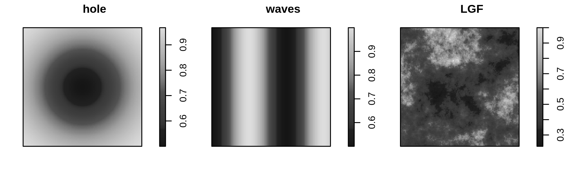
Figure 1: Plots of the ‘hole’, ‘waves’ and ‘LGF’ thinning profiles.

Simulations were carried out and analyzed using the R package spatstat, and a new package globalKinhom that implements the global $K$- and pair correlation function estimators using Monte-Carlo estimates of $\gamma$ as described in Section 5.3 (R Core Team, 2020; Baddeley, Rubak & Turner, 2015; Shaw, 2020). In most cases we set the precision of the Monte-Carlo estimates to $\alpha=.005$. When probability intervals and root integrated mean square error (RIMSE) values are shown, we use $\alpha=.001$ instead, where the more precise calculation produced slightly smaller RIMSE values. We also tested smaller values of $\alpha$ in a few particular cases, and did not observe any reduction in RIMSE values below $\alpha=.001$. We do not show simulation results for all scenarios since in many cases the different scenarios led to qualitatively similar conclusions.

To investigate our cross $K$ and cross pair correlation function estimators we generated simulations from a bivariate LGCP detailed in Section 6.2.

6.1 Estimation of $K$ and pair correlation functions

We initially compare the bias of global and local estimators of the $K$-function using in both cases kernel estimators of the intensity function obtained with a Gaussian kernel with bandwidth $\sigma$ chosen by the method of Cronie & van Lieshout (2018), as implemented in the spatstat procedure bw.CvL (CVL for convenience in the following). The selected bandwidths vary around .05 (see third column in Table 1), with slightly larger bandwidths for LGCP than for Poisson and DPP. For the global estimator we consider the isotropic estimator (5), since the pair correlation functions of the point processes tested here are all isotropic, as in the setting of Section 3.1.1, and the estimation of $\gamma^{\mathrm{iso}}$ is less computationally intensive than that of $\gamma$. We consider both the estimator (30) and the leave-out estimator (33) of the function $\gamma$. Similarly we also consider the local estimator using either the original kernel estimator (23) or the leave-out estimator (24) suggested in Baddeley, Møller & Waagepetersen (2000).

For better visualization of the simulation results we transform the $K$-function estimators into estimators of the so-called $\{L(r)-r\}$-function via the one-to-one transformation

$$L(r)-r=\sqrt{K(r)/\pi}-r.$$

We only show results in case of the waves intensity function with on average 400 simulated points, since the results for the other intensity functions and with on average 200 simulated points give the same qualitative picture.

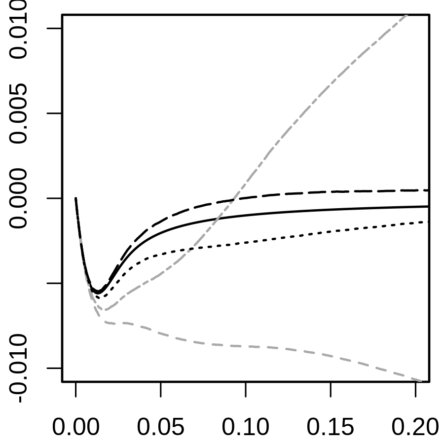
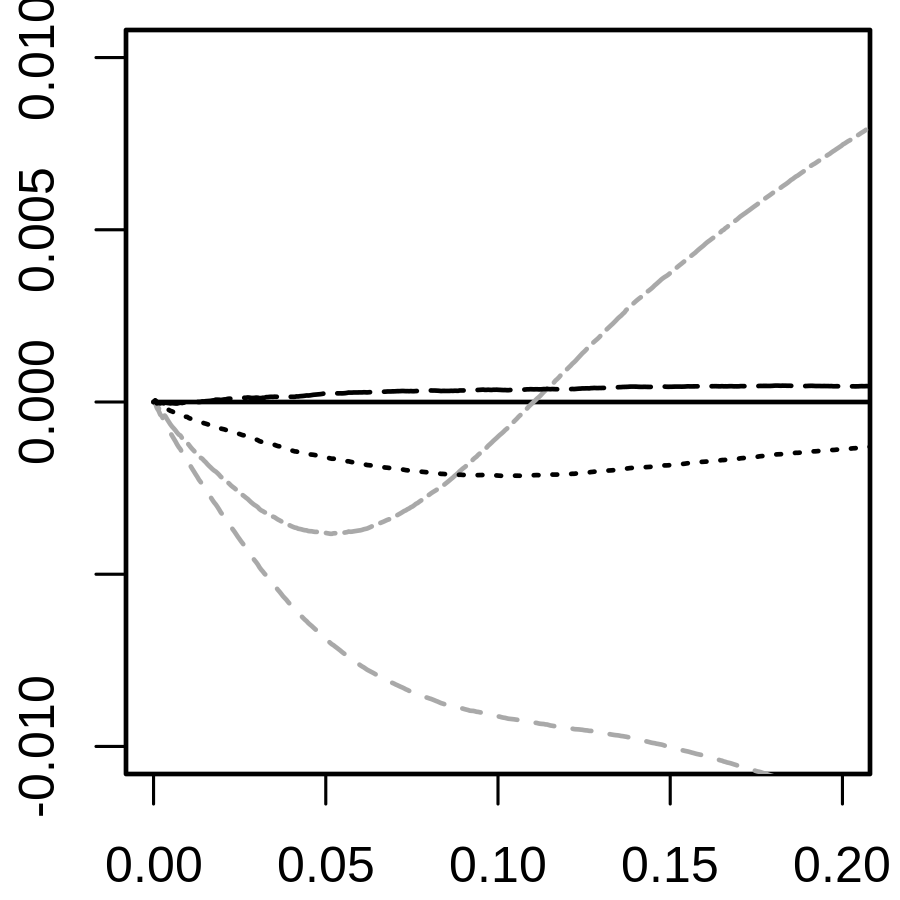
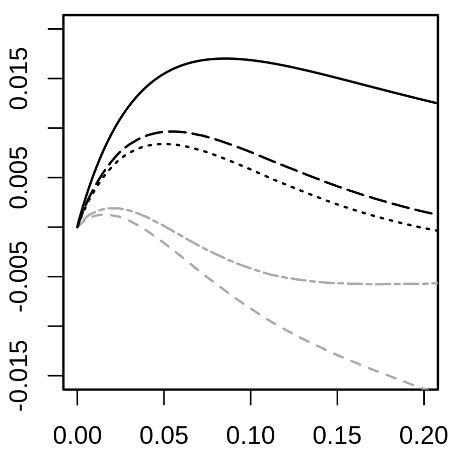
Figure 2: Averages of estimates of $L(r)-r$ obtained from simulations in case of the waves intensity function with 400 simulated points on average. Left to right: DPP, Poisson, LGCP. The estimates are obtained using $\hat{K}_{\mathrm{global}}^{\mathrm{iso}}$ with or without the leave-out approach (, , respectively) or $\hat{K}_{\mathrm{local}}$ with or without the leave-out approach (, , respectively) for kernel estimation of $\gamma$ or the intensity function. True values of $L(r)-r$ are shown for comparison ().

Figure 2 shows averages of the simulated estimates and it is obvious that the global estimators are much less biased than the local estimators. It is clearly advantageous to use the leave-out versions for the global estimator. The leave-out approach is also advantageous for the local estimator, at least for small distances $r$. The biases of the leave-out local estimator are as discussed in Section 5.1: strong negative bias at short distances due to the covariance of $\bar{\rho}(x)$ and $\bar{\rho}(y)$, and strong positive bias at large distances due to Jensen’s inequality $\text{E}(1/\bar{\rho}(x))>1/\text{E}(\bar{\rho}(x))$. The leave-out global estimator appears to be close to unbiased in case of DPP and Poisson but is too small on average in case of LGCP.

Table 1: Mean ($\pm$ st. dev.) of CVL and LCV bandwidths, for each type of spatial point process we considered. The expected number of points for each listed process is 400.

Interaction type	Intensity function	$\sigma_{\text{CVL}}$	$\sigma_{\text{LCV}}$
DPP	constant	0.046 (0.005)	0.63 (0.15)
	hole	0.045 (0.004)	0.33 (0.22)
	waves	0.048 (0.004)	0.28 (0.25)
	LGF	0.047 (0.005)	0.22 (0.16)
Poisson	constant	0.047 (0.006)	0.59 (0.21)
	hole	0.048 (0.007)	0.29 (0.23)
	waves	0.050 (0.006)	0.14 (0.11)
	LGF	0.050 (0.006)	0.17 (0.13)
LGCP	constant	0.066 (0.009)	0.040 (0.007)
	hole	0.064 (0.012)	0.044 (0.008)
	waves	0.071 (0.011)	0.042 (0.008)
	LGF	0.066 (0.011)	0.042 (0.007)

There exist a number of alternatives to the CVL approach to choosing the bandwidth for the kernel estimation. We therefore also investigate bias in the case where the bandwidth is selected using the likelihood cross validation (LCV) method implemented in the spatstat procedure bw.ppl. Results regarding the LCV selected bandwidths are summarized in the fourth column of Table 1. Comparison of the CVL and LCV results in Table 1 shows that the LCV approach tends to select considerably larger bandwidths $\sigma$ than the CVL method for the DPP and Poisson process, and somewhat smaller $\sigma$ for the LGCP.

Figure 3 compares averages of the global and local estimators using either of the two approaches to bandwidth selection and with leave-out in all cases. Again we show only results for the waves intensity function and expected number of points equal to 400.

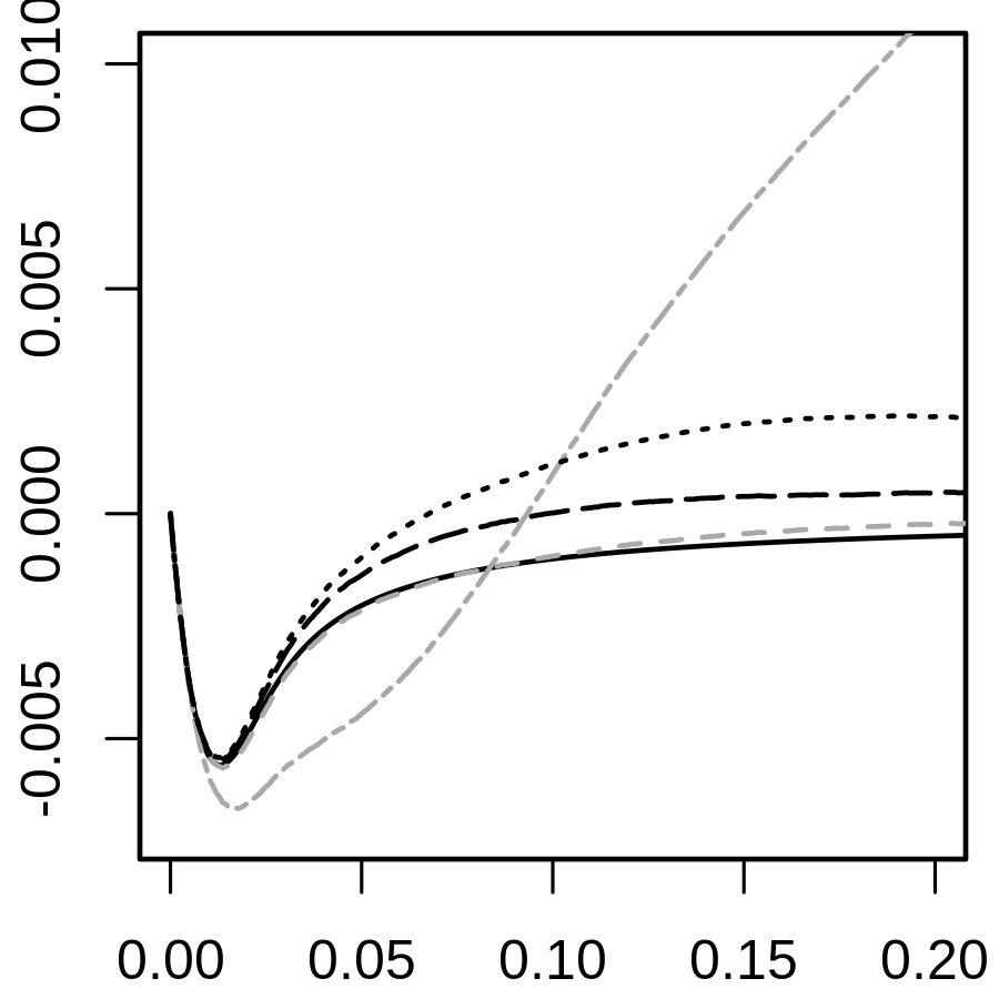
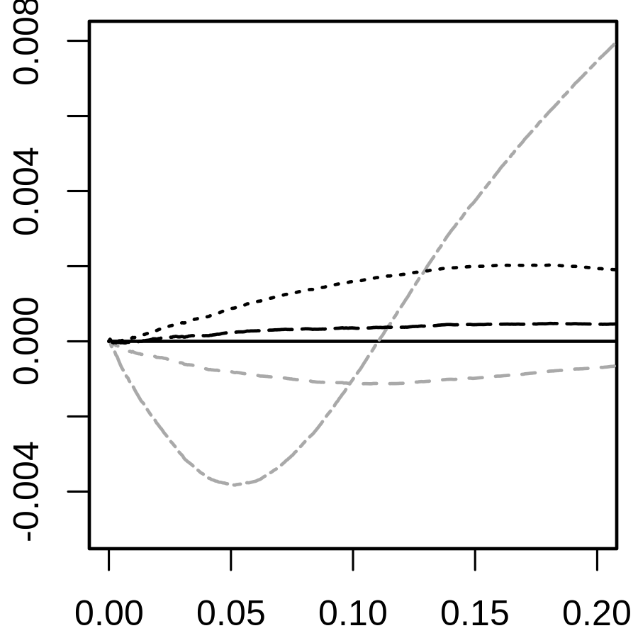
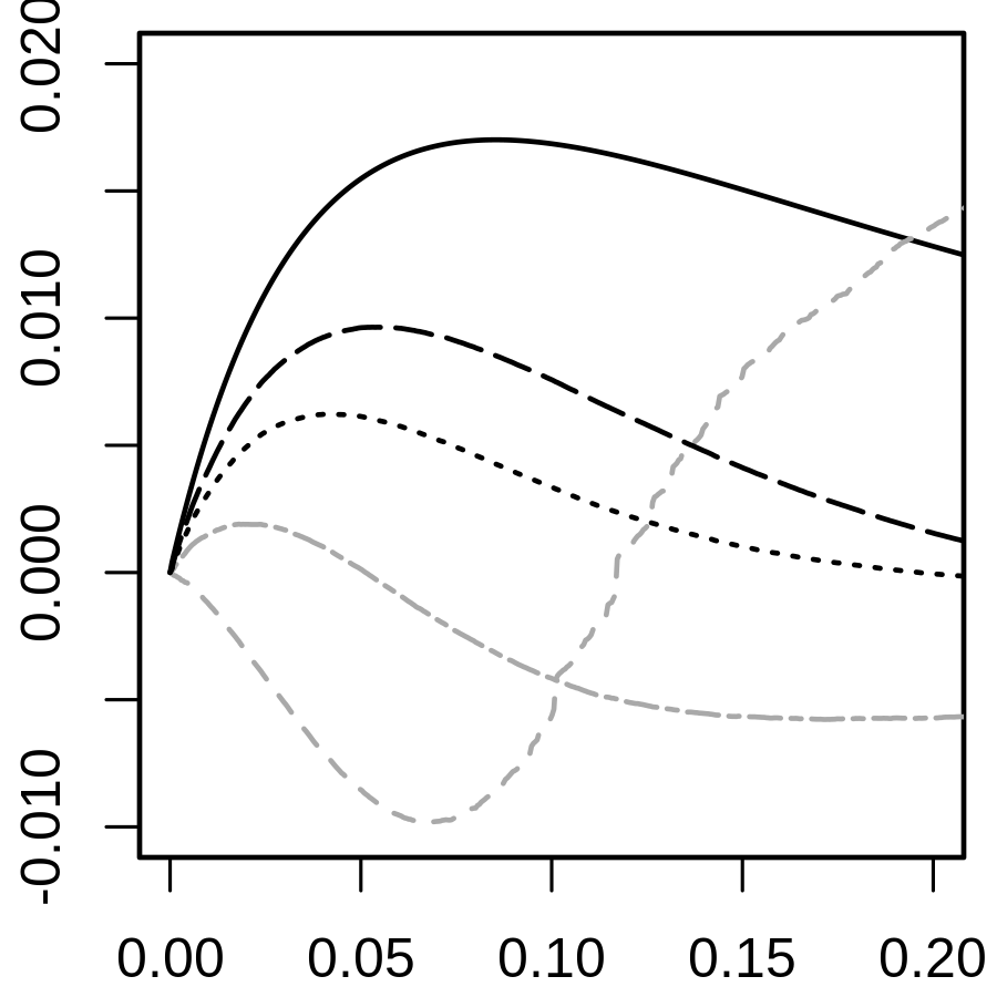
Figure 3: Averages of estimates of $L(r)-r$ obtained from simulations in case of the waves intensity function with 400 simulated points on average. Left to right: DPP, Poisson, LGCP. The estimates are obtained using the global ( CVL,  LCV) or local ( CVL,  LCV) estimators of the $K$-function with either CVL or LCV for selecting the bandwidth (in all cases the leave-out approach is used). True values of $L(r)-r$ are shown for comparison ().

The bias of the estimators is quite sensitive to the choice of bandwidth selection method. In case of DPP and Poisson, the global estimator using CVL and the local estimator using LCV perform similarly with the global estimator a bit more biased than the local for DPP and vice versa for Poisson. The global estimator performs slightly worse when combined with LCV than with CVL, likely due to the inherent biases of the kernel estimator $\bar{\rho}$, which become more pronounced as $\sigma$ increases. The local estimator with CVL is strongly biased for almost all $r$ considered. The improved performance with LCV is likely due to the reduced variances and covariances for $\bar{\rho}$ when a larger bandwidth is used. This also explains the strong bias of the local estimator with LCV for the LGCP, since $\sigma_{\mathrm{LCV}}$ is typically smaller than $\sigma_{\mathrm{CVL}}$ in that case. The global estimator for the LGCP has the smallest bias with the CVL method and has much less bias than the local estimator regardless of whether CVL or LCV is used. It is not surprising that the LGCP is the most challenging case for both the global and local estimators, since the random aggregation of the LGCP tends to be entangled with the variation in the intensity function.

We finally compare the sampling variability of the leave-out global estimator using CVL and the leave-out local estimator using LCV. Figure 4 shows 95% pointwise probability intervals and averages for the two estimators, again with 400 simulated points on average and the ‘waves’ intensity function, and Table 2 gives root integrated mean square error (RIMSE) values for the $K$-function estimators applied to each process, for each combination of CVL or LCV with the local or global leave-out estimator. Figure 4 indicates that the global estimator has smaller variance than the local estimator. This should also result in smaller mean square error for Poisson and LGCP where the bias is also smallest for the global estimator. For DPP the picture is not completely clear regarding mean square error since in this case the global estimator has larger bias than the local estimator. Table 2 gives more insight where a first observation is that the leave-out local estimator is very sensitive to the choice of bandwidth selection method with LCV performing much better than CVL for DPP and Poisson and vice versa for LGCP. The leave-out global estimator is much less sensitive to choice of bandwidth selection method. Best results in terms of RIMSE are obtained with the leave-out global estimator combined with CVL.

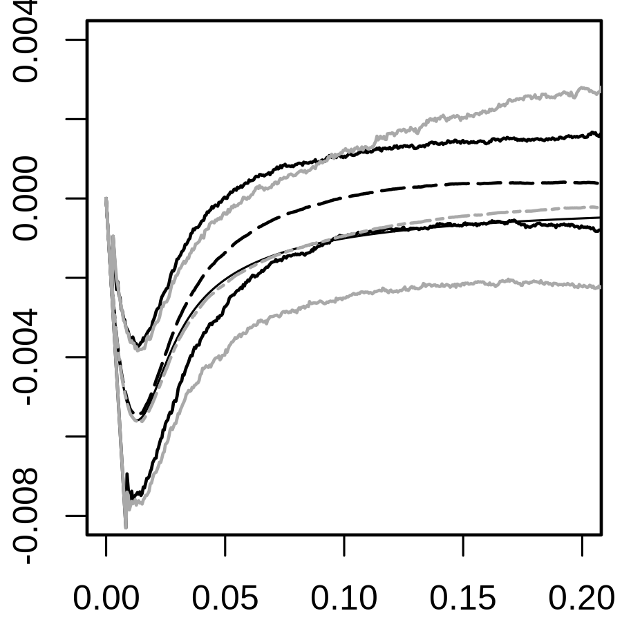
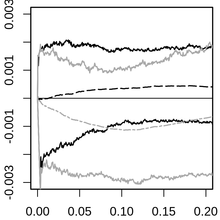
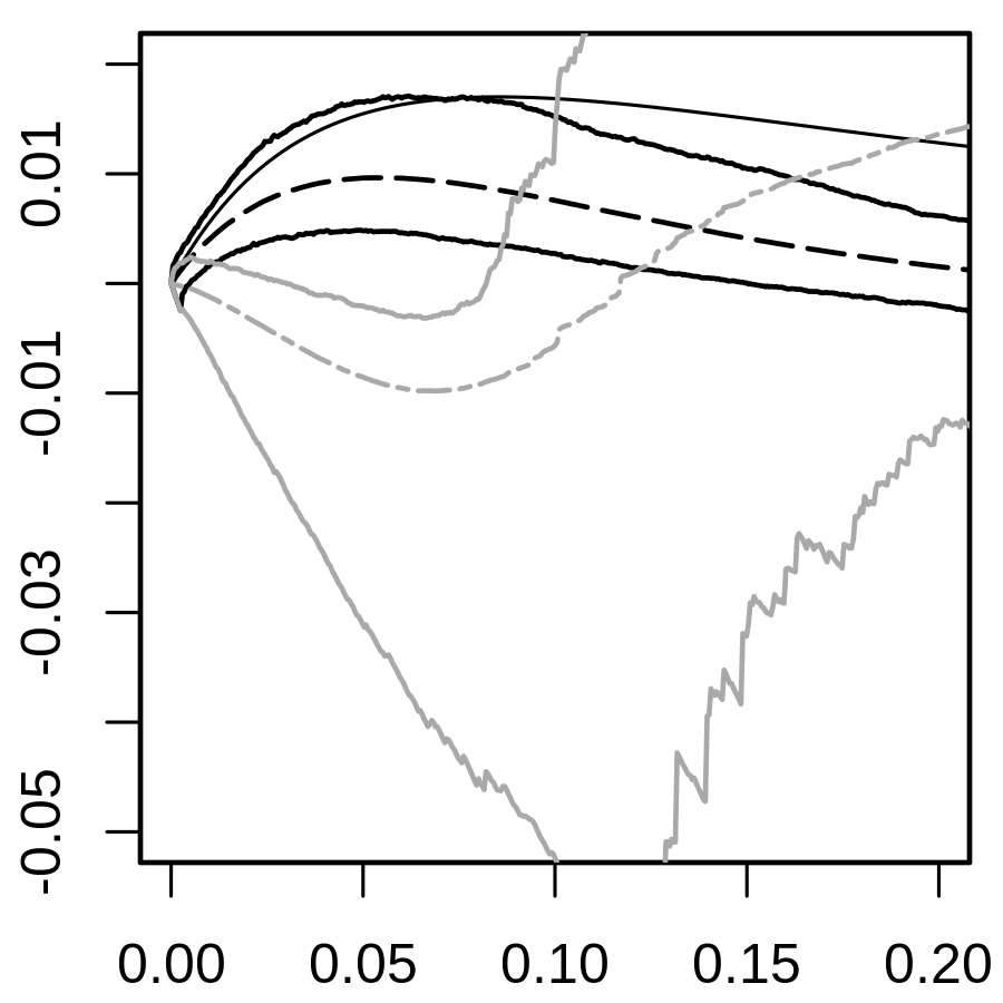
Figure 4: Averages and 95% pointwise probability intervals for estimates of $L(r)-r$ in case of the waves intensity function with 400 simulated points on average. Left to right: DPP, Poisson, LGCP. The estimators used are the leave-out global estimator using CVL () and the leave-out local estimator using LCV. (), with pointwise probability intervals shown in like shade. True values of $L(r)-r$ are also shown ().

Table 2: RIMSE $\times 10^{2}$ of local and global $K$-function estimators with CVL and LCV bandwidths.

		$\hat{K}_{\text{local}}$		$\hat{K}_{\text{global}}$
Interaction type	Intensity function	CVL	LCV	CVL	LCV
DPP	flat	0.59	0.069	0.029	0.060
	hole	0.64	0.107	0.031	0.128
	waves	0.60	0.052	0.049	0.121
	LGF	0.59	0.060	0.050	0.110
Poisson	flat	0.45	0.083	0.028	0.069
	hole	0.45	0.120	0.034	0.103
	waves	0.40	0.061	0.037	0.093
	LGF	0.37	0.087	0.050	0.089
LGCP	flat	0.89	0.999	0.573	0.628
	hole	0.87	1.554	0.576	0.636
	waves	0.89	1.146	0.528	0.613
	LGF	0.90	1.506	0.542	0.625

Figure 5 shows averages of leave-out global and local estimators of the isotropic pair correlation function using either CVL or LCV in case of the wave intensity with 400 points on average. Once again, local estimators are most strongly biased with the bandwidth selection method that produces the smaller bandwidth: CVL for the DPP and Poisson processes, and LCV for the LGCP. The bias is small to moderate for the global estimators with largest bias in case of LGCP. For the DPP and Poisson case positive bias of the local and global estimator occurs for very small distances.

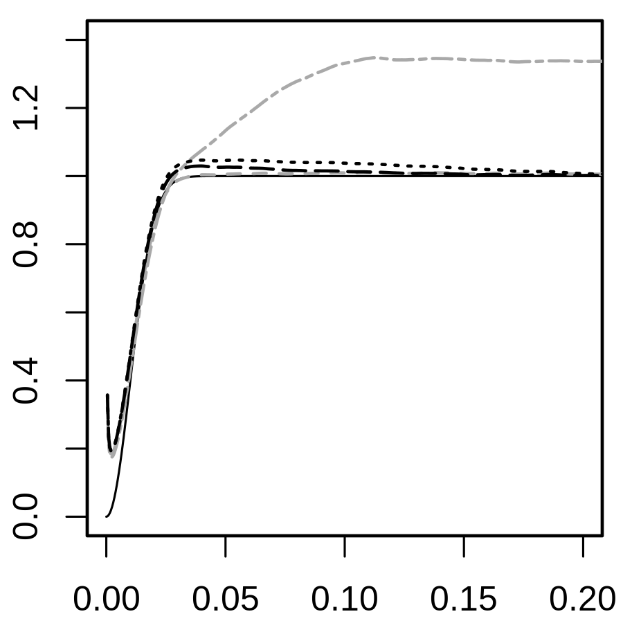
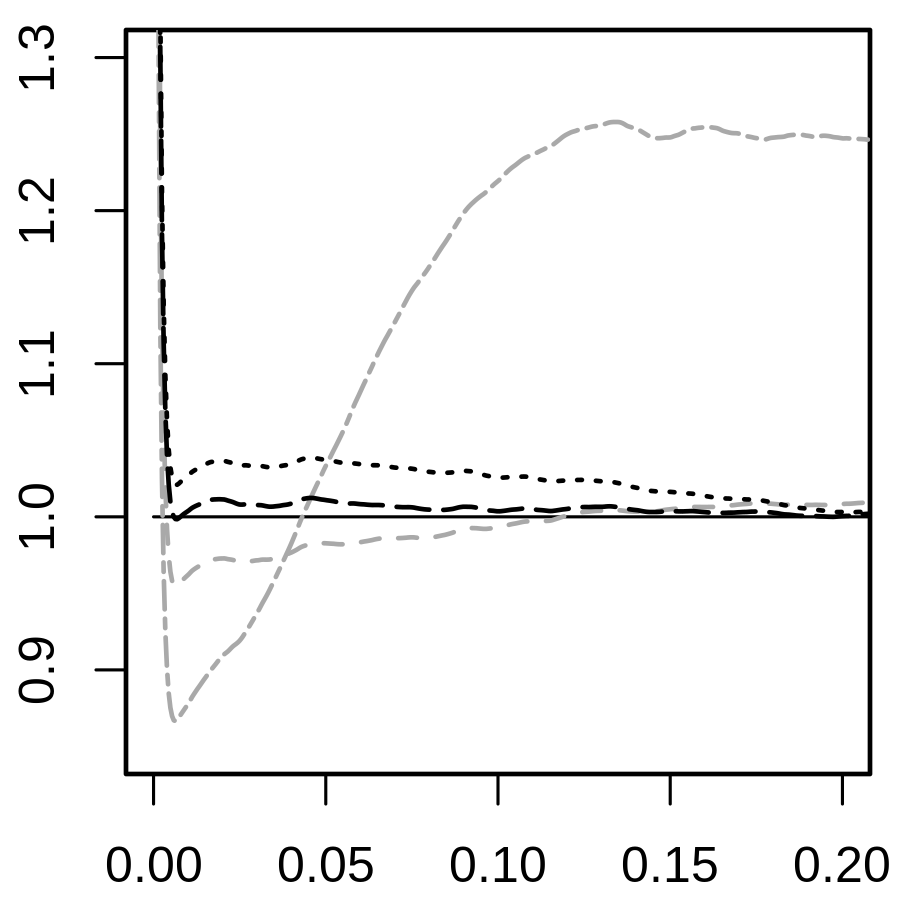
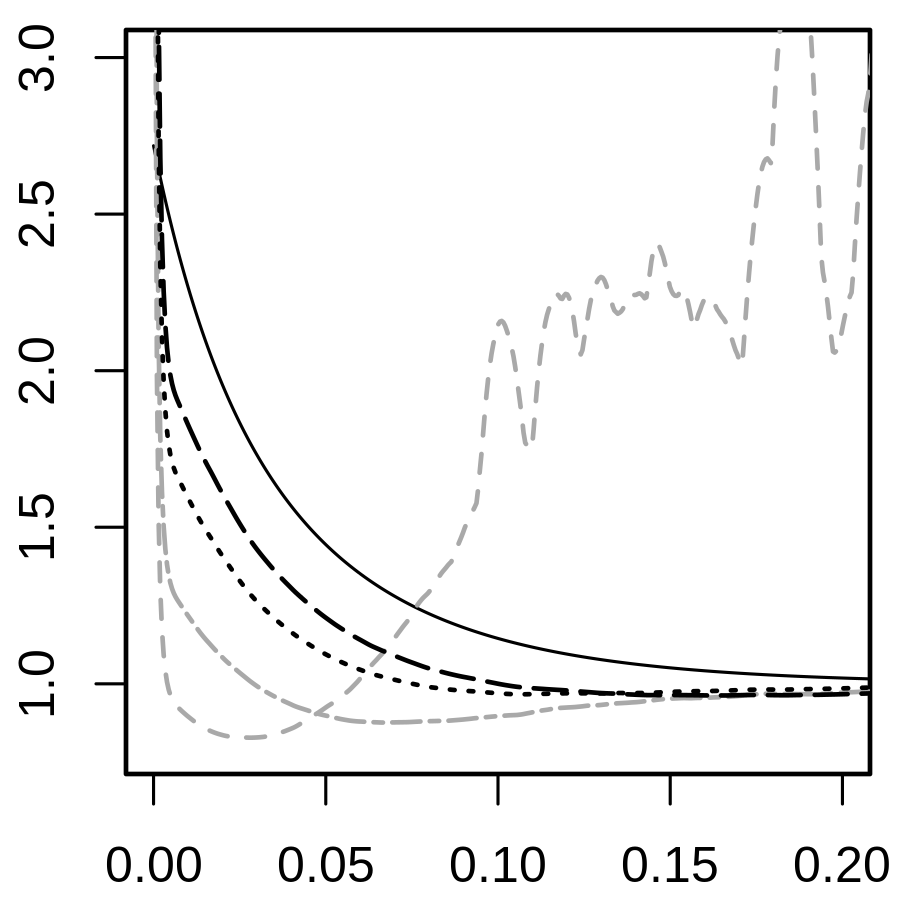
Figure 5: Averages of estimates of $g_{1}(r)$ obtained from simulations in case of the waves intensity function with 400 simulated points on average. Left to right: DPP, Poisson, LGCP. The estimates are obtained using the global ( CVL,  LCV) or local ( CVL,  LCV) estimators of the pair correlation function with either CVL or LCV bandwidth selection. (In each case, the leave-out approach is used.) True values of $g(r)$ are shown for comparison ().

6.2 Estimation of cross $K$ and cross pair correlation functions

To investigate the cross $K$ and cross pair correlation function estimators, we simulated 100 bivariate point patterns for each model of a bivariate point process $(X_{1},X_{2})$, where either $X_{1}$ and $X_{2}$ are independent or display segregation or co-clustering. Processes that were chosen for plotting were simulated an additional 1000 times. Inhomogeneous intensity functions were subsequently obtained using independent thinning of stationary bivariate point processes, where the two point processes have the same intensity, and the constant, ‘hole’, and ‘waves’ retention probabilities $p$ as described in connection to Figure 1 were used. This implies $\rho_{1}(x)=\rho_{2}(x)$ for $x\in[0,1]^{2}$ (we did not investigate any scenarios where $\rho_{1}\neq\rho_{2}$).

In the case of independence, $X_{1}$ and $X_{2}$ are independent Poisson processes. For the dependent cases, we considered a bivariate LGCP. Specifically, for $i=1,2$, $X_{i}$ has random intensity function

$$\Lambda_{i}(u)=p(u)\exp\{\mu_{i}+\alpha_{i}Y(u)+\beta U_{i}(u)\},\qquad i=1,2,$$

where $Y$, $U_{1}$, and $U_{2}$ are independent zero-mean unit-variance Gaussian random fields with isotropic exponential correlation functions given by $\exp(-r/\phi)$ and $\exp(-r/\psi_{i})$ ($r\geq 0$), $i=1,2$, respectively, and where $\mu_{i}\in\mathbb{R}$, $\alpha_{i}\in\mathbb{R}$, and $\beta>0$ are parameters. This means that $X_{1}$ and $X_{2}$ conditioned on $(\Lambda_{1},\Lambda_{2})$ are independent Poisson processes with intensity functions $\Lambda_{1}$ and $\Lambda_{2}$, respectively. The (cross) pair correlation functions for this class of bivariate LGCP are isotropic, where the pair correlation function of $X_{i}$ is given by

$$g^{\mathrm{iso}}_{i}(r)=\exp\{\alpha_{i}^{2}\exp(-r/\phi)+\beta\exp(-r/\psi_{i})\},\qquad i=1,2,$$

and the cross pair correlation function of $(X_{1},X_{2})$ is given by

$$c^{\mathrm{iso}}(r)=\exp\{\alpha_{1}\alpha_{2}\exp(-r/\phi)\}.$$

Note that $c^{\mathrm{iso}}<1$ if $\alpha_{1}\alpha_{2}<0$ (the case of segregation between $X_{1}$ and $X_{2}$), and $c^{\mathrm{iso}}>1$ if $\alpha_{1}\alpha_{2}>0$ (the case of co-clustering between $X_{1}$ and $X_{2}$). For the segregated processes, we chose $\alpha_{1}=-\alpha_{2}=1$, $\phi=.03$, $\beta=.25$, $\psi_{1}=.02$, and $\psi_{2}=.01$. For the co-clustered case, we used $\alpha_{1}=\alpha_{2}=1$ and the other parameters as for the segregated case. With these choices, the cross correlation functions become

$$c^{\mathrm{iso}}_{\mathrm{segr}}(r)=\exp\{-\exp(-r/.03)\}$$

for the segregation case and

$$c^{\mathrm{iso}}_{\mathrm{cluster}}(r)=\exp\{\exp(-r/.03)\}$$

for the co-clustered case. Finally, we adjusted $\mu_{1}$ and $\mu_{2}$ so that the expected number of points after independent thinning is 200 or 400.

For the global estimator of $K_{12}$, we consider again the isotropic estimator (13), since in each case the cross pair correlation function is isotropic, and estimation of $\gamma_{12}^{\mathrm{iso}}(r)$ is less computationally intensive than that of $\gamma_{12}(h)$. For the local estimator we consider the estimator (11), with $\rho_{i}$ estimated by the leave-out kernel estimator $\bar{\rho}$ from (24). Similar to the $\{L(r)-r\}$-function used above, we transform the $K_{12}$-function estimators into estimators of the $\{L_{12}(r)-r\}$-function, by the one-to-one transformation

$$L_{12}(r)-r=\sqrt{K_{12}(r)/\pi}-r.$$

Figure 6 shows averages of estimators of $L_{12}(r)-r$ in case of the waves intensity and expected number of points equal to 400. The bandwidth is selected using the CVL or LCV procedure applied to $X_{1}$. Table 3 gives selected bandwidth values for the pairs of spatial point processes we considered. The results are similar to the one point process case. Both the segregated and co-clustered LGCP typically yield $\sigma_{\mathrm{LCV}}<\sigma_{\mathrm{CVL}}$ while the opposite is true for the Poisson case. Further, the local estimators are strongly biased, and the bias increases as the bandwidth $\sigma$ decreases: in the case of segregation and co-clustering, the local estimators are better with CVL, while LCV is better in the case of independence. Note also that the negative bias that is observed at small distances $r$ for $\hat{K}_{\mathrm{local}}$ is absent here as predicted in the discussion in Section 5.1. The bias for the global estimator with CVL is smaller than for the best local estimators in each case.

Table 3: Mean ($\pm$ st. dev.) of CVL and LCV selected bandwidths for the simulated two point process cases. Expected number of points is 400 for each listed process.

Interaction type	Intensity function	$\sigma_{\text{CVL}}$	$\sigma_{\text{LCV}}$
Segregated	constant	0.063 (0.008)	0.038 (0.006)
	hole	0.062 (0.009)	0.039 (0.008)
	waves	0.064 (0.010)	0.040 (0.008)
Poisson	constant	0.048 (0.006)	0.60 (0.19)
	hole	0.048 (0.006)	0.28 (0.22)
	waves	0.051 (0.006)	0.19 (0.20)
Co-clustered	constant	0.062 (0.008)	0.040 (0.008)
	hole	0.060 (0.009)	0.040 (0.007)
	waves	0.064 (0.011)	0.040 (0.009)

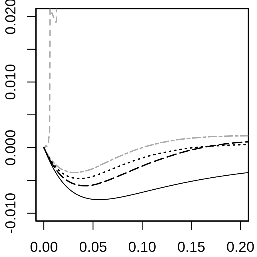
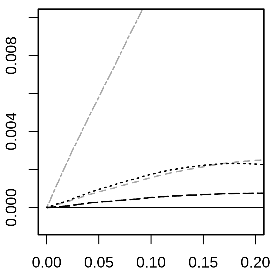
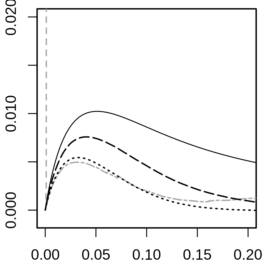
Figure 6: Averages of estimates of cross-$L(r)-r$ in case of the waves intensity function with 400 simulated points on average. Left to right: segregation, independence, co-clustering. The estimators used are the standard global ( CVL,  LCV) and local ( CVL,  LCV) leave-out estimators of $K_{12}$ combined with the CVL and LCV methods for the bandwidth selection. True values of $L_{12}(r)-r$ are shown for comparison ().

To compare sampling variability for the estimators of the cross $K$-function, we show pointwise 95% probability intervals for estimated $L_{12}(r)-r$ in Figure 7. The bandwidth selection method that produces the least bias in each case is shown. Table 4 shows root integrated mean square error of the estimators of $K_{12}$. In every case, the best global estimator has smaller integrated mean square error than the best local estimator, as expected from the considerations of Section 3.1.2.

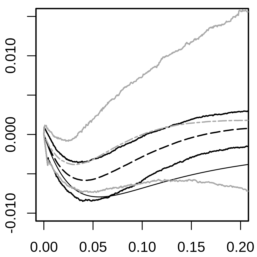
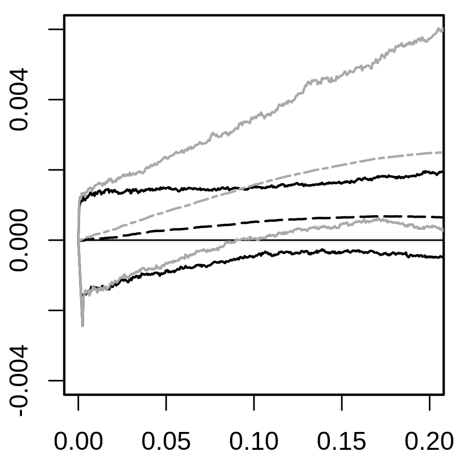
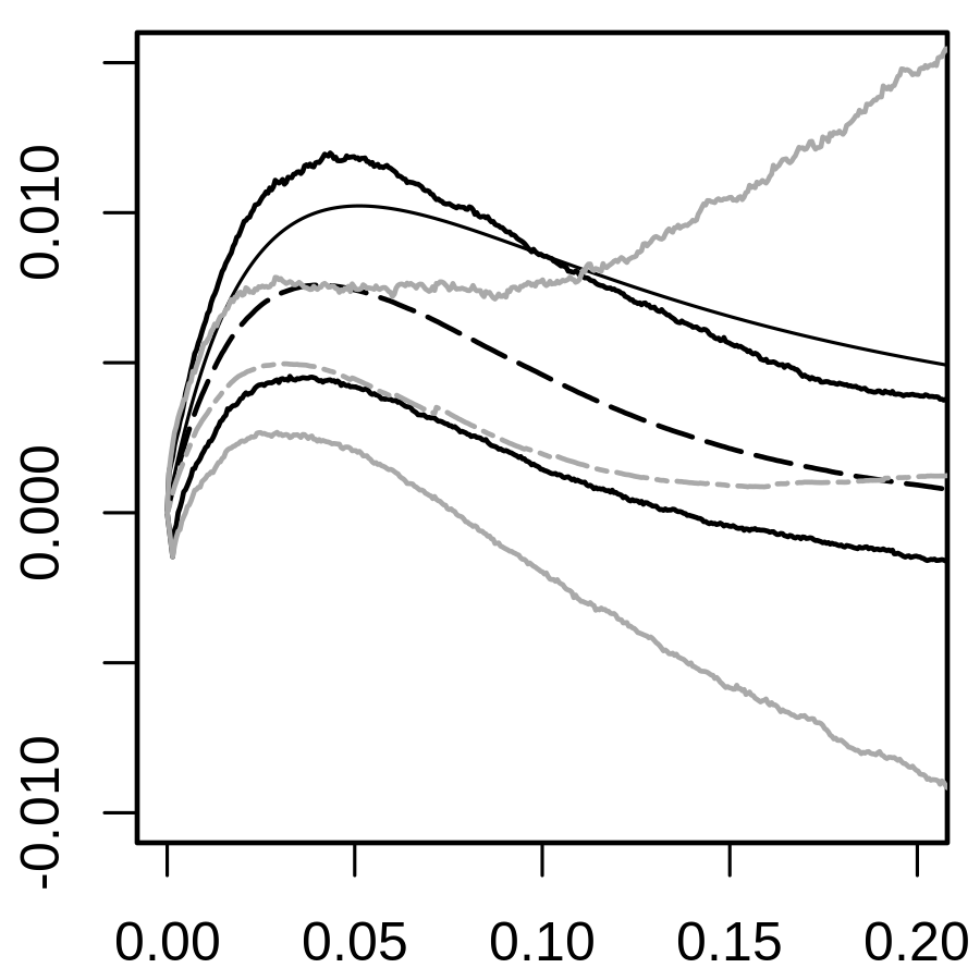
Figure 7: Averages and 95% pointwise probability intervals for estimates of $L_{12}(r)-r$ in case of the waves intensity function with 400 simulated points on average. Left to right: segregation, independence, co-clustering. The estimators used are the leave-out global estimator () and the leave-out local estimator (), with pointwise probability intervals shown in like shade. In each case, the bandwidth selection method was chosen to produce the least bias: LCV for the local estimator on the independent process, and CVL for all the other cases. True values of $L_{12}(r)-r$ are also shown ().

Table 4: Root integrated mean squared errors $\times 10^{2}$ of local and global $K_{12}$-function estimators with CVL and LCV bandwidths.

		$\hat{K}_{12,\text{local}}$		$\hat{K}_{12,\text{global}}$
Interaction type	Intensity function	CVL	LCV	CVL	LCV
Segregated	flat	0.65	390.125	0.161	0.181
	hole	0.69	4.574	0.171	0.185
	waves	0.64	270.633	0.208	0.201
Independent	flat	1.03	0.066	0.024	0.049
	hole	1.09	0.112	0.026	0.109
	waves	0.95	0.191	0.037	0.104
Co-clustered	flat	0.92	18.783	0.234	0.262
	hole	0.97	3.510	0.239	0.265
	waves	0.92	5.238	0.195	0.244

For the estimation of the cross pair correlation functions, the conclusions are similar to those for the cross $K$-functions, see Figure 8. The average of the global estimator is quite close to the true cross pair correlation function, while the local estimator is strongly biased. Note that $\hat{c}_{\mathrm{local}}^{\mathrm{LCV}}$ is missing for the segregated and co-clustered processes, because the average values of that estimator were extremely large.

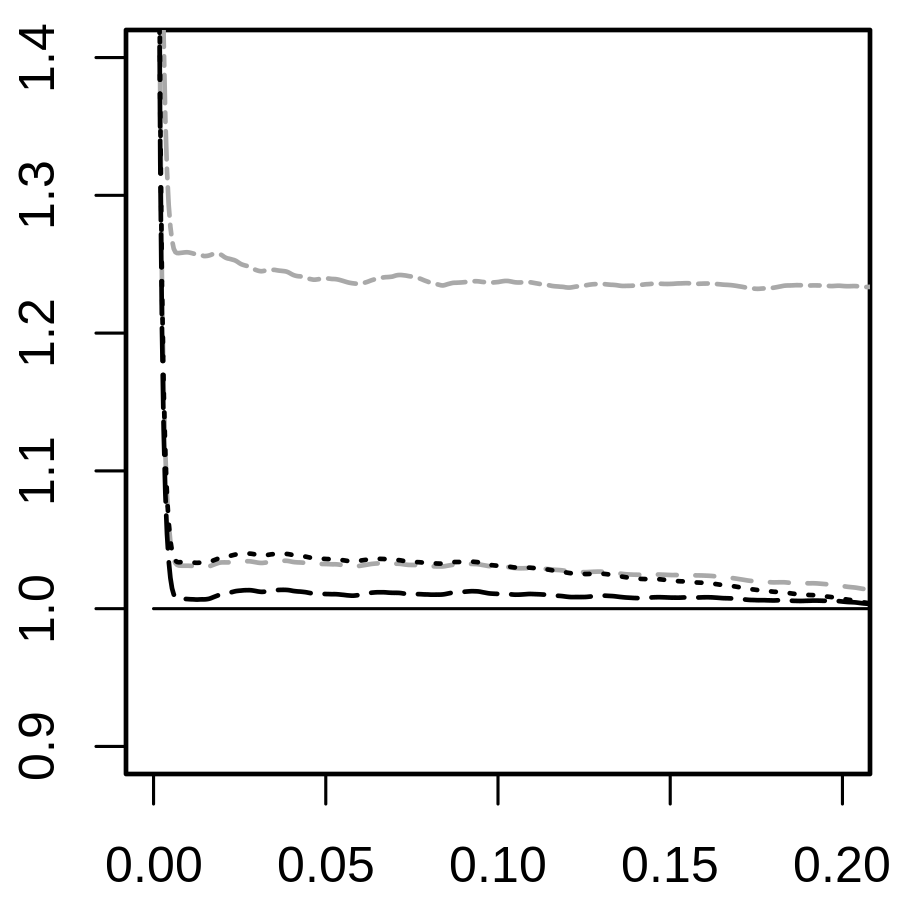
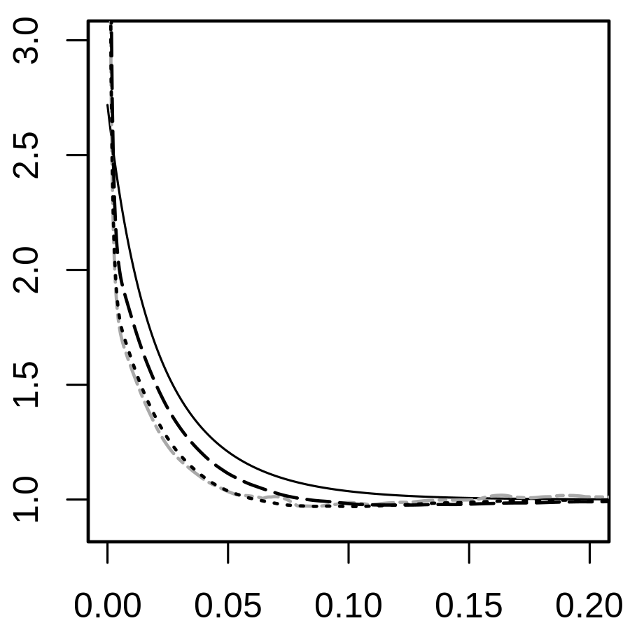
Figure 8: Averages of estimates of $c(r)$ in case of the waves intensity function with 400 simulated points on average. Left to right: segregation, independence, co-clustering. The estimators used are the leave-out global ( CVL,  LCV) and local ( CVL,  LCV) estimators combined with the CVL and LCV methods for bandwidth selection. True values of $L_{12}(r)-r$ are shown for comparison ().

6.3 Estimation of $K$-function using a parametric estimate for $\rho$

Returning to the setting of a single point process $X$ as in the beginning of Section 6, we also consider the case of a parametric model where the intensity $\alpha>0$ of the underlying stationary point process (that is, before thinning) is unknown but the retention probability function $p$ that was used to thin the point process is known. Then a simple parametric estimator for $\rho$ is given by

$$\hat{\rho}_{p}(x)=Np(x)\big{/}\int_{W}p(x)\,\mathrm{d}x,$$ (37)

where $N$ is the number of points in $X\cap W$. We apply this intensity estimator to $\hat{K}_{\text{local}}$ and $\hat{K}_{\text{global}}$ for $1000$ realizations of each interaction type, with the ‘waves’ intensity function and expected number of points equal to 400. In addition, we generate $1000$ simulations for each interaction type with a new thinning profile, ‘deep waves’, given by

$$p_{\text{deep}}(x,y)=1-.9\cos^{2}(5x),\qquad(x,y)\in[0,1]^{2}.$$

The deep waves profile is similar to the waves profile, but with much more extreme intensity variations.

Pointwise probability intervals for estimates of $L(r)-r$ are shown in Figure 9, and root integrated mean square error for estimates of $K$ are given in Table 5. We observe that in all cases the error of the global estimator is comparable to or better than the corresponding local estimator. For the ‘waves’ intensity function, the difference is small. Both estimators have larger error when applied to the patterns with the ‘deep waves’ intensity function. However, the performance of the local estimator degrades much more strongly, reflecting the fact that regions of low intensity are weighted more heavily in $\hat{K}_{\text{local}}$ than in $\hat{K}_{\text{global}}$, as discussed in Section 3.1.2. The LGCP yielded the largest errors with the parametric intensity estimates, similar to our observations with the kernel-based intensity estimates. We also note that for the DPP and the Poisson process, using the parametric estimates for the ‘waves’ intensity function results in higher integrated mean square error than for the kernel-based estimates (Table 2). We believe this is because the kernel-based estimates of $\rho$ are adapted to the random local fluctuations of the point processes, similar to how homogeneous $K$-function estimates have lower variance when using estimated intensity than true intensity. However, for the LGCP, best results are obtained with the parametric estimates, which presumably are less prone to confounding of random clustering with variations in the intensity function.

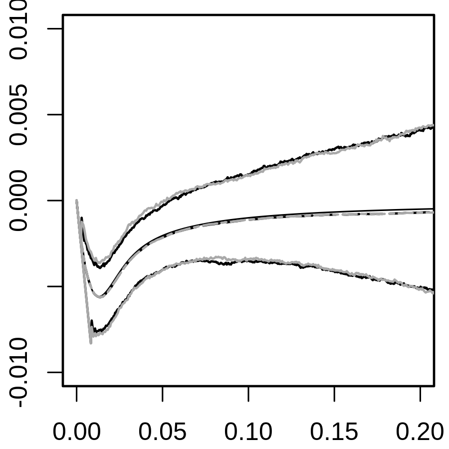
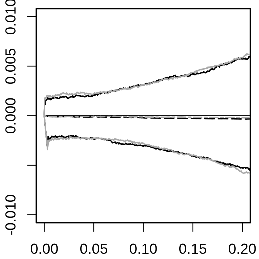
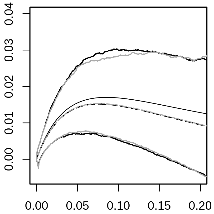
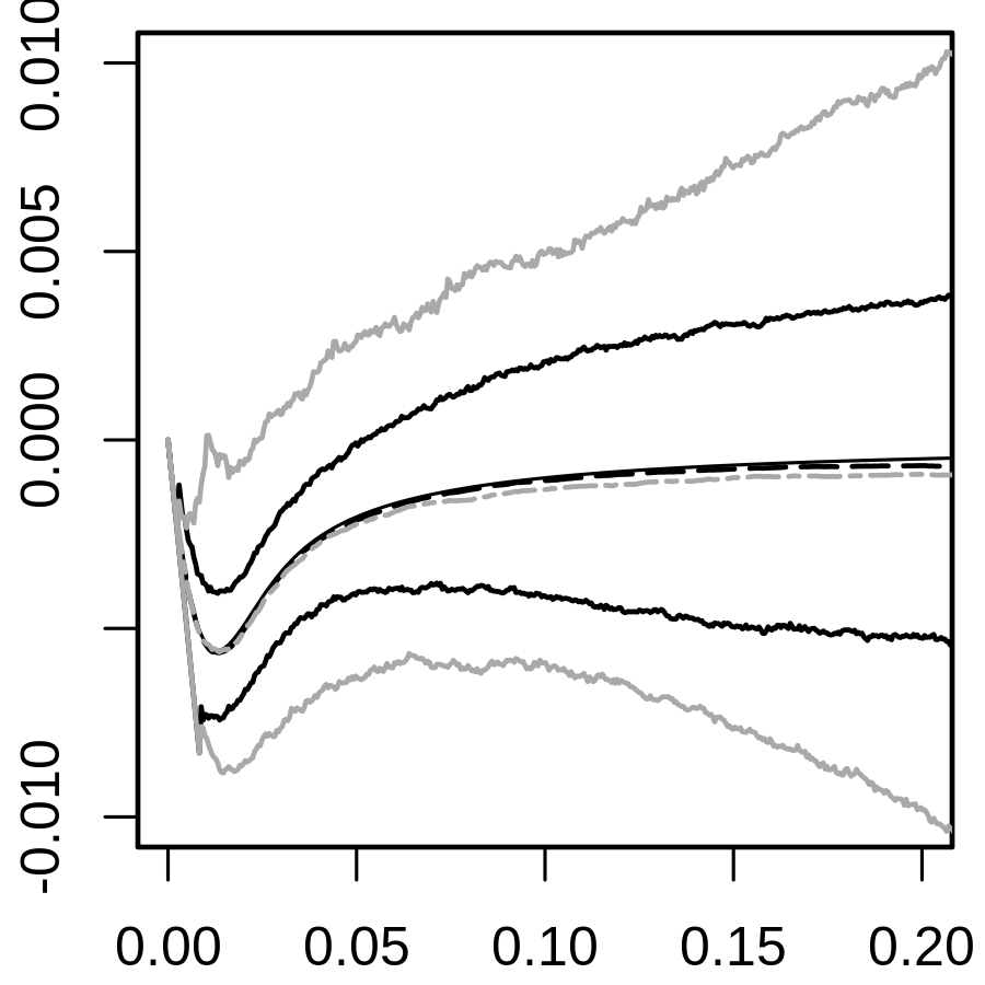
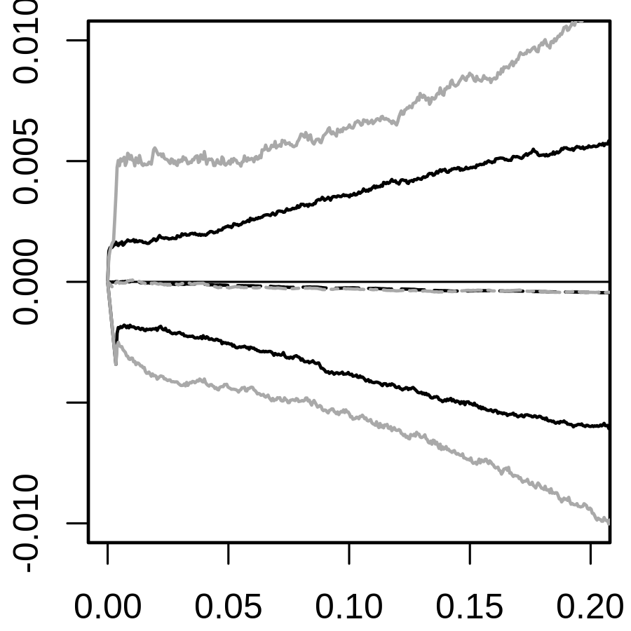
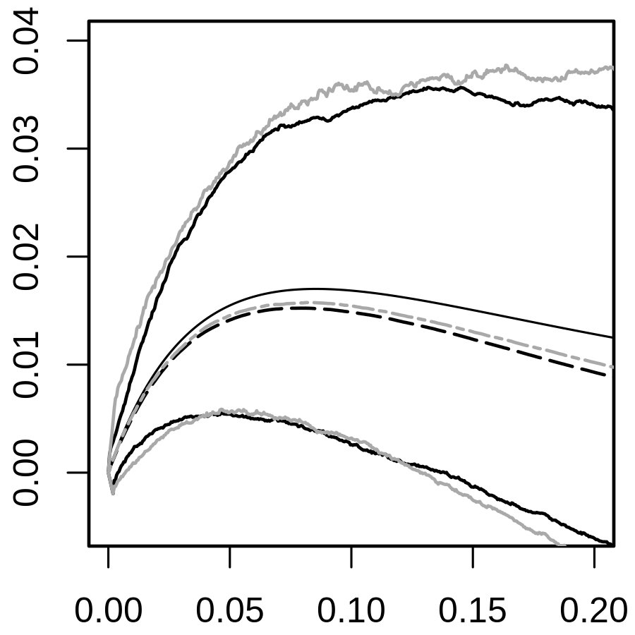
Figure 9: Averages and 95% pointwise probability intervals for estimates of $L(r)-r$ in case of the ‘waves’ (top row) or ‘deep waves’ (bottom row) intensity function with 400 simulated points on average. Left to right: DPP, Poisson, LGCP. The estimators used are the global () and local () estimators using the parametric intensity estimator (37). Pointwise probability intervals are shown in like shade. True values of $L(r)-r$ are also shown ().

Table 5: Root integrated mean squared errors $\times 10^{2}$ of local and global $K$-function estimators with parametric intensity estimator, applied to point processes with intensity function ‘waves’ or ‘deep waves’.

Interaction type	Intensity function	$\hat{K}_{\text{local}}$	$\hat{K}_{\text{global}}$
DPP	waves	.111	.102
	deep waves	.227	.103
Poisson	waves	.132	.122
	deep waves	.239	.133
LGCP	waves	.416	.417
	deep waves	.601	.516

7 Extensions

The same sort of analysis as in Sections 3-4 could be applied to point processes defined on a non-empty manifold on which a group acts transitively (a so-called homogeneous space), where the space is equipped with a reference measure which is invariant under the group action. In this paper, the space was $\mathbb{R}^{d}$, the group action was given by translations, and the reference measure was Lebesgue measure. For example, instead we could consider the space to be a $d$-dimensional sphere, with the group action given by rotations and where the reference measure is the corresponding $d$-dimensional surface measure. Then the global and local estimators considered in this paper are simply modified to the case of the sphere by replacing Lebesgue with surface measure and using appropriate edge correction factors as defined in Lawrence et al. (2016). Similarly, our global estimators could also be extended to the case of spatio-temporal point processes, as in Gabriel & Diggle (2009) and Møller & Ghorbani (2012).

8 Conclusion

According to our simulation studies, our new global estimators outperform the existing local estimators in terms of bias and mean integrated squared error when kernel or parametric estimators are used for the intensity function. The kernel intensity function estimators depend strongly on the choice of bandwidth and we considered two different data-driven approaches, CVL and LCV, to bandwidth selection. In our simulation studies the two approaches gave similar selected bandwidths in the LGCP case but very different results in case of Poisson and DPP. This has a considerable impact on the $K$- and pair correlation function estimators but the global estimators appear to be much less sensitive to the choice of bandwidth selection method than the local estimators. The simulation studies with parametric estimates of the intensity function, along with the theory of Section 3.1.2, indicate that the global estimators are also much less sensitive to regions of especially low intensity. The improved statistical efficiency comes at a considerable extra computational cost. Therefore, we especially recommend the global estimators for situations where intensity variations are large and where computational speed is not a primary concern.

References

- Baddeley, Rubak & Turner (2015) Baddeley, A., Rubak, E. & Turner, R. (2015). Spatial Point Patterns: Methodology and Applications with R. London: Chapman & Hall/CRC Press.