Deep Learning for Radio Resource Allocation with Diverse Quality-of-Service Requirements in 5G

Abstract

To accommodate diverse Quality-of-Service (QoS) requirements in 5th generation cellular networks, base stations need real-time optimization of radio resources in time-varying network conditions. This brings high computing overheads and long processing delays. In this work, we develop a deep learning framework to approximate the optimal resource allocation policy that minimizes the total power consumption of a base station by optimizing bandwidth and transmit power allocation. We find that a fully-connected neural network (NN) cannot fully guarantee the QoS requirements due to the approximation errors and quantization errors of the numbers of subcarriers. To tackle this problem, we propose a cascaded structure of NNs, where the first NN approximates the optimal bandwidth allocation, and the second NN outputs the transmit power required to satisfy the QoS requirement with given bandwidth allocation. Considering that the distribution of wireless channels and the types of services in the wireless networks are non-stationary, we apply deep transfer learning to update NNs in non-stationary wireless networks. Simulation results validate that the cascaded NNs outperform the fully connected NN in terms of QoS guarantee. In addition, deep transfer learning can reduce the number of training samples required to train the NNs remarkably.

I Introduction

I-A Background

The 5th Generation (5G) cellular networks are expected to support various emerging applications with diverse Quality-of-Service (QoS) requirements, such as enhanced mobile broadband services, massive machine-type communications, and Ultra-Reliable and Low-Latency Communications (URLLC) [2]. To guarantee the QoS requirements of different types of services, existing optimization algorithms for radio resource allocation are designed to maximize spectrum efficiency or energy efficiency by optimizing scarce radio resources, such as time-frequency resource blocks and transmit power, subject to QoS constraints [3, 4, 5, 6, 7, 8, 9].

There are two major challenges for implementing existing optimization algorithms in practical 5G networks. First, QoS constraints of some services, such as delay-sensitive and URLLC services, may not have closed-form expressions. To execute an optimization algorithm, the system needs to evaluate the QoS achieved by a certain policy via extensive simulations or experiments, and thus suffers from long processing delay [9, 10]. Second, even if the closed-form expressions of QoS constraints can be obtained in some scenarios, the optimization problems are non-convex in general [10, 11, 8]. The system also needs to update resource allocation by solving non-convex problems to accommodate the time-varying channel and traffic conditions, leading to very high computing overhead. Even for some convex optimization problems that can be solved by well-developed methods, like the interior-point method, the computing complexity is still too high to be implemented in real time [12].

Deep learning is a promising approach to find the optimal resource allocation in real time [13, 14, 15, 16, 17]. The basic idea is to use an artificial Neural Network (NN) to approximate the optimal resource allocation policy that maps the system states to the optimal resource allocation. The system first trains the NN off-line with a large number of labeled samples. After the training phase, the optimal resource allocation can be obtained from the output of the NN for any given input. According to the Universal Approximation Theory, if the optimal policy is a deterministic and continuous function, then the approximation errors approach to zero as the number of neurons goes to infinite [18].

It is worth noting that the application of deep learning in wireless networks is not straightforward. For some discrete optimization variables, such as the number of subcarriers, antennas and the user association decisions, the approximation of the NN can be inaccurate due to the quantization of these discrete variables. As a result, the solution obtained from the NN cannot fully guarantee the QoS requirements of different types of services. In addition, deep learning requires a large number of labeled training samples. To obtain labeled training samples, we should first design an optimization algorithm to solve the formulated optimization problem. Even if a large number of labeled training samples are obtained with the optimization algorithm, the pre-trained NN is not accurate when the wireless network is non-stationary. For example, the distribution of wireless channels and the types of services in the network may vary. These non-stationary parameters that are not included in the input of the NN are referred to as hidden variables [19]. During the training phase, we assume that the hidden variables are fixed. However, in practical systems, these hidden variables drift over time. As discussed in [19], the dynamic hidden variables can be pernicious in deep learning.

I-B Related Works

Improving resource utilization efficiency for different kinds of services has been extensively studied in the literature. For delay-tolerant services, the QoS requirement is formulated as an average data rate requirement in Orthogonal Frequency Division Multiple Access (OFDMA) systems [20], where the subcarrier and transmit power allocation and antenna configuration were optimized. To guarantee the queueing delay bound and the delay bound violation probability of real-time services, effective capacity was adopted in [21, 22] to optimize bandwidth allocation and power control schemes. In URLLC, to reduce transmission delay, the blocklength of channel codes is short, and the fundamental relation between decoding error probability and blocklength was derived in [23]. This relation was used to optimize resource allocation for short packet transmissions in URLLC [7, 24, 8]. For most of these problems, the QoS constraints do not have closed-form expressions and the optimization algorithms cannot be executed in a real-time manner.

Approximating optimal resource allocation policies with NNs has been investigated in [13, 25, 14]. The authors of [13] proved that an iterative algorithm for power control in wireless networks can be accurately approximated by a Fully-connected Neural Network (FNN). In [25] and [17], convolutional neural networks were used to approximate the power control policy and the content delivery policy, respectively. To improve energy efficiency, [14] proposed an online deep learning approach to approximate the energy-efficient power control scheme obtained from the monotonic fractional programming framework in [26]. When the optimal optimization algorithm is not available, unsupervised deep learning was applied in [27, 28], where the parameters of a NN are trained to satisfy the Karush-Kuhn-Tucker (KKT) conditions of the optimization problem. However, for problems with integer variables that are not defined over a compact set, the KKT conditions do not exist.

Considering that wireless networks are highly dynamic, NNs trained offline cannot achieve good performance in non-stationary networks. To handle this issue, deep transfer learning was used in some existing works. For example, when data arrival processes [29], traffic patterns [30], or the size of the network [31, 32] change, deep transfer learning can be used to fine-tune the pre-trained NNs.

I-C Our Contributions

Motivated by the above issues, we will answer the following questions in this paper: 1) How to design an optimization algorithm that can find the optimal resource allocation subject to diverse QoS requirements? 2) How to improve the approximation accuracy of the NN when there are quantization errors of discrete optimization variables? 3) How to adapt the pre-trained NN according to non-stationary wireless networks? To illustrate our approach, we consider an example problem that minimizes the total power consumption. The method can be easily extended to other kinds of problems, such as maximizing spectrum efficiency. Our main contributions are summarized as below:

• We establish a deep learning framework that can obtain a near-optimal energy-efficient bandwidth and transmit power allocation scheme in 5G New Radio (NR) systems, where the QoS requirements of delay-tolerant, delay-sensitive, and URLLC services are satisfied. The optimization problem is a Mixed Integer Non-Linear Programming (MINLP) since the number of subcarriers allocated to each user is an integer and the transmit power is a continuous variable.

• To obtain training samples, we develop an optimization algorithm to solve the MINLP, and analyze the convergence conditions, in which the algorithm converges to the global optimal solution of the MINLP. In addition, we prove that the conditions hold for delay-tolerant and delay-sensitive services. For URLLC, our analysis shows that the conditions hold in an asymptotic scenario, where the number of antennas is sufficiently large. Our numerical results validate that the conditions also hold in non-asymptotic scenarios.

• We observe that the output of an FNN cannot guarantee the QoS requirement of different types of services. To address this issue, we develop a cascaded structure of NNs. The first NN obtains bandwidth allocation for multiple users. Given bandwidth allocation, the transmit power that is required to satisfy the QoS requirement of each user is obtained from the second NN.

• We adopt deep transfer learning to fine-tune pre-trained NNs in non-stationary wireless networks. The basic idea is to reuse the first several layers of the pre-trained NNs and train the last a few layers with a small number of new training samples. Numerical and simulation results show that the cascaded NNs can converge quickly in non-station wireless networks.

The rest of the paper is organized as follows. In Section II, we formulate the system models. The cascaded NNs for ensuring the QoS requirement are presented in Section III. In Section IV, we apply deep transfer learning in non-stationary wireless networks. We provide simulation results in Section V and conclude the work in Section VI. All the notations used in this chapter are listed in Table I.

TABLE I: Notations

Notation	Definition	Notation	Definition
$(\cdot)^{\rm T}$	transpose operator	$K$	total number of users
$\xi\in\{\rm t,s,u\}$	superscript representing delay-tolerant, delay-sensitive and URLLC services	$\mathcal{K}^{\xi}$	set of users
$W$	bandwidth of each subcarrier	$T_{s}$	duration of each slot
$T_{c}$	channel coherence time	$D_{k}^{\rm q,s}$	delay bound of the $k$-th delay-sensitive service
$N_{\rm T}$	number of antennas at the BS	$\epsilon_{k}^{\rm q,s}$	maximal tolerable delay bound violation probability
$\epsilon^{\rm max,u}$	threshold of decoding error probability	$\alpha_{k}^{\xi}$	large-scale channel gain of the $k$-th user
$g_{k,n}^{\xi}$	small-scale channel gain on the $n$-th subchannel of the $k$-th user	$P_{k}^{\xi}$	transmit power allocated to the $k$-th user
$N_{0}$	single-side noise spectral density	$\bar{a}_{k}$	average data arrival rate of the $k$-th delay-tolerant user
$N_{k}^{\xi}$	number of allocated subcarriers	$\theta_{k}^{\rm s}$	QoS exponent of the $k$-th delay-sensitive service
$\nu^{\rm s}$	inverse of average packet size of delay-sensitive services	$\nu^{\rm a}$	average inter-arrival time between packets of delay-sensitive services
$\epsilon_{k}^{\rm d,u}$	decoding error probability of the $k$-th URLLC user	$B_{k}^{\rm u}$	number of bits in each packet of the $k$-th URLLC user
$V_{k}^{\rm u}$	channel dispersion of the $k$-th URLLC user	$\bar{\epsilon}_{k}^{\rm d,u}$	average decoding error probability of the $k$-th URLLC user
$\rho$	power amplifier efficiency	$P^{\rm ca}$	power consumption by each antennas
$P_{0}^{\rm c}$	fixed circuit power consumption	$c_{k}^{\xi}$	feature of the packet arrival process of the $k$-th user

II System Model and Problem Formulation

II-A System Model

We consider a downlink OFDMA system, where one multi-antenna BS serves $K$ single-antenna users that request different kinds of services, including delay-tolerant, delay-sensitive and URLLC services. The corresponding sets of users are denoted by $\mathcal{K}^{\rm t}$, $\mathcal{K}^{\rm s}$, and $\mathcal{K}^{\rm u}$, respectively. For notational simplicity, we use a superscript $\xi\in\{\rm t,s,u\}$ to represent delay-tolerant, delay-sensitive and URLLC services. The bandwidth of each subcarrier and the duration of one Transmission Time Interval (TTI) in the OFDMA system are denoted by $W$ and $T_{\rm s}$, respectively.

II-A1 Channel Model

We assume that channels are block fading in both time and frequency domains, and the channel gains on different subcarriers allocated to one user are independent and identical distributed (i.i.d). Channel coherence time is denoted by $T_{\rm c}$, which is much longer than the duration of a TTI, $T_{\rm s}$. We consider downlink (DL) transmissions and assume that channel state information (CSI) is only available at users to avoid the overhead for channel estimations at the BS.

II-A2 Queueing Model

For all kinds of services, packets in the buffer of the BS are served according to the first-come-first-serve order. For delay-tolerant services, we only need to ensure the stability of the queueing system. For delay-sensitive services, a delay bound, $D_{k}^{\rm q,s}$, and a maximal tolerable delay bound violation probability, $\epsilon_{k}^{\rm q,s}$, should be satisfied. To avoid queueing delay for URLLC, packets should be served immediately after arriving at the BS. The decoding error probability of packets should not exceed a required threshold, $\epsilon^{\max,{\rm u}}$.

II-B Delay-Tolerant Services

For delay-tolerant services, the blocklength of channel code can be sufficiently long, and the average data rate of each user approaches Shannon’s capacity, i.e.,

$$\bar{R}_{k}^{\rm t}=N_{k}^{\rm t}\mathbb{E}_{g_{k,n}^{\rm t}}\left[W\ln\left(1+\frac{\alpha_{k}^{\rm t}g_{k,n}^{\rm t}P_{k}^{{\rm t}}}{N_{0}{N_{\rm T}}N_{k}^{\rm t}W}\right)\right]\;\text{(bits/s)},$$ (1)

where $\alpha_{k}^{\rm t}$ is the large-scale channel gain, $g_{k,n}^{\rm t}$ is the small-scale channel gain on the $n$-th subchannel, $P_{k}^{{\rm t}}$ is the transmit power, $N_{0}$ is the single-side noise spectral density, ${N_{\rm T}}$ is the number of antennas at the BS, and $N_{k}^{\rm t}$ is the number of subcarriers allocated to the $k$-th delay-tolerant user. Since CSI is not available at the BS, the transmit power is equally allocated on different antennas and subcarriers.

To ensure the stability of the queueing system, the average service rate should be equal to or higher than the average data arrival rate of the user, i.e.,

$$\bar{R}_{k}^{\rm t}\geq\bar{a}_{k},$$ (2)

where $\bar{a}_{k}$ is the average data arrival rate of the $k$-th delay-tolerant user.

II-C Delay-Sensitive Services

For delay-sensitive services, the blocklength of channel codes is finite. We denote $\Phi$ as the SNR gap between the channel capacity and a practical modulation and coding scheme as in [33, 34]. The value of $\Phi$ decreases with the blocklength of channel codes. For delay-tolerant services, the blocklength can be long enough such that $\Phi\to 1$. Thus, the achievable rate in (1) is the channel capacity. For delay-sensitive services, due to the constraint on the transmission delay, the coding blocklength is finite, and thus $\Phi>1$. The achievable rate of the $k$-th delay-sensitive user can be expressed as

$$R_{k}^{{\rm{s}}}=\sum\limits_{n=1}^{N_{k}^{\rm{s}}}{W{{\ln}}\left({1+\frac{{\alpha_{k}^{\rm{s}}g_{k,n}^{\rm{s}}P_{k}^{\rm{s}}}}{{\Phi{N_{0}}{N_{\rm{T}}}N_{k}^{\rm{s}}W}}}\right)},\;\text{(bits/s)},$$ (3)

where $\alpha_{k}^{\rm s}$ is the large-scale channel gain, $g_{k,n}^{\rm s}$ is the small-scale channel gain on the $n$-th subchannel, $P_{k}^{{\rm s}}$ and $N_{k}^{\rm s}$ are the transmit power and the number of subcarriers allocated to the $k$-th delay-sensitive user, respectively.

To guarantee $D_{k}^{\rm q,s}$ and $\epsilon_{k}^{\rm q,s}$ for delay-sensitive services, effective bandwidth and effective capacity are widely used [35, 36]. We assume that the packet arrival process of each delay-sensitive user is a compound Poisson process. The inter-arrival time between packets and the size of each packet follow exponential distributions with parameters $\nu^{\rm a}$ and $\nu^{\rm s}$, respectively. Then, the effective bandwidth of the $k$-th delay-sensitive user can be expressed as follows [37],

$$E_{k}^{\rm B,s}=\frac{\nu^{\rm a}}{\nu^{\rm s}-\theta_{k}^{\rm s}},\;\text{(bits/s)},$$ (4)

where $\theta_{k}^{\rm s}$ is the QoS exponent, which can be obtained from

$$\exp\left[-\theta_{k}^{\rm s}{E_{k}^{\rm B,s}(\theta_{k}^{\rm s})D_{k}^{\rm q,s}}\right]\approx\epsilon_{k}^{\rm q,s}.$$ (5)

Substituting (4) into (5), we can derive that

$$\theta_{k}^{\rm s}=\frac{\nu^{\rm s}\ln(\epsilon_{k}^{\rm q,s})}{\ln\epsilon_{k}^{\rm q,s}-\nu^{\rm a}D_{k}^{\rm q,s}}.$$ (6)

With the block fading channel model, $g_{k,n}^{\rm s}$ is constant within each block and is i.i.d. among different blocks. The duration of each block equals to the channel coherence time, $T_{\rm c}$. Thus, the effective capacity can be simplified as follows [39, 40],

$$E_{k}^{\rm C,s}=-\frac{1}{\theta_{k}^{\rm s}{T_{\rm c}}}\ln\mathbb{E}_{g_{k,n}^{\rm s}}\left[\exp\left(-\theta_{k}^{\rm s}{T_{\rm c}}R_{k}^{\rm s}\right)\right]\;$$ (7)

$$=-\frac{N_{k}^{\rm s}}{\theta_{k}^{\rm s}{T_{\rm c}}}\ln\left[\mathbb{E}_{g_{k,n}^{\rm s}}\left(1+\frac{{\alpha_{k}^{\rm{s}}g_{k,n}^{\rm{s}}P_{k}^{\rm{s}}}}{{\Phi{N_{0}}{N_{\rm{T}}}N_{k}^{\rm{s}}W}}\right)^{-\varpi_{k}}\right],\;\text{(bits/s)},$$ (8)

where $\varpi_{k}=\frac{\theta^{\rm s}_{k}T_{\rm c}W}{\ln 2}$, and (8) is obtained by substituting $R_{k}^{{\rm{s}}}$ in (3) into (7). To guarantee $D_{k}^{\rm q,s}$ and $\epsilon_{k}^{\rm q,s}$, the following constraint should be satisfied [41],

$$E_{k}^{\rm C,s}\geq E_{k}^{\rm B,s}.$$ (9)

Remark 1.

It is worth noting that the approximation in (5) is accurate in the large delay regime. Since the delay requirement of delay-sensitive services is much longer than the channel coherence time, the queueing delay requirement can be satisfied with constraint in (9) [41, 40].

II-D URLLC Services

When transmitting short packets of URLLC, the blocklength of channel codes is much shorter than the previous services. The decoding errors in the short blocklength regime have a significant impact on the reliability of URLLC, and hence the decoding error probability should be considered in URLLC. Since (3) does not characterize the relationship between the decoding error probability and the achievable rate, it is not applicable for URLLC. According to the Normal Approximation of the achievable rate in the short blocklength regime in [23] and the analysis in Appendix E of [42], the achievable rate over the frequency-selective channel can be approximated by

$$R_{k}^{\rm{u}}\approx\frac{W}{{\ln 2}}{\Bigg{\{}}\left[{\sum\limits_{n=1}^{N_{k}^{\rm{u}}}{\ln\left({1+\frac{{\alpha_{k}^{\rm{u}}g_{k,n}^{\rm{u}}P_{k}^{\rm{u}}}}{{{N_{0}}{N_{\rm{T}}}N_{k}^{\rm{u}}W}}}\right)}}\right]-\sqrt{\frac{{{V^{\rm u}_{k}}}}{{{T_{\rm{s}}}W}}}f_{Q}^{-1}\left({\epsilon_{k}^{{\rm{d,u}}}}\right){\Bigg{\}}},\;\text{(bits/s)},$$ (10)

where $\alpha_{k}^{\rm u}$ is the large-scale channel gain, $g_{k,n}^{\rm u}$ is the small-scale channel gain on the $n$-th subchannel, $P_{k}^{{\rm u}}$ and $N_{k}^{\rm u}$ are the transmit power and the number of subcarriers allocated to the $k$-th URLLC user, respectively, ${\epsilon_{k}^{{\rm{d,u}}}}$ is the decoding error probability, $f_{Q}^{-1}$ is the inverse of Q-function, and $V_{k}^{\rm u}$ is the channel dispersion, which is given by $V_{k}^{\rm{u}}=N_{k}^{\rm{u}}-\sum\limits_{n=1}^{N_{k}^{\rm{u}}}{\frac{1}{{{{\left({1+\frac{{\alpha_{k}^{\rm{u}}g_{k,n}^{\rm{u}}P_{k}^{\rm{u}}}}{{{N_{0}}{N_{\rm{T}}}N_{k}^{\rm{u}}W}}}\right)}^{2}}}}}$ [23, 42]. According to the definition in [43], the channel dispersion measures the stochastic variability of the channel relative to a deterministic channel with the same capacity.

The packet arrival process of a URLLC user can be modeled as a Bernoulli process, such as mission-critical IoT applications and vehicle networks [44, 45]. In other words, the number of packets arriving at the buffer of the BS in each TTI is either zero or one. To avoid queueing delay in the buffer of BS, the downlink transmission duration of a packet should be one TTI. Denote the number of bits in one packet as $B_{k}^{\rm u}$. From $T_{\rm s}R_{k}^{\rm{u}}=B_{k}^{\rm u}$, we can derive the average decoding error probability, i.e.,

$$\bar{\epsilon}_{k}^{\rm d,u}\approx\mathbb{E}_{g_{k,n}^{\rm u}}\Bigg{\{}{f_{Q}}\Bigg{(}{\sqrt{\frac{{{T_{\rm{s}}}W}}{{N_{k}^{\rm{u}}}}}}\Bigg{\{}\left[{\sum\limits_{n=1}^{N_{k}^{\rm{u}}}{\ln\left({1+\frac{{\alpha_{k}^{\rm{u}}g_{k,n}^{\rm{u}}P_{k}^{\rm{u}}}}{{{N_{0}}{N_{\rm{T}}}N_{k}^{\rm{u}}W}}}\right)}}\right]-\frac{{B_{k}^{\rm{u}}\ln 2}}{{{T_{\rm{s}}}W}}\Bigg{\}}\Bigg{)}\Bigg{\}},$$ (11)

where $V_{k}^{\rm u}\approx N_{k}^{\rm{u}}$ is applied. As shown in [46, 8], this approximation is accurate when the signal-to-noise ratio (SNR) is higher than $10$ dB, which is the usual case in cellular networks. Since $V_{k}^{\rm u}<N_{k}^{\rm{u}}$ in all SNR regimes, (11) is an upper bound of the approximation on the decoding error probability.

To guarantee the reliability requirement of URLLC, the decoding error probability in (11) should not exceed the maximal threshold of the maximum tolerable decoding error probability, i.e.,

$$\bar{\epsilon}_{k}^{{\rm d,u}}\leq\epsilon^{\max,{\rm u}}.$$ (12)

II-E Problem Formulation

Improving resource utilization efficiency, such as energy efficiency and spectrum efficiency, is an urgent task in future cellular networks [47]. In this paper, we take the problem of power minimization as an example to illustrate our method. By changing the objective function, our method can be easily extended to other resource allocation problems.

The total power consumption of a BS consists of the transmit power and the circuit power, given by [48]

$$P_{\rm tot}=\frac{1}{\rho}\sum_{k\in\cal K^{\xi}}P_{k}^{\xi}+P^{\rm ca}N_{\rm T}\sum_{k\in\cal K^{\xi}}N_{k}^{\xi}+P_{0}^{\rm c},$$ (13)

where $\rho\in(0,1]$ is the power amplifier efficiency, $P^{\rm ca}$ is the power consumption by each antenna for signal processing on each subcarrier, $P_{0}^{\rm c}$ is the fixed circuit power consumption.

To save the power consumption of the BS, we minimize $P_{\rm tot}$ subject to QoS constraints, i.e.,

$$\min_{P_{k}^{\xi},N_{k}^{\xi}}\;P_{\rm tot},$$ (14)

s.t. $$\sum_{k\in\cal K^{\xi}}N_{k}^{\xi}\leq N^{\rm max},$$ (14a)

$$\sum_{k\in\cal K^{\xi}}P_{k}^{\xi}\leq P^{\rm max},$$ (14b)

$$\eqref{dtCon},\eqref{dsCon},\;\text{and}\;\eqref{err}.$$

where (14a) and (14b) are the constraints on the total number of subcarriers and the maximum transmit power of the BS. Problem (14) is an MINLP problem, which is non-convex. The left-hand sides of constraints (2), (9), and (12) do not have closed-form expressions. Thus, finding the global optimal solution is very challenging, especially when the resource allocation should be adjusted according to the dynamic wireless channels and the features of packet arrival processes.

III Supervised Deep Learning — Cascaded Neural Networks for QoS Guarantee

In this section, we apply supervised deep learning in resource allocation. Specifically, we use two kinds of NNs to approximate the optimal policy that maps the system states to the optimal resource allocation: FNN and cascaded NNs. To obtain labeled training samples, we develop an optimization algorithm to find the global optimal solutions of the problem. Then, we illustrate how to train the cascaded NNs. Finally, we analyze the complexity of the supervised deep learning approaches.

III-A FNN for Resource Allocation

An FNN consists of multiple layers of neurons. Each neuron includes a non-linear activation function and some parameters to be optimized in the training phase [49]. Denote the input and output vectors of the $l$-th layer as $\boldsymbol{x}^{[l]}$ and $\boldsymbol{y}^{[l]}$ respectively. Then, from the activation function and parameters in the $l$-th layer, the output vector can be expressed as follows,

$$\boldsymbol{y}^{[l]}=\delta_{\rm a}(\boldsymbol{W}^{[l]}\boldsymbol{x}^{[l]}+\boldsymbol{b}^{[l]}),$$ (15)

where $\delta_{\rm a}(\cdot)$ is the activation function, $\varLambda\triangleq\{\boldsymbol{W}^{[l]},\boldsymbol{b}^{[l]},l=0,...,L_{\rm FNN}\}$ are the parameters of the FNN and $L_{\rm FNN}$ is the number of layers. We will use $\text{ReLU}(\cdot)=\max(0,\cdot)$ as the activation function in the rest of this paper unless otherwise specified.

In problem (14), the resource allocation policy depends on the large-scale channel gains, $\boldsymbol{\alpha}=[\alpha_{1}^{\xi},...,\alpha_{K}^{\xi}]^{\rm T}$, and the packet arrival processes of different kinds of services, where $(\cdot)^{\rm T}$ denotes the transpose operator. More specifically, for delay-tolerant services, the average service rate requirements are determined by the average arrival rates, $[\bar{a}_{1},...,\bar{a}_{|{\mathcal{K}}^{\rm t}|}]$. For delay-sensitive services, the effective capacities of the service processes should be equal to or higher than the effective bandwidth of the arrival processes, $[E_{1}^{B,\rm s},...,E_{|{\mathcal{K}}^{\rm s}|}^{B,\rm s}]$. For URLLC services, the numbers of bits to be transmitted in each TTI depend on the packet sizes of different users, $[B_{1}^{\rm u},...,B_{|{\mathcal{K}}^{\rm u}|}^{\rm u}]$. The features of the packet arrival processes of all kinds of services are denoted by $\boldsymbol{c}=[{\boldsymbol{c}^{\rm t}},{\boldsymbol{c}^{\rm s}},{\boldsymbol{c}^{\rm u}}]^{\rm T}$, where $\boldsymbol{c}^{\rm t}=[\bar{a}_{1},...,\bar{a}_{|{\mathcal{K}}^{\rm t}|}]$, $\boldsymbol{c}^{\rm s}=[E_{1}^{B,\rm s},...,E_{|{\mathcal{K}}^{\rm s}|}^{B,\rm s}]$, and $\boldsymbol{c}^{\rm u}=[B_{1}^{\rm u},...,B_{|{\mathcal{K}}^{\rm u}|}^{\rm u}]$. The optimal policy of problem (14) that maps the features of channels and packet arrival processes to the optimal resource allocation is denoted by $\pi^{*}$,

$$\pi^{*}:\boldsymbol{X}\rightarrow\boldsymbol{Y}^{*},$$ (16)

where $\boldsymbol{X}=[\boldsymbol{\alpha}^{\rm T},\boldsymbol{c}^{\rm T}]^{\rm T}$, $\boldsymbol{Y}^{*}=[{\boldsymbol{P}^{*}}^{\rm T},{\boldsymbol{N}^{*}}^{\rm T}]^{\rm T}$, $\boldsymbol{P}^{*}=[P_{1}^{\xi*},...,P_{K}^{\xi*}]^{\rm T}$, and $\boldsymbol{N}^{*}=[N_{1}^{\xi*},...,N_{K}^{\xi*}]^{\rm T}$.

As indicated in the universal approximation theorem of NNs [18], FNN is a universal approximator of deterministic and continuous functions defined over compact sets. The approximation errors approach to zero as the number of neurons goes to infinite. For our problem, the output of the FNN, denoted by $\tilde{\boldsymbol{Y}}$, includes transmit power and bandwidth allocation, ${\tilde{\boldsymbol{P}}}$ and ${\tilde{\boldsymbol{N}}}$, i.e., $\tilde{\boldsymbol{Y}}\triangleq[{\tilde{\boldsymbol{P}}}^{\rm T},{\tilde{\boldsymbol{N}}}^{\rm T}]^{\rm T}$. With this approximation, there are two kinds of errors that will deteriorate the QoS. First, since the number of neurons is finite in the FNN, approximation errors are inevitable, i.e., $\tilde{\boldsymbol{Y}}$ will not be the same as $\boldsymbol{Y}^{*}$ with probability one. Second, the output of an FNN is continuous, but the numbers of subcarriers are integers. The quantization errors will further deteriorate the QoS of different services.

III-B Cascaded Neural Networks for QoS Guarantee

To improve the accuracy of the approximation and to ensure the QoS requirements of an MINLP, we propose a cascaded structure consisting of two parts of NNs in Fig. 1. The first NN maps the system states to the discrete variables, i.e., $\tilde{\boldsymbol{N}}=\Phi_{\rm I}(\boldsymbol{X},\varLambda_{\rm I})$, where $\varLambda_{\rm I}$ is the parameters of the NN. Like an FNN, the first NN will introduce quantization errors. To alleviate the effect of quantization errors on the QoS, we train another NN that maps the obtained bandwidth allocation to the transmit power that is required to guarantee the QoS constraint of each user. Specifically, in a system with $K$ users, the second part of the cascaded structure consists of $K$ NNs. Each of them approximates the power allocation policy, $\tilde{P}^{\xi}_{k}=\Phi_{\rm II}^{\xi}(\boldsymbol{X}_{k}^{\xi},\varLambda_{\rm II}^{\xi})$, where the input of the $k$-th NN is defined as $\boldsymbol{X}_{k}^{\xi}\triangleq[\tilde{N}^{\xi}_{k},\alpha^{\xi}_{k},c^{\xi}_{k}]^{\rm T}$. For the users that request the same type of services, the required transmit power depends on $\alpha^{\xi}_{k}$ and $c^{\xi}_{k}$. Since the values of $\alpha^{\xi}_{k}$ and $c^{\xi}_{k}$ are included the input of $\Phi_{\rm II}^{\xi}$, we only need to train one NN for all the users that request the same type of service.

Denote the approximation accuracy of the power allocation policy as $\Delta_{P}$, which is defined as a threshold that satisfies the following requirement,

$$\Pr\{|\Phi_{\rm II}^{\xi}(\boldsymbol{X}_{k}^{\xi},\varLambda_{\rm II}^{\xi})-P_{k}^{\xi}(\tilde{N}_{k}^{\xi})|\leq\Delta_{P}\}\geq P_{\rm req},$$ (17)

where $P_{\rm req}$ is the required probability with QoS guarantee and $P_{k}^{\xi}(\tilde{N}_{k}^{\xi})$ is the minimum transmit power that is required to satisfy the constraint in (2), (9) or (12). If the BS allocate $\tilde{P}^{\xi}_{k}+\Delta_{P}$ transmit power to the $k$-th user, its’ QoS requirement can be satisfied with probability $P_{\rm req}$.

If an FNN is used to approximate the bandwidth and transmit power allocation policy, the quantization errors of $\tilde{\boldsymbol{N}}$ and the approximation errors of $\tilde{\boldsymbol{P}}$ are intertwined. The cascaded NNs can achieve higher accuracy than the FNN due to the following two reasons. First, the quantization errors of $\tilde{\boldsymbol{N}}$ and the approximation errors of $\tilde{\boldsymbol{P}}$ are decoupled. If the approximation of $\Phi_{\rm I}$ is inaccurate, $\tilde{{N}}^{\xi}_{k}$ will be different from the optimal subcarrier allocation. However, the QoS constraints can be satisfied for any given value of $\tilde{{N}}^{\xi}_{k}$ if $\Phi_{\rm II}^{\xi}$ outputs the required minimum transmit power. Thus, whether the QoS constraints can be satisfied or not only depends on the approximation accuracy of $\Phi_{\rm II}^{\xi}$ and does not depend on the approximation and quantization errors of $\Phi_{\rm I}$. Second, the dimensions of the input and output of $\Phi_{\rm II}^{\xi}$ are much smaller than that of the FNN. It is much easier to obtain an accurate approximation of the power allocation policy for each user than to obtain an accurate approximation of bandwidth and power allocation policy for all the users. We will validate the performance of them via simulation.

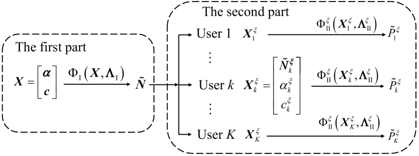
Figure 1: Illustration of the cascaded NNs.

III-C Labeled Training Samples

The optimal solutions of an MINLP problem can be found by some well-known algorithms, such as branch-and-bound (BnB) [50]. However, BnB requires a very high computational complexity, possibly approaching to the exhaustive search for some worst cases [51].

To obtain a large number of training samples, we develop an optimization algorithm that converges to the global optimal solution of problem (14) with acceptable complexity. First, we validate the feasibility of problem (14), i.e., whether the radio resources, $N^{\rm max}$ and $P^{\max}$, can guarantee the QoS requirements of all the $K$ users. If the problem is feasible, then we find the optimal solution of problem (14).

III-C1 Feasibility of Problem (14)

To find out whether problem (14) is feasible, we minimize the required total transmit power $\sum_{k\in\cal K^{\xi}}P_{k}^{\xi}$ subject to the other constraints, if the required total transmit power is less than $P^{\max}$, then the problem is feasible. Otherwise, it is infeasible. The required minimum total transmit power can be found by solving the following problem,

$$\min_{P_{k}^{\xi},N_{k}^{\xi}}\;\sum_{k\in\cal K^{\xi}}P_{k}^{\xi},$$ (18)

s.t. $$\eqref{sb1_tot},\eqref{dtCon},\eqref{dsCon},\;\text{and}\;\eqref{err},$$

To solve problem (18), we find the optimal bandwidth allocation that minimizes the total required transmit power. For a given bandwidth allocation, $N_{k}^{\xi}$, the expressions in (1), (8) and (11) are monotonous with respect to $P_{k}^{\xi}$. If we can drive the closed-form expressions of the multiple integrals in (1), (8) and (11), then the binary search can be used to obtain the minimum transmit power that is required to ensure constraints (2), (9), and (12), $P_{k}^{\xi}(N_{k}^{\xi})$. However, the closed-form expressions are not available, and this approach is time-consuming since the system needs to compute the multiple integrals in each iteration of the binary search. To avoid computing the integrals, we adopt the stochastic gradient descent (SGD) method to find the minimum transmit power subject to constraints (2), (9), and (12), respectively. As shown in [28, 52], the SGD method is efficient in solving constrained optimization problems, where some constraints do not have closed-form expressions.

Let $x(\tau)$ be a variable obtained in the $\tau$-th iteration. For delay-tolerant services, by substituting (1) into (2), the optimal transmit power with a given bandwidth allocation can be found through the following iterations,

$$P_{k}^{\rm t}(\tau+1)=\left[P_{k}^{\rm t}(\tau)+\phi(\tau)\left({\bar{a}_{k}}-\bar{R}_{k}^{{\rm{t}}}(\tau)\right)\right]^{+},$$ (19)

where $[x]^{+}=\max\{x,0\}$, $\phi(\tau)>0$ is the step size, and $\bar{R}_{k}^{{\rm{t}}}(\tau)$ is the average service rate in (1), which is estimated from a set of realizations of small-scale channel gains on the $N_{k}^{\rm t}$ subcarriers. From (19), we can see that if $\bar{R}_{k}^{{\rm{t}}}(\tau)>\bar{a}_{k}$, then $P_{k}^{\rm t}(\tau+1)>P_{k}^{\rm t}(\tau)$. Otherwise, $P_{k}^{\rm t}(\tau+1)<P_{k}^{\rm t}(\tau)$. As indicated in [53], with $\phi(\tau)\sim\mathcal{O}(1/\tau)$, the SGD method can converge to the unique optimal transmit power that satisfies $\bar{R}_{k}^{{\rm{t}}}={\bar{a}_{k}}$.

To obtain an unbiased gradient estimation with the SGD method, the expectation in the constraint should be linear [52]. For delay-sensitive services, we first transform constraint (9) into an equivalent form that is linear to the expectation, i.e., $\mathbb{E}_{g_{k,n}^{\rm s}}\left[\exp\left(-\theta_{k}^{\rm s}{T_{\rm c}}R_{k}^{\rm s}\right)\right]-\exp(-\theta_{k}^{\rm s}{T_{\rm c}}E_{k}^{B,\rm s})\leq 0$. Then, the optimal transmit power with a given bandwidth allocation can be found through the following iterations,

$$P_{k}^{\rm s}(\tau+1)=\left[P_{k}^{\rm s}(\tau)+\phi(\tau)\left(\exp(-\theta_{k}^{\rm s}{T_{\rm c}}R_{k}^{\rm s}(\tau))-\exp(-\theta_{k}^{\rm s}{T_{\rm c}}E_{k}^{B,\rm s})\right)\right]^{+},$$ (20)

where $R_{k}^{\rm s}(\tau)$ is the realization of the achievable rate in (3).

For URLLC services, the optimal transmit power with a given bandwidth allocation can be obtained from the following iterations,

$$P_{k}^{\rm u}(\tau+1)=\left[P_{k}^{\rm u}(\tau)+\phi(\tau)\left(\bar{\epsilon}_{k}^{\rm d,u}(\tau)-\epsilon^{\max,\rm u}\right)\right]^{+},$$ (21)

where $\bar{\epsilon}_{k}^{\rm d,u}(\tau)$ is the realization of the decoding error probability in (11).

TABLE II: Bandwidth Allocation Algorithm for Solving Problem (18)

0:  Large-scale channel gains $\alpha_{k}^{\xi}$ and QoS constraints $c_{k}^{\xi}$.

1:  Initialize $N_{k}^{\xi}=1,\forall k\in\cal K^{\xi}$.

2:  Compute $\Delta P_{k}^{\xi}(N_{k}^{\xi})=P_{k}^{\xi}(N_{k}^{\xi})-P_{k}^{\xi}({N}_{k}^{\xi}+1),\forall k\in\cal K^{\xi}$.

3:  while  $\sum_{k\in\cal K^{\xi}}N_{k}^{\xi}\leq N^{\rm max}$ and $\Delta P_{k^{*}}^{\xi}(N_{k^{*}}^{\xi})>0$ do

4:     $k^{*}:=\arg\max_{k\in\cal K^{\xi}}\Delta P_{k}^{\xi}(N_{k}^{\xi})$.

5:     $N_{k^{*}}^{\xi}:=N_{k^{*}}^{\xi}+1$.

6:     Update $P_{k^{*}}^{\xi}(N_{k^{*}}^{\xi})$ and $P_{k^{*}}^{\xi}({N}_{k^{*}}^{\xi}+1)$ according to (2), (9), and (12).

7:     $\Delta P_{k^{*}}^{\xi}(N_{k^{*}}^{\xi}):=P_{k^{*}}^{\xi}(N_{k^{*}}^{\xi})-P_{k^{*}}^{\xi}({N}_{k^{*}}^{\xi}+1)$.

8:  end while

9:  return  $\hat{N}_{k}^{\xi}:=N_{k}^{\xi}$ and $\hat{P}_{k}^{\xi}(\hat{N}_{k}^{\xi}):=P_{k}^{\xi}(N_{k}^{\xi})$, $k=1,...,K.$

The bandwidth allocation algorithm for solving problem (18) is shown in Table II.

Step 1: Initialize bandwidth allocation with $N_{k}^{\xi}=1,\forall k$, and compute $\Delta P_{k}^{\xi}(N_{k}^{\xi})=P_{k}^{\xi}(N_{k}^{\xi})-P_{k}^{\xi}({N}_{k}^{\xi}+1),\forall k\in\cal K^{\xi}$ with the SGD method.

Step 2: Assign one more subcarrier to the user with the highest power saving, i.e.,

$$k^{*}=\arg\max_{k\in\cal K^{\xi}}\Delta P_{k}^{\xi}(N_{k}^{\xi}).$$

Step 3: Update $N_{k^{*}}^{\xi}$ and $\Delta P_{k^{*}}^{\xi}(N_{k^{*}}^{\xi})$ with the SGD method.

Finally, we execute Step 2 and Step 3 iteratively until $\sum_{k\in\cal K^{\xi}}N_{k}^{\xi}=N^{\rm max}$.

III-C2 Algorithm for Solving Problem (14)

If problem (14) is feasible, we use the algorithm in Table III to solve this problem.

Step 1 (Lines 2-10 in Table III): We find the optimal bandwidth and transmit power allocation that minimizes $P_{\rm tot}$ without the total transmit power constraint in (14b). To achieve this goal, we replace $\Delta P_{k}^{\xi}(N_{k}^{\xi})$ in Table II with

$$\Delta P_{\mathrm{tot},k}^{\xi}(N_{k}^{\xi}) \triangleq P_{\rm tot}([N_{1}^{\xi},...,N_{k}^{\xi},...,N_{K}^{\xi}])-P_{\rm tot}([N_{1}^{\xi},...,N_{k}^{\xi}+1,...,N_{K}^{\xi}])$$

$$=\Delta P_{k}^{\xi}(N_{k}^{\xi})-P^{\rm ca}N_{\rm T}.$$ (22)

Like the algorithm in Table II, each subcarrier is allocated to the user with the highest $\Delta P_{\mathrm{tot},k}^{\xi}(N_{k}^{\xi})$. The results obtained in this step is denoted by $\check{N}_{k}^{\xi}$ and $\check{P}_{k}^{\xi}(\check{N}_{k}^{\xi})$. If the equality in constraint (14a) holds with the results in this step, i.e., $\sum_{k\in\cal K^{\xi}}\check{N}_{k}^{\xi}=N^{\rm max}$, the solutions obtained from the algorithms in Tables II and III are the same. This is because the second term in (13) is fixed, and thus minimizing $\sum_{k\in\cal K^{\xi}}P_{k}^{\xi}$ is equivalent to minimizing $P_{\rm tot}$.

Step 2 (Lines 11-21 in Table III): If $\sum_{k\in\cal K^{\xi}}\check{N}_{k}^{\xi}<N^{\rm max}$, then we check whether constraint (14b) is satisfied or not. If it is satisfied, $\check{N}_{k}^{\xi}$ and $\check{P}_{k}^{\xi}(\check{N}_{k}^{\xi})$ will be returned as the outputs of the algorithm. Otherwise, more subcarriers will be assigned to the users until the transmit power constraint is satisfied (Lines 13-21 in Table III).

TABLE III: Bandwidth Allocation Algorithm for Solving Problem (14)

0:  Large-scale channel gains $\alpha_{k}^{\xi}$ and QoS constraints $c_{k}^{\xi}$.

1:  Check whether problem (14) is feasible or not with the algorithm in Table II.

2:  Initialize $N_{k}^{\xi}:=1,\forall k\in\cal K^{\xi}$, and $P_{\rm tot}([1,...,1])$.

3:  Compute $\Delta P_{\mathrm{tot},k}^{\xi}(N_{k}^{\xi}):=P_{\rm tot}([N_{1}^{\xi},...,N_{k}^{\xi},...,N_{K}^{\xi}])-P_{\rm tot}([N_{1}^{\xi},...,N_{k}^{\xi}+1,...,N_{K}^{\xi}]),\forall k\in\cal K^{\xi}$.

4:  while  $\sum_{k\in\cal K^{\xi}}N_{k}^{\xi}\leq N^{\rm max}$ and $\Delta P_{\mathrm{tot},k^{*}}^{\xi}(N_{k^{*}}^{\xi})>0$ do

5:     $k^{*}:=\arg\max_{k\in\cal K^{\xi}}\Delta P_{\mathrm{tot},k}^{\xi}(N_{k}^{\xi})$.

6:     $N_{k^{*}}^{\xi}:=N_{k^{*}}^{\xi}+1$.

7:     Update $P_{\rm tot}([N_{1}^{\xi},...,N_{k^{*}}^{\xi},...,N_{K}^{\xi}])$ and $P_{\rm tot}([N_{1}^{\xi},...,N_{k^{*}}^{\xi}+1,...,N_{K}^{\xi}])$ according to (2), (9), (12), and (13).

8:     $\Delta P_{\mathrm{tot},k^{*}}^{\xi}(N_{k^{*}}^{\xi}):=P_{\rm tot}([N_{1}^{\xi},...,N_{k^{*}}^{\xi},...,N_{K}^{\xi}])-P_{\rm tot}([N_{1}^{\xi},...,N_{k^{*}}^{\xi}+1,...,N_{K}^{\xi}])$.

9:  end while

10:  $\check{N}_{k}^{\xi}:=N_{k}^{\xi}$ and $\check{P}_{k}^{\xi}(\check{N}_{k}^{\xi}):=P_{k}^{\xi}(N_{k}^{\xi})$, $\forall k=1,...,K$.

11:  if $\sum_{k\in\cal K^{\xi}}\check{P}_{k}^{\xi}(\check{N}_{k}^{\xi})\leq P^{\rm max}$ then

12:     return  $\dot{N}_{k}^{\xi}:=\check{N}_{k}^{\xi},\dot{P}_{k}^{\xi}(\dot{N}_{k}^{\xi}):=\check{P}_{k}^{\xi}(\check{N}_{k}^{\xi})$.

13:  else

14:     $\dot{N}_{k}^{\xi}:=\check{N}_{k}^{\xi},\dot{P}_{k}^{\xi}(\dot{N}_{k}^{\xi}):=\check{P}_{k}^{\xi}(\check{N}_{k}^{\xi})$.

15:     while $\sum_{k\in\cal K^{\xi}}\dot{P}_{k}^{\xi}(\dot{N}_{k}^{\xi})\leq P^{\rm max}$ do

16:        $k^{*}:=\arg\max_{k\in\cal K^{\xi}}\Delta\dot{P}_{k}^{\xi}(\dot{N}_{k}^{\xi})$.

17:        $\dot{N}_{k^{*}}^{\xi}:=\dot{N}_{k^{*}}^{\xi}+1$.

18:        Update $\dot{P}_{k^{*}}^{\xi}(\dot{N}_{k^{*}}^{\xi})$ and $\dot{P}_{k^{*}}^{\xi}(\dot{N}_{k^{*}}^{\xi}+1)$ according to (2), (9), and (12).

19:        $\Delta\dot{P}_{k^{*}}^{\xi}(N_{k^{*}}^{\xi}):=\dot{P}_{k^{*}}^{\xi}(\dot{N}_{k^{*}}^{\xi})-\dot{P}_{k^{*}}^{\xi}(\dot{N}_{k^{*}}^{\xi}+1)$.

20:     end while

21:     return  $\dot{N}_{k}^{\xi},\dot{P}_{k}^{\xi}(\dot{N}_{k}^{\xi})$.

22:  end if

III-C3 Optimality of Algorithm for Solving Problem (14)

In this subsection, we first discuss the optimality conditions of the algorithm in Table II, and prove that the conditions are satisfied with all the three kinds of services. Then, we prove the optimality of the algorithm in Table III.

The algorithm in Table II can find the global optimal solution for problem (18) if the following two conditions hold (See proof in Appendix A).

Condition 1.

$P_{k}^{\xi}(N_{k}^{\xi})>P_{k}^{\xi}(N_{k}^{\xi}+1)$, $\forall N_{k}^{\xi}=1,...,N^{\rm max}-1.$

Condition 1 means the required transmit power decreases with the number of subcarriers.

Condition 2.

$\Delta P_{k}^{\xi}(N_{k}^{\xi})\geq\Delta P_{k}^{\xi}(N_{k}^{\xi}+1),\forall N_{k}^{\xi}=1,...,N^{\rm max}-1.$

For notational simplicity, we denote the left-hand sides of constraints (2), (9), and (12) by $f_{k}^{\xi}(P_{k}^{\xi},N_{k}^{\xi})$, $\xi\in\{\rm{t},\rm{s},\rm{u}\}$, respectively. Since the minimum transmit power is obtained when the equalities in these constraints hold, we can prove the following proposition (see proof in Appendix B).

Proposition 1.

For a constraint $f_{k}^{\xi}(P_{k}^{\xi},N_{k}^{\xi})=c^{\xi}_{k},P_{k}^{\xi}\in\mathbb{R}^{+},N_{k}^{\xi}\in\mathbb{Z}^{+}$, if there exists a continuous relaxation of the constraint, ${\mathord{\buildrel\lower 3.0pt\hbox{$\scriptscriptstyle\smile$}\over{f}}}_{k}^{\xi}(P_{k}^{\xi},{\mathord{\buildrel\lower 3.0pt\hbox{$\scriptscriptstyle\smile$}\over{N}}}_{k}^{\xi})=c^{\xi}_{k}$, where ${\mathord{\buildrel\lower 3.0pt\hbox{$\scriptscriptstyle\smile$}\over{N}}}_{k}^{\xi}\in\mathbb{R}^{+}$ and $\mathord{\buildrel{\lower 3.0pt\hbox{$\scriptscriptstyle\smile$}}\over{f}}_{k}^{\xi}(P_{k}^{\xi},\mathord{\buildrel{\lower 3.0pt\hbox{$\scriptscriptstyle\smile$}}\over{N}}_{k}^{\xi})$ is jointly concave (or convex) in $P_{k}^{\xi}$, ${\mathord{\buildrel\lower 3.0pt\hbox{$\scriptscriptstyle\smile$}\over{N}}}_{k}^{\xi}$ and increases (or decreases) with $P_{k}^{\xi}$ and ${\mathord{\buildrel\lower 3.0pt\hbox{$\scriptscriptstyle\smile$}\over{N}}}_{k}^{\xi}$, then Conditions 1 and 2 hold for the original constraint, $f_{k}^{\xi}(P_{k}^{\xi},N_{k}^{\xi})=c^{\xi}_{k},P_{k}^{\xi}\in\mathbb{R}^{+},N_{k}^{\xi}\in\mathbb{Z}^{+}$.

Delay-Tolerant Services: As proved in [20], (1) is strictly concave in $P_{k}^{\rm t}$. If $f(x)$ is concave, then $yf(x/y)$ is jointly concave in $x$ and $y$ [12]. Thus, (1) is jointly concave in $P_{k}^{\rm t}$ and $N_{k}^{\rm t}$. In addition, the Shannon’s capacity increases with transmit power and the number of subcarriers. Therefore, Condition 1 and 2 hold for delay-tolerant services.

Delay-Sensitive Services: According to the results in [21], we know that effective capacity is jointly concave in $P_{k}^{\rm s}$ and $N_{k}^{\rm s}$ and increases with $P_{k}^{\rm s}$ and $N_{k}^{\rm s}$. Therefore, Conditions 1 and 2 also hold for delay-tolerant services.

URLLC Services: Unlike the above two types of services, constraint (12) for URLLC is not convex in $P_{k}^{\rm u}$ and $N_{k}^{\rm u}$ in general. To study whether the proposed algorithm can find the optimal solution, we first consider an asymptotic scenario: $N_{\rm T}$ is large. When $N_{\rm T}$ is sufficiently large, due to channel hardening, we have [54]

$${\ln\left({1+\frac{{\alpha_{k}^{\rm{u}}g_{k,n}^{\rm{u}}P_{k}^{\rm{u}}}}{{{N_{0}}{N_{\rm{T}}}N_{k}^{\rm{u}}W}}}\right)}\to{\ln\left({1+\frac{{\alpha_{k}^{\rm{u}}P_{k}^{\rm{u}}}}{{{N_{0}}N_{k}^{\rm{u}}W}}}\right)}.$$ (23)

Then, the minimum transmit power that can satisfy constraint (12) can be derived as follows,

$$P_{k}^{\rm{u}}(N_{k}^{\rm{u}})=\frac{{{N_{0}}N_{k}^{\rm{u}}W}}{{\alpha_{k}^{\rm{u}}}}\left\{{\exp\left[{\frac{{B_{k}^{\rm{u}}\ln 2}}{{{T_{\rm{s}}}N_{k}^{\rm{u}}W}}+\frac{{f_{Q}^{-1}\left({{{\bar{\varepsilon}}^{\max{\rm{,u}}}}}\right)}}{{\sqrt{{T_{\rm{s}}}N_{k}^{\rm{u}}W}}}}\right]-1}\right\}.$$ (24)

According to the analysis in [8], $P_{k}^{\rm{u}}(N_{k}^{\rm{u}})$ first decreases with $N_{k}^{\rm{u}}$ and then increases with $P_{k}^{\rm{u}}(N_{k}^{\rm{u}})$. We denote $\acute{N}_{k}^{\rm{u}}$ as the optimal number of subcarriers that minimizes $P_{k}^{\rm{u}}(N_{k}^{\rm{u}})$. Since $\Delta P_{k}^{\rm{u}}(\acute{N}_{k}^{\rm{u}})<0$, the number of subcarriers assigned to the $k$-th URLLC user will not exceed $\acute{N}_{k}^{\rm{u}}$. Moreover, $P_{k}^{\rm{u}}(N_{k}^{\rm{u}})$ is convex and decreases with $N_{k}^{\rm{u}}$ in the region $[1,\acute{N}_{k}^{\rm{u}}]$ [8]. Therefore, Conditions 1 and 2 hold for URLLC services in the asymptotic scenario.

For non-asymptotic scenarios, the expectation in (11) is a $N_{k}^{u}$-fold integral. Since the number of folds increases with the optimization variable, $N_{k}^{u}$, one can neither derive a closed-form expression nor get any strict proof. When the number of antennas is large, e.g., $N_{\rm T}>32$, (24) is a good approximation of the required transmit power in the non-asymptotic scenarios, and hence Conditions 1 and 2 hold. For systems with small numbers of antennas, we will validate Conditions 1 and 2 via numerical results with typical parameters in 5G cellular networks.

The above analysis indicates that the algorithm in Table II can find the optimal solution of problem (18). In addition, by solving problem (18), we know whether problem (14) is feasible or not. If the problem is feasible, the following proposition shows that the algorithm in Table III can find the optimal solution to the problem.

Proposition 2.

The algorithm in Table III can find the global optimal solution for problem (14) if Conditions 1 and 2 hold.

Proof.

See proof in Appendix C. ∎

III-D Train the Cascaded NNs

With the algorithm in Table III, we can obtain a labeled training sample, $\boldsymbol{N}^{*}$ and $\boldsymbol{P}^{*}$, for any given input $\boldsymbol{X}$. To obtain enough labeled training samples, we randomly generate a large number of inputs and find the corresponding optimal solutions. One part of the data is used to train the NNs, and the other part of the data is used to test the performance of the NNs.

The parameters of the NNs are initialized with Gaussian distributed random variables with zero mean and unit variance. In each training epoch, a batch of training samples is randomly selected from all the training samples to train the NNs. The parameters of $\Phi_{\rm I}$ are optimized with the Adam algorithm [55] to minimize a loss function, defined as $\mathcal{L}_{\rm I}(\varLambda_{\rm I})=\frac{1}{M_{t}}\sum_{m_{t}=1}^{M_{t}}(\log(\boldsymbol{N}^{*}_{m_{t}}+1)-\log(\tilde{\boldsymbol{N}}_{m_{t}}+1))^{2}$, where ${M_{t}}$ is the number of training samples in each batch. Similarly, we optimize the parameters of $\Phi^{\xi}_{\rm I}$ to minimize $\mathcal{L}_{\rm II}(\varLambda_{\rm II}^{\xi})=\frac{1}{M_{t}}\sum_{m_{t}=1}^{M_{t}}(\log(\boldsymbol{P}^{*}_{m_{t}}+1)-\log(\tilde{\boldsymbol{P}}_{m_{t}}+1))^{2}$. When the value of a loss function is below a required threshold, the difference between the outputs of the NNs and the optimal resource allocation is small enough, and the outputs of the NNs are near-optimal.

III-E Complexity of Deep Learning Algorithms

Since the cascaded NNs are made up of multiple FNNs, we first analyze the complexity of the FNN and then extend the results to the cascaded NNs.

III-E1 Fast Resource Allocation

After the training phase, the forward propagation algorithm is applied to compute the output of a neural network for fast resource allocation. The processing time of the forward propagation algorithm is determined by the numbers of three kinds of operations to be executed, i.e., “$+$”, “$\times$”, and “$\max(0,\cdot)$” in the ReLU function. We first derive the number of multiplications that is required to compute the output of the FNN, which is denoted by $N_{\rm FNN}^{\rm FP}$. According to (15), the numbers of multiplications for computing the output of the $l$-th layer are $n_{\rm FNN}^{[l]}\times n_{\rm FNN}^{[l+1]}$, where $n_{\rm FNN}^{[l]}$ is the number of neurons in the $l$-th layer. Thus, we have

$$N_{\rm FNN}^{\rm FP}=\sum_{l=0}^{L_{\rm FNN}-1}n_{\rm FNN}^{[l]}\times n_{\rm FNN}^{[l+1]}.$$ (25)

Since the cascaded NNs consist of multiple FNNs, from (25), we can obtain the numbers of multiplications required to compute the output of the cascaded NNs,

$$N_{\rm CAS}^{\rm FP}=\sum_{l=0}^{L_{\rm I}-1}n_{\rm I}^{[l]}\times n_{\rm I}^{[l+1]}+M_{T}\sum_{l=0}^{L_{\rm II}-1}n_{\rm II}^{[l]}\times n_{\rm II}^{[l+1]},$$ (26)

where $L_{\rm I}$ and $L_{\rm II}$ are the number of layers of $\Phi_{\rm I}$ and $\Phi_{\rm II}$, respectively, $n_{\rm I}^{[l]}$ and $n_{\rm II}^{[l]}$ are the number of neurons in the $l$-th layer of $\Phi_{\rm I}$ and $\Phi_{\rm II}$, respectively, and $M_{T}$ is the types of services. It is not hard to see that the number of additive operations is also $N_{\rm CAS}^{\rm FP}$ and the number of ReLU operations is much smaller than $N_{\rm CAS}^{\rm FP}$. Thus, the complexity of the forward propagation algorithm with the cascaded NNs is $\mathcal{O}(N_{\rm CAS}^{\rm FP})$, which is low enough to be implemented in real-world networks for optimizing resource allocation in real time [56].

III-E2 Training Algorithm

In the training phase, the Adam algorithm is used to optimize the parameters of FNNs, where the backward propagation algorithm is used to compute the gradients of the loss function with respect to the parameters in each layer [55]. Similar to the forward propagation algorithm that computes the output from the first layer to the last layer, the backward propagation algorithm computes the gradient of the loss function with respect to the parameters from the last layer to the first layer. The complexity of the backward propagation algorithm is the same as the forward propagation algorithm, $\mathcal{O}(N_{\rm CAS}^{\rm FP})$. If there are $N_{\rm ep}$ epochs in the training phase and $M_{t}$ training samples are selected to train the NNs in each epoch, then the computing complexity for training the FNN and the cascaded NNs is $\mathcal{O}(N_{\rm ep}M_{t}N_{\rm FNN}^{\rm FP})$ and $\mathcal{O}(N_{\rm ep}M_{t}N_{\rm CAS}^{\rm FP})$, respectively.

III-E3 Finding Labeled Training Samples

Before training the NNs, the optimization algorithm in Table III is applied to find the labeled training samples. In each iteration, the algorithm assigns one more subcarrier to one of the users. Thus, the number of iterations does not exceed $N^{\max}$. Within each iteration, the algorithm needs to compute the value of $\Delta P_{\mathrm{tot},k}^{\xi}(N_{k}^{\xi})$ by using the SGD method in (19), (20) and (21). Denote the computing complexity of the SGD method by $\Omega_{P}$. Then, the complexity of the algorithm in Table III is ${\mathcal{O}}(M_{t}^{\rm tot}N^{\max}\Omega_{P})$, where $M_{t}^{\rm tot}$ is the total number of labeled training samples. The SGD method is an iterative algorithm and the convergence speed depends on how fast the learning rate decreases and the required accuracy of the final results. As suggested by [53], the learning rate cannot decrease too fast to ensure convergence. In general, it takes thousands of steps to converge to an accurate result, i.e., the transmit power required to guarantee the QoS constraints. Therefore, the optimization algorithm in Table III can hardly find the optimal resource allocation every few seconds according to the variations of the large-scale channel gains and the features of packet arrival processes.

IV Deep Transfer Learning in Non-Stationary Wireless Networks

Since the cascaded NNs are trained offline, it only works well in stationary wireless networks. However, real-world wireless networks are highly dynamic and non-stationary. There are a lot of hidden variables that are not included in the input of the cascaded NNs but have significant impacts on the optimal solution. For example, the optimal resource allocation for delay-sensitive and URLLC services depends on distributions of small-scale channel gains as well as the types of services in the network. If these distributions and parameters change, a NN trained offline is no longer a good approximation of the optimal resource allocation policy in the new scenario [19]. Such an issue is known as the task mismatch problem [57].

A straightforward approach is to train a new NN from scratch in a new scenario. When the hidden variables change, the system can hardly obtain a large number of training samples in the new scenario. This is because the algorithm in Table III cannot be executed in real time. To update the NN with a few training samples, we apply deep transfer learning.

IV-A Preliminary of Deep Transfer Learning

The learning process is to accomplish a learning task based on a data domain. According to the definitions in [57], a domain consists of a feature space and the corresponding marginal probability distribution, e.g., $\boldsymbol{X}$ and its distribution. A task consists of a label space and an objective predictive function that maps from $\boldsymbol{X}$ to $\boldsymbol{Y}^{*}$. The function is not observed but learned from the training samples, i.e., $\{\boldsymbol{X},\boldsymbol{Y}^{*}\}$. The basic idea of transfer learning is to exploit the knowledge from a well-trained source task to a new target task [58].

Fine-tuning is the most widely used method in deep transfer learning [59]. The basic idea is to fix the parameters in the first a few layers and update the parameters in the last a few layers. In deep transfer learning, parts of the well-trained NN of the source task are reused in the NN of the target task. In this way, the number of labeled training samples are needed to fine-tune the new NN is much less than that needed to train a new NN with randomly initialized parameters (i.e., learning from scratch).

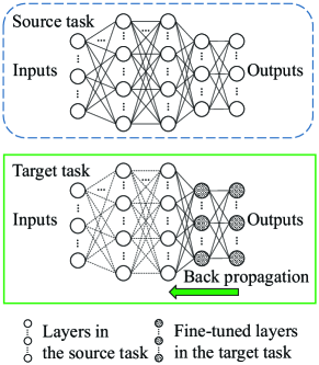
(a) Non-stationary wireless channels.

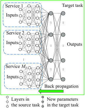
(b) Multiple types of services.

Figure 2: Deep transfer learning.

IV-B Transfer Learning with Non-Stationary Wireless Channels

In wireless communications, the distribution of small-scale channel gains may change over time. For example, the BS may switch ON/OFF some antennas. When the number of active antennas changes, the distribution of $g_{k}$ becomes different. For the cascaded NNs proposed in the previous section, the system fine-tunes the last a few layers of $\Phi_{\rm I}$ as illustrated in Fig. 2(a). Since the power allocation policy depends on the distribution of wireless channels, the system fine-tunes all the layers of $\Phi_{\rm II}^{\xi}$.

IV-C Transfer Learning with Different Types of Services

In a wireless network, the service requests are highly dynamic. In other words, the number of different types of services in the wireless networks varies significantly over time. Thus, the system needs to update the NN according to the QoS requirements of different types of services. In the simulation, only one labeled training sample can be obtained in each epoch. Thus, the number of training samples used in transfer learning equals to the number of epochs it takes to converge.

IV-C1 Transfer Learning from Delay-tolerant Services to Another Type of Services

For both delay-sensitive and URLLC services, the delay and reliability requirements depend on specific applications. Training NNs for all kinds of applications is not possible in practice. To overcome this difficulty, we first train a NN to approximate the optimal resource allocation policy of delay-tolerant services. Then, we fine-tune the NN for delay-sensitive and URLLC services. With the cascaded NNs in the previous section, the system needs to fine-tune the last a few layers of $\Phi_{\rm I}$ with the method in Fig. 2(a). Since the power allocation policy depends on the QoS requirement of each service, all the layers of $\Phi^{\xi}_{\rm II}$ should be updated.

IV-C2 Transfer Learning from a Single Type of Services to Multiple Types of Services

If there are $M_{T}$ types of services in the network, then there are $2^{M_{T}}$ possible combinations with different types of services. In 5G networks, $M_{T}$ will be large, and it is impossible to train a NN for each combination. If we have a well-trained NN for each type of services (i.e., source task), then by replacing the last a few layers of each NN, we can construct a new NN as that in Fig. 2(b). With the cascaded NNs, we only need to update $\Phi_{\rm I}$ for bandwidth allocation. The power allocation for each user is determined by $\Phi^{\xi}_{\rm II}$, which is the same as that in the source task. The algorithm is summarized in Table IV.

TABLE IV: Deep Transfer Learning for Multiple Types of Services

0:  Large-scale channel gains $\alpha_{k}^{\xi}$ and QoS constraints $c_{k}^{\xi}$.

1:  Train a NN for delay-tolerant services.

2:  Initialize an empty set $\mathcal{S}_{T}$

3:  for the $m$-th type of services, $m\in\{1,...,M_{T}\}$ do

4:     if the $m$-th type of services is requested by some users then

5:        $\mathcal{S}_{T}:=\mathcal{S}_{T}\cup\{m\}$

6:        Collect a few training samples for the $m$-th type of services with the algorithm in Table III.

7:        Initialize parameters of a new NN with the parameters in the well-trained NN.

8:        Fine-tuning the last a few layers of the new NN with the method in Section IV-C1.

9:     end if

10:     Stack the NNs for all $m\in\mathcal{S}_{T}$ according to Fig. 2(b).

11:  end for

12:  Collect a few training samples for multiple types of services with the algorithm in Table III.

13:  Fine-tune the stacked NNs with the method in Section IV-C2.

14:  return  the parameters of the fine-tuned NNs.

V Simulation and Numerical Results

In the considered scenario, the coverage of the BS is $200$ meters. Users are uniformly distributed around the BS. The path loss model is $35.3+37.6\log_{10}(d)$, where $d$ is the distance (meters) between the BS and a user. The shadowing is lognormal distributed with $8$ dB standard deviation. The small-scale channels are Rayleigh fading and the distribution of the small-scale channel gains follows $f_{g}(x)=\frac{1}{(N_{\rm T}-1)!}x^{N_{\rm T}-1}e^{-x}$. The rest of the simulation parameters are summarized in Table V, unless specified otherwise.

TABLE V: Parameters in Simulation

Maximal transmit power of the BS $P^{\max}$	$46$ dBm
Duration of one TTI $T_{\rm s}$	$0.125$ ms [60]
Bandwidth of each subcarrier $W$	$120$ kHz [60]
Channel coherence time $T_{\rm c}$	$5$ ms [60]
Single-sided noise spectral density $N_{0}$	$-174$ dBm/Hz
Number of bytes in a packet $B_{k}^{\rm u}$	$[20,64]$ bytes [2]
Average data arrival rate of delay-tolerant users $\bar{a}_{k}$	$[50,100]$ KB/s
Packet loss probability of URLLC $\epsilon^{\rm max,u}$	$5\times 10^{-8}$
Circuit power consumption per antenna $N^{\max}P^{\rm ca}$	$50$ mW [48]
Fixed circuit power $P_{0}^{\rm c}$	$50$ mW [48]
Power amplifier efficiency $\rho$	$0.5$ [48]
Average packet arrival rate of delay-sensitive services $\nu^{\rm a}$	$[100,1000]$ packets/s
Average packet size of delay-sensitive services $1/\nu^{\rm s}$	$[1,20]~{}\text{kbits}$
Delay bound of delay-sensitive user $D_{k}^{\rm q,s}$	$50$ ms
Maximal tolerable delay bound violation probability of delay-sensitive user $\epsilon_{k}^{\rm q,s}$	$10^{-2}$

V-A Validating the Properties of URLLC

In this subsection, we first validate that Conditions 1 and 2 hold in non-asymptotic scenarios of URLLC. In Fig 3, we randomly select a user and illustrate the monotonicity of $P_{k}^{\rm u}(N_{k}^{\rm u})$ and $\Delta P_{k}^{\rm u}(N_{k}^{\rm u})$. The results show that even when the number of antennas is not large, such as $N_{\rm T}=4,8,16$, Conditions 1 and 2 hold. The results indicate that the algorithms in Tables II and III can converge to the optimal solutions.

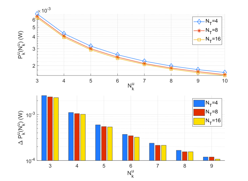
Figure 3: Validating Conditions 1 and 2 for URLLC services.

V-B Performance Evaluation

In this subsection, we evaluate the performance achieved by the deep learning method in Sections III and III-B. In the scenarios with multiple types of services, the ratio of the number of users requesting the three types of services is set to be $1:1:1$. The algorithm in Table III is used to find the optimal solutions of problem (14) with $10000$ inputs, where $N^{\max}=256$, $N_{T}=64$ and $K^{\xi}=20$. The first $9000$ samples are used to train the NNs and the last $1000$ samples are used to test the performance of them. In each epoch, $M_{t}=128$ training samples are randomly selected from $9000$ training samples, and the learning rate is set to be $0.001$. The DL algorithm is implemented in Python with TensorFlow 1.11.

Each neural network consists of one input layer, one output layer, and ${L}_{\text{hidden}}^{\xi}$ hidden layers, where each hidden layer has $N_{\text{neurons}}^{\xi}$ neurons. The input and output layers of the FNN are defined after (16). The input and output layers of the cascaded NNs are defined in Fig. 1. The hyper-parameters (i.e., ${L}_{\text{hidden}}^{\xi}$ and $N_{\text{neurons}}^{\xi}$) for different types of services can be found in Table VI. We selected the hyper-parameters by trial and error, where ${L}_{\text{hidden}}^{\xi}$ ranges from $1$ to $10$ and $N_{\text{neurons}}^{\xi}$ ranges from $200$ to $1000$. The hyper-parameters in Table VI can achieve the best performance according to our experience.

TABLE VI: Hyper-parameters of NNs

Service type	FNN		Cascaded NNs
			The $1$st part $\Phi_{\rm I}$		The $2$nd part $\Phi^{\xi}_{\rm II}$
	${L}_{\text{hidden}}^{\xi}$	$N_{\text{neurons}}^{\xi}$	${L}_{\text{hidden}}^{\xi}$	$N_{\text{neurons}}^{\xi}$	${L}_{\text{hidden}}^{\xi}$	$N_{\text{neurons}}^{\xi}$
Delay-tolerant	4	800	4	800	4	20
Delay-sensitive	5	600	5	600	4	20
URLLC	4	600	4	600	4	20

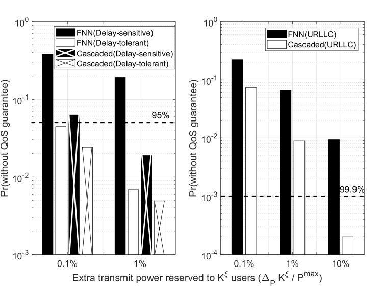
Figure 4: Probability without QoS guarantee v.s. extra transmit power reserved to the users.

In Fig. 4, we show the QoS achieved by the FNN and the cascaded NNs. Specifically, the relation between the probability without QoS guarantee (i.e., the probability that the transmit power allocated to a user is smaller than the minimum transmit power that is required to satisfy the QoS constraint of the user, $\Pr\{\Phi_{\rm II}^{\xi}(\boldsymbol{X}_{k}^{\xi},\varLambda_{\rm II}^{\xi})+\Delta_{P}<P_{k}^{\xi}(\tilde{N}_{k}^{\xi})\}$). and the extra transmit power reserved to all the $K^{\xi}$ users, $\Delta_{P}K^{\xi}$, is provided. For each type of service, we set $|\mathcal{K}^{\xi}|=20$. The results are evaluated with $1000$ testing samples.

From Fig. 4, we can observe that the cascaded NNs can achieve better QoS compared with the FNN. For example, by reserving $10$% of $P^{\max}$ extra transmit power to the $20$ URLLC users, the cascaded NNs can satisfy the QoS requirement with a probability of $99.98\%$. However, the FNN can only satisfy the QoS requirement with a probability of $99.2$%. For other types of services, the cascaded NNs also outperform the FNN in terms of achieving better QoS. This validates that the cascaded NNs can improve the QoS for all types of services.

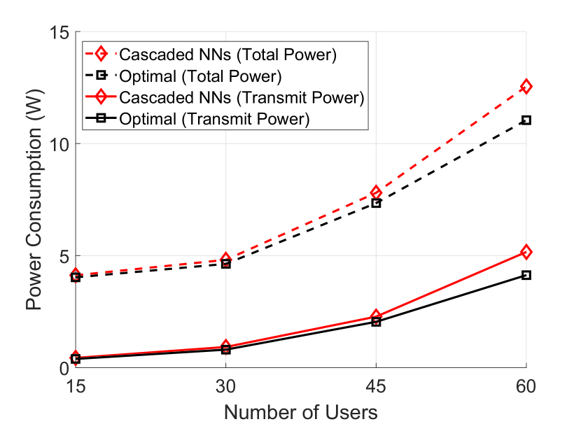
Figure 5: Power consumption v.s. number of users when $N_{T}=64$ and $N^{\max}=256$.

The total power consumption and transmit power achieved with different schemes are illustrated in Fig. 5. We compare the performance of the cascaded NNs with the optimal solutions obtained with the algorithm in Tables II and III (with legend ‘Optimal’). For the deep learning method, we train the cascaded NNs when $K^{\rm t}=K^{\rm s}=K^{\rm u}=20$, which is close to the maximal number of users that can be served with the given radio resources. In practical systems, the number of users is dynamic. When the number of users is less than $60$, we do not change the dimension of the input, but set $c_{k}^{\xi}=0$. It means that the required data rates, effective bandwidth or packet sizes of some users are zero. In this case, no resource will be assigned to them. The performance with the cascaded NNs is close to the optimal solutions. This implies the cascaded NNs are a good approximation of the optimal policy.

V-C Performance with Transfer Learning

Since NNs are used to approximate the optimal resource allocation policy, the accuracy is defined as follows,

$$\eta=1-\text{Error}=1-\frac{{P}_{\rm tot}(\tilde{\boldsymbol{N}},\tilde{\boldsymbol{P}})-P_{\rm tot}(\boldsymbol{N}^{*},\boldsymbol{P}^{*})}{P_{\rm tot}(\boldsymbol{N}^{*},\boldsymbol{P}^{*})},$$ (27)

which reflects the gap between the outputs of NNs and the optimal solutions.

To show that convergence time of different methods, we provide the relation between the numbers of training epochs and the accuracy. The transfer learning methods that fine-tune the well-trained NNs in the source domain and task are compared with the benchmark that trains new NNs with randomly initialized parameters (with legend ‘Random initialization’ and initializing each parameter with a zero mean and unit variance Gaussian variable). In this subsection, we only consider the cascaded NNs since this structure can guarantee the QoS constraints with a high probability.

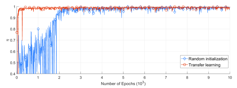
Figure 6: Accuracy v.s. the number of training epochs when $N_{T}$ varies, where $N^{\max}=256$, $K^{\rm u}=20$.

V-C1 Transfer learning with non-stationary wireless channels

The training samples in the source domain and task are obtained when $N_{\rm T}=16$. The training samples in the target domain and task are obtained when $N_{\rm T}=64$. With different numbers of antennas, the distribution of small-scale channel gains varies. With transfer learning, the first $3$ layers of $\Phi_{\rm I}$ are fixed. The last layer of $\Phi_{\rm I}$ and $\Phi^{\xi}_{\rm II}$ are fine-tuned. The results in Fig. 6 show that with transfer learning, only $400$ epochs ($400$ training samples in the new scenario) are needed to achieve around $0.98$ accuracy, while $2000$ epochs ($2000$ training samples in the new scenario) are needed to achieve the same accuracy with random initialization.

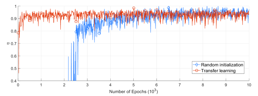
Figure 7: Accuracy v.s. the number of training epochs, where the target task is resource allocation for delay-sensitive services, $N^{\max}=256$, $N_{T}=64$ and $K^{\xi}=20$.

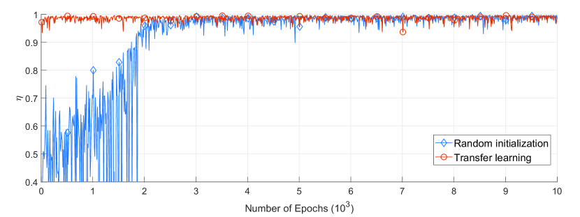
Figure 8: Accuracy v.s. the number of training epochs, where the target task is resource allocation for URLLC, $N^{\max}=256$, $N_{T}=64$ and $K^{\xi}=20$.

V-C2 Transfer learning from delay-tolerant services to another type of services

We first train cascaded NNs for delay-tolerant services with $9000$ labeled training samples. Then, we fine-tune the well-trained cascaded NNs with new labeled training samples of another type of services. Specifically, the first $3$ layers of $\Phi_{\rm I}$ are fixed and the NNs in the second part, $\Phi_{\rm II}^{\rm t}$, are replaced with NNs for delay-sensitive services, $\Phi_{\rm II}^{\rm s}$.

The results in Fig. 7 show that the transfer learning method can achieve $0.9$ accuracy with around $150$ epochs ($150$ training samples in the new scenario), while it takes $2500$ epochs for the random initialization method to achieve the same accuracy ($2500$ training samples in the new scenario). A similar conclusion can be observed from the results in Fig. 8. By comparing the results in Figs. 7 and 8, we can see that the accuracy of transfer learning for URLLC is higher than that for delay-sensitive services. As shown in Table VI, to achieve good performance for delay-sensitive services, we need $5$ hidden-layers in $\Phi_{\rm I}$. However, for delay-tolerant and URLLC services, only $4$ hidden-layers are needed in $\Phi_{\rm I}$. Since we use the same hyper-parameter in the source task and target tasks, deep transfer learning achieves higher accuracy for URLLC compared with delay-sensitive services.

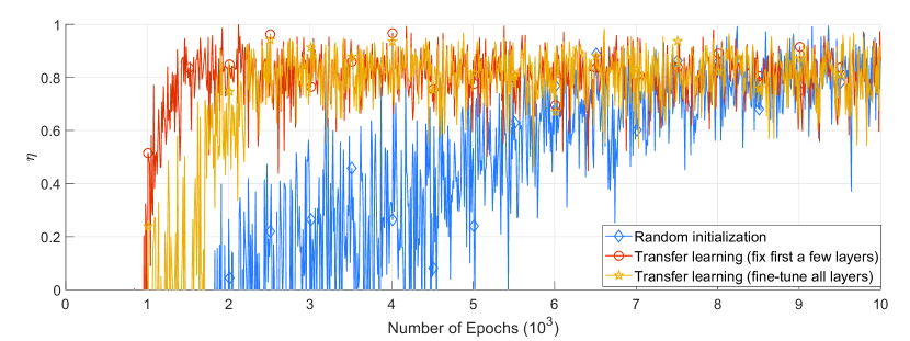
Figure 9: Transfer knowledge from networks with a single type of services to networks with multiple types of services, $N^{\max}=256$, $N_{T}=64$ and $K^{\xi}=20$.

V-C3 Transfer knowledge from a single type of services to multiple types of services

To apply transfer learning in bandwidth allocation, the structure in Fig. 2(b) is adopted. Specifically, the output layers of the three NNs for the three types of services are replaced with an output layer with $(K^{\rm t}+K^{\rm s}+K^{\rm u})$ neurons. With deep transfer learning, we can either fix the first a few-layers or fine-tune all the layers, i.e., the curves with legends ‘Transfer learning (fix first a few layers)’ and ‘Transfer learning (fine-tune all layers)’, respectively. For the neural network with legend ‘Transfer learning (fix first a few layers)’, we fixed the first a few layers and fine-tuned the last $2$ layers. The performance of them is compared with a benchmark that trains a NN with randomly initialized parameters (with legend ‘Random initialization’), where the NN includes $4$ hidden layers, and each of them has $800$ neurons. The results in Fig. 9 show that ‘Transfer learning (fix first a few layers)’ outperforms ‘Transfer learning (fine-tune all layers)’ in the first $2500$ epochs (with less than $2500$ training samples), and they achieve the same performance after the $2500$ epoch (with more than $2500$ training samples). This indicates that there is no need to fine-tune all the layers of the NN. Compared with the benchmark, transfer learning can achieve higher accuracy in the first $8000$ training epochs. By the end of the training phase, the performance of them is almost the same.

VI Conclusion

In this work, we studied how to use deep learning in resource allocation with diverse QoS requirements in 5G networks. Specifically, we proposed an optimization algorithm that can converge to the optimal solution of an optimization problem that minimizes the total power consumption for delay-tolerant, delay-sensitive, and URLLC services. The obtained optimal solutions were used as labeled training samples to train NNs that approximate the optimal policy. To guarantee the diverse QoS requirements in non-stationary wireless networks, we designed cascaded NNs and fine-tuned their parameters with deep transfer learning. Our simulation results validated that the proposed deep transfer learning framework converges quickly when the wireless channels or the service requests are non-stationary.

Appendix A Proof of Optimality of the Algorithm in Table II

Proof.

We denote the objective function in (18) as $f(\boldsymbol{N})=\sum_{k\in\cal K^{\xi}}P_{k}^{\xi}(N_{k}^{\xi})$ in this Appendix, where $\boldsymbol{N}=[N_{1}^{\xi},...,N_{K}^{\xi}]^{\rm T}$. The outcome of the algorithm in Table II is denoted by $\boldsymbol{N}^{*}=[N_{1}^{\xi*},...,N_{K}^{\xi*}]^{\rm T}$. To prove the optimality of the proposed algorithm, we only need to prove that for any bandwidth allocation scheme $\boldsymbol{N}^{\prime}=[N_{1}^{\xi^{\prime}},...,N_{K}^{\xi^{\prime}}]^{\rm T}$, $f(\boldsymbol{N}^{*})\leq f(\boldsymbol{N}^{\prime})$ holds.

The difference between $\boldsymbol{N}^{*}$ and $\boldsymbol{N}^{\prime}$ is denoted by

$$\Delta\boldsymbol{N}=\boldsymbol{N}^{\prime}-\boldsymbol{N}^{*}=[\Delta N_{1},\Delta N_{2},...,\Delta N_{K}]^{\rm T}.$$ (A.1)

We further denote that

$$\boldsymbol{N}^{+}=[\max(0,\Delta N_{1}),...,\max(0,\Delta N_{K})],$$

$$\boldsymbol{N}^{-}=[-\min(0,\Delta N_{1}),...,-\min(0,\Delta N_{K})].$$

Then, we can obtain a bandwidth allocation policy $\boldsymbol{N}^{0}=\boldsymbol{N}^{*}-\boldsymbol{N}^{-}=\boldsymbol{N}^{\prime}-\boldsymbol{N}^{+}$.

The required transmit power with policy $\boldsymbol{N}^{0}=[N^{0}_{1},...,N^{0}_{K}]$ is $f(\boldsymbol{N}^{0})$. Based on $\boldsymbol{N}^{0}$, if we allocate $(N^{\max}-\sum_{k=1}^{K}N_{k}^{0})$ extra subcarriers to the users according to $\boldsymbol{N}^{+}$, the amount of power saving is $f(\boldsymbol{N}^{0})-f(\boldsymbol{N}^{\prime})$. If we allocate $(N^{\max}-\sum_{k=1}^{K}N_{k}^{0})$ subcarriers according to $\boldsymbol{N}^{-}$, then the amount of power saving is $f(\boldsymbol{N}^{0})-f(\boldsymbol{N}^{*})$.

The amount of power saving with the above two approaches can be expressed as the sum of $(N^{\max}-\sum_{k=1}^{K}N_{k}^{0})$ terms, i.e.,

$$f(\boldsymbol{N}^{0})-f(\boldsymbol{N}^{\prime})=\sum_{k^{+}\in\cal K^{+}}\sum_{n=N_{k^{+}}^{0}}^{N_{k^{+}}^{{}^{\prime}}-1}\Delta P_{k^{+}}(n),$$ (A.2)

$$f(\boldsymbol{N}^{0})-f(\boldsymbol{N}^{*})=\sum_{k^{-}\in\cal K^{-}}\sum_{n=N_{k^{-}}^{0}}^{N_{k^{-}}^{*}-1}\Delta P_{k^{-}}(n),$$ (A.3)

where $\mathcal{K}^{+}=\{k|\Delta N_{k}>0\}$ and $\mathcal{K}^{-}=\{k|\Delta N_{k}<0\}$.

According to Condition 1 and 2, we have

$$\Delta P_{k^{+}}(N_{k^{+}}^{0}) \geq\Delta P_{k^{+}}(N_{k^{+}}^{0}+1)\geq...\geq\Delta P_{k^{+}}(N_{k^{+}}^{{}^{\prime}}-1),\forall k^{+}\in\mathcal{K}^{+}.$$ (A.4)

$$\Delta P_{k^{-}}(N_{k^{-}}^{0}) \geq\Delta P_{k^{-}}(N_{k^{-}}^{0}+1)\geq...\geq\Delta P_{k^{-}}(N_{k^{-}}^{*}-1),\forall k^{-}\in\mathcal{K}^{-}.$$ (A.5)

With the proposed algorithm, a subcarrier will be assigned to the user with the highest power saving. Thus, we have

$$\Delta P_{k^{-}}(N_{k^{-}}^{*}-1)\geq\Delta P_{k^{+}}(N_{k^{+}}^{0}),\forall k^{+}\in\mathcal{K}^{+},\forall k^{-}\in\mathcal{K}^{-}.$$ (A.6)

Since $\Delta P_{k^{-}}(N_{k^{-}}^{*}-1)$ is the last term in (A.5) and $P_{k^{+}}(N_{k^{+}}^{0})$ is the first term in (A.4), we can obtain that each term in the right-hand side of (A.2) is smaller than any term in the right-hand side of (A.3). Therefore, we have $f(\boldsymbol{N}^{0})-f(\boldsymbol{N}^{\prime})\leq f(\boldsymbol{N}^{0})-f(\boldsymbol{N}^{*})$, and hence $f(\boldsymbol{N}^{*})\leq f(\boldsymbol{N}^{\prime})$. This completes the proof. ∎

Appendix B Proof of Property 1

Proof.

For notational simplicity, we replace $\mathord{\buildrel{\lower 3.0pt\hbox{$\scriptscriptstyle\smile$}}\over{f}}_{k}^{\xi}(P_{k}^{\xi},\mathord{\buildrel{\lower 3.0pt\hbox{$\scriptscriptstyle\smile$}}\over{N}}_{k}^{\xi})$ with $f_{k}^{\xi}(P_{k}^{\xi},N_{k}^{\xi})$ in this appendix. We first derive the first-order derivatives of the right-hand and the left-hand sides of $f_{k}^{\xi}(P_{k}^{\xi},N_{k}^{\xi})=c^{\xi}_{k}$, i.e.,

$$\frac{\partial f_{k}^{\xi}(P_{k}^{\xi},N_{k}^{\xi})}{\partial N_{k}^{\xi}}+\frac{\partial f_{k}^{\xi}(P_{k}^{\xi},N_{k}^{\xi})}{\partial P_{k}^{\xi}}\frac{\partial P_{k}^{\xi}}{\partial N_{k}^{\xi}}=0.$$ (B.1)

Since $f_{k}^{\xi}(P_{k}^{\xi},N_{k}^{\xi})$ increases with both $N_{k}^{\xi}$ and $P_{k}^{\xi}$, we have $\frac{\partial f_{k}^{\xi}(P_{k}^{\xi},N_{k}^{\xi})}{\partial N_{k}^{\xi}}>0$ and $\frac{\partial f_{k}^{\xi}(P_{k}^{\xi},N_{k}^{\xi})}{\partial P_{k}^{\xi}}>0$. According to (B.1), we can see that $\frac{\partial P_{k}^{\xi}}{\partial N_{k}^{\xi}}<0$, i.e., $P_{k}^{\xi}$ decreases with $N_{k}^{\xi}$. Therefore, Condition 1 holds.

From (B.1), we further derive the second-order derivative, i.e.,

$$\underbrace{\frac{\partial^{2}f_{k}^{\xi}(P_{k}^{\xi},N_{k}^{\xi})}{\partial(P_{k}^{\xi})^{2}}}_{a}\underbrace{\left(\frac{\partial P_{k}^{\xi}}{\partial N_{k}^{\xi}}\right)^{2}}_{x^{2}}+2\underbrace{\frac{\partial^{2}f_{k}^{\xi}(P_{k}^{\xi},N_{k}^{\xi})}{\partial N_{k}^{\xi}\partial P_{k}^{\xi}}}_{b}\underbrace{\frac{\partial P_{k}^{\xi}}{\partial N_{k}^{\xi}}}_{x}+\underbrace{\frac{\partial^{2}f_{k}^{\xi}(P_{k}^{\xi},N_{k}^{\xi})}{\partial(N_{k}^{\xi})^{2}}}_{c}+\underbrace{\frac{\partial f_{k}^{\xi}(P_{k}^{\xi},N_{k}^{\xi})}{\partial P_{k}^{\xi}}\frac{\partial^{2}P_{k}^{\xi}}{\partial(N_{k}^{\xi})^{2}}}_{d}=0.$$ (B.2)

For notational simplicity, we can simplify (B.2) as $ax^{2}+2bx+c+d=0$, which can be re-expressed as follows,

$$a\left[\left(x+\frac{b}{a}\right)^{2}+\frac{ac-b^{2}}{a^{2}}\right]+d=0.$$ (B.3)

Since $f_{k}^{\xi}(P_{k}^{\xi},N_{k}^{\xi})$ is jointly concave in $P_{k}^{\xi}$ and $N_{k}^{\xi}$, we have $a=\frac{\partial^{2}f_{k}^{\xi}(P_{k}^{\xi},N_{k}^{\xi})}{\partial(P_{k}^{\xi})^{2}}\leq 0$ and $\frac{\partial^{2}f_{k}^{\xi}(P_{k}^{\xi},N_{k}^{\xi})}{\partial(P_{k}^{\xi})^{2}}\frac{\partial^{2}f_{k}^{\xi}(P_{k}^{\xi},N_{k}^{\xi})}{\partial(N_{k}^{\xi})^{2}}$ $-\left(\frac{\partial^{2}f_{k}^{\xi}(P_{k}^{\xi},N_{k}^{\xi})}{\partial N_{k}^{\xi}\partial P_{k}^{\xi}}\right)^{2}\geq 0$, i.e., $ac-b^{2}\geq 0$. Thus, from (B.3), we can see that $d=\frac{\partial f_{k}^{\xi}(P_{k}^{\xi},N_{k}^{\xi})}{\partial P_{k}^{\xi}}\frac{\partial^{2}P_{k}^{\xi}}{\partial(N_{k}^{\xi})^{2}}\geq 0$. Further considering that $\frac{\partial f_{k}^{\xi}(P_{k}^{\xi},N_{k}^{\xi})}{\partial P_{k}^{\xi}}>0$, we can conclude that $\frac{\partial^{2}P_{k}^{\xi}}{\partial(N_{k}^{\xi})^{2}}\geq 0$, i.e., $P_{k}^{\xi}$ is convex in $N_{k}^{\xi}$. Therefore, Condition 2 holds. The proof follows. ∎

Appendix C Proof of Optimality of the Algorithm in Table III

Proof.

We denote the objective function in (14) as $f(\boldsymbol{N})=\frac{1}{\rho}\sum_{k\in\cal K^{\xi}}P_{k}^{\xi}(N_{k}^{\xi})+P^{\rm ca}N_{\rm T}\sum_{k\in\cal K^{\xi}}N_{k}^{\xi}+P_{0}^{\rm c}$ in this Appendix, where $\boldsymbol{N}=[N_{1}^{\xi},...,N_{K}^{\xi}]^{\rm T}$. The bandwidth allocation obtained in Line 10 and Line 12 (or 21) in Table III are denoted by $\boldsymbol{\check{N}}=[\check{N}_{1}^{\xi},...,\check{N}_{K}^{\xi}]^{\rm T}$ and $\dot{\boldsymbol{N}}=[\dot{N}_{1}^{\xi},...,\dot{N}_{K}^{\xi}]^{\rm T}$, respectively.

Since the algorithm in Lines 2-10 in Table III is similar to the algorithm in Table II, with the method in Appendix A, we can prove that $\boldsymbol{\check{N}}=[\check{N}_{1}^{\xi},...,\check{N}_{K}^{\xi}]^{\rm T}$ minimizes $f(\boldsymbol{N})$ when Conditions 1 and 2 hold.

If $\sum_{k\in\cal K^{\xi}}\check{P}_{k}^{\xi}(\check{N}_{k}^{\xi})\leq P^{\max}$, then the resource allocation satisfies the transmit power constraint, and $\check{N}_{k}^{\xi}$ and $\check{P}_{k}^{\xi}(\check{N}_{k}^{\xi})$, $k=1,...,K,$ are the optimal solution of problem (14).

If $\sum_{k\in\cal K^{\xi}}\check{P}_{k}^{\xi}(\check{N}_{k}^{\xi})>P^{\max}$, the resource allocation that minimizes the total power consumption does not satisfies the maximal transmit power constraint. From the algorithm in Table II, we know whether problem (14) is feasible or not. In the cases that the problem is feasible, we have $\sum_{k\in\cal K^{\xi}}\check{N}_{k}^{\xi}<N^{\max}$ when $\sum_{k\in\cal K^{\xi}}\check{P}_{k}^{\xi}(\check{N}_{k}^{\xi})>P^{\max}$. From the condition in Line 4 in Table III, we know that $\Delta P_{\mathrm{tot},k}^{\xi}(\check{N}_{k}^{\xi})>0,\forall k=1,...,K$. Thus, the total power consumption increases with ${N}_{k}^{\xi}$ when ${N}_{k}^{\xi}\geq\check{N}_{k}^{\xi}$. Minimizing the total power consumption is equivalent to minimizing the number of subcarriers that can guarantee the maximal transmit power constraint. In the rest part of this appendix, we prove that the algorithm in Table III can find the minimal number of subcarriers.

The algorithm from Lines 15-20 in Table III is the same as that in Table II. Thus, the bandwidth allocation obtained in each iteration minimizes the sum of the required transmit power. According to the condition in Line 15 in Table III, if the total number of occupied subcarriers is less than $\sum_{k\in\cal K^{\xi}}\dot{N}_{k}^{\xi}$, then the maximal transmit power constraint cannot be satisfied. Therefore, $\sum_{k\in\cal K^{\xi}}\dot{N}_{k}^{\xi}$ is the minimum number of subcarriers that is required to satisfy the maximal transmit power constraint. This completes the proof.

∎

References

- [1] C. She, R. Dong, W. Hardjawana, Y. Li, and B. Vucetic, “Optimizing resource allocation for 5G services with diverse quality-of-service requirements,” in Proc. IEEE Globecom, 2019.
- [2] 3GPP TSG RAN TR38.913 R14, “Study on scenarios and requirements for next generation access technologies,” Jun. 2017.
- [3] 3GPP, “Study on energy efficiency aspects of 3GPP standards; services and system aspects (release 15).” TR 21.866 V15.0.0, Jun. 2017.
- [4] Z. Zhao, M. Peng, Z. Ding, W. Wang, and H. V. Poor, “Cluster content caching: An energy-efficient approach to improve quality of service in cloud radio access networks,” IEEE J. Sel. Areas Commun., vol. 34, no. 5, pp. 1207–1221, May 2016.
- [5] S. Buzzi, I. Chih-Lin, T. E. Klein, H. V. Poor, C. Yang, and A. Zappone, “A survey of energy-efficient techniques for 5G networks and challenges ahead,” IEEE J. Sel. Areas Commun., vol. 34, no. 4, pp. 697–709, Apr. 2016.
- [6] E. C. Strinati, S. Barbarossa, J. L. Gonzalez-Jimenez, D. Kténas, N. Cassiau, and C. Dehos, “6G: The next frontier,” arXiv preprint arXiv:1901.03239, 2019.
- [7] S. Xu, T.-H. Chang, S.-C. Lin, C. Shen, and G. Zhu, “Energy-efficient packet scheduling with finite blocklength codes: Convexity analysis and efficient algorithms,” IEEE Trans. Wireless Commun., vol. 15, no. 8, pp. 5527–5540, Aug. 2016.
- [8] C. Sun, C. She, C. Yang, T. Q. Quek, Y. Li, and B. Vucetic, “Optimizing resource allocation in the short blocklength regime for ultra-reliable and low-latency communications,” IEEE Trans. on Wireless Commun., vol. 18, no. 1, pp. 402–415, Jan. 2019.
- [9] M. Amjad, L. Musavian, and M. H. Rehmani, “Effective capacity in wireless networks: A comprehensive survey,” IEEE Commun. Surveys Tuts, early access, 2019.
- [10] Y. Hu, M. Ozmen, M. C. Gursoy, and A. Schmeink, “Optimal power allocation for QoS-constrained downlink multi-user networks in the finite blocklength regime,” IEEE Trans. Wireless Commun., vol. 17, no. 9, pp. 5827–5840, Sep. 2018.
- [11] C. Ye, M. C. Gursoy, and S. Velipasalar, “Power control for wireless VBR video streaming: From optimization to reinforcement learning,” IEEE Trans. Commun., early access, 2019.
- [12] S. Boyd and L. Vandanberghe, Convex optimization. Cambridge Univ. Press, 2004.
- [13] H. Sun, X. Chen, Q. Shi, M. Hong, X. Fu, and N. D. Sidiropoulos, “Learning to optimize: Training deep neural networks for interference management,” IEEE Trans. Signal Process., vol. 66, no. 20, pp. 5438–5453, Oct 2018.
- [14] A. Zappone, M. Debbah, and Z. Altman, “Online energy-efficient power control in wireless networks by deep neural networks,” in IEEE SPAWC, 2018.
- [15] A. Zappone, M. Di Renzo, M. Debbah, T. T. Lam, and X. Qian, “Model-aided wireless artificial intelligence: Embedding expert knowledge in deep neural networks towards wireless systems optimization,” arXiv preprint arXiv:1808.01672, 2018.
- [16] F. Liang, C. Shen, W. Yu, and F. Wu, “Towards optimal power control via ensembling deep neural networks,” arXiv preprint arXiv:1807.10025, 2018.
- [17] L. Lei, Y. Yuan, T. X. Vu, S. Chatzinotas, and B. Ottersten, “Learning-based resource allocation: Efficient content delivery enabled by convolutional neural network,” in IEEE SPAWC, 2019.
- [18] K. Hornik, M. Stinchcombe, and H. White, “Multilayer feedforward networks are universal approximators,” Neural Netw., vol. 2, no. 5, pp. 359 – 366, 1989.
- [19] P. Riley, “Three pitfalls to avoid in machine learning,” 2019.
- [20] Z. Xu, C. Yang, G. Y. Li et al., “Energy-efficient configuration of spatial and frequency resources in MIMO-OFDMA systems,” IEEE Trans. Commun., vol. 28, no. 2, pp. 564 – 575, Feb. 2013.
- [21] C. Xiong, G. Y. Li, Y. Liu et al., “Energy-efficient design for downlink OFDMA with delay-sensitive traffic,” IEEE Trans. Wireless Commun., vol. 12, no. 6, pp. 3085–3095, Jun. 2013.
- [22] W. Yu, L. Musavian, and Q. Ni, “Statistical delay QoS driven energy efficiency and effective capacity tradeoff for uplink multi-user multi-carrier systems,” IEEE Trans. Commun., vol. 65, no. 8, pp. 3494–3508, Aug. 2017.
- [23] W. Yang, G. Durisi, T. Koch, and Y. Polyanskiy, “Quasi-static multiple-antenna fading channels at finite blocklength,” IEEE Trans. Inf. Theory, vol. 60, no. 7, pp. 4232–4264, Jul. 2014.
- [24] Y. Zhu, Y. Hu, A. Schmeink, and J. Gross, “Energy minimization of mobile edge computing networks with finite retransmissions in the finite blocklength regime,” in IEEE SPAWC, 2019.
- [25] W. Lee, M. Kim, and D. Cho, “Deep power control: Transmit power control scheme based on convolutional neural network,” IEEE Commun. Lett., vol. 22, no. 6, pp. 1276–1279, Jun. 2018.
- [26] A. Zappone, E. Björnson, L. Sanguinetti, and E. Jorswieck, “Globally optimal energy-efficient power control and receiver design in wireless networks,” IEEE Trans. Signal Process., vol. 65, no. 11, pp. 2844–2859, Jun. 2017.
- [27] M. Eisen, C. Zhang, L. F. Chamon, D. D. Lee, and A. Ribeiro, “Learning optimal resource allocations in wireless systems,” IEEE Trans. Signal Process., vol. 67, no. 10, pp. 2775–2790, May 2019.
- [28] H. Lee, S. H. Lee, and T. Q. S. Quek, “Deep learning for distributed optimization: Applications to wireless resource management,” IEEE J. Sel. Areas Commun., vol. 37, no. 10, pp. 2251–2266, Oct. 2019.
- [29] M. Chen, W. Saad, C. Yin, and M. Debbah, “Data Correlation-Aware Resource Management in Wireless Virtual Reality (VR): An Echo State Transfer Learning Approach,” IEEE Trans. Commun., vol. 67, no. 6, pp. 4267–4280, Jun. 2019.
- [30] C. Zhang, H. Zhang, J. Qiao, D. Yuan, and M. Zhang, “Deep transfer learning for intelligent cellular traffic prediction based on cross-domain big data,” IEEE J. Sel. Areas Commun., vol. 37, no. 6, pp. 1389–1401, Jun. 2019.
- [31] Q. Yao, H. Yang, A. Yu, and J. Zhang, “Transductive transfer learning-based spectrum optimization for resource reservation in seven-core elastic optical networks,” J. Lightw. Technol., pp. 1–1, 2019.
- [32] I. Chaturvedi, Y. Ong, and R. Arumugam, “Deep transfer learning for classification of time-delayed gaussian networks,” Signal Processing, vol. 110, pp. 250 – 262, 2015. [Online]. Available: http://www.sciencedirect.com/science/article/pii/S0165168414004198
- [33] L. Liu, “Energy-efficient power allocation for delay-sensitive traffic over wireless systems,” in IEEE ICC Workshop, 2012.
- [34] A. Goldsmith, Wireless Communications. Cambridge University Press, 2005.
- [35] C. Chang and J. A. Thomas, “Effective bandwidth in high-speed digital networks,” IEEE J. Sel. Areas Commun., vol. 13, no. 6, pp. 1091–1100, Aug. 1995.
- [36] D. Wu and R. Negi, “Effective capacity: A wireless link model for support of quality of service,” IEEE Trans. Wireless Commun., vol. 2, no. 4, pp. 630–643, Jul. 2003.
- [37] F. P. Kelly, “Notes on effective bandwidths,” Stochastic Networks: Theory and Applications, London, U.K.: Oxford Univ. Press. 1996.
- [38] M. Ozmen and M. C. Gursoy, “Wireless throughput and energy efficiency with random arrivals and statistical queuing constraints,” IEEE Trans. Inf. Theory, vol. 62, no. 3, pp. 1375–1395, Mar. 2016.
- [39] D. Wu and R. Negi, “Effective capacity: a wireless link model for support of quality of service,” IEEE Trans. Wireless Commun., vol. 2, no. 4, pp. 630–643, Jul. 2003.
- [40] J. Tang and X. Zhang, “Quality-of-service driven power and rate adaptation for multichannel communications over wireless links,” IEEE Trans. Wireless Commun., vol. 6, no. 12, pp. 4349–4360, Dec. 2007.
- [41] L. Liu, P. Parag, J. Tang, W.-Y. Chen, and J.-F. Chamberland, “Resource allocation and quality of service evaluation for wireless communication systems using fluid models,” IEEE Trans. Inf. Theory, vol. 53, no. 5, pp. 1767–1777, May 2007.
- [42] C. She, C. Yang, and T. Q. S. Quek, “Cross-layer optimization for ultra-reliable and low-latency radio access networks,” IEEE Trans. Wireless Commun., vol. 17, no. 1, pp. 127–141, Jan. 2018.
- [43] Y. Polyanskiy, H. V. Poor, and S. Verdú, “Channel coding rate in the finite blocklength regime,” IEEE Trans. Inf. Theory, vol. 56, no. 5, pp. 2307–2359, May 2010.
- [44] G. R1-120056, “Analysis on traffic model and characteristics for MTC and text proposal.” Technical Report, TSG-RAN Meeting WG1#68, Dresden, Germany, 2012.
- [45] H. A. Omar, W. Zhuang, A. Abdrabou, and L. Li, “A feasibility study and development framework design for realizing smartphone-based vehicular networking systems,” IEEE Trans. Emerg. Topics Comput., vol. 1, no. 1, pp. 69 – 83, Aug. 2013.
- [46] S. Schiessl, J. Gross, and H. Al-Zubaidy, “Delay analysis for wireless fading channels with finite blocklength channel coding,” in Proc. ACM MSWiM, 2015.
- [47] G. Gui, M. Liu, F. Tang, N. Kato, and F. Adachi, “6g: Opening new horizons for integration of comfort, security and intelligence,” IEEE Wirel. Commun., early access, 2020.
- [48] B. Debaillie, C. Desset, and F. Louagie, “A flexible and future-proof power model for cellular base stations,” in 2015 IEEE 81st VTC Spring, May 2015, pp. 1–7.
- [49] Y. LeCun, Y. Bengio, and G. Hinton, “Deep learning,” Nature, vol. 521, pp. 436–444, 2015.
- [50] M. Conforti, G. Cornuejols, and G. Zambelli, Integer Programming (Graduate texts in mathematics). Springer Heidelberg, 2014.
- [51] H. He, H. Daume III, and J. M. Eisner, “Learning to search in branch and bound algorithms,” in Proc. Adv. Neural Inform. Process. Syst., Dec. 2014, pp. 3293–3301.
- [52] C. Sun and C. Yang, “Unsupervised deep learning for ultra-reliable and low-latency communications,” in Proc. IEEE Globecom, 2019.
- [53] L. Bottou, “Online algorithms and stochastic approximations,” in Online Learning and Neural Networks. Cambridge, UK: Cambridge Univ. Press, 1998, revised, oct 2012. [Online]. Available: http://leon.bottou.org/papers/bottou-98x
- [54] F. Rusek, D. Persson, B. K. Lau et al., “Scaling up MIMO: Opportunities and challenges with very large arrays,” IEEE Signal Process. Mag., vol. 30, no. 1, pp. 40 – 60, Jan. 2013.
- [55] D. P. Kingma and J. Ba, “Adam: A method for stochastic optimization,” 2014.
- [56] C. She, R. Dong, Z. Gu, Z. Hou, Y. Li, W. Hardjawana, C. Yang, L. Song, and B. Vucetic, “Deep learning for ultra-reliable and low-latency communications in 6G networks,” arXiv preprint arXiv:2002.11045, 2020.
- [57] S. J. Pan and Q. Yang, “A survey on transfer learning,” IEEE Trans. Knowl. Data Eng., vol. 22, no. 10, pp. 1345–1359, Oct. 2010.
- [58] C. Tan, F. Sun, T. Kong, W. Zhang, C. Yang, and C. Liu, “A survey on deep transfer learning,” ICANN, 2018.
- [59] Y. Shen, Y. Shi, J. Zhang, and K. B. Letaief, “Transfer learning for mixed-integer resource allocation problems in wireless networks,” in Proc. IEEE ICC, 2019.
- [60] 3GPP, “Study on new radio (NR) access technology; physical layer aspects (release 14).” TR 38.802 V2.0.0, Apr. 2017.