A Symbolic Approach to Proving Query Equivalence
Under Bag Semantics

A Symbolic Approach to Proving Query Equivalence
Under Bag Semantics

Abstract

In database-as-a-service platforms, automated verification of query equivalence helps eliminate redundant computation in the form of overlapping sub-queries. Researchers have proposed two pragmatic techniques to tackle this problem. The first approach consists of reducing the queries to algebraic expressions and proving their equivalence using an algebraic theory. The limitations of this technique are threefold. It cannot prove the equivalence of queries with significant differences in the attributes of their relational operators (e.g., predicates in the filter operator). It does not support certain widely-used SQL features (e.g., NULL values). Its verification procedure is computationally intensive. The second approach transforms this problem to a constraint satisfaction problem and leverages a general-purpose solver to determine query equivalence. This technique consists of deriving the symbolic representation of the queries and proving their equivalence by determining the query containment relationship between the symbolic expressions. While the latter approach addresses all the limitations of the former technique, it only proves the equivalence of queries under set semantics (i.e., output tables must not contain duplicate tuples). However, in practice, database applications use bag semantics (i.e., output tables may contain duplicate tuples)

In this paper, we introduce a novel symbolic approach for proving query equivalence under bag semantics. We transform the problem of proving query equivalence under bag semantics to that of proving the existence of a bijective, identity map between tuples returned by the queries on all valid inputs. We classify SQL queries into four categories, and propose a set of novel category-specific verification algorithms. We implement this symbolic approach in SPES and demonstrate that SPES proves the equivalence of a larger set of query pairs (95/232) under bag semantics compared to the state-of-the-art tools based on algebraic (30/232) and symbolic approaches (67/232) under set and bag semantics, respectively. Furthermore, SPES is 3$\times$ faster than the symbolic tool that proves equivalence under set semantics.

1 Introduction

Database-as-a-service (DBaaS) platforms enable users to quickly deploy complex data processing pipelines consisting of SQL queries [1, 9, 11]. These pipelines often exhibit a significant amount of computational overlap (i.e., semantically equivalent sub-queries) [17, 50]. This results in higher resource usage and longer query execution times. Researchers have developed techniques for minimizing redundant computation by materializing the overlapping sub-queries as views and rewriting the original queries to operate on these materialized views [43, 33]. All of these techniques rely on an effective and efficient algorithm for automatically deciding the equivalence of a pair of SQL queries. Two queries are equivalent if they always return the same output table for any given input tables.

Prior Work: Although proving query equivalence (QE) is an undecidable problem [14, 18], researchers have recently formulated two pragmatic approaches for automatically proving QE.

The first approach is based on an algebraic representation of queries [23, 22]. UDP, the state-of-the-art prover based on this algebraic approach, determines QE using three steps. First, it transforms the queries from an abstract syntax tree (AST) representation to an algebraic representation. Next, it applies a set of normalization rules to homogenize the algebraic representations (ARs) of these queries. Lastly, it attempts to find an isomorphism between the tuple vocabularies of two normalized ARs to determine their syntactical equivalence using substitution. This pragmatic algebraic approach works well on real-world SQL queries. However, it suffers from three limitations. First, UDP cannot prove the equivalence of queries when the attributes in their relational operators are syntactically different (e.g., predicates in the filter operator). This is because it relies on a set of pre-defined syntax-driven rewrite rules to normalize the algebraic representation. Second, it does not support certain widely used SQL features (e.g., NULL values). Third, its verification procedure is computationally intensive due to the large number of possible normalized ARs.

EQUITAS addresses these limitations by reducing the problem of proving QE to a constraint satisfaction problem [50]. EQUITAS determines QE using two steps. First, it transforms the queries from an AST representation to a symbolic representation (SR) (i.e., a set of first-order logic (FOL) formulae). A query’s SR symbolically represents an arbitrary tuple that it returns. Next, it leverages a general-purpose solver based on satisfiability modulo theory (SMT) to determine the containment relationship between two SRs. If the containment relationship holds in both directions, then the queries are equivalent. EQUITAS is empirically more effective and efficient than UDP [50].

While this symbolic approach addresses the drawbacks of the algebraic approach, it has one significant limitation. It only proves the equivalence of queries under set semantics (i.e., output tables must not contain duplicate tuples [41]). In practice, database applications use bag semantics (i.e., output tables may contain duplicate tuples [16]) Proving QE under bag semantics is a strictly harder problem than doing so under set semantics. This is because if two queries are equivalent under bag semantics, then they are also equivalent under set semantics. However, the converse does not hold. It is infeasible to extend EQUITAS to prove query equivalence under bag semantics. To prove QE under set semantics, it verifies the containment relationship between queries. This technique only works if all the tuples in the output tables of the queries are distinct. So, it does not work if duplicate tuples are present in the tables.

Our Approach: In this paper, we present a novel technique for proving QE under bag semantics. We reduce the problem of proving that two queries are equivalent under bag semantics to the problem of proving the existence of a bijective, identity map between tuples returned by the queries across all valid inputs. We introduce a novel query pair symbolic representation (QPSR) to symbolically represent the bijective map between tuples returned by two cardinally equivalent queries and leverage an SMT solver to efficiently verify that the bijective map is an identity map . We classify SQL queries into four categories, and propose a set of novel category-specific verification algorithms to verify cardinal equivalence and construct the QPSR.

We implemented this symbolic approach in SPES, a tool for automatically verifying the equivalence of SQL queries under bag semantics. We evaluate SPES using a collection of 232 pairs of equivalent SQL queries available in the Apache Calcite framework [3]. Each query pair is constructed by applying various optimization rules on complex SQL queries with diverse features (e.g., arithmetic operations, three-valued logic for supporting NULL, sub-queries, grouping, and aggregate functions). Our evaluation shows that SPES proves the semantic equivalence of a larger set of query pairs (95/232) compared to UDP (34/232) and EQUITAS (67/232). Furthermore, SPES is 3$\times$ faster than EQUITAS on this benchmark. In addition to the Calcite benchmark, we evaluate the efficacy of SPES on a cloud-scale workload comprising $9,486$ real-world SQL queries from Ant Financial Services Group [2]. SPES automatically found that 27% of the queries in this workload contain overlapping computation. Furthermore, 48% overlapping queries contain either aggregate or join operations, which are expensive to evaluate.

Contributions: We make the following contributions:

• We present a novel query pair symbolic representation and a set of verification algorithms for determining QE under bag semantics in § 5.

• We classify SQL queries into four categories, and present a set of normalization rules to enhance the ability of SPES to prove query equivalence under bag semantics in § 4.

• We implement this approach in SPES and evaluate its efficacy. We demonstrate that SPES proves the equivalence of a larger set of query pairs in Calcite benchmark compared to the state-of-the-art tools in § 7. More importantly, unlike EQUITAS, SPES proves QE under bag semantics.

2 Background & Motivation

In this section, we present an overview of the symbolic approach for proving QE under set semantics used in EQUITAS [50]. We then explain why this approach cannot be used to prove QE under bag semantics.

A pair of queries Q1 and Q2 are equivalent under set semantics if and only if for all valid input tables, Q1 and Q2 return the same set of tuples. EQUITAS proves QE by verifying whether the containment relationship holds in both directions (i.e., Q1 contains Q2 and Q2 contains Q1). Q1 is contained by Q2 under set semantics if and only if the following condition is satisfied: for all valid input tables, if any tuple is returned by Q1, then there is always a corresponding, identical tuple returned by Q2. EQUITAS first constructs the SRs of Q1 and Q2, and then uses an SMT solver to verify the relational properties between two SRs to prove the containment relationship.

We present an example to demonstrate how EQUITAS proves QE. The queries are based on these two tables:

• EMP table: $\langle$EMP_ID, SALARY, DEPT_ID,LOCATION $\rangle$

• DEPT table: $\langle$DEPT_ID, DEPT_NAME $\rangle$

Example 2.1.

Set Semantics

⬇

Q1: SELECT EMP.DEPT_ID, EMP.LOCATION FROM EMP WHERE DEPT_ID > 10;

Q2: SELECT EMP.DEPT_ID, EMP.LOCATION FROM EMP

GROUP BY EMP.DEPT_ID, EMP.LOCATION ON DEPT_ID + 5 > 15;

Q1 selects the department id and location columns of all employees whose department id is greater than 10. Q2 first selects the same columns grouped by the department id and location columns. Q2 then filters out tuples whose department id plus five is not greater than 15. Q1 and Q2 are equivalent under set semantics because they return the same set of tuples.

EQUITAS first constructs the SRs for Q1 and Q2:

⬇

Q1: Cond1: (v3 > 10 and !n3); Cols1: {(v3,n3),(v4,n4)}

Q2: Cond2: (v3 + 5 > 15 and !n3); Cols2: {(v3,n3),(v4,n4)}

Each SR contains two parts: COND and $\vec{\texttt{{COLS}}}$. COND is an SMT formula that each tuple needs to satisfy (i.e., the condition) in order to be returned by the given query. For example, in Q1’s SR, COND is $v3$ > $10$ and $!n3$, which means that each returned tuple’s department id must be greater than ten and must not be NULL. $\vec{\texttt{{COLS}}}$ is a vector of pairs of SMT formula that symbolically represents an arbitrary tuple returned by the query. Each pair of SMT formula represents a column, where the first formula represents the value of the column and the second boolean formula indicates if the value is NULL. For example, in Q1’s SR, $\vec{\texttt{{COLS}}}$ has two pairs of SMT formulae, where the first pair of SMT formulae symbolically represents the department id column, and the second pair of SMT formulae represents the location column.

EQUITAS leverages the SMT solver to verify two relational properties between the SRs to prove that Q1 is contained by Q2. It first verifies that $\texttt{{COND}}_{\_}1\implies\texttt{{COND}}_{\_}2$. EQUITAS checks this property to show that if there is an unique tuple returned by Q1, then there is always a corresponding unique tuple returned by Q2. It then verifies if $(\texttt{{COND}}_{\_}1\land\texttt{{COND}}_{\_}2)\implies(\vec{\texttt{{COLS}}_{\_}1}=\vec{\texttt{{COLS}}_{\_}2})$. EQUITAS checks this property to show that the two unique tuples returned by Q1 and Q2 are always equivalent. If these two properties hold, then Q1 is contained by Q2. EQUITAS uses the same technique to prove that Q2 is contained by Q1. Taken together, these containment relationships mean than Q1 and Q2 are equivalent.

Bag Semantics:

Figure 1: Limitations of EQUITAS – Output tables are equivalent under set semantics (but not under bag semantics).

Q1 and Q2 are not equivalent under bag semantics. Under bag semantics, a table may contain duplicate tuples. Q1 and Q2 would return different output tables if there were two employees working in the same department and location. As shown in Figure 1, three employees working in the same department and location show up in the return table of Q1. But, they only show up once in the return table of Q2. Since database applications tend to assume bag semantics, it is critical to prove QE under bag semantics.

It is not feasible to generalize the containment approach used in EQUITAS to support bag semantics. EQUITAS derives the SR of one arbitrary tuple in the returned table. It proves the containment relationship by proving there is an identical tuple in the output table of the other query. This is sufficient for proving QE under set semantics because each tuple occurs only once in the output table. However, it is not sufficient for proving QE under bag semantics, since each distinct tuple may appear multiple times in the output table. It cannot track and compare the frequencies of occurrence of these tuples. As shown in Figure 1, the first three tuples in Q1’s output table are proved to be equal to one tuple in Q2’s output. So, EQUITAS incorrectly concludes that Q1 is contained by Q2 under bag semantics.

It is not feasible to construct an SR with an unbounded number of symbolic tuples, where each bag of tuples represented by the SR is different. As shown in Figure 1, the maximum number of times a tuple appears in Q1’s output table may be arbitrarily large. It is infeasible to construct an SR with a fixed number of symbolic tuples such that each bag of tuples represented by the SR is guaranteed to be different. Therefore, proving that two queries are equivalent under bag semantics requires a novel approach.

3 Overview

In this section, we first present an overview of how SPES proves QE under bag semantics in § 3.1. We then illustrate this approach using an example in § 3.2.

3.1 Problem Formulation

To prove QE under bag semantics, we present a novel problem formulation. Based on the definition of bag semantics, two queries are equivalent under bag semantics if and only if for all valid input tables, both queries return the same multi-valued set of tuples. So, for all valid input tables, if there always exists a bijective, identity map between the output tables, then the two queries are equivalent. As shown in Figure 2b, a bijective, identity map is a one-to-one map that maps a tuple in one output table to an unique, identical tuple in the other output table. Even if the output table has duplicate tuples, each of them would show up once and exactly once in the bijective, identity map. Thus, we transform the problem of proving QE under bag semantics to proving the existence of a bijective, identity map for all valid input tables.

SPES tackles the latter problem into two steps.

(a) Cardinal Equivalence

(b) Full Equivalence

Figure 2: Types of Query Equivalence – Bijective maps implicitly constructed by SPES to determine: (a) cardinal equivalence but not full equivalence and (b) full equivalence of queries under bag semantics.

❶ Cardinal Equivalence: In the first step, SPES proves that for all valid inputs, there exists a bijective map between tuples in the output tables of two given queries. SPES first verifies if the given pair of queries are cardinally equivalent under bag semantics to verify the existence of a bijective map. Two queries are cardinally equivalent if and only if for all valid inputs, their output tables contain the same number of tuples. We defer a formal definition of cardinal equivalence to § 5.1. If two queries are cardinally equivalent, then there exists a bijective map between the tuples returned by these two queries for all valid inputs, as shown in Figure 2a. In this map, each tuple in the first table is mapped to a unique tuple in the second table, and all tuples in second table are covered by the map. We note that the contents of the output tables of two cardinally equivalent queries may not be identical (i.e., they are not fully equivalent).

SPES then constructs a Query Pair Symbolic Representation (QPSR) for two cardinally equivalent queries to symbolically represent the bijective map between the returned tuples for all valid inputs. The QPSR contains a pair of symbolic tuples to represent the bijective map. The first tuple represents an arbitrary tuple returned by the first query. The second tuple represents the corresponding tuple returned by the second query as defined by the bijective map. Given a set of concrete input tables, each pair of tuples in the bijective map that are returned by two queries can be obtained by substituting the two symbolic tuples with a model (i.e., a set of concrete values for the symbolic variables). We defer a discussion of QPSR to § 5.2.

SPES proves the cardinal equivalence of two queries by recursively constructing the QPSR of their sub-queries and using the SMT solver to verify specific properties of construed sub-QPSRs based on the semantics of different types of queries. We defer a discussion of how SPES proves cardinal equivalence and constructs QPSR to Sections 5.3, 5.4, 5.5, 5.6 and 5.7.

❷ Full Equivalence: In the second step, SPES proves that the symbolic bijective map is always an identity map to prove that the given pair of queries are fully equivalent under bag semantics (i.e., their contents are identical as well). Two queries are fully equivalent if and only if for all valid input tables, their output tables contain the same tuples (ignoring the order of the tuples). We defer a formal definition of full equivalence to § 5.1. If there exists a bijective, identity map between the tuples returned by these two queries for all valid inputs, then the two queries are fully equivalent. Figure 2b shows an example of one bijective, identity map for one possible set of output tables. In this map, each tuple in the first table is mapped to a unique, identical tuple in the second table. All tuples in the second table are covered by this map.

SPES uses the constructed QPSR to verify that the given pair of queries are fully equivalent. It proves full equivalence by showing that the bijective map is an identity map. Because the QPSR uses a pair of symbolic tuples to represent the bijective tuple, SPES leverages the SMT solver to prove that the two symbolic tuples are always equivalent for all valid models. We defer a discussion of how to prove the full equivalence using QPSR to § 5.2.

SPES vs EQUITAS: The key differences between SPES and EQUITAS lies in how they prove QE.

• SPES converts the QE problem to a problem of proving the existence of a bijective, identity map between tuples in the output tables of the two queries for all valid input tables. EQUITAS reduces the QE problem to a query containment problem by showing that an arbitrary tuple returned by one query is also returned by the other query.

• SPES constructs a QPSR for a pair of queries after verifying that the queries are cardinally equivalent. The QPSR symbolically represents the bijective map between the tuples in their output tables. In contrast, EQUITAS separately constructs an SR for each individual query that represents the tuples in its output table.

• SPES decomposes the problem of proving equivalence of queries into smaller proofs of equivalence of their sub-queries (i.e.sub-QPSRs). It constructs the bijective map between tuples in the final output tables by recursively constructing the bijective maps between tuples in all of the intermediate output tables. EQUITAS directly proves the containment relationship for the entire queries. So, SPES scales well to larger queries.

SMT Solver: SPES leverages an SMT solver to prove cardinal and full equivalence of queries [30]. An SMT solver determines if a given FOL formula is satisfiable. For example, the solver decides that the following formula can be satisfied: $x+5>10\land x>3$ when $x$ is six. Similarly, it determines that the following formula cannot be satisfied: $x+5>10\land x<4$ since there is no integral value of $x$ for which this formula holds. A detailed description of solvers is available in [29].

3.2 Illustrative Example

We now use an example to show how SPES proves QE under bag semantics. These queries are based on the EMP and DEPT tables.

Example 3.2.

Bag Semantics

⬇

Q1: SELECT SUM(T.SALARY), T.LOCATION FROM

(SELECT SALARY, LOCATION FROM DEPT, EMP

WHERE EMP.DEPT_ID = DEPT.DEPT_ID AND DEPT_ID + 5 = 15) AS T

GROUP BY T.LOCATION;

Q2: SELECT SUM(T.SALARY), T.LOCATION FROM

(SELECT SALARY, LOCATION, DEPT_ID FROM EMP, DEPT

WHERE EMP.DEPT_ID = DEPT.DEPT_ID AND DEPT_ID = 10) AS T

GROUP BY T.LOCATION, T.DEPT_ID;

Q1 is an aggregation query that calculates the sum of salaries of employees in the same location, whose department id plus five is $15$. Q2 is an aggregation query that calculates the sum of salaries of employees in the same location and department, whose department id is $10$. Q1 and Q2 are semantically equivalent under bag semantics, since the inner query retrieves tuples whose department id is 10 (and 10 + 5 = 15), and the two GROUP BY sets cluster tuples in the same manner (department id is constant).

Figure 3: Illustrative Example – The two-stage approach that SPES uses to prove QE under bag semantics.

Tree Representation: SPES first normalizes each queries into a tree representation. This representation is similar to a logical execution plan, which captures the semantics of the original queries. The only difference is that each node in this tree represents a sub-query that belongs to a specific category (e.g., SPJ query). We classify SQL queries into four categories based on their constructors. We defer a discussion of these four categories to § 4.

Figure 3 shows the tree representation of queries Q1 and Q2. The tree representation of Q1 is an aggregate query that takes a SELECT-PROJECT-JOIN (SPJ) sub-query as input, the department id as the group set, and the sum of salaries as the aggregate operation. The SPJ node takes two table sub-queries (EMP and DEPT) as inputs, and has a filter predicate on DEPT. SPES constructs the tree representation of Q2 in a similar manner.

Proving QE Under Bag Semantics: To prove Q1 and Q2 are equivalent under bag semantics, SPES first verifies the cardinal equivalence of two queries. In order to verify the cardinal equivalence of two aggregate queries, SPES recursively constructs the QPSR of two SPJ sub-queries that the aggregate queries take as inputs. To verify the cardinal equivalence of two SPJ sub-queries, SPES constructs a bijective map between their input sub-queries and checks if each pair of input sub-queries are cardinally equivalent. If that is the case, then it constructs a QPSR for each pair of input sub-queries. SPES pairs the EMP and the DEPT tables in Q1 with those in Q2, respectively.

QPSR-1: The QPSR for the pair of EMP tables is given by:

⬇

COND: True

COLS1: {(v1,n1),(v2,n2),(v3,n3),(v4,n4)}

COLS2: {(v1,n1),(v2,n2),(v3,n3),(v4,n4)}

Here, $\texttt{{COLS}}_{\_}1$ and $\texttt{{COLS}}_{\_}2$ symbolically represent two corresponding tuples present in the two cardinally equivalent tables, respectively. Each symbolic tuple is a vector of pairs of FOL terms. We present the formal definitions of $\texttt{{COLS}}_{\_}1$ and $\texttt{{COLS}}_{\_}2$ in § 5.2. This pair of symbolic tuples $\texttt{{COLS}}_{\_}1$ and $\texttt{{COLS}}_{\_}2$ defines a bijective map between the tuples returned by the table. Since both tables refer to EMP, the bijective map is an identity map.

$\{(\texttt{v1},{\rm NewA}),(\texttt{v2},\texttt{n2}),(\texttt{v3},\texttt{n3}),(\texttt{v4},\texttt{n4})\}$ symbolically represents a tuple returned by the EMP table. Each pair of symbolic variables represents a column. For instance, $(\texttt{v1},{\rm NewA})$ denotes EMP_ID in this symbolic tuple. v1 represents the value of EMPID, ${\rm NewA}$ indicates if the value is NULL. The encoding scheme is similar to the one used by EQUITAS [50]. COND is an FOL formula that represents the filter conditions. It must be satisfied for the tuples to be present in the output table of this query. COND is TRUE because the table query (§ 4.1) simply returns all tuples present in the table.

QPSR-2: The QPSR for the pair of DEPT tables is given by:

⬇

COND: True

COLS1: {(v5,n5),(v6,n6)}

COLS2: {(v5,n5),(v6,n6)}

Here, $\{(v5,n5),(v6,n6)\}$ symbolically represents a tuple returned by the DEPT table.

QPSR-3: SPES uses QPSR-1 and QPSR-2 to construct two symbolic predicates in two SPJ queries. It then leverages the SMT solver to verify that two predicates always return the same boolean results for pairs of corresponding tuples in the bijective map between two join tables. In this way, it proves that the two SPJ queries are cardinally equivalent. It then constructs a QPSR for the SPJ queries:

⬇

COND: (v3 + 5 = 15 and !n3) and (v3 = 10 and !n3)

COLS1: {(v1,n1),(v2,n2),(v3,n3),(v4,n4),(v5,n5),(v6,n6)}

COLS2: {(v1,n1),(v2,n2),(v3,n3),(v4,n4),(v5,n5),(v6,n6)}

$\texttt{{COLS}}_{\_}1$ and $\texttt{{COLS}}_{\_}2$ symbolically represent a bijective map between tuples in the output tables of two SPJ queries. This bijective map preserves the two bijective maps in the two sub-QPSRs between their input table queries. In other words, if a tuple t1 is mapped to another tuple t2 in QPSR-1, and a tuple t3 is mapped to another tuple t4 in QPSR-2, then the join tuple of t1 and t2 maps to that of t3 and t4 in QPSR-3. In this manner, the mapping in the lower-level QPSRs is preserved in the higher-level QPSR. COND is obtained by combining the filter predicates.

QPSR-4: SPES uses QPSR-3 and the SMT solver to verify that two aggregate queries always return the same number of groups of tuples based on the group by set to prove the two aggregate queries are cardinally equivalent. If and only if they are cardinally equivalent, it constructs a QPSR for the entire aggregate queries (i.e., Q1 and Q2):

⬇

COND: (v3 + 5 = 15 and !n3) and (v3 = 10 and !n3)

COLS1: {(v1,n1),(v7,n7)}

COLS2: {(v1,n1),(v7,n7)}

Here, $\texttt{{COLS}}_{\_}1$ and $\texttt{{COLS}}_{\_}2$ symbolically represent a bijective map between tuples returned by Q1 and Q2, respectively. $(v7,n7)$ represents the sum of salaries column.

Full Equivalence: After determining cardinal equivalence of Q1 and Q2, SPES uses QPSR-4 to verify the full equivalence of these queries by showing that the bijective map is an identity map. It uses an SMT solver to verify the following property of QPSR-4: $\texttt{{COND}}\implies\texttt{{COLS}}_{\_}1=\texttt{{COLS}}_{\_}2$. It feeds the negation of the property to the solver. The solver determines that it cannot be satisfied, thereby showing that the paired symbolic tuples are always equivalent when COND holds. Thus, the bijective map between the tuples returned by the queries is an identity map. So, Q1 and Q2 are fully equivalent under bag semantics.

Summary: SPES first constructs QPSR-1 for EMP table and QPSR-2 for DEPT table. It then uses these QPSRs to determine the cardinal equivalence of SPJ queries. Next, it constructs QPSR-3 for the SPJ queries. SPES then uses QPSR-3 to determine the cardinal equivalence of aggregate queries. Lastly, it uses QPSR-4 to check the full equivalence of Q1 and Q2. Thus, SPES always checks for cardinal equivalence before constructing the QPSRs. It only checks the full equivalence property for the top-level QPSR (i.e., QPSR-4). This is because two queries may be fully equivalent even if their sub-queries are not fully equivalent (e.g., due to aggregation)

4 Query Representation

In this section, we first describe the syntax and semantics of four different categories of queries in  § 4.1. SPES uses a a tree representation for processing queries. We then introduce the Union Normal Form (UNF) of a normalized query representation and a minimal set of normalization rules in § 4.2. These normalization rules enhance the ability of SPES in proving QE for a larger set of queries under bag semantics.

4.1 Syntax and Semantics

We first present the syntax of the four categories. The reasons for defining these categories are twofold. First, it allows SPES to cover most of the frequently-observed SQL queries. Second, since different types of queries have different semantics, SPES can leverage category-specific QE verification algorithms. A query e is defined as:

$$\vspace{-0.2in}\textsf{e}::=~{} \textsc{Table}(n)\;|\;\textsc{SPJ}(\vec{\textsf{e}},\textsc{p},\vec{o})\;|\;\textsc{Agg}(\textsf{e},~{}\vec{g},~{}\vec{agg})\;|\;\textsc{Union}(\vec{\textsf{e}})\vspace{-0.3in}$$

In SPES, a query can be: (1) a table query, (2) an SPJ query, (3) an aggregate query, or (4) a union query. Except for the table query, all other types of queries take sub-queries as its inputs. Thus, SPES represents the whole query as a tree, where each node is a sub-query that belongs to one of the four categories. We consider a table to be a bag (i.e., multi-valued set) of tuples as it best represents real-world databases. SPES supports the DISTINCT keyword for discarding duplicate tuples in a bag. So, it also supports set semantics.

We next describe the semantics of the four categories based on the relationships between the input and output tables.

❶ Table Query: $\textsc{Table}(n)$ represents a table. It contains only one field: the name of the table ($n$). This type of query returns all the tuples in table $n$.

❷ SPJ Query: This type of query contains three fields: (1) a vector of input sub-queries ($\vec{\textsf{e}}$), (2) a predicate that determines whether a tuple is selected (p), and (3) a vector of projection expressions that transform each selected tuple ($\vec{o}$). A predicate may contain arithmetic operators, logical operators, and functions that check if a term is NULL. SPES supports higher-order predicates (e.g., EXISTS) which are encoded as uninterpreted functions. A projection expression may contain columns, constant values, NULL, arithmetic operations, user-defined functions, and the CASE keyword. The SPJ query first selects the tuples in the cartesian product of the vector of input sub-queries that satisfy the predicate $p$, and it then emits the transformed tuples obtained by applying the vector of projection expressions on each tuple.

❸ Aggregate Query: The aggregate query contains three fields: (1) an input sub-query (e), (2) a group by set ($\vec{g}$), and (3) a vector of aggregate functions ($\vec{agg}$). The aggregate query first groups the tuples returned by the input sub-query based on the set of columns in the group by set, such that tuples in each group take the same values for the columns in $\vec{g}$. It then applies the vector of aggregate functions to each group of tuples, and returns one aggregate tuple per group. Each aggregate function generates a column in the tuple emitted by this query.

❹ Union Query: The union query contains one field: a vector of input sub-queries ($\vec{\textsf{e}}$). It returns all the tuples present in the input tables (without discarding duplicate tuples). The union query captures the semantics of the UNION ALL operator [35].

Complex SQL Constructs: SPES also supports certain complex SQL constructs that do not directly map to these four categories by reducing them to a combination of these categories. Here are two illustrative examples:

❶ SPES expresses the LEFT OUTER JOIN operator as a UNION query that takes a vector of two SPJ sub-queries as input. The first SPJ sub-query represents the INNER JOIN component of the LEFT OUTER JOIN operator. The second SPJ sub-query represents the OUTER JOIN component of the LEFT OUTER JOIN operator and uses EXISTS in the predicate.

❷ SPES expresses the DISTINCT operator as an aggregate query where the GROUP BY set contains all columns.

4.2 Normalization Rules

The syntax of an UNF query is defined as follows:

$$\vspace{-0.1in}\textsc{unf}::=~{} \textsc{Union}(\vec{\textsc{spje}})\;\textsc{spje}::=\textsc{SPJ}(\vec{\mathsf{E}},\textsc{p},\vec{o})$$

$$\mathsf{E}::=~{} \textsc{Table}(n)\;|\;\textsc{Agg}(\textsc{unf},~{}\vec{g},~{}\vec{agg})$$

The UNF query is a union query that takes a vector of normalized SPJ sub-queries as input ($\vec{\textsc{spje}}$). Each normalized SPJ query takes a vector of sub-queries as input ($\vec{\mathsf{E}}$). These sub-queries are either a table query or a normalized aggregate queries. Each normalized aggregate queries can only take a UNF query as input.

Conversion to UNF: An query can be normalized to UNF query by repeatedly applying a set of normalization rules. The number of rule applications is finite and the rules are not applied in a specific order. Due to space constraints, we only present the most significant rule. If a query is $\textsc{SPJ}(\textsf{e}_{\_}0::\vec{\textsf{e}_{\_}1},p_{\_}1,\vec{o_{\_}1})$ and $\textsf{e}_{\_}0=\textsc{SPJ}(\vec{\textsf{e}_{\_}2},p_{\_}2,\vec{o_{\_}2})$, then SPES transforms the query to $\textsc{SPJ}({\vec{\textsf{e}_{\_}2}::\vec{\textsf{e}_{\_}1}},p_{\_}1\land p_{\_}2,\vec{o_{\_}1}\circ\vec{o_{\_}2})$. Here, $::$ denotes concatenation of two vectors and $\circ$ represents element-wise composition of two vectors of projection expressions. There are two additional rules to merge Union and SPJ queries, respectively.

Normalization Rules: SPES uses a minimal set of pre-defined rules to further simplify the UNF queries. These rules allow SPES to prove the equivalence of a larger set of SQL queries.

❶ Empty Table: For an SPJ query, if the predicate is unsatisfiable, then this SPJ query becomes an empty table query. Empty table query is a special query that always returns empty table. This rule reduces a query to empty table query if all of its input sub-queries are empty table queries.

❷ Predicate Push-down: The filter predicate is always pushed to its input sub-queries, if it can be pushed.

❸ Aggregate Merge: If the input sub-queries of an aggregate query is also an aggregate query, then two aggregate query can be merged if the group set of outer aggregate query is a subset of group set of the inner aggregate query and the aggregate function is one of the following functions: MAX, MIN, SUM and COUNT.

❹ Integrity Constraints: SPES supports integrity constraints by encoding them as normalization rules. If a table is joined with itself on its primary key, then SPES normalizes the join operation to a projection. If the input query of an aggregate query is a single table, and the group by set only contains the primary key, and there is no aggregation functions, then the aggregate query may be removed.

5 Equivalence Verification

In this section, we discuss how SPES verifies the equivalence of two queries. We first present the formal definitions of two types of equivalence under bag semantics in § 5.1. We then describe how SPES proves the full equivalence of a pair of cardinally equivalent queries using their QPSR in § 5.2. Lastly, we discuss how SPES verifies if a pair of queries are cardinally equivalent, and constructs their QPSR when they are cardinally equivalent in § 5.3, § 5.4, § 5.5, § 5.6, and § 5.7.

5.1 Equivalence Definitions

To define the full equivalence relationship under bag semantics between two queries, we first define the cardinal equivalence relationship.

Def 1

Cardinal Equivalence: Given a pair of queries Q1 and Q2, Q1 and Q2 are cardinally equivalent under bag semantics if and only if (iff), for all valid input tables, the output tables $T_{\_}1$ and $T_{\_}2$ of Q1 and Q2 contain the same number of tuples.

If Q1 and Q2 are cardinally equivalent under bag semantics, for all valid inputs, each tuple in $T_{\_}1$ can be mapped to a unique tuple in $T_{\_}2$, and all tuples in $T_{\_}2$ are in the map. Thus, it is a bijective (one-to-one) map between tuples in $T_{\_}1$ and $T_{\_}2$. However, the two mapped tuples may differ in their values, as shown in Figure 2a.

Def 2

Full Equivalence: Given a pair of queries Q1 and Q2, Q1 and Q2 are fully equivalent under bag semantics iff, for all valid input tables Ts, the output tables $T_{\_}1$ and $T_{\_}2$ of Q1 and Q2 are identical.

Based on the definition, Q1 and Q2 are fully equivalent under bag semantics, iff there exists a bijective map between tuples in $T_{\_}1$ and $T_{\_}2$, and this bijective map is an identity map. In other words, each tuple in $T_{\_}1$ can always be mapped to a unique, identical tuple in $T_{\_}2$, and all tuples in $T_{\_}2$ are in the map, as shown in Figure 2b. Thus, by proving the existence of a bijective, identity map between tuples in $T_{\_}1$ and $T_{\_}2$ for all valid inputs, we prove Q1 and Q2 are fully equivalent under bag semantics.

Motivation: SPES first quickly checks for cardinal equivalence before checking for full equivalence. This is because if Q1 and Q2 are fully equivalent, then they must be cardinally equivalent. If Q1 and Q2 are cardinally equivalent, then there always exists a bijective map between tuples in output tables for all valid inputs. To prove Q1 and Q2 are fully equivalent, we only need to prove that the bijective map between tuples in the output tables is always an identity map for all valid inputs. In the rest of the paper, equivalent queries without any qualifier refer to fully-equivalent queries.

SPES can prove two queries are fully equivalent even if their sub-queries are only cardinally equivalent. For example, while Q1 and Q2 in Example 3.2 are fully equivalent, their sub-queries are not fully equivalent. This is because the inner query in Q1 and Q2 returns two and three columns, respectively.

5.2 Query Pair Symbolic Representation

We now define the QPSR of two cardinally equivalent queries that SPES uses for proving QE. QPSR is used to symbolically represent a bijective map between the tuples that are returned by two cardinally equivalent queries for all valid inputs. QPSR of a pair of cardinally equivalent queries Q1 and Q2 is a tuple of the form:

$$\langle\vec{\texttt{{COLS}}_{\_}1},\vec{\texttt{{COLS}}_{\_}2},\texttt{{COND}},\texttt{{ASSIGN}}\rangle$$

$\vec{\texttt{{COLS}}_{\_}1}$ is a vector of pairs of FOL terms that represent an arbitrary tuple returned by Q1. Each element of this vector represents a column and is of the form: $(\texttt{{Val}},\texttt{{Is-Null}})$, where Val represents the value of the column and Is-Null denotes the nullability of the column. $\vec{\texttt{{COLS}}_{\_}2}$ is another vector of pairs of FOL terms that represents the corresponding tuple returned by Q2. Since Q1 and Q2 must be cardinally equivalent before SPES constructs their QPSR, a bijective map exists between the returned tuples for all valid inputs, which is symbolically represented by the two tuples $\vec{\texttt{{COLS}}_{\_}1}$ and $\vec{\texttt{{COLS}}_{\_}2}$. COND is an FOL formula that represents the constraints that must be satisfied for the symbolic tuples $\vec{\texttt{{COLS}}_{\_}1}$ and $\vec{\texttt{{COLS}}_{\_}2}$ to be returned by Q1 and Q2, respectively. They encode the semantics of the predicates in the queries. ASSIGN is another FOL formula that specifies the relational constraints between symbolic variables used in $\vec{\texttt{{COLS}}_{\_}1}$, $\vec{\texttt{{COLS}}_{\_}2}$ and COND. This formula is used for supporting complex SQL operators, such as CASE expression.

Def 3

Symbolic Bijective: Given a pair of cardinally equivalent queries Q1 and Q2, the pair of symbolic tuples ($\vec{\texttt{{COLS}}_{\_}1}$, $\vec{\texttt{{COLS}}_{\_}2}$) in the QPSR symbolically represents a bijective map between tuples returned by Q1 and Q2 iff, for a valid input tables Ts, the pair of tuple ($t_{\_}1$, $t_{\_}2$) in a bijective map, where $t_{\_}1$ is returned by evaluating Q1 on Ts, and $t_{\_}2$ is returned by evaluating Q2 on Ts , there exists a model $m$ such that $m[\vec{\texttt{{COLS}}_{\_}1}]=t_{\_}1$ and $m[\vec{\texttt{{COLS}}_{\_}2}]=t_{\_}2$.

Based on 3, for a given set of input tables, the two tuples $t_{\_}1$ and $t_{\_}2$, which are in a bijection between two output tables of two cardinally equivalent queries, are equivalent to the interpretation of two symbolic tuples $\vec{\texttt{{COLS}}_{\_}1}$ and $\vec{\texttt{{COLS}}_{\_}2}$ under the same model. A model is a set of concrete values for the symbolic variables in the two symbolic tuples. $m[\vec{\texttt{{COLS}}_{\_}1}]$ denotes the interpretation of tuple $\vec{\texttt{{COLS}}_{\_}1}$ on model $m$, which substitutes the variables in $\vec{\texttt{{COLS}}_{\_}1}$ by the corresponding values in $m$.

Verifying Full Equivalence: To prove that two cardinally equivalent queries Q1 and Q2 are fully equivalent, SPES needs to prove that the bijective map between returned tuples is always an identity map. In other words, SPES needs to prove that, for an arbitrary tuple $t$ returned by Q1, the bijective map associates $t$ to an identical tuple returned by Q2 with the same values. SPES verifies this property using the QPSR of Q1 and Q2. When both symbolic tuples satisfy the predicate (i.e., COND), it must verify that $\vec{\texttt{{COLS}}_{\_}1}$ is equivalent to $\vec{\texttt{{COLS}}_{\_}2}$. This property is formalized as:

$$\texttt{{COND}}\land\texttt{{ASSIGN}}\implies\vec{\texttt{{COLS}}_{\_}1}=\vec{\texttt{{COLS}}_{\_}2}$$

SPES verifies this property using an SMT solver [30]. If the property does not hold, then the negation of this property is satisfiable. SPES feeds the negation of this property into the SMT solver. If the solver determines that this formula is unsatisfiable, then it determines that $\vec{\texttt{{COLS}}_{\_}1}$ and $\vec{\texttt{{COLS}}_{\_}2}$ are always identical. In this manner, SPES leverages the QPSR to prove full equivalence.

Lemma 5.3.

Given a QPSR of queries Q1 and Q2, if

$$\texttt{{COND}}\land\texttt{{ASSIGN}}\land\neg(\vec{\texttt{{COLS}}_{\_}1}=\vec{\texttt{{COLS}}_{\_}2})$$

is unsatisfiable, then Q1 and Q2 are fully equivalent.

Proof 5.4.

Since $\texttt{{COND}}\land\texttt{{ASSIGN}}\land\neg(\vec{\texttt{{COLS}}_{\_}1}=\vec{\texttt{{COLS}}_{\_}2})$ is unsatisfiable, there is no model $m_{\_}1$ such that $m_{\_}1[\vec{\texttt{{COLS}}_{\_}1}]\neq m_{\_}2[\vec{\texttt{{COLS}}_{\_}2}]$ and $m_{\_}1[\vec{\texttt{{COLS}}_{\_}1}]=t_{\_}1$ where $t_{\_}1$ is a tuple in the output table of Q1 for all valid inputs. Thus, for a model $m$, if $m[\vec{\texttt{{COLS}}_{\_}1}]=t_{\_}1$, then $m[\vec{\texttt{{COLS}}_{\_}1}]=m[\vec{\texttt{{COLS}}_{\_}2}]$. Based on the definition of QPSR, $\vec{\texttt{{COLS}}_{\_}1}$ and $\vec{\texttt{{COLS}}_{\_}2}$ symbolically represents a bijective map between tuples returned by Q1 and Q2. Based on 3, $t_{\_}1=t_{\_}2$ for all valid inputs where tuple $t_{\_}1$ and $t_{\_}2$ in a bijective map between two output tables. Based on the definition of full equivalence in 2, Q1 and Q2 are fully equivalent.

5.3 Construction of QPSR

Input : A pair of queries (i.e., Q1 and Q2)

Output : QPSR of Q1 and Q2 or NULL

1 Procedure $\textsf{VeriCard}(\texttt{Q1},\texttt{Q2})$

2       switch TypeOf($\texttt{Q1},\texttt{Q2}$) do

3            case $Table$ do  return $\textsf{VeriTable}(\texttt{Q1},\texttt{Q2})$ ;

4              case $SPJ$ do  return $\textsf{VeriSPJ}(\texttt{Q1},\texttt{Q2})$ ;

5              case $Union$ do  return $\textsf{VeriUnion}(\texttt{Q1},\texttt{Q2})$ ;

6              case $Agg$ do  return $\textsf{VeriAgg}(\texttt{Q1},\texttt{Q2})$ ;

7              case Type Mismatch do  return NULL ;

8             

9       end switch

10      

11

Algorithm 1 Procedure for verifying the cardinal equivalence of queries. It returns the QPSR if and only if the queries are cardinally equivalent.

Alg. 1 presents a recursive procedure VeriCard for verifying the cardinal equivalence of two queries. The VeriCard procedure takes a pair of queries as inputs (i.e., Q1 and Q2). SPES first checks the types of the given queries. If they are of the same type, then it invokes the appropriate sub-procedure for that particular type. We describe these four sub-procedures in Sections 5.4, 5.5, 5.6 and 5.7. If Q1 and Q2 are cardinally equivalent, then VeriCard returns their QPSR. If these queries are of different types, it returns NULL to indicate that it cannot determine their cardinal equivalence. This is because each type of queries has different semantics (§ 4.1).

Some sub-procedures recursively invoke VeriCard to verify the cardinal equivalence between their sub-queries. SPES applies the normalization rules defined in § 4 to transform the given two queries so that they are of the same type (and the sub-queries are also of the same types recursively). This normalization process is incomplete (i.e., SPES may conclude that two queries are not cardinally equivalent since they cannot be normalized to the same type, even if they are actually cardinally equivalent). We discuss this limitation in § 7.4.

Each sub-procedure takes a pair of queries of the same type as inputs. It first attempts to determine if they are cardinally equivalent. If they are cardinally equivalent, then it constructs the QPSR of Q1 and Q2. Otherwise, it returns NULL to indicate that it cannot determine their cardinal equivalence. In each of the following sub-sections, we first describe the conditions that are sufficient for proving cardinal equivalence based on the semantics of the query. We then describe how each sub-procedure verifies these conditions to prove cardinal equivalence. We then discuss how SPES constructs the QPSR if they are cardinally equivalent. Lastly, we describe their soundness and completeness properties .

5.4 Table Query

Alg. 2 illustrates the VeriTable procedure for table query.

Lemma 5.5.

A pair of table queries $\textsc{Table}(n_{\_}1)$ and $\textsc{Table}(n_{\_}2)$ are cardinally equivalent iff their input tables are the same. (i.e., $n_{\_}1$ = $n_{\_}2$).

Cardinal Equivalence: Since the table query returns all tuples from the input table, thus if two table queries have the same input table, then they will always have the same number of tuples. So VeriTable compares the names of the two input tables.

QPSR: We define the QPSR of the two cardinally equivalent table queries using an identity map between the returned tuples (e.g., QPSR-1 in Section 3.2). VeriTable first constructs the symbolic tuple $\vec{\texttt{{COLS}}_{\_}1}$ using a vector of pairs of variables based on $n_{\_}1$’s table schema $\texttt{{T-Schema}}(n_{\_}1)$, and then sets the symbolic tuple $\vec{\texttt{{COLS}}_{\_}2}$ to be the same as $\vec{\texttt{{COLS}}_{\_}1}$. These two equivalent tuples $\vec{\texttt{{COLS}}_{\_}1}$ and $\vec{\texttt{{COLS}}_{\_}2}$ define a bijective map between the returned tuples. VeriTable sets the COND and ASSIGN fields as TRUE since there are no additional constraints that the tuples in the table must satisfy.

Input : A pair of table queries

Output : QPSR of two queries or NULL

1 Procedure $\textsf{VeriTable}(\textsc{Table}(n_{\_}1),\textsc{Table}(n_{\_}2))$

2       if  $n_{\_}1=n_{\_}2$  then

3             $\vec{\texttt{{COLS}}_{\_}1}\leftarrow\textsf{InitTuple}(\texttt{{T-Schema}}(n_{\_}1))$

4             $\vec{\texttt{{COLS}}_{\_}2}\leftarrow\vec{\texttt{{COLS}}_{\_}1}$

5             return ($\vec{\texttt{{COLS}}_{\_}1}$,$\vec{\texttt{{COLS}}_{\_}2}$,TRUE,TRUE)

6       else return NULL;

7      

8

Algorithm 2 Verification Algorithm for Table queries

Properties: VeriTable is sound and complete. These two properties directly follow from 5.5. We present a formal proof in the appendix § C.2.1.

5.5 SPJ Queries

Input : A pair of SPJ Queries

Output : QPSR of given SPJ queries or NULL

1 Procedure $\textsf{VeriSPJ}(\textsc{SPJ}(\vec{e_{\_}1},p_{\_}1,\vec{o_{\_}1}),\textsc{SPJ}(\vec{e_{\_}2},p_{\_}2,\vec{o_{\_}2}))$

2       $\{\vec{QPSR}\}\leftarrow\textsf{VeriVec}(\vec{e_{\_}1},\vec{e_{\_}2})$

3       foreach $\vec{QPSR}\in\{\vec{QPSR}\}$  do

4             $(\vec{\texttt{{COLS}}_{\_}1},\vec{\texttt{{COLS}}_{\_}2},\texttt{{COND}},\texttt{{ASSIGN}})\leftarrow\textsf{Compose}(\vec{QPSR})$

5             $(\texttt{{COND}}_{\_}1,\texttt{{ASSIGN}}_{\_}1)\leftarrow\textsf{ConstPred}(p_{\_}1,\vec{\texttt{{COLS}}_{\_}1})$

6             $(\texttt{{COND}}_{\_}2,\texttt{{ASSIGN}}_{\_}2)\leftarrow\textsf{ConstPred}(p_{\_}2,\vec{\texttt{{COLS}}_{\_}2})$

7             if $\texttt{{COND}}_{\_}1\leftrightarrow\texttt{{COND}}_{\_}2$ then

8                   $(\vec{\texttt{{COLS}}^{\prime}_{\_}1},\texttt{{ASSIGN}}_{\_}3)\leftarrow\textsf{ConstExpr}(\vec{\texttt{{COLS}}_{\_}1},\vec{o_{\_}1})$

9                   $(\vec{\texttt{{COLS}}^{\prime}_{\_}2},\texttt{{ASSIGN}}_{\_}4)\leftarrow\textsf{ConstExpr}(\vec{\texttt{{COLS}}_{\_}2},\vec{o_{\_}2})$

10                   $\texttt{{COND}}\leftarrow\texttt{{COND}}_{\_}1\land\texttt{{COND}}_{\_}2\land\texttt{{COND}}$

11                   $\texttt{{ASSIGN}}\leftarrow\texttt{{ASSIGN}}\land\texttt{{ASSIGN}}_{\_}1\land\texttt{{ASSIGN}}_{\_}2\land\texttt{{ASSIGN}}_{\_}3\land\texttt{{ASSIGN}}_{\_}4$

12                   return ($\vec{\texttt{{COLS}}^{\prime}_{\_}1},\vec{\texttt{{COLS}}^{\prime}_{\_}2},\texttt{{COND}},\texttt{{ASSIGN}}$)

13             end if

14            

15       end foreach

16      return NULL

17

Algorithm 3 Verification Algorithm for SPJ queries

Alg. 3 illustrates the VeriSPJ procedure for SPJ queries. If this procedure determines that the two input SPJ queries $\textsc{SPJ}(\vec{e_{\_}1},p_{\_}1,\vec{o_{\_}1})$ and $\textsc{SPJ}(\vec{e_{\_}2},p_{\_}2,\vec{o_{\_}2})$ are cardinally equivalent, then it returns their QPSR. Otherwise, it returns NULL. VeriSPJ leverages two procedures from [50]: ConstExpr and ConstPred .

ConstExpr takes a vector of projection expressions and a symbolic tuple as inputs, and returns a new symbolic tuple with additional constraints ASSIGN that models the relation between variables. This new symbolic tuple represents the modified tuple based on the vector of projection expressions. ConstPred takes a predicate and a symbolic tuple as the input and returns a boolean formula COND with additional constraints ASSIGN. COND symbolically represents the result of evaluating the predicate on the symbolic tuples. ConstPred supports higher-order predicates, such as EXISTS, by encoding them as an uninterpreted function.

Cardinal Equivalence: As covered in § 4.1, an SPJ query first computes the cartesian product of all input sub-queries as the intermediate table (JOIN). It then selects all tuples in the intermediate table that satisfy the predicate (SELECT), and applies the projection on each selected tuple (PROJECT).

Lemma 5.6.

A pair of SPJ queries $\textsc{SPJ}(\vec{e_{\_}1},p_{\_}1,\vec{o_{\_}1})$ and $\textsc{SPJ}(\vec{e_{\_}2},p_{\_}2,\vec{o_{\_}2})$ are cardinally equivalent if there is a bijective map $m$ between tuples in intermediate join tables, such that the predicates $p_{\_}1$ and $p_{\_}2$ always return the same result for the corresponding tuples in $m$.

To prove that there is a bijective map between the tuples in the two intermediate join tables, VeriSPJ first uses the VeriVec procedure to find a bijective map between input sub-queries such that each pair of sub-queries are cardinally equivalent. VeriVec exhaustively examines all possible maps and recursively uses VeriCard to verify the cardinal equivalence between two sub-queries. VeriVec returns all possible candidate maps wherein each pair of sub-queries are cardinally equivalent ($\{\vec{QPSR}\}$). Each candidate map is represented by a vector of QPSR ($\vec{QPSR}$), wherein each QPSR defines a bijective map between tuples returned by a pair of cardinally equivalent sub-queries.

VeriSPJ then uses the Compose procedure to construct two symbolic tuples $\vec{\texttt{{COLS}}_{\_}1}$ and $\vec{\texttt{{COLS}}_{\_}2}$ (Alg. 3) that represent a bijective map between the tuples in the two intermediate join tables. These two symbolic tuples are constructed by concatenating symbolic tuples from the QPSRs of sub-queries based on the order of sub-queries in the input vectors. Compose also constructs COND and ASSIGN by taking the conjunction of COND and ASSIGN from the QPSRs of sub-queries, respectively.

VeriSPJ then tries to prove that the two predicates always return the same result for the two symbolic tuples. VeriSPJ first leverages the ConstPred procedure to encode predicates $p_{\_}1$ and $p_{\_}2$ on $\vec{\texttt{{COLS}}_{\_}1}$ and $\vec{\texttt{{COLS}}_{\_}2}$, respectively (Alg. 3). VeriSPJ uses an SMT solver to prove this property under sub-conditions COND and all relational constraints: ASSIGN, $\texttt{{ASSIGN}}_{\_}1$, $\texttt{{ASSIGN}}_{\_}2$ (Alg. 3). If the property holds, then negation of this property is unsatisfiable:

$$\texttt{{COND}}\land\texttt{{ASSIGN}}\land\texttt{{ASSIGN}}_{\_}1\land\texttt{{ASSIGN}}_{\_}2\land\neg(\texttt{{COND}}_{\_}1=\texttt{{COND}}_{\_}2)$$

VeriSPJ feeds this formula to an SMT solver. If the solver determines that this formula is unsatisfiable, then we prove $\texttt{{COND}}_{\_}1$ and $\texttt{{COND}}_{\_}2$ are always equivalent when the relational constraints $\texttt{{ASSIGN}}_{\_}0$, $\texttt{{ASSIGN}}_{\_}1$, and $\texttt{{ASSIGN}}_{\_}2$ and sub-conditions COND hold.

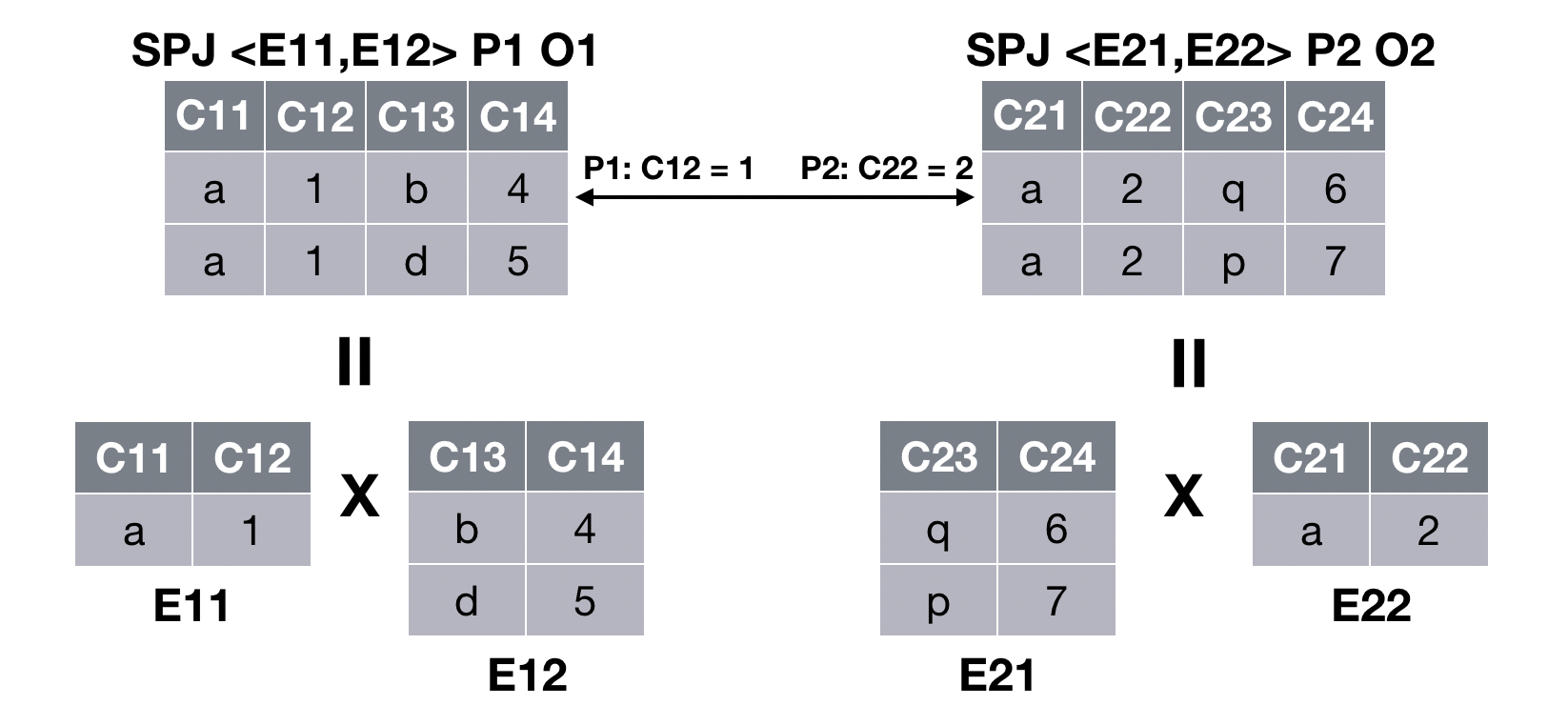
Figure 4: SPJ Queries – Cardinally equivalent SPJ Queries.

Consider the cardinally equivalent SPJ queries shown in Figure 4. In this case, VeriSPJ first verifies that sub-query $E11$ is cardinally equivalent to sub-query $E22$, and sub-query $E12$ is cardinally equivalent to sub-query $E21$. Thus, the two intermediate join tables (i.e., cartesian product of sub-tables) are cardinally equivalent. VeriSPJ constructs two symbolic tuples to represent the bijective map between these intermediate join tables by leveraging the two bijective maps between the underlying tables. VeriSPJ then verifies that two corresponding tuples in the map either both satisfy the predicate or do not satisfy the predicate. Thus, the bijective map between the tuples in the intermediate join tables is the bijective map between the tuples in the output tables before projection.

QPSR: Since VeriSPJ verifies that the given pair of SPJ queries are cardinally equivalent, the two symbolic tuples $\vec{\texttt{{COLS}}_{\_}1}$ and $\vec{\texttt{{COLS}}_{\_}2}$ define a bijective map between tuples in the output tables before projection. Projection does not change the bijective map between tuples as it is applied separately on each tuple. Thus, VeriSPJ leverages ConstExpr to construct new symbolic tuples $\vec{\texttt{{COLS}}^{\prime}_{\_}1}$ and $\vec{\texttt{{COLS}}^{\prime}_{\_}2}$ based on the vector of projection expressions and the given symbolic tuples. The QPSR consists of the derived symbolic tuples $\vec{\texttt{{COLS}}^{\prime}_{\_}1}$, $\vec{\texttt{{COLS}}^{\prime}_{\_}2}$, the conjunction of $\texttt{{COND}}_{\_}1$, $\texttt{{COND}}_{\_}2$ and COND, and the conjunction of all the relational constraints.

Properties: VeriSPJ is sound. Based on 5.6, if VeriSPJ returns the QPSR, then the given SPJ queries are cardinally equivalent. We present a formal proof in § C.2.2.

In general, VeriSPJ is not complete. The reasons are threefold. First, the SMT solver is only complete for linear operators. If the predicates have non-linear operators (e.g., multiplication between columns), then the solver may return UNKNOWN when it should return UNSAT [50]. Second, SPES encodes all user-defined functions, string operations, and higher-order predicates as uninterpreted functions. These encodings do not preserve the semantics of these operations. Third, VeriCard is not complete (§ 5.3).

VeriSPJ procedure is complete if all input queries for the given two SPJ queries are table queries, and the SMT solver can determine the satisfiability of the predicates. This is because the problem of deciding equivalence of two conjunctive (i.e., SPJ) queries is decidable [26].

Lemma 5.7.

For a given pair of cardinally equivalent SPJ queries $\textsc{SPJ}(\vec{e_{\_}1},p_{\_}1,\vec{o_{\_}1})$ and $\textsc{SPJ}(\vec{e_{\_}2},p_{\_}2,\vec{o_{\_}2})$, if $\vec{e_{\_}1}$ and $\vec{e_{\_}1}$ only have table sub-queries, and the SMT solver can determine the satisfiability of the predicates and projection expressions, then VeriSPJ procedure returns the QPSR.

Proof 5.8.

We prove this theorem using the method of contraposition. If VeriSPJ returns NULL, then there are two cases:

Case 1: There is no bijective map between $\overrightarrow{e_{\_}1}$ and $\overrightarrow{e_{\_}2}$, such that each pair of table sub-queries are cardinally equivalent. There are two possible sub-cases.

In the first sub-case, $\overrightarrow{e_{\_}1}$ has more input table queries than $\overrightarrow{e_{\_}2}$. Here, we can always construct the input such that the intermediate join table of $\vec{e_{\_}1}$ has more tuples than the intermediate join table of $\vec{e_{\_}2}$. SPES has eliminated the case where the predicates are $False$ (§ 4.2). Thus, the constructed tuples in intermediate join table can all satisfy the predicate. So, the number of tuples returned by the two SPJ queries is different, and are hence not cardinally equivalent.

In the second sub-case, $\overrightarrow{e_{\_}1}$ have different table queries than $\overrightarrow{e_{\_}2}$. Here, each input table in $\overrightarrow{e_{\_}2}$ contains only one tuple. And a different table in $\overrightarrow{e_{\_}1}$ has two tuples that satisfy the predicate. So, the number of tuples returned by the two SPJ queries is different, and are hence not cardinally equivalent.

Case 2: VeriSPJ cannot verify that the two predicates always return the same result for two corresponding tuples in a bijective map between tuples in the intermediate table. In this case, since both predicates are decidable, the solver will generate a model $m$ such that one symbolic tuple satisfies the predicate and the other one does not. We then construct inputs such that each intermediate table only contains one tuple that matches the values in $m$. Then the first SPJ query returns a table that contains one tuple, while the other one returns an empty table. Thus, the two SPJ queries are not cardinally equivalent.

5.6 Aggregate Queries

Input : A pair of aggregate queries

Output : QPSR of given aggregate queries or NULL

1 Procedure $\textsf{VeriAgg}(\textsc{Agg}(e_{\_}1,~{}\vec{g_{\_}1},~{}\vec{agg_{\_}1}),\textsc{Agg}(e_{\_}2,~{}\vec{g_{\_}2},~{}\vec{agg_{\_}2}))$

2       $QPSR\leftarrow\textsf{VeriCard}(e_{\_}1,e_{\_}2)$

3       if QPSR != NULL  then

4             $(\vec{\texttt{{COLS}}_{\_}1},\vec{\texttt{{COLS}}_{\_}2},\texttt{{COND}},\texttt{{ASSIGN}})\leftarrow QPSR$

5             if $\vec{g_{\_}1}\leftrightarrow\vec{g_{\_}2}$  then

6                   $\vec{\texttt{{COLS}}_{\_}1}\leftarrow\textsf{InitAgg}(\vec{agg_{\_}1})$ :: $\vec{g_{\_}1}$

7                   $\vec{\texttt{{COLS}}_{\_}2}\leftarrow\textsf{CtrAgg}(\vec{agg_{\_}1},\vec{\texttt{{COLS}}_{\_}1},\vec{agg_{\_}2})$ :: $\vec{g_{\_}2}$

8                   return ($\vec{\texttt{{COLS}}_{\_}1},\vec{\texttt{{COLS}}_{\_}2},\texttt{{COND}},\texttt{{ASSIGN}}$)

9             end if

10            

11       end if

12      else return NULL;

13      

14

Algorithm 4 Verification Algorithm for Aggregate Queries

Alg. 4 illustrates the VeriAgg procedure for aggregate queries. If this procedure determines that the two input aggregate queries $\textsc{Agg}(e_{\_}1,~{}\vec{g_{\_}1},~{}\vec{agg_{\_}1})$ and $\textsc{Agg}(e_{\_}2,~{}\vec{g_{\_}2},~{}\vec{agg_{\_}2})$ are cardinally equivalent, then it returns their QPSR. Otherwise, it returns NULL.

Cardinal Equivalence: An aggregate query groups the tuples in the input table based on the GROUP BY column set, and then returns a tuple by applying the aggregate function on each group.

Lemma 5.9.

Two aggregate queries $\textsc{Agg}(e_{\_}1,~{}\vec{g_{\_}1},~{}\vec{agg_{\_}1})$ and $\textsc{Agg}(e_{\_}2,~{}\vec{g_{\_}2},~{}\vec{agg_{\_}2})$ are cardinally equivalent if two conditions are satisfied: (1) the two input sub-queries $e_{\_}1$ and $e_{\_}2$ are cardinally equivalent; (2) for any two pairs of corresponding tuples in a bijective map of the QPSR of $e_{\_}1$ and $e_{\_}2$, two tuples in $e_{\_}1$ belong to the same group as defined by $g_{\_}1$ iff their associated tuples in $e_{\_}2$ belong to the same group as defined by $g_{\_}2$.

VeriAgg first recursively invokes the VeriCard procedure to determine the cardinal equivalence of the two input sub-queries $e_{\_}1$ and $e_{\_}2$ (Alg. 4). If VeriCard returns the QPSR of $e_{\_}1$ and $e_{\_}2$, then VeriAgg has proved the first condition in 5.9.

To prove the second condition, VeriAgg collects the symbolic tuples $\vec{\texttt{{COLS}}_{\_}1}$ and $\vec{\texttt{{COLS}}_{\_}2}$ from the QPSR. Since these two symbolic tuples represent a bijective map between tuples returned by $e_{\_}1$ and $e_{\_}2$, VeriAgg replaces all variables in $\vec{\texttt{{COLS}}_{\_}1}$ and $\vec{\texttt{{COLS}}_{\_}2}$ by a set of fresh variables to generate a second pair of symbolic tuples $\vec{\texttt{{COLS}}^{\prime}_{\_}1}$ and $\vec{\texttt{{COLS}}^{\prime}_{\_}2}$ that represents the same bijective map with different tuples.

We decompose the proof for the second condition into two stages (Alg. 4). In the first stage, we want to prove that if $\vec{\texttt{{COLS}}_{\_}1}$ and $\vec{\texttt{{COLS}}^{\prime}_{\_}1}$ belong to the same group, then $\vec{\texttt{{COLS}}_{\_}2}$ and $\vec{\texttt{{COLS}}^{\prime}_{\_}2}$ also belong to the same group. To prove this, VeriAgg extracts the GROUP BY column sets $\vec{g_{\_}1}$, $\vec{g^{\prime}_{\_}1}$, $\vec{g_{\_}2}$ and $\vec{g^{\prime}_{\_}2}$ from $\vec{\texttt{{COLS}}_{\_}1}$, $\vec{\texttt{{COLS}}^{\prime}_{\_}1}$, $\vec{\texttt{{COLS}}_{\_}2}$ and $\vec{\texttt{{COLS}}^{\prime}_{\_}2}$, respectively. It then attempts to prove the property:

$$(\texttt{{COND}}\land\texttt{{ASSIGN}}\land\vec{g_{\_}1}=\vec{g^{\prime}_{\_}1})\implies\vec{g_{\_}2}=\vec{g^{\prime}_{\_}2}$$

VeriAgg sends the negation of this property to the solver. If the solver decides that this formula is unsatisfiable, then it is impossible to find two tuples returned by $e_{\_}1$ that are assigned to the same group by $\vec{g_{\_}1}$, such that their corresponding tuples returned by $e_{\_}2$ are assigned to different groups by $\vec{g_{\_}2}$. In the second stage, we use the same technique in the reverse direction of the implication.

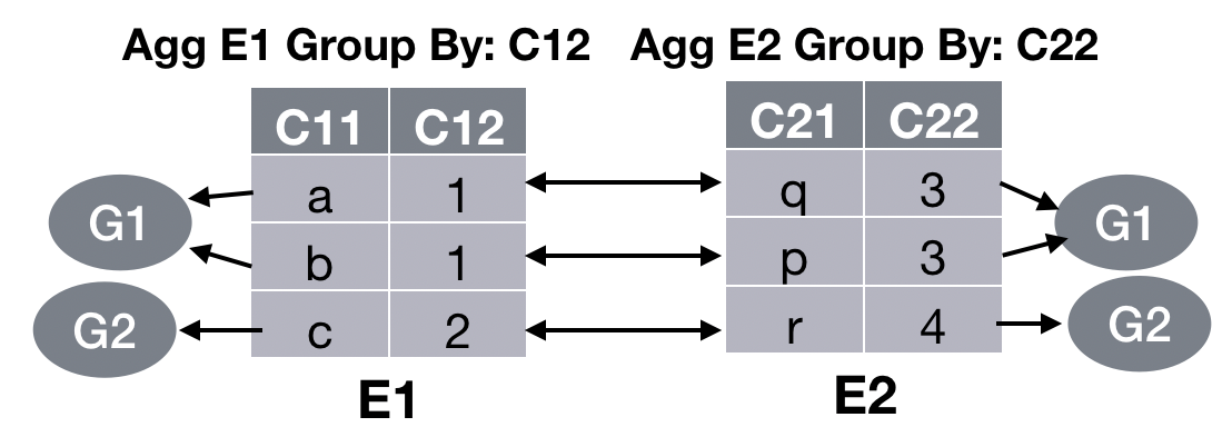
Figure 5: Aggregate Queries – Cardinally equivalent aggregate queries.

Consider the cardinally equivalent aggregate queries shown in Figure 5. VeriAgg first verifies that the two input queries $E1$ and $E2$ are cardinally equivalent, and then constructs the QPSR to represent the bijective map between their returned tuples. VeriAgg then verifies that if two arbitrary tuples in $E1$ belong to same group (e.g., first two tuples), then the two corresponding tuples in $E2$ also belong to the same group. It also verifies that if two arbitrary tuples in $E1$ belong to different groups (e.g., first and third tuples), then the two corresponding tuples in $E2$ also belong to different groups. VeriAgg verifies two aggregate queries are cardinally equivalent by verifying that they emit the same number of groups.

QPSR: VeriAgg constructs the QPSR of two given aggregate queries after proving they are cardinally equivalent. $\vec{\texttt{{COLS}}_{\_}1}$ and $\vec{\texttt{{COLS}}_{\_}2}$ define a bijective map between tuples returned by input queries, and can also be used to define a bijective map between groups in two aggregate queries. If two aggregate functions in $\vec{agg_{\_}1}$ and $\vec{agg_{\_}2}$ are the same and operate on same values (i.e., input columns of the symbolic tuples are the same), then the aggregate values in the output tuples are the same, since each group contains the same number of tuples.

VeriAgg invokes the InitAgg procedure on $\vec{agg_{\_}1}$ to construct a vector of pairs of new symbolic variables as the symbolic tuples for aggregate functions. In each pair of symbolic variables, the first variable represents the aggregate value. The second variable indicates if the aggregate value is NULL. VeriAgg concatenates the GROUP BY column set $\vec{g_{\_}1}$ with the symbolic tuple $\vec{\texttt{{COLS}}_{\_}1}$. VeriAgg then invokes the CtrAgg procedure to construct the symbolic columns for $\vec{agg_{\_}2}$, and then concatenates with the GROUP BY column set $\vec{g_{\_}2}$. CtrAgg uses the same pairs of symbolic variables for all aggregation operations in $\vec{agg_{\_}2}$, where the aggregation function type and operand columns are the same in $\vec{agg_{\_}1}$. VeriAgg propagates COND and ASSIGN into the sub-QPSRs.

Properties: VeriAgg is sound. Based on 5.9, if VeriAgg returns the QPSR, then the two given aggregate queries are cardinally equivalent. This is because the two symbolic tuples $\vec{\texttt{{COLS}}_{\_}1}$ and $\vec{\texttt{{COLS}}_{\_}2}$ are constructed from corresponding groups. Thus, $\vec{\texttt{{COLS}}_{\_}1}$ and $\vec{\texttt{{COLS}}_{\_}2}$ define a bijective map between tuples returned by the two aggregate queries. We present a formal proof in Section C.2.3.

VeriAgg is not complete. The sources of incompleteness are threefold: (1) incompleteness of VeriCard, (2) limitations of the SMT solver, and (3) when VeriCard returns the QPSR of two input sub-queries, the symbolic tuples in the QPSR define only one possible bijective map between tuples in the input tables. If VeriAgg fails to prove the second condition in 5.9, it is still possible that there exists another bijective map that satisfies the second condition.

5.7 Union Queries

Input : A pair of union queries

Output : QPSR of given two union queries or NULL

1 Procedure $\textsf{VeriUnion}(\textsc{Union}(\vec{e_{\_}1}),\textsc{Union}(\vec{e_{\_}2}))$

2       $\{\vec{QPSR}\}\leftarrow\textsf{VeriVec}(\vec{e_{\_}1},\vec{e_{\_}2})$

3       if $\{\vec{QPSR}\}$ != $\emptyset$  then

4             $\vec{\texttt{{COLS}}_{\_}1}\leftarrow\textsf{InitTuple}()$; $\vec{\texttt{{COLS}}_{\_}2}\leftarrow\textsf{InitTuple}()$

5             $\vec{QPSR}\leftarrow\{\vec{QPSR}\}$

6             $(\texttt{{COND}},\texttt{{ASSIGN}})\leftarrow\textsf{ConstAssign}(\vec{QPSR},\vec{\texttt{{COLS}}_{\_}1},\vec{\texttt{{COLS}}_{\_}2})$

7             return ($\vec{\texttt{{COLS}}_{\_}1},\vec{\texttt{{COLS}}_{\_}2},\texttt{{COND}},\texttt{{ASSIGN}}$)

8       end if

9      else return NULL;

10      

11

Algorithm 5 Verification Algorithm for Union queries

Alg. 5 illustrates the VeriUnion procedure for union queries. If it determines that the union expressions are cardinally equivalent, then it returns their QPSR. Otherwise, it returns NULL.

Lemma 5.10.

Two union queries $\textsc{Union}(\vec{e_{\_}1})$ and $\textsc{Union}(\vec{e_{\_}2})$ are cardinally equivalent if there exists a bijective map between the two input sub-queries $\vec{e_{\_}1}$ and $\vec{e_{\_}2}$, such that each pair of queries are cardinally equivalent.

Cardinal Equivalence: The lemma directly follows from the semantics of the union queries. VeriUnion procedure invokes VeriVec (§ 5.5) to find a bijective map between $\vec{e_{\_}1}$ and $\vec{e_{\_}2}$ (Alg. 5), such that each pair of queries are cardinally equivalent.

QPSR: VeriVec finds all candidate bijective maps ($\{\vec{QPSR}\}$) between two input sub-queries $\vec{e_{\_}1}$ and $\vec{e_{\_}2}$, such that each pair of sub-queries are cardinally equivalent. In each candidate bijective map ($\vec{QPSR}$), a vector of QPSRs is constructed such that each QPSR defines a bijective map between tuples returned by a pair of sub-queries. VeriUnion gets an arbitrary $\vec{QPSR}$ (i.e., one candidate bijective map between the sub-queries). It seeks to construct a bijective map between tuples returned by two union queries that preserves all of the bijective maps between tuples returned by sub-queries in that $\vec{QPSR}$. It first constructs two fresh symbolic tuples $\vec{\texttt{{COLS}}_{\_}1}$ and $\vec{\texttt{{COLS}}_{\_}2}$. It then invokes the ConstAssign procedure to set ASSIGN such that both $\vec{\texttt{{COLS}}_{\_}1}$ and $\vec{\texttt{{COLS}}_{\_}2}$ are always equivalent to the symbolic tuples in one sub-QPSR returned by VeriVec, and COND such that COND in one sub-QPSR holds when symbolic tuples equal to the tuples in that sub-QPSR. ConstAssign creates a vector of boolean variables to set these constraints. VeriUnion returns these two symbolic tuples, COND, and ASSIGN as the QPSR of the given union queries.

Properties: VeriUnion is sound. Based on 5.10, if VeriUnion returns the QPSR, then the two union queries are cardinally equivalent. The symbolic tuples $\vec{\texttt{{COLS}}_{\_}1}$ and $\vec{\texttt{{COLS}}_{\_}2}$ define a bijective map between tuples returned by two union queries that preserves all of the bijective maps between tuples in their cardinally equivalent sub-queries. The formal proof is given in § C.2.4.

VeriUnion is incomplete. The sources of incompleteness are threefold: (1) incompleteness of VeriCard, (2) limitations of the SMT solver, and (3) two union queries may be cardinally equivalent even if there is no bijective map between their sub-queries such that each pair of sub-queries is cardinally equivalent.

6 Soundness and Completeness

We now discuss the soundness and completeness of SPES for verifying the equivalence of two queries.

Soundness: SPES is sound.

Lemma 6.11.

Given a pair of queries Q1 and Q2, if VeriCard returns a QPSR of Q1 and Q2, then Q1 and Q2 are cardinally equivalent and the pair of symbolic tuples $(\vec{\texttt{{COLS}}_{\_}1},\vec{\texttt{{COLS}}_{\_}2})$ symbolically represents a bijective map between tuples returned by Q1 and Q2.

Proof 6.12.

Proof is by induction on Q1 (the choice of Q1 versus Q2 is arbitrary). Each case on the form Q1 is proved by the soundness of four sub-procedure and the inductive hypothesis in cases when Q1 is composite of sub-queries.

Lemma 6.13.

Given two queries Q1 and Q2, if SPES constructs the QPSR of two normalized queries, and checks the formula holds for the QPSR: $\texttt{{COND}}\land\texttt{{ASSIGN}}\implies\vec{\texttt{{COLS}}_{\_}1}=\vec{\texttt{{COLS}}_{\_}2}$ then Q1 and Q2 are fully equivalent.

Proof 6.14.

Based on 6.11, if SPES constructs the QPSR, then $\vec{\texttt{{COLS}}_{\_}1}$ and $\vec{\texttt{{COLS}}_{\_}2}$ symbolically represents a bijective map between tuples returned by cardinally equivalent Q1 and Q2. Thus, Q1 and Q2 are fully equivalent based on 5.3.

Completeness: In general, SPES is not complete. Sources of incompleteness are discussed in Sections 5.3, 5.4, 5.5, 5.6 and 5.7, and discuss their practical impact in § 7.4. However, SPES is complete for a pair of SPJ queries Q1 and Q2 that do not have predicates or projection expressions whose satisfiability cannot be determined by the SMT solver and the input sub-queries are only table queries.

Proof 6.15.

Based on 5.7, if Q1 and Q2 are fully equivalent, then VeriCard returns an QPSR. Based on 6.11, $\vec{\texttt{{COLS}}_{\_}1}$ and $\vec{\texttt{{COLS}}_{\_}2}$ symbolically represent the bijective map between tuples returned by Q1 and Q2 for all valid inputs. Since Q1 and Q2 do not have predicates and projection expressions whose satisfiability cannot be determined by the SMT solver, If the SMT solver determines $\texttt{{COND}}\land\texttt{{ASSIGN}}\land\neg(\vec{\texttt{{COLS}}_{\_}1}=\vec{\texttt{{COLS}}_{\_}2})$ is satisfiable, then it generates a model $m$. The model $m$ defines input tables from which Q1 and Q2 each return non-identical tuples equal to the interpretation of their respective symbolic tuples under $m$. Thus, Q1 and Q2 are not fully equivalent. By contradiction, SPES is complete.

7 Evaluation

In this section, we describe our implementation and evaluation of SPES. We begin with a description of our implementation in § 7.1. We next report the results of a comparative analysis of SPES against EQUITAS [50] and UDP [23], state-of-the-art automated QE verifiers based on SR and AR, respectively. We then quantify the efficacy of SPES in identifying overlapping queries across production SQL queries in § 7.3. We conclude with the limitations of the current implementation of SPES in § 7.4.

QE Verifier	Supported Semantics	Supported Pairs	Proved Pairs	Average Time (s)	USPJ Pairs	Average Time (s)	Aggregate Pairs	Average Time (s)	Outer-Join Pairs	Average Time (s)
EQUITAS	Set	91	67	0.15	28	0.10	32	0.19	9	0.19
UDP	Bag	39	34	N/A	21	N/A	11	N/A	–	–
SPES (w/o norm.)	Bag	120	56	0.02	31	0.01	24	0.04	3	0.1
SPES	Bag	120	95	0.05	42	0.05	44	0.06	20	0.08

Table 1: Comparative analysis between SPES, EQUITAS, and UDP - The results include the number of query pairs in the Calcite benchmark that these tools support, the number of pairs whose equivalence they can prove, and the average time they take to determine QE.

7.1 Implementation

Figure 6: Query Equivalence Verification Pipeline - The pipeline for determining the equivalence of SQL queries.

The architecture of SPES is illustrated in Figure 6. SPES takes a pair of SQL queries as inputs and returns a boolean decision that indicates whether they are fully equivalent. The QE verification pipeline consists of three components: ❶ The compiler converts the given queries to logical query execution plans. We use the open-sourced Calcite framework [3]. ❷ SPES operates on these logical plans in two stages. First, it converts them to the categories of queries that it supports and normalizes them. Next, it uses the third component (i.e., an SMT solver) to verify the cardinal equivalence of two queries and then constructs their QPSR. It also uses the solver for verifying the properties of QPSR to determine full equivalence. We implement this component in Java (2,065 lines of code). ❸ The third component is an SMT solver Z3 that SPES leverages for determining the satisfiability of FOL formulae [12]. We have published the source code of SPES on GitHub [spes].

7.2 Comparative Analysis

Comparison Tools: We compare SPES against two QE verifiers: EQUITAS [50] and UDP [23]. EQUITAS takes a symbolic approach and only supports set semantics. UDP takes an algebraic approach and does support bag semantics.

Benchmark: We use queries in the test suite of Apache Calcite [3] as our benchmark. This test suite contains 232 semantically equivalent query pairs. The reasons for using this benchmark are twofold. First, the Calcite optimizer is widely used in data processing engines [4, 5, 6, 7, 8]. So, it covers a wide range of SQL features. Second, since EQUITAS and UDP are both evaluated on this query pair benchmark [23, 50], we can quantitatively and qualitatively compare the efficacy of these tools. We send every query pair with the schemata of their input tables to SPES and ask it to check their QE. We conduct this experiment on a commodity server (Intel Core i7-860 processor and 16 GB RAM).

Automated SQL QE Verifiers: The results of this experiment are shown in Table 1. We compare SPES against EQUITAS in the same environment. We present the results reported in the UDP paper [23].

We evaluate SPES under two configurations to delineate the impact of the normalization rules. ❶ SPES (w/o normalization) naively converts the original queries to a tree representation without normalizing them, and then applies the verification algorithms. ❷ SPES additionally leverages a minimal set of normalization rules.

SPES proves the equivalence of a larger set of query pairs (95/232) compared to UDP (34/232) and EQUITAS (67/232). SPES currently supports 120 out of 232 pairs. The un-supported queries either: (1) contain SQL features that are not yet supported (e.g., CAST), or (2) cannot be compiled by Calcite due to syntax errors. Among the 120 pairs supported by SPES, it proves that 95 pairs (80%) are equivalent under bag semantics. In contrast, UDP proves the equivalence of 34 pairs under bag semantics. EQUITAS proves the equivalence of 67 pairs, but only under set semantics. We group the proved query pairs into three categories:

• USPJ: Queries that are union of SELECT-PROJECT-JOIN.

• Aggregate: Queries containing at least one aggregate.

• Outer-Join: Queries containing at least one outer JOIN.

Table 1 reports the number of pairs proved by UDP and EQUITAS in each category. The number of proved pairs containing outer JOIN is not known in case of UDP. SPES outperforms the other tools on queries containing aggregate and outer JOIN operators. SPES proves QE of a larger set of query pairs (95/232) compared to SPES (w/o normalization) (56/232). This illustrates the importance of the normalization stage of SPES for real-world applications.

Efficiency: We next compare the average time taken by SPES and EQUITAS to prove the equivalence of a pair of queries in each category. This is an important metric for a cloud-scale tool that must be deployed in a DBaaS platform. We only compute this metric for the pairs that these tools can prove. SPES and EQUITAS take 0.05 s and 0.15 s on average to prove QE, respectively. So, SPES is 3$\times$ faster than EQUITAS on this benchmark. SPES consistently outperforms EQUITAS across all categories of queries.

Query Set	Number of Queries	Queries with Overlapping Computation	Highest Query Frequency	Compared Query Pairs	Equivalent Query Pairs	Equivalent Pairs with Aggregate and Join
Set 1	3285	943	52	122900	3344	653
Set 2	3633	984	97	55311	7225	4822
Set 3	2568	664	30	15442	1521	356
Total	9486	2591 (27%)	–	193633	12090	5831 (48%)

Table 2: Efficacy of SPES on Production Queries - "Highest Query Frequency" indicates the highest frequency of a query in equivalent query pairs. “Compared Query Pairs" refers to number of query pairs that operate on the same set of input tables.

7.3 Efficacy on Production Queries

In this experiment, we quantify the efficacy of SPES in detecting overlap in production SQL queries. We leverage three sets of real production queries from Ant Financial [2], a financial technology company. These queries are used to detect fraud in business transactions. In each set, we run SPES on each pair of queries that operate on the same set of input tables. If SPES decides that a given pair of queries are not equivalent, then we check any constituent sub-queries that operate on the same input tables. We skip checking queries containing only table scans and those that only differ in the parameters passed on to their predicates. This is because SPES trivially proves their equivalence and the computational resources needed for evaluating such queries are negligible.

Table 2 presents the results of this experiment. SPES effectively identifies overlap between complex analytical queries. Among 9486 queries, SPES finds overlapping computation between 2591 (27%) queries, while EQUITAS only finds overlapping computation between 1126 (12%) queries. These tools report overlapping computation if the query or a constituent sub-query is equivalent to another query or sub-query within the set.

We also report the highest frequency of queries present in these pairs that are repeatedly executed in the workload. In practice, most of the computational resources are expended on executing queries containing aggregate functions or different types of join. Among 12090 equivalent pairs, 5831 (48%) contain join and aggregate operations. This illustrates that SPES works well on queries containing these operators.

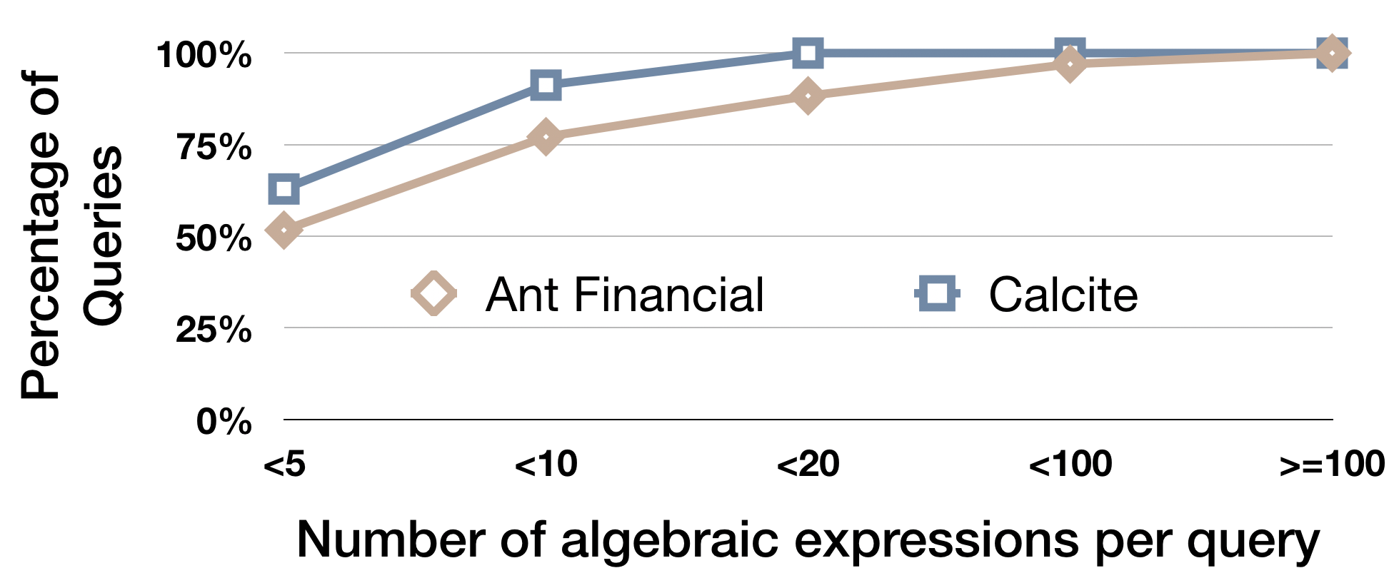
Figure 7: Complexity of Production Queries - We quantify the complexity of production queries in the Ant Financial workload by measuring the number of sub-queries in each query.

Query Complexity: Figure 7 illustrates the complexity of queries in this workload. We compute the distribution of the number of sub-queries in a given query (complex queries will have a larger set of sub-queries). We found that the average number of algebraic expressions in the Ant Financial workload (45.38) is 8$\times$ larger than that in the Calcite benchmark (5.37).

7.4 Limitations

In general, the problem of deciding QE is undecidable [15]. Among the 120 query pairs supported by SPES, it cannot prove the QE of 25 pairs. We classify them into three categories: (1) lack of normalization rules ($21$), and (2) support for additional integrity constraints ($4$)

Normalization Rules: SPES verifies the cardinal equivalence of two queries only if it is able to normalize them into the same type of queries using a set of pre-defined semantically-equivalent rewrite rules (§ 5.3). We will need to introduce additional normalization rules for queries with: (1) union and aggregate (15/21), and (2) join and aggregate (6/21), Adding these rewrite rules in the normalization stage will enable SPES to prove the QE of these 21 pairs. However, it will also increase the average QE verification time. Furthermore, these rules are not required for supporting production queries discussed in § 7.3.

Integrity Constraints: SPES currently only has partial support for integrity constraints in the form of normalization rules (§ 4.2): (1) self join on primary key, and (2) grouping based on primary key. We plan to add additional rules to handle join on primary and foreign keys in the future. For example, we may normalize an OUTER JOIN operation based on a foreign key to an INNER JOIN operation.

8 Related Work

Query Equivalence: The state-of-the-art QE verification tools are based on either symbolic reasoning [50] or algebraic reasoning [24, 22, 25] . Tools based on algebraic representation include COSETTE and UDP that rely on $\mathcal{K}$-relation and $\mathcal{U}$-semi-ring theories, respectively. Tools based on symbolic reasoning include EQUITAS. We highlighted the differences between SPES and these tools in § 2.

Prior efforts have examined the theoretical aspects of equivalence and containment relationships between queries. Since it is an undecidable problem [14, 18], these efforts focused on determining categories of queries for which it is a decidable problem: (1) conjunctive queries [21], (2) conjunctive queries with additional constraints [19, 36, 28], and (3) conjunctive queries under bag semantics [37]. The problem of deciding the containment relationship between conjunctive queries can be reduced to a constraint satisfiability problem [40]. Other proposals include decision procedures for proving the equivalence of a subset of queries under set [20, 45, 44] and bag semantics [27, 31, 32, 42]. There is a large body of work on optimizing queries using materialized views [33, 43, 17, luis2014, sanjay2000]. These systems internally use a QE verification algorithm that relies on syntactical equivalence and that work on a subset of SQL queries. These systems may leverage SPES to better detect QE and deliver more optimized execution plans.

Symbolic Reasoning in DBMSs: Researchers have leveraged symbolic reasoning in DBMSs by reducing the given problem to an FOL satisfiability problem and then using an SMT solver to solve it. These efforts include: (1) automatically generating test cases for database applications [46, 47, 13], (2) verifying the correctness of database applications [48, 38, 34], (3) disproving the equivalence of SQL queries [24], and (4) finding the best application-aware memory layout [49]. SPES differs from these efforts in that it uses symbolic reasoning to prove QE under bag semantics.

9 Conclusion

In this paper, we presented the design and implementation of SPES, an automated tool for proving query equivalence under bag semantics using symbolic reasoning. We reduced the problem of proving equivalence under bag semantics to that of proving the existence of a bijective, identity map between the output tables of the queries for all valid input tables. SPES classifies queries into four categories, and leverages a set of category-specific verification algorithms to effectively determine their equivalence. Our evaluation shows that SPES proves the equivalence of a larger set of query pairs under bag semantics compared to state-of-the-art tools based on symbolic and algebraic approaches. Furthermore, it is 3$\times$ faster than EQUITAS that only proves equivalence under set semantics.

Appendix A Semantics of AR

We now formally define the semantics of queries, using the following formal notation. $\Downarrow$ is the evaluation symbol. The left side of this symbol is an algebraic expression that is evaluated on valid input tables Ts. The right side of this symbol is the evaluation result, which is the output table. All output tables are bags (i.e., can contain duplicate tuples). A horizontal line separates the pre- and the post-conditions. The pre-conditions on the top of the line include a set of evaluation relations. The post-condition on the bottom side of the line is an evaluation relation. If all the relations in the pre-conditions hold, then the relation in the post-condition holds.

$$\inference[ ]{}{\langle\textsc{Table}(n)[\texttt{Ts}]\rangle\Downarrow[t|\forall t\in n]}$$E-Table

$$\inference[ ]{\langle\textsf{e}[\texttt{Ts}]\rangle\Downarrow T_{\_}0}{\langle\textsc{Agg}(\textsf{e},~{}\vec{g},~{}\vec{agg})[\texttt{Ts}]\rangle\Downarrow[\vec{agg}(t)|\forall t\in part(T_{\_}0,\vec{g})]}$$E-Agg

Figure 8: Semantics – Semantics of queries used in SPES

• Given a set of valid input tables Ts, the table query returns all the tuples in table $n$.

• Given a set of valid input tables Ts, the SPJ query first evaluates the vector of input sub-queries on Ts to obtain a vector of input tables. For each tuple $t$ in the cartesian product of the vector of input tables, if $t$ satisfies the given predicate $p$, it then applies the vector of expressions $\overrightarrow{o}$ on the selected tuple $t$ and emits the transformed tuple.

• Given a set of valid input tables Ts, this aggregate query first evaluates the input sub-query on Ts to get an input table $T_{\_}0$. Then, it uses part to partition the input table $T_{\_}0$ into a set of bags of tuples as defined by a set of group set $\vec{g}$ (tuples in each bag take the same values for the grouping attributes). Lastly, for each bag of tuples, it applies the vector of aggregate functions and returns one tuple.

• Given a set of valid input tables Ts, this union query first evaluates the vector of input sub-queries on Ts to get a vector of input tables. It then returns all the tuples present in the input tables, which does not eliminate duplicate tuples.

Appendix B Predicate & Proj. Expression

SPES supports the predicate and project expressions shown in Figure 9. It uses the same encoding scheme as the one employed in EQUITAS (described in Section 3.4 of [50]).

$$\mathsf{E}::=\mathsf{Column}~{}i|\mathsf{Const}~{}v|\texttt{{NULL}}|\mathsf{Bin}~{}\mathsf{E}~{}\mathsf{OP}~{}\mathsf{E}|\mathsf{Fun}~{}N~{}(\overrightarrow{\mathsf{E}})|\mathsf{CASE}~{}$$ (1)

$$\mathsf{CASE}~{}::=\mathsf{Pair}~{}\mathsf{E}$$ (2)

$$\mathsf{Pair}~{}::=(\mathsf{WHEN}~{}\mathsf{P}~{}\mathsf{E})\mathsf{Pair}~{}|\epsilon$$ (3)

$$\mathsf{OP}::=+|-|\times|\div|mod$$ (4)

$$\mathsf{P}::=\mathsf{BinE}~{}\mathsf{E}~{}\mathsf{CP}~{}\mathsf{E}|\mathsf{BinL}~{}\mathsf{P}~{}\mathsf{LOGIC}~{}\mathsf{P}|\mathbf{Not}~{}\mathsf{P}|\mathbf{IsNull}~{}\mathsf{E}$$ (5)

$$\mathsf{CP}::=~{}>|<|=|\leq|\geq$$ (6)

$$\mathsf{LOGIC}::=~{}\texttt{{AND}}|~{}\texttt{{OR}}$$ (7)

Figure 9: Predicate & Projection Expressions – Types of predicates and projection expressions supported by SPES.

A projection expression $\mathsf{E}$ can either be a column that refer to a specific column, a constant value, NULL, a binary expression, an uninterpreted function, or an CASE expression (Eqn. 1). A predicate $\mathsf{P}$ can either be a binary comparison between two projection expression, a binary predicate that is composed by two predicates, a not predicate and a predicate decide if a projection expression is NULL (Eqn. 5).

Appendix C Soundness of Verification

In this section, we give the formal proof of the soundness of SPES. The overall proof is structured as follows: we introduce symbolic representations of bijections over tuples in (§ C.1), prove correctness of the procedure for generating symbolic representations (§ C.2), and then prove correctness of the procedure for determining equivalence (§ C.3).

C.1 Symbolic bijections between queries

All definitions in this section are given with respect to arbitrary queries Q1 and Q2, whose columns are denoted $\vec{\texttt{{COLS}}_{\_}1}$ and $\vec{\texttt{{COLS}}_{\_}2}$, respectively.

A cardinality-preserving binary relation between Q1 and Q2 is a relation

$$R\subseteq\vec{\texttt{{COLS}}_{\_}1}\times\vec{\texttt{{COLS}}_{\_}2}$$

such that for each input table set $I$ and all tuples $(t,u)\in R$, it holds that

$$|t|_{\texttt{Q1}(I)}=|u|_{\texttt{Q2}(I)}$$

where $|u|_{T}$ denotes the number of occurrences of tuple $u$ in table $T$.

Cardinality-preserving binary relations can act as witnesses of full equivalence (see 2) between queries.

Lemma C.16.

If the identity function is a cardinality-preserving binary relation between Q1 and Q2, then Q1 and Q2 are fully equivalent (denoted $\texttt{Q1}\equiv\texttt{Q2}$).

Proof C.17.

Let $I$ be an arbitrary table set and let $t$ be an arbitrary tuple over columns COLS. Then

$$|t|_{\texttt{Q1}(I)}=|t|_{\texttt{Q2}(I)}$$

by the fact that the identity function is cardinality-preserving. Thus $\texttt{Q1}(I)$ and $\texttt{Q2}(I)$ are equivalent under bag semantics by the definition of bag semantics. Thus $\texttt{Q1}\equiv\texttt{Q2}$, by definition of equivalence.

A symbolic representation of a binary relation

$$R\subseteq\vec{\texttt{{COLS}}_{\_}1}\times\vec{\texttt{{COLS}}_{\_}2}$$

is an SMT formula over a vocabulary that extends $\vec{\texttt{{COLS}}_{\_}1}$ and $\vec{\texttt{{COLS}}_{\_}2}$ such that for each $(t,u)\in R$, there is some model $m$ of $\varphi$ such that

$$t= \ m(\vec{\texttt{{COLS}}_{\_}1}) u= \ m(\vec{\texttt{{COLS}}_{\_}2})$$

where $m(\vec{\texttt{{COLS}}_{\_}1})$ is the tuple of interpretations of each column name in $\vec{\texttt{{COLS}}_{\_}1}$ (and similarly for $m(\vec{\texttt{{COLS}}_{\_}2})$).

Symbolic representations of cardinality-preserving bijections can be viewed as QPSRs (defined in Section 5.2), collapsed into single SMT formulas. In particular each QPSR $(C_{\_}1,C_{\_}2,c,a)$ of Q1 and Q2 corresponds to the symbolic relation

$$\vec{\texttt{{COLS}}_{\_}1}=C_{\_}1\land\vec{\texttt{{COLS}}_{\_}2}=C_{\_}2\land c\land a$$

Symbolic cardinality-preserving bijections can be conjoined with equivalent constraints over column fields to form new symbolic cardinality-preserving bijections. In order to formalize this, we will say that for each partial bijection $b$ between $\vec{\texttt{{COLS}}_{\_}1}$ and $\vec{\texttt{{COLS}}_{\_}2}$, each formula $\varphi_{\_}1$ over vocabulary $\texttt{{COLS}}_{\_}1$, and each formula $\varphi_{\_}2$ over vocabulary $\varphi_{\_}2$, $\varphi_{\_}1$ and $\varphi_{\_}2$ are equivalent over $b$ if $m$ is a model of $\varphi_{\_}1$ if and only if $b(m)$ is a model of $\varphi_{\_}2$.

Lemma C.18.

For each cardinality-preserving bijection $b$ symbolically represented by $\varphi$ and all $\psi_{\_}1$ over $\vec{\texttt{{COLS}}_{\_}1}$ and $\psi_{\_}2$ over $\vec{\texttt{{COLS}}_{\_}2}$ that are equivalent over $b$,

$$\varphi\land\psi_{\_}1\land\psi_{\_}2$$

is a symbolic cardinality-preserving bijection.

Proof C.19.

$b|_{\_}{\iota(\varphi_{\_}1)}$ is is the interpretation of $\varphi\land\psi_{\_}1\land\psi_{\_}2$. It is a cardinality-preserving bijection because it is a restriction of a cardinality-preserving bijection.

Because cardinality-preserving bijections can act as witnesses of equivalence, their symbolic representations naturally can, as well.

Lemma C.20.

If there is some symbolic cardinality-preserving bijection $\varphi$ between Q1 and Q2 that entails

$$\vec{\texttt{{COLS}}_{\_}1}=\vec{\texttt{{COLS}}_{\_}2}$$

then $\texttt{Q1}\equiv\texttt{Q2}$.

Proof C.21.

$\varphi$ represents the identity function by the assumptions that it represents a total function and that it logically entails a symbolic representation of the identity relation. Thus, $\texttt{Q1}\equiv\texttt{Q2}$, by Lemma C.16.

C.2 Synthesizing symbolic bijections

We now prove the soundness of the procedure VeriCard. The proof is defined using a set of lemmas per form of input query (Section C.2.1—Section C.2.4), each of which are predicated on assumptions that VeriCard is sound on smaller queries. The proof for arbitrary queries combines the lemmas that concern each form of query in a proof by induction on VeriCard’s input query (Section C.2.5).

C.2.1 Symbolic bijections between table queries

We now state and prove the soundness of VeriTable, which is given in Algorithm 2. For a given pair of table queries $\textsc{Table}(n_{\_}1)$ and $\textsc{Table}(n_{\_}2)$, VeriTable first checks if two table queries have the same name. If two table queries have the same names, then VeriTable uses procedure InitTuple to create a new vector of pair of symbolic variables based on the input table schema, and assign this new vector to $\vec{\texttt{{COLS}}_{\_}1}$. VeriTable then sets $\vec{\texttt{{COLS}}_{\_}1}$ is equal to $\vec{\texttt{{COLS}}_{\_}2}$. VeriTable returns the QPSR with $\vec{\texttt{{COLS}}_{\_}1}$ and $\vec{\texttt{{COLS}}_{\_}2}$, where both COND and ASSIGN are TRUE. If two table queries have different names, then VeriTable returns NULL.

Lemma C.22.

If VeriTable, given two table queries $q_{\_}1=\textsc{Table}(n_{\_}1)$ and $q_{\_}2=\textsc{Table}(n_{\_}2)$, returns some QPSR $\varphi$, then $\varphi$ is symbolic cardinality-preserving bijection between $q_{\_}1$ and $q_{\_}2$.

Proof C.23.

VeriTable determines that $n_{\_}1=n_{\_}2$, by the fact that VeriTable only returns a QPSR if $n_{\_}1=n_{\_}2$ and by the assumption that VeriTable returns a QPSR. The QPSR returned by VeriTable is the symbolic representation of the identity relation, and is thus a symbolic cardinality-preserving bijection.

C.2.2 Symbolic bijections between SPJ queries

We now formalize and prove the correctness of VeriSPJ (see Section 5.5).

Lemma C.24.

For vectors of queries $\overrightarrow{e_{\_}1}$ and $\overrightarrow{e_{\_}2}$, if $\textsf{VeriCard}(e_{\_}1^{\prime},e_{\_}2^{\prime})$ is an QPSR $\varphi^{\prime}$ only if $\varphi^{\prime}$ is a symbolic cardinality-preserving bijection between $e_{\_}1^{\prime}$ and $e_{\_}2^{\prime}$ for all $e_{\_}1^{\prime}\in\overrightarrow{e_{\_}1}$ and $e_{\_}2^{\prime}\in\overrightarrow{e_{\_}2}$, then then VeriSPJ, given queries $\texttt{Q1}=\textsc{SPJ}(\overrightarrow{e_{\_}1},p_{\_}1,\overrightarrow{o_{\_}1})$ and $\texttt{Q2}=\textsc{SPJ}(\overrightarrow{e_{\_}2},p_{\_}2,\overrightarrow{o_{\_}2})$, returns a QPSR $\varphi$ only if $\varphi$ is a symbolic cardinality-preserving bijection between Q1 and Q2.

Proof C.25.

There is some $\mathsf{QPSR}$ in $\textsf{VeriVec}(\overrightarrow{e_{\_}1},\overrightarrow{e_{\_}2})$, by the definition of VeriSPJ (Algorithm 3, Algorithm 3, Algorithm 3, Algorithm 3, and Algorithm 3) and the semantics of VeriVec. $\mathsf{QPSR}$ represents a symbolic cardinality-preserving bijection $\varphi$ between the Cartesian product of $\overrightarrow{e_{\_}1}$ and the Cartesian product of $\overrightarrow{e_{\_}2}$, by the assumption that $\textsf{VeriCard}(e_{\_}1^{\prime},e_{\_}2^{\prime})$ is a symbolic cardinality-preserving bijection for all $e_{\_}1\in\overrightarrow{e_{\_}1}$ and $e_{\_}2\in\overrightarrow{e_{\_}2}$.

Thus $\varphi\land\texttt{{COND}}_{\_}1\land\texttt{{COND}}_{\_}2$ is a symbolic cardinality-preserving bijection by Lemma C.18 applied to $\texttt{{COND}}_{\_}1$ and $\texttt{{COND}}_{\_}2$ and the definition of VeriSPJ (Algorithm 3 and Algorithm 3). Furthermore, it is a symbolic cardinality-preserving bijection of between the selection of the Cartesian products of $\overrightarrow{e_{\_}1}$ on $p_{\_}1$ and the Cartesian product of $\overrightarrow{e_{\_}2}$ on $p_{\_}2$. Thus the QPSR returned by VeriSPJ is a symbolic cardinality-preserving bijection between Q1 and Q2 by the definition of VeriSPJ (Algorithm 3—Algorithm 3).

C.2.3 Symbolic bijections between aggregate queries

We now formalize and prove the correctness of VeriAgg (see Section 5.6).

Lemma C.26.

If VeriAgg, given aggregate queries of the form $q_{\_}1=\textsc{Agg}(e_{\_}1,~{}\overrightarrow{g_{\_}1},~{}\overrightarrow{a_{\_}1})$ and $q_{\_}2=\textsc{Agg}(e_{\_}2,~{}\overrightarrow{g_{\_}2},~{}\overrightarrow{a_{\_}2})$ returns a QPSR $\varphi$, and if VeriCard given $e_{\_}1$ and $e_{\_}2$, only returns a QPSR if it is a symbolic cardinality-preserving bijection, then $\varphi$ is a symbolic cardinality-preserving bijection.

Proof C.27.

In this proof, let $\texttt{{COLS}}_{\_}1$ and $\texttt{{COLS}}_{\_}2$ denote the columns of $e_{\_}1$ and $e_{\_}2$. VeriCard, given $e_{\_}1$ and $e_{\_}2$, returns a symbolic cardinality-preserving bijection $b$, by the definition of VeriAgg (see Algorithm 4, Algorithm 4) and the assumption that if VeriCard returns a QPSR, then it is a symbolic cardinality-preserving bijection. The QPSR returned by VeriAgg is a symbolic cardinality-preserving bijection whose interpretation is the composition of bijections $b=b_{\_}0^{-1}\circ b_{\_}E\circ b_{\_}1$ (where $b_{\_}0^{-1}$ denotes the inverse of bijection $b_{\_}0$), which are defined as follows. Let $b_{\_}0$ be the bijection from each equivalence class of $\texttt{{COLS}}_{\_}1$ induced $\overrightarrow{g_{\_}0}$ to its image under the aggregate functions $\overrightarrow{a_{\_}0}$, and similarly for $b_{\_}1$.

Let $b_{\_}E$ be the relation from each equivalence class $E_{\_}0$ of $\texttt{{COLS}}_{\_}1$ induced by $\overrightarrow{g_{\_}1}$ to equivalence class $E_{\_}1$ of $\texttt{{COLS}}_{\_}2$ induced by $\overrightarrow{g_{\_}2}$ if there is some $t\in E_{\_}0$ such that $b(t)\in E_{\_}1$. $b_{\_}E$ is in fact a bijection, by the definition of VeriAgg (see Algorithm 4 and Algorithm 4, which checks that the equivalence classes induced by $\overrightarrow{g_{\_}1}$ and $\overrightarrow{g_{\_}2}$ preserve $b$).

$b$ is the interpretation of the QPSR returned by VeriAgg by the semantics of InitAgg and CtrAgg and the definition of VeriAgg (see Algorithm 4—Algorithm 4).

C.2.4 Symbolic bijections between union queries

We now formalize and prove soundness of VeriUnion (see Section 5.7).

Lemma C.28.

If VeriUnion, given $q_{\_}1=\textsc{Union}(\overrightarrow{e_{\_}1})$ and $q_{\_}2=\textsc{Union}(\overrightarrow{e_{\_}2})$ returns some QPSR $\varphi$ and if $\textsf{VeriCard}(e_{\_}1^{\prime},e_{\_}2^{\prime})$ returns a QPSR then it is a symbolic cardinality-preserving bijection for all $e_{\_}1^{\prime}\in e_{\_}1$ and $e_{\_}2^{\prime}\in e_{\_}2$, then $\varphi$ is a symbolic cardinality-preserving bijection between $q_{\_}1$ and $q_{\_}2$.

Proof C.29.

The result of $\textsf{VeriVec}(\overrightarrow{e_{\_}1},\overrightarrow{e_{\_}2})$ is a vector of QPSRs, by the definition of VeriUnion and the assumption that VeriUnion returns some QPSR. Each of the QPSRs is a symbolic cardinality-preserving bijection, by the inductive hypothesis. Thus, the QPSR $\varphi$ returned by VeriVec is a symbolic cardinality-preserving bijection, by the definition of ConstAssign.

C.2.5 Symbolic bijections between arbitrary queries

The soundness of VeriCard follows from the correctness properties satisfied for each type of query, given above.

Lemma C.30.

If VeriCard, given queries Q1 and Q2, returns some QPSR $\varphi$, then $\varphi$ is a symbolic representation of a cardinality-preserving bijection between Q1 and Q2.

Proof C.31.

Proof is by induction on Q1 (the choice of Q1 versus Q2 is basically arbitrary). Each case on the form of Q1 is proved by applying one the above lemmas, to the inductive hypothesis in cases when Q1 is a composite of sub-queries. In particular:

• If Q1 is a table name, then the proof follows immediately from Lemma C.22.

• If Q1 is an SPJ query, the proof follows immediately from Lemma C.24.

• If Q1 is a aggregate query of the form $\textsc{Agg}(\texttt{Q1}^{\prime},~{}\overrightarrow{g_{\_}1},~{}\overrightarrow{a_{\_}1})$, then Q2 is a union query of the form $\textsc{Agg}(\texttt{Q2}^{\prime},~{}\overrightarrow{g_{\_}2},~{}\overrightarrow{a_{\_}2})$, by the assumption that VeriCard returns some QPSR. The proof follows from applying Lemma C.26 to the inductive hypothesis on queries $\texttt{Q1}^{\prime}$ and $\texttt{Q2}^{\prime}$.

• If Q1 is a union query of the form $\textsc{Union}(\overrightarrow{\texttt{Q1}^{\prime}})$, then Q2 is a union query of the form $\textsc{Union}(\overrightarrow{\texttt{Q2}^{\prime}})$, by the assumption that VeriCard returns some QPSR. The proof follows from applying Lemma C.28 to the inductive hypothesis on all sub-queries in $\texttt{Q1}^{\prime}$ and $\texttt{Q2}^{\prime}$.

C.3 Soundness of SPES

With the soundness of VeriCard established, we are prepared to state and prove the soundness of SPES.

Input : A pair of queries Q1 and Q2

Output : An decision if two queries are fully equivalent

1 Procedure $\textsc{SPES}(\texttt{Q1},\texttt{Q2})$

2       $\texttt{Q1}^{\prime}\leftarrow\mathsf{normalize}(\texttt{Q1})$ ;

3       $\texttt{Q2}^{\prime}\leftarrow\mathsf{normalize}(\texttt{Q2})$ ;

4       $\varphi\leftarrow\textsf{VeriCard}(\texttt{Q1}^{\prime},\texttt{Q2}^{\prime})$ ;

5       if $\varphi\not=\texttt{{NULL}}$ then

6             return $\mathsf{isValid}(\varphi\implies\vec{\texttt{{COLS}}_{\_}1}=\vec{\texttt{{COLS}}_{\_}2})$

7       else  return FALSE ;

8      

9

Algorithm 6 SPES: an equivalence verifier.

Given a pair of queries Q1 and Q2, SPES uses the procedure $\mathsf{normalize}$ to converts each queries to algebraic expressions, and uses a set of semantic preserving rewrite rules to normalize them. These semantic preserving rules are defined in Section 4. Then SPES uses the procedure VeriCard to constructs the QPSR of two normalized queries Q1’ and Q2’. If VeriCard returns the QPSR (i.e., the QPSR is not NULL), then SPES returns if the formula is valid. If VeriCard doesn’t return the QPSR (i.e., the QPSR is NULL), then SPES returns FALSE.

The soundness of SPES is formalized and proved in the following theorem:

Theorem C.32.

If SPES, given queries Q1 and Q2, returns $\mathsf{true}$, then $\texttt{Q1}\equiv\texttt{Q2}$.

Proof C.33.

$\texttt{Q1}^{\prime}$ is equivalent to Q1 and $\texttt{Q2}^{\prime}$ is equivalent to Q2 because the normalization rules that it applies preserve semantics (Section 4). QPSR is a symbolic cardinality-preserving bijection by the assumption that SPES returns $\mathsf{true}$ and thus QPSR is not $\mathsf{null}$, and by Lemma C.30. The formula

$$\varphi\implies\vec{\texttt{{COLS}}_{\_}1}=\vec{\texttt{{COLS}}_{\_}2}$$

is valid by the assumption that SPES returns $\mathsf{True}$. Thus $\varphi$ entails

$$\vec{\texttt{{COLS}}_{\_}1}=\vec{\texttt{{COLS}}_{\_}2}$$

by the semantics of SMT. Thus, $\texttt{Q1}\equiv\texttt{Q2}$ by Lemma C.20.

References

- [1] Alibaba MaxCompute. https://www.alibabacloud.com/product/maxcompute.
- [2] Ant Financial Services Group. https://www.antfin.com/.
- [3] Apache Calcite project. http://calcite.apache.org/.
- [4] Apache Drill project. http://drill.apache.org/.
- [5] Apache Flink project. http://flink.apache.org/.
- [6] Apache Hive project. http://hive.apache.org/.
- [7] Apache Kylin project. http://kylin.apache.org/.
- [8] Apache Phoenix project. http://phoenix.apache.org/.
- [9] Azure Data Lake. https://azure.microsoft.com/en-us/solutions/data-lake/.
- [10] Cosette: An automated SQL solver. https://github.com/uwdb/Cosette.
- [11] Google BigQuery. https://cloud.google.com/bigquery/.
- [12] Z3prover: Z3 theorem prover. https://github.com/Z3Prover/z3.
- [13] S. Abdul Khalek, B. Elkarablieh, Y. O. Laleye, and S. Khurshid. Query-aware test generation using a relational constraint solver. In ASE, 09 2008.
- [14] S. Abiteboul, R. Hull, and V. Vianu. Foundations of databases: the logical level. Addison-Wesley Longman Publishing Co., Inc., 1995.
- [15] A. V. Aho, Y. Sagiv, and J. Ullman. Equivalence among relational expressions. SIAM Journal of Computing, 8(9):218–246, 1979.
- [16] J. Albert. Algebraic properties of bag data types. In VLDB, 1991.
- [17] S. R. Alekh Jindal, Konstantions Karanasos and H. Patel. Selecting subexpressions to materialize at datacenter scale. In VLDB, 2018.
- [18] B.A.Trakhtenbrot. Impossibility of an algorithm for the decision problem in finite classes. In Journal of Symbolic Logic, 1950.
- [19] D. Calvanese, G. D. Giacomo, and M. Lenzerini. Conjunctive query containment and answering under description logic constraints. In TOCL, 2008.
- [20] A. K. Chandra and P. M. Merlin. Optimal implementation of conjunctive queries in relational data bases. In STOC, 1977.
- [21] C. Chekuri and A. Rajaraman. Conjunctive query containment revisited. In ICDT, 1997.
- [22] S. Chu, D. Li, C. Wang, A. Cheung, and D. Suciu. Demonstration of the Cosette automated sql prover. In SIGMOD, 2017.
- [23] S. Chu, B. Murphy, J. Roesch, A. Cheung, and D. Suciu. Axiomatic foundations and algorithms for deciding semantic equivalences of sql queries. In VLDB, 2018.
- [24] S. Chu, C. Wang, K. Weitz, and A. Cheung. Cosette: An automated SQL prover. In CIDR, 2017.
- [25] S. Chu, K. Weitz, A. Cheung, and D. Suciu. HoTTSQL: proving query rewrites with univalent sql semantics. In PLDI, 2017.
- [26] S. Cohen, W. Nutt, and Y. Sagiv. Deciding equivalences among conjunctive aggregate queries. 1998.
- [27] S. Cohen, W. Nutt, and A. Serebrenik. Rewriting aggregate queries using views. In PODS, 1999.
- [28] G. De Giacomo, D. Calvanese, and M. Lenzerini. On the decidability of query containment under constraints. In PODS, 12 1999.
- [29] L. De Moura and N. Bjørner. Satisfiability modulo theories: Introduction and applications. Commun. ACM, 54(9):69–77, 2011.
- [30] L. M. de Moura and N. Bjørner. Z3: an efficient SMT solver. In TACAS, 2008.
- [31] A. Deutsch, A. Nash, and J. Remmel. The chase revisited. 2008.
- [32] A. Deutsch, L. Popa, and V. Tannen. Physical data independence, constraints, and optimization with universal plans. In VLDB, 03 2002.
- [33] J. Goldstein and P. Larson. Optimizing queries using materialized views: A practical, scalable solution. In SIGMOD, pages 331–342, 06 2001.
- [34] S. Grossman, S. Cohen, S. Itzhaky, N. Rinetzky, and M. Sagiv. Verifying equivalence of spark programs. In CAV, 2017.
- [35] P. Guagliardo and L. Libkin. A formal semantics of sql queries, its validation, and applications. 2017.
- [36] I. Horrocks, U. Sattler, S. Tessaris, and S. Tobies. How to decide query containment under constraints using a description logic. In LPAR, 2000.
- [37] Y. E. Ioannidis and R. Ramakrishnan. Containment of conjunctive queries: Beyond relations as sets. In TODS, 1995.
- [38] S. Itzhaky, T. Kotek, N. Rinetzky, M. Sagiv4, O. Tamir, H. Veith, and F. Zuleger. On the automated verification of web applications with embedded sql. In ICDT, 2017.
- [39] T. S. Jayram, P. G. Kolaitis, and E. Vee. The containment problem for real conjunctive queries with inequalities. In PODS, 2006.
- [40] P. G. Kolaitis and M. Y. Vardi. Conjunctive-query containment and constraint satisfaction. In PODS, 1998.
- [41] M. Negri, G. Pelagatti, and L. Sbattella. Formal semantics of sql queries. In ACM Trans. Database Syst., 1991.
- [42] L. Popa, A. Deutsch, A. Sahuguet, and V. Tannen. A chase too far? In SIGMOD, 2002.
- [43] R. Pottinger and A. Levy. A scalable algorithm for answering queries using views. In VLDB, pages 484–495, 2000.
- [44] Y. Sagiv and M. Yannakakis. Equivalences among relational expressions with the union and difference operators. In J. ACM, 1980.
- [45] V. Tannen and L. Popa. An equational chase for path-conjunctive queries, constraints, and views. In ICDT, 1999.
- [46] M. Veanes, P. Grigorenko, P. de Halleux, and N. Tillmann. Symbolic query exploration. In FormaliSE, 2009.
- [47] M. Veanes, N. Tillmann, and J. de Halleux. Qex: Symbolic sql query explorer. In LPAR, 2010.
- [48] Y. Wang, I. Dillig, S. K. Lahiri, and W. Cook. Verifying equivalence of database-driven applications. In PACMPL, 2017.
- [49] C. Yan and A. Cheung. Generating application-specific data layouts for in-memory databases. In VLDB, 2019.
- [50] Q. Zhou, J. Arulraj, S. B. Navathe, W. Harris, and D. Xu. Automated verification of query equivalence using satisfiability modulo theories. PVLDB, 12(11):1276–1288, 2019.