Deep transformation models: Tackling complex regression problems with neural network based transformation models

Abstract

We present a deep transformation model for probabilistic regression. Deep learning is known for outstandingly accurate predictions on complex data but in regression tasks it is predominantly used to just predict a single number. This ignores the non-deterministic character of most tasks. Especially if crucial decisions are based on the predictions, like in medical applications, it is essential to quantify the prediction uncertainty. The presented deep learning transformation model estimates the whole conditional probability distribution, which is the most thorough way to capture uncertainty about the outcome. We combine ideas from a statistical transformation model (most likely transformation) with recent transformation models from deep learning (normalizing flows) to predict complex outcome distributions. The core of the method is a parameterized transformation function which can be trained with the usual maximum likelihood framework using gradient descent. The method can be combined with existing deep learning architectures. For small machine learning benchmark datasets, we report state of the art performance for most dataset and partly even outperform it. Our method works for complex input data, which we demonstrate by employing a CNN architecture on image data.

I Introduction

Deep learning (DL) models are renowned for outperforming traditional methods in perceptual tasks like image or sound classification [1]. For classification tasks the DL model is usually treated as a probabilistic model, where the output nodes (after softmax) are interpreted as the probability for the different classes. The networks are trained by minimizing the negative log-likelihood (NLL). DL is also successfully used in regression tasks with complex data. However, regression DL models are often not used in a probabilistic setting and yield only a single point estimate for the expected value of the outcome.

Many real world applications are not deterministic, in a sense that a whole range of outcome values is possible for a given input. In this setting, we need a model that does not only predict a point estimate for the outcome conditioned on a given input, but a whole conditional probability distribution (CPD).

In many regression applications a Gaussian CPD is assumed, often with the additional assumption that the variance of the Gaussian does not depend on the input $x$ (homoscedasticity). In the Gaussian homoscedastic cases only one node in the last layer is needed and interpreted as the conditional mean $\hat{\mu}_{x}$ of the CPD $N(\hat{\mu}_{x},\sigma^{2})$. In this case the NLL is proportional to the mean squared error $\frac{1}{n}\sum_{i=1}^{n}(y_{i}-\hat{\mu}_{x_{i}})^{2}$, which is one of the best known loss functions in regression. Minimizing the loss function yields the maximum likelihood estimate of the parameter $\mu$ of the Gaussian CPD. The parameter $\sigma^{2}$ of the CPD is estimated from the resulting residuals $r_{i}=y_{i}-\hat{\mu}_{x_{i}}$, an approach that only works in the homoscedastic case. In case of non-constant variance, a second output node is needed which controls the variance.

The likelihood approach generalizes to other types of CPDs, especially if the CPD is known to be a member of a parameterized distribution family with parameters conditioned on the input $x$.

II Related Work

A simple parameterized distribution like the Gaussian is sometimes not flexible enough to model the conditional distribution of the outcome in real-world applications. A straightforward approach to model more flexible CPDs is to use a mixture of simple distributions. Mixtures of Gaussian, where the mixing coefficients and the parameters of the individual Gaussians are controlled by a neural network, are known as neural density mixture networks and have been used for a long time [2].

Another way to achieve more complex distributions is to average over many different CPDs, where each CPD is a simple distribution. This approach is taken by ensemble models [3] or alternatively Bayesian models. A Bayesian deep learning treatment for regression has been done by MC-Dropout [4, 5]

Transformation models take a different approach to model a flexible distributions. Here, a parameterized bijective transformation function is learned that transforms between the flexible target distribution of the outcome $y$ and a simple base distribution of a variable $z$, such as a Standard Gaussian. The likelihood of the data can be easily determined from the base distribution after transformation using the change of variable formula. This allows to determined the parameters of the transformation using the maximum likelihood estimation.

II-A Normalizing flows

On the “deep learning” side the normalizing flows (NF) have recently successfully been used to model complex probability distributions of high-dimensional data [6]; see [7] for an extensive review. A typical NF transforms from a simple base distribution with density $f_{z}(z)$ (often a Gaussian) to a more complex target distribution $f_{y}(y)$. This is implemented by means of a parameterized transformation function $h_{\theta}^{-1}(z)$.

A NF usually consists of a chain of simple transformations interleaved with non-linear activation functions. To achieve a bijective overall transformation, it is sufficient that each transformation in the chain is bijective. The bijectivity is usually enforced by choosing a strictly monotone increasing transformation. A simple but efficient and often used transformation consists of a scale term $a(z)$ and a shift term $b(z)$:

$$y=h_{\theta}^{-1}(z)=a(z)\cdot z-b(z).$$ (1)

To enforce the required monotony of the transformation $a(z)$ needs to be positive. Note that the density in $y$ after transformation is determined by the change of variable formula:

$$f_{y}(y)=f_{z}(h_{\theta}(y))|h_{\theta}^{\prime}(y)|.$$ (2)

The Jacobian-Determinant $|h_{\theta}^{\prime}(y)|$ ensures that $f_{y}(y)$ is again normalized. The parameters in the transformation function, here $(a(z),b(z))$ are controlled by the output of a neural network carefully designed so that the Jacobi-Determinant is easy to calculate [7]. To ensure that $a(z)$ is positive, the output of a network $\tilde{a}(z)$ is transformed e.g. by $a(z)=\exp(\tilde{a}(z))$. By chaining several such transformations with non-linear activation functions inbetween, a target distributions can be achieved which has not only another mean and spread, but also another shape than the base distribution.

NFs are very successfully used in modeling high dimensional unconditional distributions. They can be used for data generation, like creating photorealistic samples human faces [8]. However, little research is done yet with respect to using NF in a regression-like setting, where the distribution of a low-dimensional variable $y$ is modeled conditioned on a possible high-dimensional variable $x$ [9],[10]. In the very recent approach of [10] a neural network controls the parameters of a chain of normalizing flow, consisting of scale and shift terms combined with additional simple radial flows.

II-B Most Likely Transformation

On the other side, transformation models have a long tradition in classical statistics, dating back to the 1960’s starting with the seminal work of Box and Cox on transformation models [11]. Recently this approach has been generalized to a very flexible class of transformations called most likely transformation (MLT) [12]. The MLT models a complex distribution $p_{y}(y\mid x)$ of a one-dimensional random variable $y$ conditioned on a possibly high-dimensional variable $x$. While multivariate extensions of the framework exists [13], we restrict our treatment to the practically most important case of a univariate response $y$. As in normalizing flows the fitting is done by learning a parameterized bijective transformation $h_{\vartheta}(y\mid x)$ of $(y\mid x)$ to a simple distribution $(z\mid x)=h_{\vartheta}(y\mid x)\sim\Phi$, such as a standard Gaussian $\Phi=N(0,1)$. The parameters are determined using the maximum likelihood principle to the training data. For continuous outcome distributions, the change of variable theorem allows computing the probability density $f_{y}(y\mid x)$ of the complicated target distribution from the simple base distribution $f_{z}(z)$ via:

$$f_{y}(y\mid x)=f_{z}(h(y\mid x))\cdot|h^{\prime}(y\mid x)|.$$ (3)

As in the NF, the factor $|h^{\prime}(y\mid x)|$ ensures the normalization of $f_{y}(y\mid x)$. The key insight of the MLT method is to use a flexible class of polynomials, e.g. the Bernstein polynomials, to approximate the transformation function

$$h_{\vartheta}^{\tt MLT}(\tilde{y}\mid x)=\sum_{i=0}^{M}{\tt Be_{i}}(\tilde{y})\frac{\vartheta_{i}(x)}{M+1}$$ (4)

where $\tilde{y}\in[0,1]$. The core of this transformation is the Bernstein basis of order $M$, generated by the $M+1$ Beta-densities ${\tt Be_{i}}(\tilde{y})=f_{i+1,M-i+1}(\tilde{y})$. It is known that the Bernstein polynomials are very flexible basis functions and uniformly approximate every function in $y\in[0,1]$, see [12] for a further discussion. The second reason for the choice of the Bernstein basis is that in order for $h_{\vartheta}(\tilde{y}\mid x)$ to be bijective, a strict monotone transformation of $\tilde{y}$ is required. A strict increase of a polynomial of the Bernstein basis can be guaranteed by simply enforcing that the coefficients of the polynomial are increasing, i.e. $\vartheta_{0}<\vartheta_{1}<\ldots<\vartheta_{M}$. It should be noted that nonparametric methods of the transformation function $h$ dominate the literature, and smooth low-dimensional spline approaches only recently received more attention; see [14] for a comparison of the two approaches.

A useful special case of the transformation function, is the so-called linear transformation function which has the following form:

$$h_{\vartheta}^{\tt LTM}(\tilde{y}\mid x)=h(\tilde{y})-\sum_{p=1}^{P}{\beta_{p}\cdot x_{p}}$$ (5)

This linear transformation model (LTM) is much less flexible than the transformation in Equation 4. Its main advantage is the interpretability of the coefficients as in classical regression models. Linear transformation models have been used for a long time in survival analysis. For example a Cox model is a linear transformation model: If the base distribution is a minimum extreme value distribution, the coefficients $\beta_{p}$ are the log hazard ratios. If the base distribution is chosen to be the a standard logistic distribution then the coefficients $\beta_{p}$ are the log odds ratios, see [12] for a detailed discussion.

III Method

In the following, we combine the ideas of NF parameterized by neural networks and MLT. Our model consists of a chain of four transformations constructing the parametric transformation function:

$$z=h_{\theta}(y)=f_{3,\alpha,\beta}\circ f_{2,\vartheta_{0},\ldots,\vartheta_{M}}\circ\sigma\circ f_{1,a,b}(y)$$ (6)

Only the sigmoid transformation $\sigma$ has no parameters, whereas $f_{1},f_{2},f_{3}$ have learnable parameters. In a regression task we allow in our flexible model all parameters to change with $x$. We use neural networks to estimate the parameters (see Figure 1). We describe the chain of flows going from the untransformed variable $y$ to the standard normally distributed variable $z$ (see Figure 2). The MLT approach based on Bernstein polynomials needs a target variable which is limited between $[0,1]$. For our model, we do not want to apriori define a fixed upper and lower bound of $y$ to restrict its range. Instead, we transform in a first flow $f_{1}$, $y$ to the required range of $[0,1]$. This is done by a scaled and shifted transformation $f_{1}$ followed by a sigmoid function via (see Figure 2):

$$\sigma\circ f_{1}:\;\;\tilde{y}=\sigma(a(x)\cdot y-b(x)).$$ (7)

The scale and shift parameters $(a,b)$ are allowed to depend on $x$ and are controlled by the output of two neural networks with input $x$. In order to enforce $f_{1}$ to be monotonically increasing, we need to restrict $a(x)>0$. This is enforced by a softplus activation of the last neuron (see Figure 1).

The second transformation $f_{2}$ is the MLT transformation from Equation (4) consisting of a Bernstein polynomial with $M+1$ parameters $\vartheta_{0},\vartheta_{1},\ldots\vartheta_{M}$ which can depend on $x$ and are controlled by a NN with input $x$ and as many output nodes as we have parameters. If the order $M$ of the Bernstein polynomial is $M=1$, then the $f_{2}$-transformation is linear and does not change the shape of the distribution. Therefore, for heteroscedastic linear regression a Bernstein polynomial of $M=1$ is sufficient when working with a Gaussian base distribution. But with higher order Bernstein polynomials we can achieve very flexible transformation that can e.g. turn a bimodal distribution into a Gaussian (see Figure 2). To ensure a monotone increasing $f_{2}$, we enforce the above discussed condition $\vartheta_{0}<\vartheta_{1}<\ldots<\vartheta_{M}$ by choosing $\vartheta_{k}=\vartheta_{k-1}+\exp(\gamma_{k})$ for $k>0$ and $\gamma_{k}$ being the $k$-th output of the network. We set $\vartheta_{0}=\gamma_{0}$ (see Figure 1).

The final flow in the chain $f_{3}$ is again a scale and shift transformation into the range of the standard normal (see Figure 2). The parameters $(\alpha,\beta)$ are also allowed to depend on $x$ and are controlled again by NNs, where the softplus transformation is used to guarantee a positive $\alpha$ (see Figure 1). First experiments showed that the third flow is not necessary for the performance but accelerates training (data not shown).

The total transformation $h_{\theta}(y):y\rightarrow z$ is given by chaining the three transformations resulting in (see Figure trafo):

$$\begin{split}z_{x}&=h_{\theta(x)}(y)=\alpha(x)\cdot h_{\vartheta(x)}^{\tt MLT}(\tilde{y})-\beta(x)\\ \ &=\alpha(x)\left(\sum_{i=0}^{M}{\tt Be_{i}}(\sigma(a(x)\cdot y-b(x))\frac{\vartheta_{i}(x)}{M+1}\right)-\beta(x).\end{split}$$ (8)

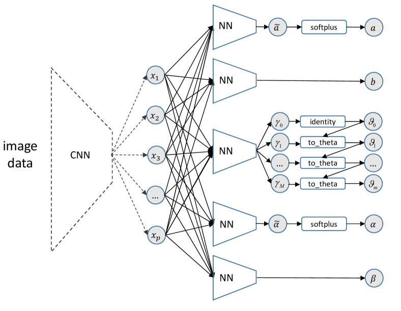
Figure 1: The network architecture of our model which is trained end-to-end starting with the input x yielding the conditional parameters of the transformation functions. The dashed CNN part is only used in case of image input data. If some parameters should be not depended on $x$, the respective NN gets a constant number (one) as input.

Our model has been implemented in R using Keras, TensorFlow, and TensorFlow Probability and can be found at: https://github.com/tensorchiefs/dl_mlt

Figure 2: Visual representation of the flow of Equation 6. The flow transforms from a bimodal distribution, such as the CPD in Figure 3 at $x=2.5$, to a standard Gaussian. For $f_{2}$ where the change from a bimodal to unimodal distributions happens the transformation function is also on display.

IV Experiments

In order to demonstrate the capacity of our proposed approach, we performed three different experiments.

IV-A One-Dimensional Toy Data

We use simulated toy data sets with a single feature and a single target variable to illustrate some properties of the proposed transformation model. In the first example the data generating process is given by imposing exponential noise with increasing amplitude on a linear increasing sinusoidal (see Figure 3). For some $x$-values two fitted CPDs are shown, one resulting from our NN based transformation model with $M=10$ (DL_MLT) Equation 8 and one from a less flexible linear transformation model (LTM) Equation 5. Figure 3 clearly demonstrates that the complex transformation model can, in contrast to the simple linear transformation model, cope with an non-monotone $x$-dependency of the variance. To quantify the goodness of fit, we us the negative log-likelihood (NLL) of the data (smaller is better), which is -2.00 for the complex and -0.85 for the simple linear transformation model.

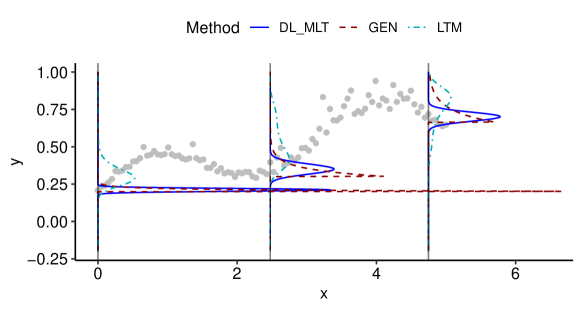
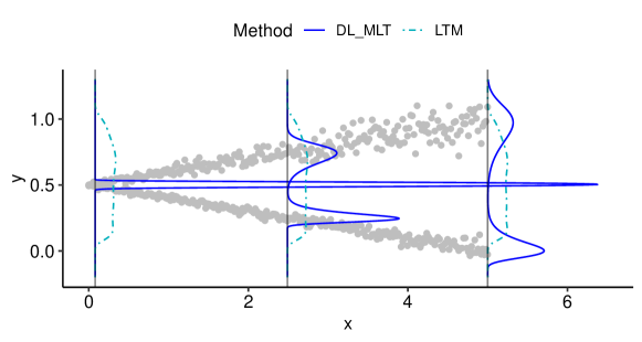
Figure 3: Simple one-dimensional toy example with complex outcome distributions. Training data is shown as gray points and the estimated CPDs for the linear transformation model (LTM) and the proposed DL_MLT method are shown for two data generating process as a dashed and solid lines, respectively. In the upper panel in addition the true CPD of the data generating process is shown (dotted line). The CPDs have been scaled down for plotting.

The second example, shown on the lower panel of Figure 3, is a challenging bimodal distribution in which the spread between the modes strongly depends on $x$ but the conditional mean of the outcome $y$ does not depend on $x$. Both models can capture the bimodal shape of the CPD, but the LTM is not flexible enough to adapt its bimodal CPD with changing $x$. The proposed flexible transformation model DL_MLT is able to also take the $x$ dependency of the spread between the modes of the distribution into account.

IV-B UCI-Benchmark Data Sets

TABLE I: Comparison of prediction performance (test NLL, smaller is better) on regression benchmark UCI datasets. The best method for each dataset is bolded, as are those with standard errors that overlap with the standard errors of the best method.

Data Set	N	DL_MLT	NGBoost	MC Dropout	Deep Ensembles	Gaussian Process	MDN	NFN
Boston	506	2.42 $\pm$ 0.050	2.43 $\pm$ 0.15	2.46 $\pm$0.25	2.41 $\pm$0.25	2.37 $\pm$0.24	2.49 $\pm$ 0.11	2.48 $\pm$0.11
Concrete	1030	3.29 $\pm$ 0.02	3.04 $\pm$ 0.17	3.04 $\pm$0.09	3.06 $\pm$0.18	3.03 $\pm$0.11	3.09 $\pm$ 0.08	3.03 $\pm$0.13
Energy	768	1.06 $\pm$ 0.09	0.60 $\pm$ 0.45	1.99 $\pm$0.09	1.38 $\pm$0.22	0.66 $\pm$0.17	1.04 $\pm$ 0.09	1.21 $\pm$0.08
Kin8nm	8192	-0.99 $\pm$ 0.01	-0.49 $\pm$ 0.02	-0.95 $\pm$0.03	-1.20 $\pm$0.02	-1.11 $\pm$0.03	NA	NA
Naval	11934	-6.54 $\pm$ 0.03	-5.34$\pm$ 0.04	-3.80 $\pm$0.05	-5.63 $\pm$0.05	-4.98 $\pm$0.02	NA	NA
Power	9568	2.85 $\pm$ 0.005	2.79 $\pm$ 0.11	2.80 $\pm$0.05	2.79 $\pm$0.04	2.81 $\pm$0.05	NA	NA
Protein	45730	2.63 $\pm$ 0.006	2.81 $\pm$ 0.03	2.89 $\pm$0.01	2.83 $\pm$0.02	2.89 $\pm$0.02	NA	NA
Wine	1588	0.67 $\pm$ 0.028	0.91 $\pm$ 0.06	0.93 $\pm$0.06	0.94 $\pm$0.12	0.95 $\pm$0.06	NA	NA
Yacht	308	0.004 $\pm$ 0.046	0.20 $\pm$ 0.26	1.55 $\pm$0.12	1.18 $\pm$0.21	0.10 $\pm$0.26	NA	NA

To compare the predictive performance of our NN based transformation model with other state-of-the-art methods, we use nine well established benchmark data sets (see table bench) from the UCI Machine Learning Repository. Shown is our approach (Deep_MLT), NGBoost [15], MC Dropout [4], Deep Ensembles [3], Gaussian Process [15], noise regularized Gaussian Mixture Density Networks (MDN) and normalizing flows networks (NFN) [10]. As hyperparameters for our Deep_MLT model, we used $M=10$ for all datasets and a $L_{2}$-regularization constants of 0.01 for the smaller datasets (Yacht, Energy, Concrete, and Boston) no regularization was used in the other datasets. To quantify the predictive performance, we use the negative log-likelihood (NLL) on test data. The NLL is a strictly proper score that takes its minimum if and only if the predicted CPD matches the true CPD and is therefore often used when comparing the performance of probabilistic models.

In order to compare with other state-of-art models, we follow the protocol from Hernandez and Lobato [16] that was also employed by Gal [4]. For validating our method, the benchmark data sets were split into several folds containing training data (90 percent) and test-data (10 percent). We downloaded the specific folds as used in [4] from https://github.com/yaringal/DropoutUncertaintyExps. We determined the hyperparameters of our model using 80 percent of the training data, keeping 20 percent for validation. The only preprocessing step has been a transformation to $[0,1]$ of $x$ and $y$ based on the training data. In contrast to other approaches in Table (I) like [4] and [15], we choose only one set of hyperparameters for each dataset and do not adapt the hyperparameters for each individual run separately. We can do this since our model has only few and quite stable hyperparameters. Specifically, we verified that the initial choice of the number of layers in the network is appropriate (no tuning has been done). We further choose the parameter of the $L_{2}$-regularization of the networks and the order $M$ of the Bernstein polynomials. After choosing the hyperparameters, we trained the same model again on the complete training fold and determined the NLL on the corresponding test fold. This procedure allowed us to compare the mean, the standard error of the test NLL with reported values from the literature.

The results in Table (I) show that our DL_MLT model yields, overall, a competitive performance with other state-of-the-art models. In the two tasks (Naval and Wine) the transformation model clearly outperforms all existing models. We followed up on the reasons and visually inspected the predicted CPDs in the different tasks. For Naval, we found that the model needs extremely long training periods, approximately 120’000 iterations compared to approximately 20’000, for the other data sets. When trained for such as a period it’s CPD is a very narrow single spike (see lower left panel in Figure 4). We speculate that the reason for worse NLL of the other models is that they have not been trained long enough. For the other data-sets, were we outperformed the existing methods, the striking finding was, that for many instances very non-Gaussian CPDs are predicted. For the Wine dataset the predicted CPDs are not always uni-model but quite often show a multi-modal shape (see upper right panel in Figure 4). This makes perfectl sense, since the target variable in the dataset, the subjective quality of the wine is an integer value ranging from 0 to 10. Hence, if the model cannot decide between two levels, it predicts a bimodal CPD , which shows that it can learn to a certain extend the discrete structure of the data (see upper right panel in Figure 4).

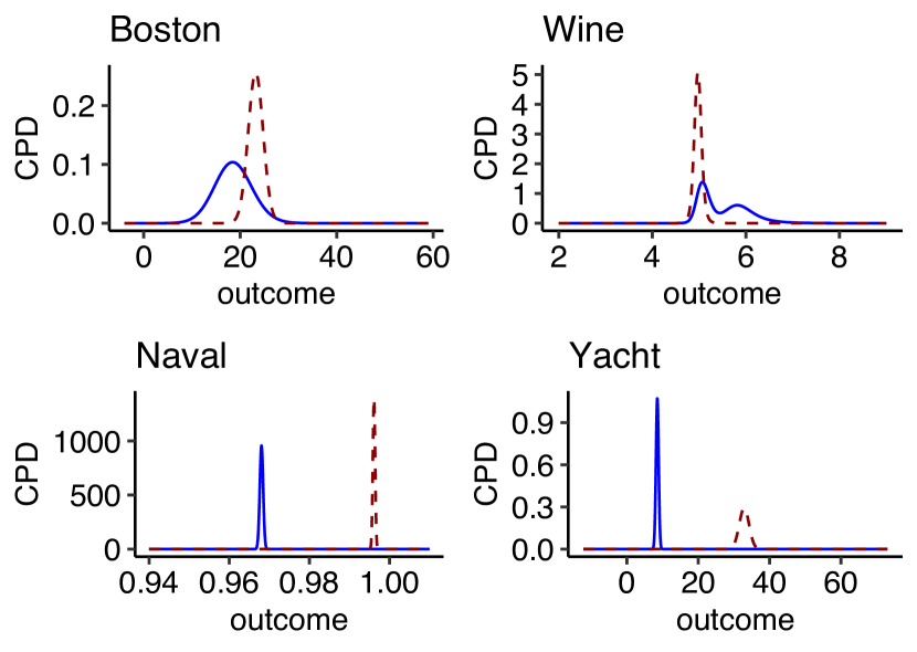
Figure 4: Predicted CPDs for test data in the benchmark data Boston, Wine, Naval, and Yacht are shown. For each data set two test observations with commonly observed CPD shapes were picked (depicted with solid and dashed lines respectively).

To investigate if we need more flexibility to model this kind of multi-modal outcome distributions, we refitted the Wine data with $M=20$ and obtained an significantly improved test NLL of $0.40\pm 0.025$. For the other data-sets the underlying cause of the better performance of our DL_MLT model is unclear to us.

IV-C Age Estimation from Faces

In this experiment, we want to demonstrate the usefulness of the proposed NN based transformation model for a typical deep learning context dealing with complex input data, like images. For this purpose, we choose the UTKFace dataset containing $N=23’708$ images of cropped faces of humans with known age ranging from 1 to 116 years [17]. The spread of the CPD indicates the uncertainty of the model about the age. We did not do any hyperparameter search for this proof of concept and used 80 percent of the data for training. The color images of size $(200,200,3)$ were downscaled to $(64,64,3)$ and feed into a small convolutional neural network (CNN) comprising three convolutional layers with 141840 parameters, as indicated in Figure 1.

Estimating the age is a challenging problem. First, age is non negative. Second, depending on the age, it is more or less hard to estimate the age. As humans we would probably be not more than two years off when estimating the age of a one year old infant, but for a thirty or ninety year old person the task is much harder. Therefore, we expect that also a probabilistic model will predict CPDs with different spreads and shapes. Usually this problem is circumvented by transforming the age by e.g. a log transformation. Here, we did not apply any transformation to the raw data and let the network find to correct CPD in an end-to-end fashion. After training for 15’000 iterations, a NLL of 3.83 on the test-set has been reached. Since we did not find a suitable probabilistic benchmark for the dataset, we show in Figure 5 some typical results for the CPD for people of different ages.

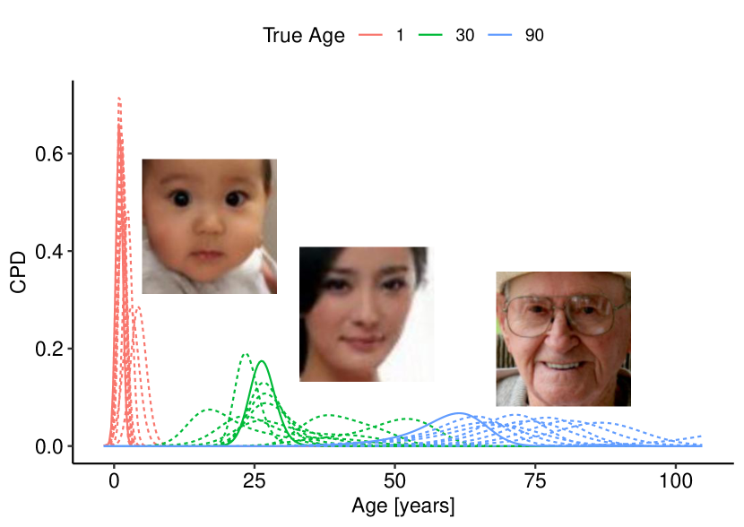
Figure 5: CPD for different ages. Shown are 10 randomly picked results of the test set for different true ages (1, 30, and 90 years), the shown images correspond to the solid lines.

The results of the model meet our expectations yielding narrow CPDs for infants, while for older people the spread of the CPD broadens with increasing age.

V Conclusion and outlook

We have demonstrated that deep transformation models are a powerful approach for probabilistic regression tasks, where for each input $x$ a conditional probability distribution on $y$ is predicted. Such probabilistic models are needed in many real-world situations where the available information does not deterministically define the outcome and where an estimate of the uncertainty is needed.

By joining ideas from statistical transformation models and deep normalizing flows the proposed model is able to outperform existing models from both fields when the shape of the conditional distribution is complex and far away from a Gaussian.

Compared to statistical transformation models the proposed deep transformation model does not require predefined features. It can be trained in an end-to-end fashion from complex data like images by prepending a CNN.

Though mixture density networks [2] are able to handle non-Gaussian CPDs they often tend to overfit the data and require a careful tuning of regularization to reach a good performance [10]. Since deep transformation models estimate a smooth, monotonically increasing transformation function, they always yield smooth conditional distributions. Therefore, we need only mild regularization in cases where the NN for the parameter estimation would overfit the train data. For the UCI-datasets, we empirically observed the need for mild regularization only in cases the size of the dataset is below 1500 points.

The proposed model can, in principle, be extended to higher dimensional cases of the response variable $y$, see [13] for a statistical treatment. The fact that our model is very flexible and does not impose any restriction on the modeled CPD, allows it to learn the restrictions of the dataset, like age being positive, from the data. For limited training data that can lead to situations where some probability is also assigned to impossible outcomes, such as negative ages. It is possible to adapt our model to respect these kind of limitations or to predict e.g. discrete CPDs. We will tackle this in future research. For discrete data we will use the appropriate likelihood that is described in terms of the corresponding discrete density $\Phi(h(y\mid x))-\Phi(h(y-\mid x))$, where $y$ is the observed value and $y-$ the largest value of the discrete support with $y-<y$. For the Wine dataset for example, where the outcome is an ordered set of ten answer categories, such an approach would result in a discrete predictive model matching the outcome $y$. At the moment, we also did not incorporate the ability to handle truncated or censored data which is possible with statistical transformation models, see [12]. For the Boston dataset for example, all values with $y=50$ are in fact right-censored, thus the probability $1-\Phi(h(50\mid x))$ would be the correct contribution to the likelihood.

Another limitation of the proposed flexible transformation NN is its black box character. Picking special base distributions, such as the standard logistic or minimum extreme value distributions, and using linear transformation models should allow to disentangle and describe the effect of different input features by means of mean shifts, odds ratios, or hazard ratios. This can be translated into interpretable deep learning transformation models, which we plan to do in the near future.

References

- [1] Y. Lecun, Y. Bengio, and G. Hinton, “Deep learning,” pp. 436–444, may 2015.
- [2] C. M. Bishop, “Mixture Density Networks,” Tech. Rep., 1994. [Online]. Available: http://www.ncrg.aston.ac.uk/
- [3] B. Lakshminarayanan, A. Pritzel, and C. Blundell, “Simple and Scalable Predictive Uncertainty Estimation using Deep Ensembles,” in Advances in Neural Information Processing Systems 30, I. Guyon, U. V. Luxburg, S. Bengio, H. Wallach, R. Fergus, S. Vishwanathan, and R. Garnett, Eds. Curran Associates, Inc., 2017, pp. 6402–6413.
- [4] Y. Gal and Z. Ghahramani, “Dropout as a Bayesian Approximation: Representing Model Uncertainty in Deep Learning,” 33rd International Conference on Machine Learning, ICML 2016, vol. 3, pp. 1651–1660, jun 2015. [Online]. Available: http://arxiv.org/abs/1506.02142
- [5] Y. Gal, J. Hron, and A. Kendall, “Concrete Dropout,” Advances in Neural Information Processing Systems, vol. 2017-December, pp. 3582–3591, may 2017. [Online]. Available: http://arxiv.org/abs/1705.07832
- [6] D. J. Rezende and S. Mohamed, “Variational Inference with Normalizing Flows,” 32nd International Conference on Machine Learning, ICML 2015, vol. 2, pp. 1530–1538, may 2015. [Online]. Available: http://arxiv.org/abs/1505.05770
- [7] G. Papamakarios, E. Nalisnick, D. J. Rezende, S. Mohamed, and B. Lakshminarayanan, “Normalizing Flows for Probabilistic Modeling and Inference,” dec 2019. [Online]. Available: http://arxiv.org/abs/1912.02762
- [8] D. P. Kingma and P. Dhariwal, “Glow: Generative Flow with Invertible 1x1 Convolutions,” Advances in Neural Information Processing Systems, vol. 2018-Decem, pp. 10 215–10 224, jul 2018. [Online]. Available: http://arxiv.org/abs/1807.03039
- [9] B. L. Trippe and R. E. Turner, “Conditional density estimation with bayesian normalising flows,” arXiv preprint arXiv:1802.04908, 2018.
- [10] J. Rothfuss, F. Ferreira, S. Boehm, S. W. arXiv preprint arXiv …, and U. 2019, “Noise Regularization for Conditional Density Estimation,” arxiv.org, 2019. [Online]. Available: https://arxiv.org/abs/1907.08982
- [11] G. E. P. Box and D. R. Cox, “An Analysis of Transformations,” Journal of the Royal Statistical Society: Series B (Methodological), vol. 26, no. 2, pp. 211–243, jul 1964.
- [12] T. Hothorn, L. Möst, and P. Bühlmann, “Most Likely Transformations,” Scandinavian Journal of Statistics, vol. 45, no. 1, pp. 110–134, mar 2018. [Online]. Available: http://doi.wiley.com/10.1111/sjos.12291
- [13] N. Klein, T. Hothorn, and T. Kneib, “Multivariate conditional transformation models,” arXiv preprint arXiv:1906.03151, 2019.
- [14] Y. Tian, T. Hothorn, C. Li, F. E. Harrell Jr., and B. E. Shepherd, “An empirical comparison of two novel transformation models,” Statistics in Medicine, vol. 39, no. 5, pp. 562–576, 2020.
- [15] T. Duan, A. Avati, D. Y. Ding, K. K. Thai, S. Basu, A. Y. Ng, and A. Schuler, “NGBoost: Natural Gradient Boosting for Probabilistic Prediction,” oct 2020. [Online]. Available: http://arxiv.org/abs/1910.03225
- [16] J. M. Hernández-Lobato and R. Adams, “Probabilistic backpropagation for scalable learning of bayesian neural networks,” in International Conference on Machine Learning, 2015, pp. 1861–1869.
- [17] Z. Zhang, Y. Song, and H. Qi, “Age Progression/Regression by Conditional Adversarial Autoencoder,” Tech. Rep. [Online]. Available: https://zzutk.github.io/Face-Aging-CAAE