A locking-free DPG scheme for Timoshenko beams

Abstract

We develop a discontinuous Petrov–Galerkin scheme with optimal test functions (DPG method) for the Timoshenko beam bending model with various boundary conditions, combining clamped, supported, and free ends. Our scheme approximates the transverse deflection and bending moment. It converges quasi-optimally in $L_{2}$ and is locking free. In particular, it behaves well (converges quasi-optimally) in the limit case of the Euler–Bernoulli model. Several numerical results illustrate the performance of our method.

Key words: beam bending, Timoshenko model, Euler–Bernoulli model, discontinuous Petrov–Galerkin method, optimal test functions.

AMS Subject Classifications: 74S05, 74K10, 65L11, 65L60

1 Introduction

Thin structures like beams, plates, and shells form an important area of research in solid mechanics. The Reissner–Mindlin model is among the most widely used for the analysis of plate bending. The corresponding one-dimensional case is the Timoshenko model for beam bending. Numerical schemes for these models are tricky to design due to the presence of the thickness parameter, $t$, which induces a singular perturbation when $t\to 0$ in the case of plates. Not carefully designed approximation schemes suffer from locking. Mathematically, the limit cases (setting $t=0$ in the scaled models) correspond to the Kirchhoff–Love and Euler–Bernoulli models in the case of plates and beams, respectively.

There is extensive literature on the numerical analysis of these models generally, though with fewer results from the mathematics community on the Kirchhoff–Love model, which can suffer from a lack of regularity. We do not discuss the many contributions that exist but mention some mathematically focused paper, on the discontinuous Galerkin scheme for Euler–Bernoulli beams from Baccouch [1], and on locking-free $hp$ finite element approaches for Timoshenko beams from Li and Celiker et al. [14, 3]. More recently, Lepe et al. presented a locking-free mixed finite element scheme for the Timoshenko model [13].

Here we continue our study of discontinuous Petrov–Galerkin schemes with optimal test functions (DPG method) for singularly perturbed problems. The underlying idea consists in using product (“broken”) test spaces and optimal test functions to automatically satisfy discrete inf–sup properties of Galerkin schemes for any well-posed variational formulation, see the early works of Demkowicz and Gopalakrishnan, e.g., [6]. In order to obtain robust (or locking-free) approximations it is critical to select appropriate test norms [7, 4], possibly in combination with specifically designed variational formulations [12, 11], or adaptively improved test functions [5].

In this paper we develop a locking-free DPG method for Timoshenko beams that also works in the limit case of thickness zero (in a scaled version), the Euler–Bernoulli model. We use our knowledge of variational formulations for fourth-order problems that we have obtained from our work on the Kirchhoff–Love plate bending model [10, 9, 8], and on the Reissner–Mindlin plate model [11]. Specifically, we follow [11] where we developed an ultraweak formulation based on the deflection and bending moment, and included the gradient of the deflection as an independent unknown. The Reissner–Mindlin model has some critical regularity issues, with weaker deflection and stronger bending moment compared to the Kirchhoff–Love situation. This makes the analysis interesting. The techniques presented in this paper for the Timoshenko beam model are based on those from [11]. But, instead of closely following the same paths, we simplify procedures and shorten proofs since in the one-dimensional situation regularity properties are much simpler. For instance, considering $L_{2}$ regular distributed forces, both the deflection and bending moment variables are $H^{2}$-regular. Therefore, we can avoid using the additional gradient variable without complicating the theoretical analysis. Furthermore, the sophisticated trace operators from [11] dramatically simplify. Due to the $H^{2}$-regularities we are able to use some techniques from [8] where we studied the bi-Laplacian in higher space dimensions.

Finally we note that Niemi et al. [15] have used DPG techniques for beams before. Though they only consider a cantilever with tip load, without distributed load or different boundary conditions, and assume the beam thickness to be fixed.

The remainder of this paper is organized as follows. In Section 2 we present the model problem, develop an ultraweak variational formulation, and state its well-posedness (Theorem 1). The DPG scheme is briefly presented in Section 3, and Theorem 2 states its robust quasi-optimal convergence. Section 4 gives a proof of the well-posedness of our variational formulation, split into several lemmas. Various numerical experiments for different thickness parameters and boundary conditions are presented in Section 5. They confirm that our scheme is locking free.

Throughout this paper, $a\lesssim b$ means that $a\leq cb$ with a generic constant $c>0$ that is independent of the thickness parameter $t$ and the underlying mesh. Similarly, we use the notation $a\gtrsim b$ and $a\simeq b$.

2 Model problem and variational formulation

We consider the scaled dimensionless stationary Timoshenko model for beam bending, formulated as in [15] (though with different sign for the bending moment):

$$t^{2}Q=\theta(u^{\prime}-\psi),\quad-M=\psi^{\prime},\quad-Q^{\prime}=p,\quad M^{\prime}-kQ=0\qquad\text{in}\quad\ I:=(0,1).$$

Here, $u$, $\psi$, $Q$, $M$ are, respectively, the transverse deflection, the rotation of the beam’s cross section, the shear force, and the bending moment. The beam has length $1$ and thickness $t$. We assume that $t\in[0,1]$. Furthermore, $p$ is the distributed force and $k$, $\theta$ are constants. As in [10, 11] for plate problems, we develop a scheme that approximates the deflection and bending moment variables. To this end we replace $Q$ by using the relation $M^{\prime}-kQ=0$ and eliminate $\psi$, obtaining

$$-M^{\prime\prime}=f:=kp,\qquad t^{2}M^{\prime\prime}=k\theta(u^{\prime\prime}+M).$$

For simplicity we set $k\theta=1$. This parameter is not critical. The strong form of our model problem then is

$$-M^{\prime\prime}=f,\quad M-t^{2}M^{\prime\prime}+u^{\prime\prime}=0\qquad\text{in}\quad I.$$ (1)

We note that as expected, setting $t=0$, the Timoshenko model reduces to the Euler–Bernoulli model. In the following we assume that $f\in L_{2}(I)$. Then, $u,M\in H^{2}(I)$.

It remains to specify boundary conditions. We consider all the physically relevant combinations of clamped end (deflection and rotation are given), supported end (deflection and bending moment are given), and free end (bending moment and shear force are given), for simplicity of presentation with homogeneous data only. We note that it is straightforward to consider non-homogeneous boundary data since all the relevant traces are present in our formulation. Using the relation $\psi=u^{\prime}-t^{2}M^{\prime}$ for the rotation, the boundary conditions are

$$\begin{array}[]{llllllllll}\text{clamped-clamped:}&u(0)=0,&u^{\prime}(0)=t^{2}M^{\prime}(0),&u(1)=0,&u^{\prime}(1)=t^{2}M^{\prime}(1),\\ \text{clamped-supported:}&u(0)=0,&u^{\prime}(0)=t^{2}M^{\prime}(0),&u(1)=0,&M(1)=0,\\ \text{clamped-free:}&u(0)=0,&u^{\prime}(0)=t^{2}M^{\prime}(0),&M(1)=0,&M^{\prime}(1)=0,\\ \text{supported-supported:}&u(0)=0,&M(0)=0,&u(1)=0,&M(1)=0.\end{array}$$ (2)

The corresponding solution spaces are

$$\mathbb{H}^{2}_{cc}(t):=\{(u,M)\in H^{2}(I)\times H^{2}(I);\;u(0)=u^{\prime}(0)-t^{2}M^{\prime}(0)=u(1)=u^{\prime}(1)-t^{2}M^{\prime}(1)=0\},$$

$$\mathbb{H}^{2}_{cs}(t):=\{(u,M)\in H^{2}(I)\times H^{2}(I);\;u(0)=u^{\prime}(0)-t^{2}M^{\prime}(0)=u(1)=M(1)=0\},$$

$$\mathbb{H}^{2}_{cf}(t):=\{(u,M)\in H^{2}(I)\times H^{2}(I);\;u(0)=u^{\prime}(0)-t^{2}M^{\prime}(0)=M(1)=M^{\prime}(1)=0\},$$

$$\mathbb{H}^{2}_{ss}(t):=\{(u,M)\in H^{2}(I)\times H^{2}(I);\;u(0)=M(0)=u(1)=M(1)=0\}.$$

Of course, $\mathbb{H}^{2}_{ss}(t)$ is independent of $t$.

Now we derive an ultraweak formulation of our Timoshenko beam problem. For a positive integer $n$ and nodes $0=x_{0}<x_{1}<x_{2}<\ldots<x_{n}=1$, let us consider the partition $\mathcal{T}=\{I_{j}=(x_{j-1},x_{j});\;j=1,\ldots,n\}$ of $I$. Below, we denote $h_{j}:=x_{j}-x_{j-1}$ ($j=1,\ldots,n$). Testing the equations from (1) respectively with

$$z,W\in H^{2}(\mathcal{T}):=\{v\in L_{2}(I);\;v_{j}:=v|_{I_{j}}\in H^{2}(I_{j}),\ j=1,\ldots,n\},$$

integration by parts gives

$$(u\hskip 1.42262pt,W^{\prime\prime})_{\mathcal{T}}+(M\hskip 1.42262pt,W+z^{\prime\prime}-t^{2}W^{\prime\prime})_{\mathcal{T}}$$

$$+\sum_{j=1}^{n}\Bigl{(}-\bigl{[}u\,W^{\prime}\bigr{]}_{j}+\bigl{[}M^{\prime}\,z\bigr{]}_{j}-\bigl{[}M\,(z^{\prime}-t^{2}W^{\prime})\bigr{]}_{j}+\bigl{[}(u^{\prime}-t^{2}M^{\prime})\,W\bigr{]}_{j}\Bigr{)}=-(f\hskip 1.42262pt,z).$$ (3)

Here, $(\cdot\hskip 1.42262pt,\cdot)$ denotes the $L_{2}(I)$-inner product with norm $\|\cdot\|$, and $(\cdot\hskip 1.42262pt,\cdot)_{\mathcal{T}}$ indicates the $L_{2}$-inner product that is taken piecewise on $\mathcal{T}$. The $L_{2}(T)$-norm ($T\in\mathcal{T}$) will be denoted by $\|\cdot\|_{T}$. Furthermore, $[\,\cdot\,]_{j}$ are the boundary terms from the integration-by-parts formula on $I_{j}$. That is, e.g., $[u\,W^{\prime}]_{j}=u(x_{j})W^{\prime}(x_{j})-u(x_{j-1})W^{\prime}(x_{j-1})$ where the point evaluations are taken from $u$ and $W$ restricted to $I_{j}$ ($j=1,\ldots,n$).

Introducing the following maps for the point evaluations,

$$H^{2}(I_{j})\ni z\mapsto \gamma_{j}(z):=(z(x_{j-1}),z^{\prime}(x_{j-1}),z(x_{j}),z^{\prime}(x_{j})),\quad j=1,\ldots,n,$$

$$H^{2}(\mathcal{T})\ni z\mapsto \gamma_{h}(z):=\Bigl{(}\gamma_{j}(z_{j}))\Bigr{)}_{j=1}^{n}$$

(note that $z_{j}=z|_{I_{j}}$), the point evaluations from (2) are abbreviated as

$$\langle{}\gamma_{h}(u,M),(z,W)\rangle_{t}:=\sum_{j=1}^{n}\Bigl{(}-\bigl{[}u\,W^{\prime}\bigr{]}_{j}+\bigl{[}M^{\prime}\,z\bigr{]}_{j}-\bigl{[}M\,(z^{\prime}-t^{2}W^{\prime})\bigr{]}_{j}+\bigl{[}(u^{\prime}-t^{2}M^{\prime})\,W\bigr{]}_{j}\Bigr{)}.$$

Here we abuse the notation and write $\gamma_{h}(u,M)=(\gamma_{h}(u),\gamma_{h}(M))$. Of course, for $u\in H^{2}(I)$, $\gamma_{h}(u)$ gives rise to $2n+2$ independent real numbers ($\gamma_{h}$ induces a continuous surjective mapping from $H^{2}(I)$ to $\mathbb{R}^{2n+2}$), and we note that

$$\langle{}\gamma_{h}(u,M),(z,W)\rangle_{t}=-\langle{}\gamma_{h}(z,W),(u,M)\rangle_{t}\quad\forall u,M,z,W\in H^{2}(\mathcal{T}).$$

For all of the boundary conditions from (2), $\gamma_{h}(u,M)$ allows for $4n$ independent scalar unknowns. Specifically, depending on the type of boundary condition, we denote

$${\hat{U}}_{a}(t):=\gamma_{h}(\mathbb{H}^{2}_{a}(t)),\quad a\in\{cc,cs,cf,ss\}.$$

As noted before, the dimension of any of these spaces is $4n$, and ${\hat{U}}_{ss}(t)$ is independent of $t$. We also need the image

$${\hat{U}}:=\gamma_{h}(H^{2}(I)\times H^{2}(I))=(\gamma_{h}(H^{2}(I)),\gamma_{h}(H^{2}(I))=\mathbb{R}^{4n+4}.$$

A duality between any of these spaces with $H^{2}(\mathcal{T})\times H^{2}(\mathcal{T})$ is also denoted by $\langle{}\cdot,\cdot\rangle_{t}$, defined as

$$\langle{}{\hat{q}},(z,W)\rangle_{t}:=\langle{}\gamma_{h}(u,M),(z,W)\rangle_{t}\quad\text{for}\quad u,M\in H^{2}(I)\ \text{with}\ \gamma_{h}(u,M)={\hat{q}}.$$

Now, to present the ultraweak variational formulation of (1) with one of the boundary conditions (2), we denote the solution space as

$$U_{a}(t):=L_{2}(I)\times L_{2}(I)\times{\hat{U}}_{a}(t)\quad\text{with}\quad a\in\{cc,cs,cf,ss\}\quad\text{as needed},$$

and the test space as

$$V:=H^{2}(\mathcal{T})\times H^{2}(\mathcal{T}).$$

Defining the norms (squared)

$$\|\gamma_{j}(u)\|_{j}^{2} :=\frac{h_{j}}{420}\Bigl{[}156\bigl{(}u(x_{j-1})^{2}+u(x_{j})^{2}\bigr{)}+4h_{j}^{2}\bigl{(}u^{\prime}(x_{j-1})^{2}+u^{\prime}(x_{j})^{2}\bigr{)}$$

$$\qquad+108u(x_{j-1})u(x_{j})+44h_{j}\bigl{(}u(x_{j-1})u^{\prime}(x_{j-1})-u(x_{j})u^{\prime}(x_{j})\bigr{)}$$

$$\qquad-6h_{j}^{2}u^{\prime}(x_{j-1})u^{\prime}(x_{j})+26h_{j}\bigl{(}u(x_{j})u^{\prime}(x_{j-1})-u(x_{j-1})u^{\prime}(x_{j})\bigr{)}\Bigr{]}$$

$$+\frac{2}{h_{j}^{3}}\Bigl{[}6\bigl{(}u(x_{j-1})^{2}-2u(x_{j-1})u(x_{j})+u(x_{j})^{2}\bigr{)}+2h_{j}^{2}\bigl{(}u^{\prime}(x_{j-1})^{2}+u^{\prime}(x_{j-1})u^{\prime}(x_{j})+u^{\prime}(x_{j})^{2}\bigr{)}$$

$$\qquad+6h_{j}\bigl{(}u(x_{j-1})u^{\prime}(x_{j-1})-u(x_{j})u^{\prime}(x_{j})+u(x_{j-1})u^{\prime}(x_{j})-u(x_{j})u^{\prime}(x_{j-1})\bigr{)}\Bigr{]},$$ (4)

$$\|\gamma_{h}(u,M)\|_{h}^{2}:=\sum_{j=1}^{n}\Bigl{(}\|\gamma_{j}(u_{j})\|_{j}^{2}+\|\gamma_{j}(M_{j})\|_{j}^{2}\Bigr{)} (u,M\in H^{2}(I)),$$

$$\|z\|_{2,T}^{2}:=\|z\|_{T}^{2}+\|z^{\prime\prime}\|_{T}^{2} (z\in H^{2}(T),\ T\in\mathcal{T}),$$

$$\|z\|_{2}^{2}:=\|z\|^{2}+\|z^{\prime\prime}\|^{2} (z\in H^{2}(I)),$$

$$\|z\|_{2,\mathcal{T}}^{2}:=\|z\|^{2}+(z^{\prime\prime}\hskip 1.42262pt,z^{\prime\prime})_{\mathcal{T}} (z\in H^{2}(\mathcal{T})),$$

these spaces are normed as follows,

$$\|(u,M,{\hat{q}})\|_{U}^{2}:=\|u\|^{2}+\|M\|^{2}+\|{\hat{q}}\|_{h}^{2}\quad\text{and}\quad\|(z,W)\|_{V}^{2}:=\|z\|_{2,\mathcal{T}}^{2}+\|W\|_{2,\mathcal{T}}^{2}$$

for $(u,M,{\hat{q}})\in U_{a}(t)$ ($a\in\{cc,cs,cf,ss\}$) and $z,W\in H^{2}(\mathcal{T})$. Finally, defining the functional $L_{f}(z,W):=-(f\hskip 1.42262pt,z)$ and bilinear form

$$b_{t}((u,M,{\hat{q}}),(z,W)):=(u\hskip 1.42262pt,W^{\prime\prime})_{\mathcal{T}}+(M\hskip 1.42262pt,W+z^{\prime\prime}-t^{2}W^{\prime\prime})_{\mathcal{T}}+\langle{}{\hat{q}},(z,W)\rangle_{t},$$

the variational formulation is:

$$(u,M,{\hat{q}})\in U_{a}(t):\quad b_{t}((u,M,{\hat{q}}),(z,W))=L_{f}(z,W)\quad\forall(z,W)\in V.$$ (5)

Our first main result is the well-posedness of (5).

Theorem 1.

Given $f\in L_{2}(I)$, $a\in\{cc,cs,cf,ss\}$, and $t\in[0,1]$, there exists a unique solution $(u,M,{\hat{q}})\in U_{a}(t)$ of (5). It satisfies

$$\|(u,M,{\hat{q}})\|_{U(t)}\lesssim\|f\|$$

with a hidden constant that is independent of $\mathcal{T}$, $f$, and $t$. Furthermore, $(u,M)$ solves (1), and ${\hat{q}}=\gamma_{h}(u,M)$.

3 The DPG method

Our DPG method is a Petrov–Galerkin scheme based on formulation (5). We consider a finite-dimensional subspace $U_{a,h}(t)\subset U_{a}(t)$ and select test functions $(z,W)\in{\rm T}_{t}(U_{a,h}(t))$ where ${\rm T}_{t}$ is the trial-to-test operator ${\rm T}_{t}:\;U_{a}(t)\to V$ defined by

$$\llangle{\rm T}_{t}(u,M,{\hat{q}})\hskip 1.42262pt,(z,W)\rrangle_{V}=b_{t}((u,M,{\hat{q}}),(z,W))\quad\forall(z,W)\in V.$$

Here, $\llangle\cdot\hskip 1.42262pt,\cdot\rrangle_{V}$ is the inner product in $V$,

$$\llangle(z,W)\hskip 1.42262pt,({\delta\!z},{\delta\!W})\rrangle_{V}=(z\hskip 1.42262pt,{\delta\!z})+(z^{\prime\prime}\hskip 1.42262pt,{\delta\!z}^{\prime\prime})+(W\hskip 1.42262pt,{\delta\!W})+(W^{\prime\prime}\hskip 1.42262pt,{\delta\!W}^{\prime\prime}).$$

Our DPG approximation $(u_{h},M_{h},{\hat{q}}_{h})\in U_{a,h}(t)$ is defined by

$$b_{t}((u_{h},M_{h},{\hat{q}}_{h}),{\rm T}_{t}({\delta\!u},{\delta\!M},{\delta\!{\hat{q}}}))=L({\rm T}_{t}({\delta\!u},{\delta\!M},{\delta\!{\hat{q}}}))\quad\forall({\delta\!u},{\delta\!M},{\delta\!{\hat{q}}})\in U_{a,h}(t).$$ (6)

Since the DPG-approximation minimizes the residual in the $V$-norm, cf. [6], and since the $U$-norm is uniformly equivalent to the dual norm of $V$, cf. (14) below, our approximation is quasi-optimal in the $U$-norm. Let us formulate this result.

Theorem 2.

Let $a\in\{cc,cs,cf,ss\}$, $f\in L_{2}(I)$ and $t\in[0,1]$ be given. There exists a unique solution $(u_{h},M_{h},{\hat{q}}_{h})\in U_{a,h}(t)$ to (6). It satisfies

$$\|u-u_{h}\|+\|M-M_{h}\|+\|{\hat{q}}-{\hat{q}}_{h}\|_{h}\lesssim\inf\{\|u-v_{h}\|+\|M-Q_{h}\|;\;(v_{h},Q_{h})\in U_{a,h}(t)\}$$

with a hidden constant that is independent of $f,\mathcal{T},U_{a,h}(t)$, and $t$.

4 Proof of Theorem 1

We split the proof of Theorem 1 into several parts. This is standard procedure, cf., e.g., [2, 8, 11]. Specifically, we closely follow the presentation from [11]. The steps consist in, (a) characterizing the norms for the trace space ${\hat{U}}$ which is finite-dimensional (Lemma 3), (b) checking that test functions become continuous when annihilated by trace elements (Lemma 4), (c) proving stability of the adjoint problem (Lemma 5), and (d) checking injectivity of the operator that is adjoint to problem (1) (Lemma 6).

Lemma 3.

$$\sup_{(z,W)\in V\setminus\{0\}}\frac{\langle{}{\hat{q}},(z,W)\rangle_{t}}{\|(z,W)\|_{V}}\simeq\|{\hat{q}}\|_{h,t}\quad\forall{\hat{q}}\in{\hat{U}},\ t\in[0,1].$$

Proof.

Step 1. We start by making three observations. First,

$$(z,W)\mapsto(\tilde{z},\widetilde{W}):=(z+t^{2}W,W)$$ (7)

is an automorphism in $V=H^{2}(\mathcal{T})\times H^{2}(\mathcal{T})$ that is uniformly bounded with respect to $t$ in both directions. Second,

$$\langle{}\gamma_{h}(u,M),(\tilde{z},\widetilde{W})\rangle_{t} =\sum_{j=1}^{n}\Bigl{(}-\bigl{[}u\,W^{\prime}\bigr{]}_{j}+\bigl{[}M^{\prime}\,z\bigr{]}_{j}-\bigl{[}M\,z^{\prime}\bigr{]}_{j}+\bigl{[}u^{\prime}\,W\bigr{]}_{j}\Bigr{)}$$

$$=-(u\hskip 1.42262pt,W^{\prime\prime})_{\mathcal{T}}+(u^{\prime\prime}\hskip 1.42262pt,W)-(M\hskip 1.42262pt,z^{\prime\prime})_{\mathcal{T}}+(M^{\prime\prime}\hskip 1.42262pt,z)$$ (8)

holds for $u,M\in H^{2}(I)$ and $z,W\in H^{2}(\mathcal{T})$, and third, as in [8, Lemma 1] for the Laplacian, one proves that

$$\sup_{{\delta\!v}\in H^{2}(T)\setminus\{0\}}\frac{(v\hskip 1.42262pt,{\delta\!v}^{\prime\prime})_{T}-(v^{\prime\prime}\hskip 1.42262pt,{\delta\!v})_{T}}{\|{\delta\!v}\|_{2,T}}\\ =\inf\{\|w\|_{2,T};w\in H^{2}(T),\ w(x_{i})=v(x_{i}),\ w^{\prime}(x_{i})=v^{\prime}(x_{i}),\ i=j-1,j\}\quad(T=I_{j}\in\mathcal{T})$$

holds for any $v\in H^{2}(T)$. Therefore, one deduces that

$$\sup_{(z,W)\in V\setminus\{0\}}\frac{\langle{}{\hat{q}},(z,W)\rangle_{t}}{\|(z,W)\|_{V}}\simeq\\ \inf\{\|v\|_{2};\;v\in H^{2}(I),\ \gamma_{h}(v)={\hat{q}}_{1}\}+\inf\{\|v\|_{2};\;v\in H^{2}(I),\ \gamma_{h}(v)={\hat{q}}_{2}\}$$

holds where ${\hat{q}}=({\hat{q}}_{1},{\hat{q}}_{2})$. Noting that the norms on the right-hand side localize (the minima can be calculated element-wise), it remains to show the local relation

$$\inf\{\|v\|_{2,T};\;v\in H^{2}(T),\ \gamma_{j}(v)=\gamma_{j}(u)\}\simeq\|\gamma_{j}(u)\|_{j}\quad\forall u\in H^{2}(T),\ T=I_{j},\ j=1,\ldots,n.$$ (9)

Step 2. To prove (9) it is enough to consider an element $I_{h}=(0,h)$ of length $h\in(0,1]$. Let $u\in H^{2}(I_{h})$ be given and set ${\hat{q}}_{u}=\gamma(u):=(u(0),u^{\prime}(0),u(h),u^{\prime}(h))$. It follows that

$$\inf\{\|v\|_{2,I_{h}};\;v\in H^{2}(T),\ \gamma(v)={\hat{q}}_{u}\}=\|w_{u}\|_{2,I_{h}}$$

where $w_{u}\in H^{2}(I_{h})$ solves

$$w_{u}^{(4)}+w_{u}=0\quad\text{in}\ I_{h},\quad\gamma(w_{u})={\hat{q}}_{u}.$$

We also define $v_{u}\in H^{2}(I_{h})$ as the solution to

$$v_{u}^{(4)}=0\quad\text{in}\ I_{h},\quad\gamma(v_{u})={\hat{q}}_{u}.$$ (10)

It follows that $\|w_{u}\|_{2,I_{h}}\leq\|v_{u}\|_{2,I_{h}}$ (since $w_{u}$ minimizes the $H^{2}(I_{h})$-norm) and $|v_{u}|_{2,I_{h}}:=\|v_{u}^{\prime\prime}\|_{I_{h}}\leq|w_{u}|_{2,I_{h}}\leq\|w_{u}\|_{2,I_{h}}$ (since $v_{u}$ minimizes the $H^{2}(I_{h})$-seminorm). Proving that $\|v_{u}\|_{I_{h}}\lesssim\|w_{u}\|_{2,I_{h}}$ then gives the uniform equivalence $\|v_{u}\|_{2,I_{h}}\simeq\|w_{u}\|_{2,I_{h}}$. To show this, let $z\in H^{2}(I_{h})$ solve

$$z^{(4)}=v_{u}\quad\text{in}\ I_{h},\quad\gamma(z)=0.$$

Then, integrating by parts, using that $\gamma(w_{u})=\gamma(v_{u})$ and $(v_{u}^{\prime\prime}\hskip 1.42262pt,z^{\prime\prime})_{I_{h}}=0$ by (10) since $\gamma(z)=0$, we conclude that

$$\|v_{u}\|_{I_{h}}^{2}=(v_{u}\hskip 1.42262pt,z^{(4)})_{I_{h}} =(w_{u}\hskip 1.42262pt,z^{(4)})_{I_{h}}-(w_{u}^{\prime\prime}\hskip 1.42262pt,z^{\prime\prime})_{I_{h}}$$

$$\leq\|w_{u}\|_{2,I_{h}}\bigl{(}\|z^{\prime\prime}\|_{I_{h}}^{2}+\|z^{(4)}\|_{I_{h}}^{2}\bigr{)}^{1/2}=\|w_{u}\|_{2,I_{h}}\bigl{(}\|z^{\prime\prime}\|_{I_{h}}^{2}+\|v_{u}\|_{I_{h}}^{2}\bigr{)}^{1/2}.$$

In the last step we used the relation $z^{(4)}=v_{u}$. To conclude that $\|v_{u}\|_{I_{h}}\lesssim\|w_{u}\|_{2,I_{h}}$ we are left to show that $\|z^{\prime\prime}\|_{I_{h}}\lesssim\|v_{u}\|_{I_{h}}$. This is true by the definition of $z$ and the Poincaré–Friedrichs inequality in $H^{2}_{0}(I_{h})$,

$$\|z^{\prime\prime}\|_{I_{h}}^{2}=(v_{u}\hskip 1.42262pt,z)_{I_{h}}\leq\|v_{u}\|_{I_{h}}\|z\|_{I_{h}}\lesssim h^{2}\|v_{u}\|_{I_{h}}\|z^{\prime\prime}\|_{I_{h}}.$$

We have shown that the solution $v_{u}$ of (10) satisfies

$$\inf\{\|v\|_{2,I_{h}};\;v\in H^{2}(T),\ \gamma(v)={\hat{q}}_{u}\}\simeq\|v_{u}\|_{2,I_{h}}\quad\forall u\in H^{2}(I_{h}).$$

Step 3. We calculate the $H^{2}(I_{h})$-norm of $v_{u}$ which is a cubic polynomial. Ordering the boundary values as $(u(0),u(h),u^{\prime}(0),u^{\prime}(h))$ and using standard Hermite polynomials, the $L_{2}(I_{h})$-norm and $H^{2}(I_{h})$-seminorm are induced by the mass and stiffness matrices, respectively,

$$\frac{h}{420}\begin{pmatrix}156&54&22h&-13h\\ 54&156&13h&-22h\\ 22h&13h&4h^{2}&-3h^{2}\\ -13h&-22h&-3h^{2}&4h^{2}\end{pmatrix},\qquad\frac{2}{h^{3}}\begin{pmatrix}6&-6&3h&3h\\ -6&6&-3h&-3h\\ 3h&-3h&2h^{2}&h^{2}\\ 3h&-3h&h^{2}&2h^{2}\end{pmatrix}.$$

They give the weights for the discrete norms, cf. (2). We have thus proved (9) and the lemma. ∎

Lemma 4.

Let $(z,W)\in V$, $a\in\{cc,cs,cf,ss\}$, and $t\in[0,1]$ be given. The relation

$$(z,W)\in\mathbb{H}^{2}_{a}(t)\quad\Leftrightarrow\quad\langle{}{\hat{q}},(z,W)\rangle_{t}=0\quad\forall{\hat{q}}\in{\hat{U}}_{a}(t)$$

holds true.

Proof.

The relation $(z,W)\in\mathbb{H}^{2}_{a}(t)\Rightarrow\langle{}{\hat{q}},(z,W)\rangle_{t}=0$ for any ${\hat{q}}\in{\hat{U}}_{a}(t)$ follows from integration by parts. For the other direction we use the transformation (7) and relation (4) to conclude that $(z,W)\in H^{2}(I)\times H^{2}(I)$. The boundary conditions are obtained analogously. ∎

Lemma 5.

Given $a\in\{cc,cs,cf,ss\}$, $t\in[0,1]$, and $g,k\in L_{2}(I)$, there exists a unique solution $(z,W)\in\mathbb{H}^{2}_{a}(t)$ to

$$W^{\prime\prime}=g,\quad W-t^{2}W^{\prime\prime}+z^{\prime\prime}=k\quad\text{in}\ I.$$ (11)

It satisfies

$$\|z\|_{2}+\|W\|_{2}\lesssim\|g\|+\|k\|$$

with a hidden constant that is independent of $g,k$ and $t$.

Proof.

We start with the case $t\in(0,1]$. Testing the equations in (11) with ${\delta\!z}\in H^{1}(I)$ and ${\delta\!W}\in H^{1}(I)$, respectively, and boundary conditions

$${\delta\!z}(0)={\delta\!z}(1)=0 (\text{if}\ a=cc),$$

$${\delta\!z}(0)={\delta\!z}(1)={\delta\!W}(1)=0 (\text{if}\ a=cs),$$

$${\delta\!z}(0)={\delta\!W}(1)=0 (\text{if}\ a=cf),$$

$${\delta\!z}(0)={\delta\!W}(0)={\delta\!z}(1)={\delta\!W}(1)=0 (\text{if}\ a=ss),$$

we obtain

$$(W\hskip 1.42262pt,{\delta\!W})+t^{2}(W^{\prime}\hskip 1.42262pt,{\delta\!W}^{\prime})-(z^{\prime}\hskip 1.42262pt,{\delta\!W}^{\prime})-(W^{\prime}\hskip 1.42262pt,{\delta\!z}^{\prime})=(k\hskip 1.42262pt,{\delta\!W})+(g\hskip 1.42262pt,{\delta\!z}).$$ (12)

Let us denote the subspaces of $H^{1}(I)$ that satisfy the boundary conditions for $W$ (not for $W^{\prime}$) and ${\delta\!z}$ by $H^{1}_{W}$ and $H^{1}_{\delta\!z}$, respectively. In all the four cases the second order derivative is a surjective map from $H^{1}_{W}$ to the dual of $H^{1}_{\delta\!z}$. Therefore, the inf–sup property

$$\sup_{W\in H^{1}_{W}\setminus\{0\}}\frac{(W^{\prime}\hskip 1.42262pt,{\delta\!z}^{\prime})}{(\|W\|^{2}+t^{2}\|W^{\prime}\|^{2})^{1/2}}\geq\sup_{W\in H^{1}_{W}\setminus\{0\}}\frac{(W^{\prime}\hskip 1.42262pt,{\delta\!z}^{\prime})}{(\|W\|^{2}+\|W^{\prime}\|^{2})^{1/2}}\gtrsim\bigl{(}\|{\delta\!z}\|^{2}+\|{\delta\!z}^{\prime}\|^{2}\bigr{)}^{1/2}$$ (13)

holds uniformly for ${\delta\!z}\in H^{1}_{\delta\!z}$. Noting that the conditions for the boundary values of $z$ (not of $z^{\prime}$) are identical to those of ${\delta\!z}$, and respectively those of $W$ and ${\delta\!W}$, (12) is a standard mixed formulation in the space $H^{1}_{W}\times H^{1}_{z}$ (with $H^{1}_{z}:=H^{1}_{\delta\!z}$). Inf–sup property (13) and the $H^{1}(I)$-coercivity of the bilinear form $(W\hskip 1.42262pt,{\delta\!W})+t^{2}(W^{\prime}\hskip 1.42262pt,{\delta\!W}^{\prime})$ show that (12) has a unique solution $(z,W)\in H^{1}_{z}\times H^{1}_{W}$ with bound

$$\|W\|^{2}+t^{2}\|W^{\prime}\|^{2}+\|z\|^{2}+\|z^{\prime}\|^{2}\lesssim\|g\|^{2}+\|k\|^{2}.$$

Here, the hidden constant is independent of $k,g$ and $t\in(0,1]$.

Finally, relations (11) give $\|W^{\prime\prime}\|=\|g\|$ and $\|z^{\prime\prime}\|\leq\|k\|+\|W\|+\|W^{\prime\prime}\|\lesssim\|g\|+\|k\|$. It is also easy to check the remaining boundary conditions for $z$ and $W$. This concludes the proof in the case of $t\in(0,1]$.

Now we consider $t=0$. Problem (11) then reduces to

$$z^{(4)}=k^{\prime\prime}-g\quad\text{in}\ I\qquad(\text{and}\ W:=k-z^{\prime\prime})$$

where the boundary conditions for $z$ are imposed either directly or via conditions on $W=k-z^{\prime\prime}$. In all cases, testing the differential equation with ${\delta\!z}\in H^{2}(I)$ subject to

$${\delta\!z}={\delta\!z}^{\prime}=0\text{ where clamped},\quad{\delta\!z}=0\text{ where supported},$$

and without condition on free boundaries, we obtain

$$(z^{\prime\prime}\hskip 1.42262pt,{\delta\!z}^{\prime\prime})=(k\hskip 1.42262pt,{\delta\!z}^{\prime\prime})-(g\hskip 1.42262pt,{\delta\!z}).$$

In all four cases $a\in\{cc,cs,cf,ss\}$, this is a coercive problem with unique solution $z$ satisfying

$$\|z\|_{2}\lesssim\|g\|+\|k\|.$$

The bound for $\|W\|_{2}$ is obtained through $W^{\prime\prime}=g$ and $W=k-z^{\prime\prime}$. Again, $z$ and $W$ satisfy the required boundary conditions. ∎

Lemma 6.

Let $a\in\{cc,cs,cf,ss\}$ and $t\in[0,1]$ be given. If $(z,W)\in V$ satisfies

$$b_{t}(({\delta\!u},{\delta\!M},{\delta\!{\hat{q}}}),(z,W))=0\quad\forall({\delta\!u},{\delta\!M},{\delta\!{\hat{q}}})\in U_{a}(t)$$

then $u=W=0$.

Proof.

Lemma 4 implies that $(z,W)\in\mathbb{H}^{2}_{a}(t)$. Then, selecting separately $({\delta\!u},{\delta\!M})=({\delta\!u},0)$ and $({\delta\!u},{\delta\!M})=(0,{\delta\!M})$, we obtain $W^{\prime\prime}=0$ and $W-t^{2}W^{\prime\prime}+z^{\prime\prime}=0$ in $I$. That is, $(z,W)$ solves (11) with $g=k=0$, so that $z=W=0$ by Lemma 5. ∎

Proof of Theorem 1. It is enough to prove the well-posedness of (5). The relation of the solution to (5) with problem (1) is clear.

The well-posedness of (5) is proved in the standard way. It is clear that the bilinear form $b_{t}(\cdot,\cdot)$ and functional $L_{f}$ are bounded in $U(t)$ uniformly with respect to $t$ (the term of the bilinear form comprising the point evaluations is bounded with the help of Lemma 3). Therefore, it remains to check the two inf–sup conditions for $b_{t}(\cdot,\cdot)$. Lemma 6 implies injectivity,

$$\sup_{({\delta\!u},{\delta\!M},{\delta\!{\hat{q}}})\in U_{a}(t)}b_{t}(({\delta\!u},{\delta\!M},{\delta\!{\hat{q}}}),(z,W))>0\quad\forall(z,W)\in V\setminus\{0\}.$$

By [2, Theorem 3.3], the second inf–sup property,

$$\sup_{(z,W)\in V\setminus\{0\}}\frac{b_{t}((u,M,{\hat{q}}),(z,W))}{\|(z,W)\|_{V}}\gtrsim\|(u,M,{\hat{q}})\|_{U}\quad\forall(u,M,{\hat{q}})\in U_{a}(t),$$ (14)

follows from three results. First, the inf–sup condition

$$\sup_{(z,W)\in\mathbb{H}^{2}_{a}(t)\setminus\{0\}}\frac{b_{t}((u,M,0),(z,W))}{\|(z,W)\|_{V}}\gtrsim\|u\|+\|M\|\quad\forall u,M\in L_{2}(I)$$

is needed. It can be proved by an appropriate selection of test functions and using Lemma 5. Second, we need the inf–sup condition

$$\sup_{(z,W)\in V\setminus\{0\}}\frac{\langle{}{\hat{q}},(z,W)\rangle_{t}}{\|(z,W)\|_{V}}\gtrsim\|{\hat{q}}\|_{h}\quad\forall{\hat{q}}\in{\hat{U}}_{a}(t),$$

which is true by Lemma 3. Finally, the relation

$$\mathbb{H}^{2}_{a}(t)=\{(z,W)\in V;\;\langle{}{\hat{q}},(z,W)\rangle_{t}=0\ \forall{\hat{q}}\in{\hat{U}}_{a}(t)\}$$

is needed. It holds by Lemma 4. This finishes the proof of Theorem 1. ∎

5 Numerical results

In this section we report on numerical experiments with our DPG scheme. Throughout we consider problem (1) with $f(x)=\sin(\pi x)$, the clamped-free boundary condition “$cf$”, cf. (2), and thickness parameter $t\in\{1,10^{-3},10^{-6},0\}$.

We consider uniform meshes $\mathcal{T}$. The approximation space $U_{cf,h}(t)$ uses piecewise polynomials on $\mathcal{T}$ of degree $p\in\{0,1,2\}$ both for $u$ and $M$. The trial-to-test operator ${\rm T}_{t}$ is approximated by replacing $V$ with piecewise polynomial spaces on $\mathcal{T}$ of degree $p+3$ for both components.

Figures 1–3 present the results for $p=0,1,2$, respectively. All the graphs give the errors versus the number of degrees of freedom, along with a curve $O(h^{p+1})$ scaled to fit the plotted range ($h$ is the mesh size). The legends are identical in all graphs, except for the curve indicating the convergence order. Specifically, “residual” indicates the (approximated) error of the residual in the $V$-norm: $\|L-b_{t}((u_{h},M_{h},{\hat{q}}_{h}),{\rm T}_{t}(\cdot))\|_{V^{\prime}}$, “u” and “M” refer to the $L_{2}$-errors $\|u-u_{h}\|$ and $\|M-M_{h}\|$, respectively, “proj(u)” and “proj(M)” indicate the respective $L_{2}$-errors of the best approximation, and “tr(u)” resp. “tr(M)” refer to the parts of the trace error $\|{\hat{q}}-{\hat{q}}_{h}\|_{h}$ that stem from $u$ resp. $M$.

Since $u$ and $M$ are smooth functions and the method is quasi-optimal in the $L_{2}$-norm by Theorem 2, we expect a convergence of order $O(h^{p+1})$. This rate is confirmed in all the cases, whereas the trace errors converge faster than predicted (except for the trace of $u$ when $p=0$). We also note stability issues for large dimensions. This is expected by the large condition number of the stiffness matrix that behaves like $O(h^{-4})$. Before reaching large dimensions the results are practically independent of $t$ when $t=10^{-3},10^{-6},0$. Thus, our scheme is robust with respect to $t$, it is locking free. We also observe that the errors for $u$ and $M$ are indistinguishable from their best-approximation errors, until round-off errors appear. Finally we note that numerical experiments (not reported) show very similar behavior of the method for the other boundary conditions.

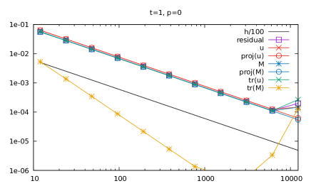
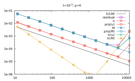
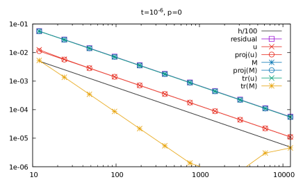
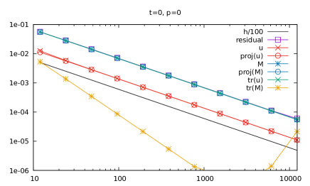
Figure 1: Errors in the case of piecewise constant approximations, $t=1,10^{-3},10^{-6},0$.

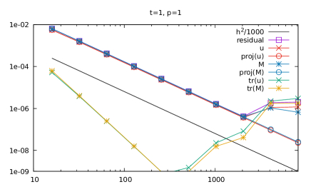
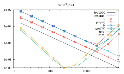
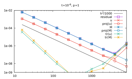
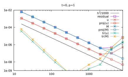
Figure 2: Errors in the case of piecewise linear approximations, $t=1,10^{-3},10^{-6},0$.

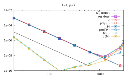
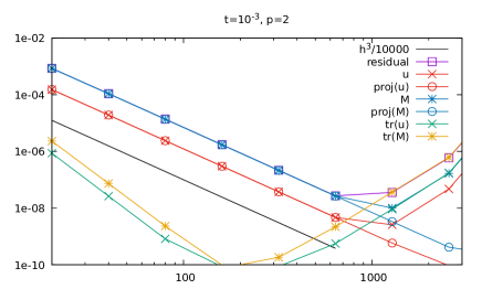
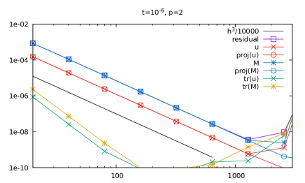
Figure 3: Errors in the case of piecewise quadratic approximations, $t=1,10^{-3},10^{-6},0$.

References

- [1] M. Baccouch, The local discontinuous Galerkin method for the fourth-order Euler-Bernoulli partial differential equation in one space dimension. Part I: Superconvergence error analysis, J. Sci. Comput., 59 (2014), pp. 795–840.
- [2] C. Carstensen, L. F. Demkowicz, and J. Gopalakrishnan, Breaking spaces and forms for the DPG method and applications including Maxwell equations, Comput. Math. Appl., 72 (2016), pp. 494–522.
- [3] F. Celiker, B. Cockburn, and H. K. Stolarski, Locking-free optimal discontinuous Galerkin methods for Timoshenko beams, SIAM J. Numer. Anal., 44 (2006), pp. 2297–2325.
- [4] J. Chan, N. Heuer, T. Bui-Thanh, and L. F. Demkowicz, Robust DPG method for convection-dominated diffusion problems II: Adjoint boundary conditions and mesh-dependent test norms, Comput. Math. Appl., 67 (2014), pp. 771–795.
- [5] L. F. Demkowicz, T. Führer, N. Heuer, and X. Tian, The double adaptivity paradigm (How to circumvent the discrete inf-sup conditions of Babuška and Brezzi), ICES Report 19-07, The University of Texas at Austin, 2019.
- [6] L. F. Demkowicz and J. Gopalakrishnan, Analysis of the DPG method for the Poisson problem, SIAM J. Numer. Anal., 49 (2011), pp. 1788–1809.
- [7] L. F. Demkowicz and N. Heuer, Robust DPG method for convection-dominated diffusion problems, SIAM J. Numer. Anal., 51 (2013), pp. 2514–2537.
- [8] T. Führer, A. Haberl, and N. Heuer, Trace operators of the bi-Laplacian and applications, IMA J. Numer. Anal. (accepted for publication), arxiv:1904.07761.
- [9] T. Führer and N. Heuer, Fully discrete DPG methods for the Kirchhoff–Love plate bending model, Comput. Methods Appl. Mech. Engrg., 343 (2019), pp. 550–571.
- [10] T. Führer, N. Heuer, and A. H. Niemi, An ultraweak formulation of the Kirchhoff–Love plate bending model and DPG approximation, Math. Comp., 88 (2019), pp. 1587–1619.
- [11] T. Führer, N. Heuer, and F.-J. Sayas, An ultraweak formulation of the Reissner–Mindlin plate bending model and DPG approximation, Numer. Math. (accepted for publication), arxiv:1906.04869.
- [12] N. Heuer and M. Karkulik, A robust DPG method for singularly perturbed reaction-diffusion problems, SIAM J. Numer. Anal., 55 (2017), pp. 1218–1242.
- [13] F. Lepe, D. Mora, and R. Rodríguez, Locking-free finite element method for a bending moment formulation of Timoshenko beams, Comput. Math. Appl., 68 (2014), pp. 118–131.
- [14] L. K. Li, Discretization of the Timoshenko beam problem by the and the - versions of the finite element method, Numer. Math., 57 (1990), pp. 413–420.
- [15] A. H. Niemi, J. A. Bramwell, and L. F. Demkowicz, Discontinuous Petrov-Galerkin method with optimal test functions for thin-body problems in solid mechanics, Comput. Methods Appl. Mech. Eng., 200 (2011), pp. 1291–1300.