Magnetic field evolution in solar-type stars

Abstract

We discuss selected aspects regarding the magnetic field evolution of solar-type stars. Most of the stars with activity cycles are in the range where the normalized chromospheric Calcium emission increases linearly with the inverse Rossby number. For Rossby numbers below about a quarter of the solar value, the activity saturates and no cycles have been found. For Rossby numbers above the solar value, again no activity cycles have been found, but now the activity goes up again for a major fraction of the stars. Rapidly rotating stars show nonaxisymmetric large-scale magnetic fields, but there is disagreement between models and observations regarding the actual value of the Rossby number where this happens. We also discuss the prospects of detecting the sign of magnetic helicity using various linear polarization techniques both at the stellar surface using the parity-odd contribution to linear polarization and above the surface using Faraday rotation.

1 Introduction

The purpose of this paper is to discuss recent results relevant for understanding the connection between observations and simulations of magnetic fields in solar-like stars. We focus on observational measures of stellar activity, the occurrence of activity cycles in other stars, and new ways of interpreting stellar surface magnetic fields in terms of linear polarization measurements. We also address the possibility of a radial sign reversal of the star’s magnetic helicity some distance above the stellar surface.

The Sun’s magnetic field exhibits remarkable regularity in space and time, as is demonstrated by Maunder’s butterfly diagram (Maunder, 1904). Although comparable diagrams are only now beginning to become possible for other stars (see, e.g., Alvarado-Gómez et al., 2018), there is clear evidence that cyclic chromospheric variability is ubiquitous. This became clear after Wilson (1963, 1978) selected a set of stars that were then monitored for the next three decades at Mount Wilson (Baliunas et al., 1995).

Much of our knowledge on stellar magnetic activity comes from understanding the Sun’s magnetic field. The occurrence of a fairly regular 11-year activity cycle is of course one of its main characteristics. A cycle as clear as that of the Sun has not been observed for any of the other stars monitored so far. The perhaps best observed cycle is that of HD 81809, but that star is a binary and the cyclic component is not a main sequence star, but a subgiant; see Egeland (2018) for a detailed discussion of this interpretation. The lack of equally clear cycles makes one wonder whether the Sun is perhaps a special case. Other evidence in favor of such thinking is the fact that in a diagram of cycle period versus rotation period, the Sun lies right between two different branches, the high and low activity branches (Böhm-Vitense, 2007). There are a few other aspects suggesting that the Sun is special. Some of them are discussed below.

In the earlier work of Brandenburg et al. (1998), which also showed two distinct activity branches, the Sun appeared closer to the inactive branch and not really between two branches. One reason why the Sun was closer to the inactive branch was the fact that they used the 10 year cycle period obtained by Baliunas et al. (1995) for the time interval for which their solar $\langle R^{\prime}_{\rm HK}\rangle$ data were determined from nightly moonlight observations. Using instead the 11 year cycle period determined for the full record since the time of Schwabe (1844) and before (since the time of the Maunder minimum, as was established by Eddy, 1976) yields a position of the Sun that is now further away from the inactive branch (Brandenburg et al., 2017), although it is still not really between the two branches. Regarding the clear cyclicity, it should also be kept in mind that the Sun is relatively old compared with many of the stars for which cycles have been obtained. It is therefore possible that there is some sort of selection effect for why only the Sun has such a well defined cycle.

We begin by discussing first the relation between rotation period and stellar activity. Also this relation suggests that the Sun’s location in that diagram is between two different modes of behavior, which is when the activity attains a minimum as a function of rotation periods. Both for faster and for slower rotation, the activity increases relative to that of the Sun, at least approximately; see the work Brandenburg & Giampapa (2018), who offered an interpretation in terms of the stellar differential rotation changing from solar-like to antisolar-like differential rotation right at the Sun’s rotation rate. So, again, the Sun appears to take a special position among the many other stars. We finish by discussing new ideas for determining solar and stellar magnetic helicity from linear polarization measurements. This technique, however, has so far only been applied to the Sun.

2 Activity versus rotation

Stellar variability is usually characterized by the chromospheric Ca ii H+K line emission, normalized by the bolometric flux and corrected for photospheric contributions to give $R^{\prime}_{\rm HK}$. This quantity is believed to be a good measure of the mean magnetic field normalized by the equipartition field strength, which is defined based on the kinetic energy as $B_{\rm eq}=\sqrt{4\pi\rho}u_{\rm rms}$, where $u_{\rm rms}$ is the rms value of the turbulent velocity and $\rho$ is the local gas density. Schrijver et al. (1989) estimated that $R^{\prime}_{\rm HK}$ is related to the rms magnetic field strength, $B_{\rm rms}$, through

$$R^{\prime}_{\rm HK}\propto(B_{\rm rms}/B_{\rm eq})^{0.5},$$ (1)

where $B_{\rm rms}$ is expressed in terms of a filling factor $f$ and the typical field strength in spots $B_{\rm spot}$, which can be estimated by the photospheric pressure $p_{\rm phot}$ as $B_{\rm spot}=\sqrt{8\pi p_{\rm phot}}$. Saar & Linsky (1985) thus proposed

$$B_{\rm rms}=f\,B_{\rm spot}.$$ (2)

As stars become more active, $f$ increases up to the point when the entire stellar surface is covered with spots, leading to saturation as $f$ cannot increase beyond unity ($f\leq 1$ by definition).

Stellar rotation with angular velocity $\Omega$ affects the dynamo process through the Coriolis force, $2\bm{\Omega}\times\mbox{\boldmath$u$}{}$, and its strength is characterized by the Coriolis number, $\mbox{\rm Co}=2\Omega\tau$, where $\tau$ is some measure of the turnover time. One often quotes the Rossby number, $\mbox{\rm Ro}=P_{\rm rot}/\tau$, where $P_{\rm rot}=2\pi/\Omega$ is the rotation period. The two parameters are then related to each other through $\mbox{\rm Ro}=4\pi/\mbox{\rm Co}$, although Brandenburg et al. (1998) defined the Rossby number simply as $\mbox{\rm Co}^{-1}$. There are also other reasons why a statement about the Rossby number should be taken with care.

To know the actual values of Ro or Co, one has to agree on a good definition for $\tau$. From an observational point of view, all that matters is that $\tau$ is a monotonically decreasing function of stellar mass, or, in practice, a monotonically increasing function of the color $B-V$. But even then there can be significant uncertainties. In the relevant color range of $B-V$ between 0.6 and 0.75, the turnover times of Barnes & Kim (2010) are about 2.4 times longer than those of Noyes et al. (1984a). In the work of Brandenburg & Giampapa (2018), for example, the turnover times of Noyes et al. (1984a) were adopted. For definitiveness, we refer to those times as $\tau_{\rm Noy}$. The original calculation of $\tau_{\rm Noy}$ was based upon stellar mixing length models of Gilman (1980), where $\tau_{\rm Noy}=\ell/u_{\rm rms}$ was based on the local mixing length $\ell$ and the rms velocity $u_{\rm rms}$ about one scale height above the bottom of the convection zone.

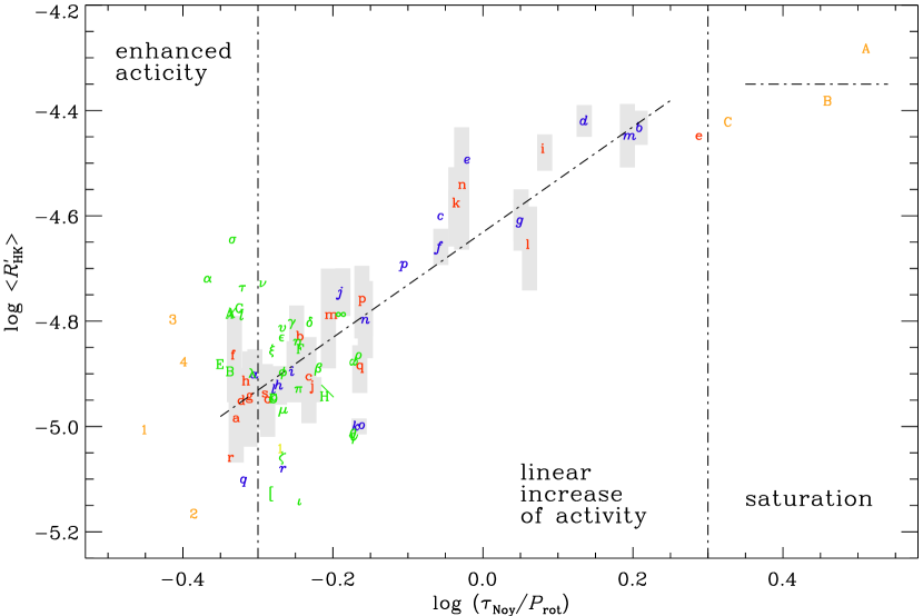
Figure 1: Activity versus Rossby number, showing saturation for $\log(\tau_{\rm Noy}/P_{\rm rot})>0.3$ (see Table LABEL:TSum1) and enhanced activity for many stars in the range $\log(\tau_{\rm Noy}/P_{\rm rot})<-0.3$ (see also Table LABEL:TSum2).

It has been known for some time that $R^{\prime}_{\rm HK}$ scales with Co (Noyes et al., 1984a; Vilhu, 1984) and is therefore inversely proportional to Ro, until saturation is reached for rapid rotation. As alluded to above, saturation is often interpreted in terms of the filling factor of the magnetic field on the stellar surface approaching unity. However, none of the stars with cycles are anywhere near saturation, so they obey $\langle R^{\prime}_{\rm HK}\rangle\propto\mbox{\rm Co}$, but there is some leveling off for non-cyclic stars with $\log(\tau_{\rm Noy}/P_{\rm rot})>0.3$. This is shown in Figure 1, where we have combined data from the three stars of Table LABEL:TSum1 (see the orange labels A–C for HD 17925, 131156A, and 131156B, respectively) with data from Brandenburg et al. (2017), red characters for K dwarfs and blue ones for G and F dwarfs, and Brandenburg & Giampapa (2018), green symbols, for the stars of the open cluster M 67 with rotation periods estimated from gyrochronology based on an estimated age of $4\,{\rm Gyr}$; see Brandenburg & Giampapa (2018) for details. The orange numbers 1–4 for small values of $\log(\tau/P_{\rm rot})$ are for other field stars discussed already in Brandenburg & Giampapa (2018); see also Table LABEL:TSum2. For those stars, we have computed their ages from Equations (12)–(14) of Mamajek & Hillenbrand (2008) as

$$t=\left\{P_{\rm rot}/[0.407\,(B-V-0.495)^{0.325}]\right\}^{1.767},$$ (3)

provided $B-V>0.495$; see also Brandenburg et al. (2017).

Some of the stars of M67 show increasing activity with decreasing $\tau_{\rm Noy}/P_{\rm rot}$ or decreasing rotation rate, which suggests that the activity rises again as they slow down further. This has been interpreted by Brandenburg & Giampapa (2018) as possible evidence for anti-solar differential rotation, which is theoretically expected for very slow rotation (Gilman, 1977). The absolute differential rotation in the regime of antisolar differential rotation is known to be stronger than that in the regime of solar-like differential rotation (Gastine et al., 2014; Käpylä et al., 2014), and also leads to larger magnetic activity for stars with smaller $\tau_{\rm Noy}/P_{\rm rot}$ (Karak et al., 2015), thus explaining their enhanced activity.

Table 1: Parameters of three active stars in the saturation range. The data are taken from Noyes et al. (1984a) and the gyrochronological age is computed from the formula of Mamajek & Hillenbrand (2008); see also Equation (3).

Label HD $B$–$V$ $\tau\;$ [d] $P_{\rm rot}$ [d] $\log\langle R^{\prime}_{\rm HK}\rangle$ Age [Gyr] A 17925 0.87 21.3  6.6 $-4.28$ 0.2 B 131156A 0.76 17.8  6.2 $-4.38$ 0.3 C 131156B 1.17 24.3 11.5 $-4.42$ 0.5

Table 2: Stars in the range of enhanced activity. HD 187013 and HD 224930 do indeed show enhanced activity. For HD 187013, $B-V$ is outside the range of applicability of Equation (3).

Label HD $B$–$V$ $\tau\;$ [d] $P_{\rm rot}$ [d] $\log\langle R^{\prime}_{\rm HK}\rangle$ Age [Gyr] 1 141004 0.60 9.1 25.8 $-5.00$ 5.6 2 161239 0.65 12.0 29.2 $-5.16$ 5.5 3 187013 0.47 3.1  8.0 $-4.79$ old 4 224930 0.67 13.1 33.0 $-4.88$ 6.4

However, when comparing with simulations, the situation is still somewhat puzzling. In fact, numerical simulations of convectively driven dynamo action show that there is another transition, where the large-scale magnetic field becomes predominately nonaxisymmetric with an $m=1$ azimuthal modulation (Viviani et al., 2018). Present models show that these two transitions happen more or less at the same value of Co, but observations shows that the two transitions happen at different values: anti-solar differential rotation for $\mbox{\rm Ro}\mathrel{\mathchoice{\vbox{\offinterlineskip\halign{\hfil$\displaystyle#$\hfil\cr>\cr\sim\cr}}}{\vbox{\offinterlineskip\halign{\hfil$\textstyle#$\hfil\cr>\cr\sim\cr}}}{\vbox{\offinterlineskip\halign{\hfil$\scriptstyle#$\hfil\cr>\cr\sim\cr}}}{\vbox{\offinterlineskip\halign{\hfil$\scriptscriptstyle#$\hfil\cr>\cr\sim\cr}}}}2.0$ (Brandenburg & Giampapa, 2018) and nonaxisymmetric large-scale field for $\mbox{\rm Ro}\mathrel{\mathchoice{\vbox{\offinterlineskip\halign{\hfil$\displaystyle#$\hfil\cr<\cr\sim\cr}}}{\vbox{\offinterlineskip\halign{\hfil$\textstyle#$\hfil\cr<\cr\sim\cr}}}{\vbox{\offinterlineskip\halign{\hfil$\scriptstyle#$\hfil\cr<\cr\sim\cr}}}{\vbox{\offinterlineskip\halign{\hfil$\scriptscriptstyle#$\hfil\cr<\cr\sim\cr}}}}0.5...1.0$; see Table 5 of Viviani et al. (2018), who refer to data of Lehtinen et al. (2016). In fact, recent work of Lehtinen et al. (2020) suggests that the transition from nonaxisymmetric to axisymmetric magnetic fields might be accompanied a change in the slope of the chromospheric activity versus Rossby number diagram, which becomes particularly clear when they combine data of main sequence stars with those of subgiants and giants. The lack of corresponding features in data from numerical simulations is an important shortcoming of current simulations. It could be that some sort of “renormalization” is required when comparing numerical simulations with observational data. Indeed, simulations are long known to yield cyclic behavior only for rotation rates that exceed the solar value by about a factor of three (Brown et al., 2011).

Not all stars necessarily slow down with age. Their Sun-like activity cycles may just disappear, but they would still spin rapidly (Metcalfe & van Saders, 2017). If their magnetic field topology develops predominantly small scales, as has now been demonstrated by Metcalfe et al. (2019), magnetic breaking would become progressively inefficient. This idea emerged when discrepancies between helioseismic ages and gyrochronological ages became apparent (van Saders et al., 2016). Brandenburg & Giampapa (2018) speculated that this could still be reconciled with the possibility of antisolar differential rotation if there is a bifurcation into two possible scenarios: stars that make the transition to antisolar differential rotation as a result of a sufficiently chaotic evolution, and others that just change their field topology and remain rapidly spinning. Demonstrating this with actual models would clearly be a next important step.

3 Cycle frequency versus activity

A systematic dependence of cycle frequency $\omega_{\rm cyc}$ ($=2\pi/P_{\rm cyc}$) on rotation rate $\Omega$ was first found by Noyes et al. (1984b) based on the early analyses of the sample of Wilson (1963, 1978) measured at Mount Wilson. They found $\omega_{\rm cyc}\propto\Omega^{1.25}$. It is important to emphasize that the exponent is larger than unity, which has long been a theoretical difficulty to explain. An early theoretical analysis by Kleeorin et al. (1983) based on the fastest growing linear eigenmode yielded promising results with $\omega_{\rm cyc}\propto\Omega^{4/3}$, but very different solutions were obtained for nonlinear saturated dynamos (Tobias, 1998). This was also emphasized by Brandenburg et al. (1998), who proposed that spatial nonlocality could be strong enough so that only solutions with the lowest wavenumber would exist. This seems to be the best explanation even today.

Table 3: Selected stars with well defined cycles using data from Brandenburg et al. (2017).

Label HD $B$–$V$ $\tau\;$ [d] $P_{\rm rot}$ [d] $\log\langle R^{\prime}_{\rm HK}\rangle$ Age [Gyr] $P_{\rm cyc}$ [yr] comp a (blue) Sun 0.66 12.6 $25.4$ $-4.90$ 4.6 $11.0$  6.6 c (blue)   10476 0.84 20.6 $35.2$ $-4.91$ 4.9 $~{}9.6$  9.3 f (blue)   26965 0.82 20.1 $43.0$ $-4.87$ 7.2 $10.1$ 10.9 m (blue) 160346 0.96 22.7 $36.4$ $-4.79$ 4.4 $~{}7.0$  8.5

As already mentioned in the introduction, there are only very few stars that show well defined cycles that are nearly as clean as that of the Sun. We have listed the properties of these stars in Table LABEL:TSum3, where we also list the cycle periods, $P_{\rm cyc}$, as well as those computed from the formula of Brandenburg et al. (2017) that assumes that the stars lie exactly on the long-period branch. The stars cover the full range in $\log(\tau_{\rm Noy}/P_{\rm rot})$ from $-0.3$ to $0.2$; see Figure 1. The ages of those stars are in the range from $4.4$ to $4.9\,{\rm Gyr}$, except for HD 26965, which is $7.2\,{\rm Gyr}$. This shows that all stars with well defined cycles are old stars.

Furthermore, the analysis of many cycle data by Baliunas et al. (1995) suggested the existence of multiple cycles. Their reality remains debated even today (Boro Saikia et al., 2016; Olspert et al., 2018). The work of Brandenburg et al. (1998) and Brandenburg et al. (2017) suggested two nearly parallel branches of values of $\omega_{\rm cyc}/\Omega$ versus $\langle R^{\prime}_{\rm HK}\rangle$. The lower branch has cycle periods that are about six times longer than those on the regular (upper) branch, where also the Sun was thought to be located, if we adopted the $10\,{\rm yr}$ period; see the discussion above. The two branches were originally called active and inactive branches, because they were also well separated with respect to the vertical line $\lg\langle R^{\prime}_{\rm HK}\rangle=-4.65$. Brandenburg et al. (2017) suggested, however, that (i) the branches are now well overlapping and that (ii) stars younger than $3\,{\rm Gyr}$ might exhibit both shorter and longer cycles simultaneously. It should be remembered that these stars tend to be rapid rotators, whose large-scale magnetic field is expected to be nonaxisymmetric (Viviani et al., 2018). Such a magnetic field is similar to that of a dipole lying in the equatorial plane and with opposite polarities at longitudes that are $180\hbox{${}^{\circ}$}$ away from each other.

Nonaxisymmetric magnetic fields have long been predicted based on mean-field models with an anisotropic $\alpha$ effect, and a tensor $\alpha_{ij}$ whose diagonal components do not all have the same value. Since the early work of Rüdiger (1978), it was known that at rapid rotation, $\alpha_{ij}$ attains an additional piece proportional to $\Omega_{i}\Omega_{j}$, so the tensor approaches the form

$$\alpha_{ij}\to\alpha_{0}\Big{(}\delta_{ij}-\Omega_{i}\Omega_{j}/\Omega^{2}\Big{)},$$ (4)

showing that the component of $\alpha$ in the $\bm{\Omega}$ direction vanishes. In other words, if the $\bm{\Omega}$ direction corresponds to the $z$ direction in Cartesian coordinates, $\alpha_{ij}$ is proportional to ${\rm diag}\,{}(\alpha_{xx},\,\alpha_{yy},\,0)$. In general, there can also be off-diagonal components, but those are not important for the present discussion. The main point is that with $\alpha_{zz}=0$, the dynamo-generated magnetic field is, in Cartesian geometry, always horizontal. In a sphere, it then corresponds to a dipole lying in the equatorial plane; see Fig. 3(a) of Moss & Brandenburg (1995).

A simple example of such a field is that generated by the Roberts flow I (the first of four flows I–IV studied by Roberts, 1972). This flow takes the form

$$\mbox{\boldmath$u$}{}=\mbox{\boldmath$\nabla$}{}\times\psi\hat{\mbox{\boldmath$z$}}{}+k_{\rm f}\psi\hat{\mbox{\boldmath$z$}}{},$$ (5)

which is a prototype example for modeling magnetic fields generated by an $\alpha$ effect. Here, the $\alpha$ tensor is indeed of the form of Equation (4) with $\alpha_{ij}={\rm diag}\,{}(\alpha_{0},\,\alpha_{0},\,0)$ and some coefficient $\alpha_{0}$. It is also a model of the magnetic field generated in the Karlsruhe dynamo experiment, which, in turn, is an idealized model of the geodynamo (Rädler et al., 2002; Rädler & Brandenburg, 2003). The Coriolis number of the geodynamo is extremely large—much larger than that of any of the observed stars. It therefore tends to exaggerate the effects of rotation.

Observationally, nonaxisymmetric magnetic fields have been inferred from light curve modeling and Doppler imaging (see, e.g., Kochukhov et al., 2017). However, we also know that stars with nonaxisymmetric magnetic field can exhibit what is known as flip-flop phenomenon (Jetsu et al., 1994). This means that the two opposite polarities alternate in strengths in a cyclic fashion.

It is generally expected that such variations correspond to a mixed parity solution of the type originally investigated by Rädler et al. (1990). Subsequent work of Moss et al. (1995) found it difficult to obtain such solutions with their more realistic simulations. Qualitative discussions have also been offered by Elstner & Korhonen (2005).

Another related question concerns the cycle period observed for stars on the active or long-period branch discussed above. Guerrero et al. (2019a) suggest that some sort of magnetic shear instability might be responsible for cycle periods comparable to those of the Sun. In this connection, there is also the question whether the Tayler instability might play a role; see Guerrero et al. (2019b). An important question concerns the surface appearance of magnetic fields from the two branches of short and long cycle periods, especially for young and rapidly rotating stars. Are they really nonaxisymmetric and how can we understand the observed occurrence of multiple cycles, i.e., the occurrence of multiple branches with the same stars on both of them? Modeling this convincingly would be a major step forward in understanding the truth behind these two branches.

4 New twists to polarimetric measurements

Zeeman Doppler Imaging (ZDI) provides a powerful tool for characterizing the actual magnetic field structure and its temporary changes. Both in solar and stellar physics, one tends to display the results directly in terms of the full magnetic field vector. Those results are in general subject to the $180\hbox{${}^{\circ}$}$ ambiguity, which is also sometimes referred to as the $\pi$ ambiguity. In the solar context, this $\pi$ ambiguity might be an important source of error in calculating the sign of the Sun’s magnetic helicity at large length scales. It may therefore be advantageous to work directly with the Stokes parameters (Brandenburg et al., 2019; Brandenburg, 2019; Prabhu et al., 2020).

Magnetic helicity is a quantity that characterizes the handedness of the magnetic field. Its sign would change if one looked at the star through a mirror. In this connection, it is important to realize that the Stokes $Q$ and $U$ parameters can directly be expressed in terms of a quantity that characterizes the sense of handedness. This technique is routinely employed in cosmology, where one expresses $Q$ and $U$ in terms of what is known as the parity even $E$ and the parity odd $B$ polarizations. To obtain $E$ and $B$, one expands $Q$ and $U$ not in terms of the ordinary spherical harmonics, but in terms of spin-2 spherical harmonics, ${}_{2}Y_{\ell m}(\theta,\phi)$; see Goldberg et al. (1967). One then obtains $E$ and $B$ as the real and imaginary parts of the transformed quantity in the form (Kamionkowski et al., 1997; Seljak & Zaldarriaga, 1997; Zaldarriaga & Seljak, 1997; Durrer, 2008; Kamionkowski & Kovetz, 2016)

$$E+{\rm i}B\equiv R=\sum_{\ell=2}^{N_{\ell}}\sum_{m=-\ell}^{\ell}\tilde{R}_{\ell m}Y_{\ell m}(\theta,\phi),$$ (6)

where the $\tilde{R}_{\ell m}$ are given by

$$\tilde{R}_{\ell m}=\int_{4\pi}(Q+{\rm i}U)\,_{2}Y_{\ell m}^{\ast}(\theta,\phi)\,\sin\theta\,{\rm d}{}\theta\,{\rm d}{}\phi.$$ (7)

In spectral space, we then define $\tilde{E}_{\ell m}=(\tilde{R}_{\ell m}+\tilde{R}_{\ell,\,-m}^{\ast})/2$ as the parity-even part and $\tilde{B}_{\ell m}=(\tilde{R}_{\ell m}-\tilde{R}_{\ell,\,-m}^{\ast})/2{\rm i}$ as the parity-odd part, where the asterisk means complex conjugation. This has recently been done for the Sun’s magnetic field using synoptic vector magnetograms, which yield a global map. It turns out that $E$ is indeed even about the equator and $B$ is odd about the equator. Therefore, $\tilde{E}_{\ell m}$ has contributions mainly from even values of $\ell$ and $\tilde{B}_{\ell m}$ has mainly contributions from odd values of $\ell$. As a useful proxy, one can therefore employ the correlators

$$K_{\ell}^{+}=\tilde{E}_{\ell}\tilde{B}_{\ell+1}^{\ast}\quad\mbox{and}\quad K_{\ell}^{-}=\tilde{E}_{\ell}\tilde{B}_{\ell-1}^{\ast},$$ (8)

respectively, for different values of $\ell$. There have also been attempts to determine the handedness of magnetic fields in the solar neighborhood of the interstellar medium (Bracco et al., 2019).

To illustrate the decomposition further, we now discuss the corresponding Cartesian decomposition. It reads (Durrer, 2008)

$$\tilde{R}(k_{x},k_{y})=-(\hat{k}_{x}-{\rm i}\hat{k}_{y})^{2}\tilde{P}(k_{x},k_{y}),$$ (9)

where

$$\tilde{P}(k_{x},k_{y})=\int P(x,y)e^{-{\rm i}\bm{k}\cdot\bm{x}}{\rm d}{}^{2}x$$ (10)

is the Fourier transform of $P=Q+{\rm i}U$, and $\bm{k}=(k_{x},k_{y})$ $\bm{x}=(x,y)$ are two-dimensional vectors. The return transform, here written for $R$, is given by

$$R(x,y)=\int\tilde{R}(k_{x},k_{y})e^{{\rm i}\bm{k}\cdot\bm{x}}{\rm d}{}^{2}x/(2\pi)^{2}.$$ (11)

To generate a two-dimensional vector field, it suffices to combine the vector $\mbox{\boldmath$b$}{}=(b_{x},b_{y})$ into a single complex field, ${\cal B}(x,y)=b_{x}+{\rm i}b_{y}$. Next, to generate a periodic pattern, we use the complex wavenumber ${\cal K}\equiv k_{x}+{\rm i}k_{y}$ and generate a pattern in Fourier space as the simplest possible nontrivial analytic function, $\tilde{\cal B}({\cal K})={\cal K}$, along with some phase factor $e^{{\rm i}\phi}$ with phase $\phi$; see Figure 2. We also adopt its complex conjugate, ${\cal K}$; see Figure 3. In both cases we normalize by $|{\cal K}|^{3}$ to reduce the values further away from the origin.

Figure 2: Plots of $e^{{\rm i}\pi n/4}(k_{x}+{\rm i}k_{y})/k^{3}$ for $n=0$, 1, 2, and 3. Different values of the phase sample $E$ patterns ($n=0$ and $2$) and $B$ patterns ($n=1$ and $3$) in a continuous fashion.

Figure 3: Plots of $e^{{\rm i}\pi n/4}(k_{x}-{\rm i}k_{y})/k^{3}$ for $n=0$, 1, 2, and 3. Unlike the case with $(k_{x}+{\rm i}k_{y})$, shown in Figure 2, these patterns do not correspond to the usual $E$ or $B$ polarizations.

We see that the different patterns of $\tilde{\cal B}({\cal K})=e^{{\rm i}\phi}{\cal K}$ correspond to qualitatively different patterns. For $n=0$ and 2, we obtain parity-even patterns ($E$ polarizations with different signs of $E$), whereas for $n=1$ and 3, we obtain parity-odd patterns ($B$ polarizations with different signs of $B$). For $e^{{\rm i}\phi}{\cal K}^{*}$, on the other hand, the patterns are quite different, and they correspond to just the inverse of the former ones in the sense that if one multiplies the $\tilde{\cal B}({\cal K})$ of Figure 2 with those of Figure 3, one obtain just the phase of $R=E+{\rm i}B$, so its decomposition into real and imaginary parts returns as the $E$ and $B$ polarizations, as expected from Equation (9).

Before closing, let us mention here one more aspect regarding polarized emission. Normally, Faraday rotation leads to Faraday depolarization, that is, the cancellation of polarized emission from the line-of-sight integration of the intrinsic polarized emission of different orientations. Thus, in galactic magnetic field measurements with radio telescopes, Faraday rotation was long regarded as something “bad”. For a helical field, however, Faraday rotation can also bring some benefits in that it allows us to estimate the sign of magnetic helicity and the approximate length scales of helical magnetic fields. This property was exploited originally in the galactic context (Brandenburg & Stepanov, 2014), but it can probably also be applied to coronal magnetic fields (Brandenburg et al., 2017).

Studying the helicity of coronal magnetic fields further will potentially be extremely useful in order to assess the possibility of a sign reversal of magnetic helicity some distance above the surface of the Sun and of other stars. Such a sign reversal was first noted in the solar wind (Brandenburg et al., 2011), where, far away from the Sun, the typical sign of magnetic helicity was found to be opposite to what it is at a solar surface. This was then later also found in simulations of simple models of global dynamos with a conducting exterior (Warnecke et al., 2011, 2012). Studying and understanding this phenomenon further will be an important aspect of future studies.

5 Discussion

In this work, we have offered some speculation on how stars like the Sun may have evolved from the times they were born to the time when they reached an age beyond that of the present Sun. We expect that the Sun is shortly before changing its rotation from solar-like to antisolar-like differential rotation where the equator rotates slower than the poles; see also Karak et al. (2019) for recent mean-field modeling of such stars. Stars with antisolar differential rotation are also potential candidates for displaying superflares (Katsova et al., 2018). Unfortunately, there is currently no explicit observation of this phenomenon, except for giants (Kővári et al., 2015, 2017). For main sequence stars, this idea is solely based on numerical simulations. It must therefore be hoped that future observations can give us more explicit evidence for this suggestion. Helioseismic techniques might provide one such approach and has already been partially successful (Benomar et al., 2018). Other techniques could involve the measurement of light curves, as has been proposed by Reinhold & Arlt (2015).

We also discussed the need for a better understanding of the cyclic nature of slowly and rapidly rotating stars. Observations are consistent with a magnetic dipole lying in the equatorial plane, but there is also a long-term cyclic variation that could be compatible with the two poles alternating in their relative strengths. But this is not yet borne out by reasonably realistic simulation data.

A promising long-term record of simulation data has been assembled by (Käpylä et al., 2016). Those simulations display a huge variety of different behaviors, including poleward and equatorward migratory patterns, as well as short and long cycle periods, all in one and the same run. It would therefore be useful to produce similar data for stars with different Rossby numbers in an attempt to better understand the various observation signatures, including the various transitions and the proper position of the Sun in this vast parameter space.

Finally, we turned attention to more direct inspection techniques using linear polarization data. This is motivated by the possibility that standard inversion techniques to obtain the magnetic field might be severely flawed by the fact that no safe $\pi$ disambiguation technique exists that tells us whether the magnetic field vector points for forward or backward. This problem results from the fact that polarization “vectors” are not proper vectors as they do not have neither head nor tail. In fact, just to obtain the sign of magnetic helicity, it is, under some conditions, not even necessary to disambiguate the polarization vector. The sign of handedness can in fact be obtained directly from the linear polarization—without resorting to the magnetic field.

An intermediate approach here is to first determine the magnetic field, but then to make it ambiguous again by estimating $Q+{\rm i}U$ from $(b_{x}+{\rm i}b_{y})^{2}$. This sounds somewhat odd, but it has the advantage that one does then not need to worry about wavelength dependencies of the line spectra of Stokes $Q$ and $U$. This has been discussed in detail in the work of A. Prabhu (private communication).

A different approach to using Stokes $Q$ and $U$ directly is in connection with the determination of magnetic helicity in solar and stellar coronae. This idea was originally proposed for edge-on galaxies (Brandenburg & Stepanov, 2014), but it can equally well if he applied to the Sun and other stores. The work of Brandenburg et al. (2017) suggests, however, that one may have a better chance of exploiting this technique by using millimeter wavelengths rather than infrared. In any case, it is necessary to measure polarized intensity over a broad range of different wave lengths. This has now become possible with the emergence of more refined detector technology. In the context of galactic polarization measurements, this technological advance is what led to the development of Faraday tomography (Brentjens & de Bruyn, 2005). This is based on only work of Burn (1966), who recognized that the line-of-sight integral of linear polarization is the same as a Fourier integral and can therefore be inverted, provided one covers a sufficiently broad range of wavelengths. This was exactly the problem that was difficult to overcome in the early days of radio astronomy, where observations could only be carried out in a small number of frequency bands

A reliable measurement of magnetic helicity in the solar corona is greatly helped by the possibility to use the moon as a perfect coronograph. The total eclipse during the IAU symposium has not yet been utilized for that purpose, but this would hopefully change in the near future.

Klaus Strassmeier It is indeed true that we have found no good evidence for anti-solar differential rotation in main sequence stars, but only in giants and subgiants. The stars with anti-solar differential rotation were not solar-like stars when on the main sequence, but may have been some sort of Ap stars without a sign of an outer convection zone. Do we see differential rotation at all in Ap stars? Or, if seen in solar-like main sequence stars, what process switches differential rotation from solar- to anti-solar? Axel Brandenburg The process causing this switching from solar-like to anti-solar differential rotation is an emerging dominance of meridional circulation over the Reynolds stress. Subgiants could also have meridional circulation in a thin outer convective layer causing anti-solar differential rotation.

Christopher Karoff What would happen to the topography of the magnetic field as the stars change to anti-solar differential rotation? Axel Brandenburg According to the simulations, it should be the same, so the magnetic field would still be poleward migrating. This is because in the solar-like differential rotation regime, it has been very difficult to reproduce solar-like equatorward migration. Therefore, poleward migration has been obtained in both cases. In reality, however, this might not be true, and so poleward migration might emerge only with the moment that the star begins to display antisolar differential rotation.

Moira Jardine One of the ways to confuse a periodogram is to have spots whose lifetime is less than the rotation period of the star. Can you say something about any trends in spot lifetime with accuracy? Axel Brandenburg Sunspots are known to have a large range of lifetimes from half a day to three months. Their decay times scale with their surface area, so for the Sun, the larger and more dominant spots do have lifetimes longer than the rotation period.