Exploring Long Tail Visual Relationship Recognition with Large Vocabulary

Abstract

Several approaches have been proposed in recent literature to alleviate the long-tail problem, mainly in object classification tasks. In this paper, we make the first large-scale study concerning the task of Long-Tail Visual Relationship Recognition (LTVRR). LTVRR aims at improving the learning of structured visual relationships that come from the long-tail (e.g., “rabbit grazing on grass”). In this setup, the subject, relation, and object classes each follow a long-tail distribution. To begin our study and make a future benchmark for the community, we introduce two LTVRR-related benchmarks, dubbed VG8K-LT and GQA-LT, built upon the widely used Visual Genome and GQA datasets. We use these benchmarks to study the performance of several state-of-the-art long-tail models on the LTVRR setup. Lastly, we propose a visiolinguistic hubless (VilHub) loss and a Mixup augmentation technique adapted to LTVRR setup, dubbed as RelMix. Both VilHub and RelMix can be easily integrated on top of existing models and despite being simple, our results show that they can remarkably improve the performance, especially on tail classes. Benchmarks, code, and models have been made available at: https://github.com/Vision-CAIR/LTVRR.

1 Introduction

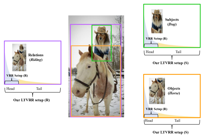
Figure 1: Long-Tail Visual Relationship Recognition (LTVRR). In contrast to existing Visual Relationship Recognition (VRR) setups, where each of the subject (S), objects(O), and relationships (R) have abundant examples, In LTVRR, we focus on such rare relational events where S,R, and O also follow a long-tail distribution which we believe is more realistic and challenging

Most existing works in visual recognition assume that training data are abundant, with typically a few hundred to thousands of examples per class [3, 16, 33, 8, 9]. A more realistic setup, however, is to assume that classes follow a long-tail distribution, where most categories have only few examples. What makes the long-tail distribution more natural is that it covers the spectrum of frequent classes, few-shot classes (classes rarely observed in the training set) and even zero-shot classes (classes that do not appear in the training set). Few-shot and zero-shot learning has been separately studied in [35, 30, 49] and [41, 41, 40], respectively.

LTVRR Several approaches have been developed to advance Long-Tail Object Recognition (LTOR) [20, 22, 39, 36]. However, most of the metrics and evaluation setups in long-tail object recognition do not apply to the Visual Relationship Recognition (VRR) literature, which is more complex and structured. The goal of the VRR task is to recognize the categories of two interacting objects and their relation, e.g., recognizing triplets like $<$dog, riding, horse$>$ [23, 28, 47]. In contrast to most existing VRR benchmarks, all object categories no matter their frequency contribute equally to evaluation metrics in LTOR, where the average per class accuracy is the common metric. Inspired by LTOR literature, we extend their long-tail setup to study visual relationship recognition. In our setup, dubbed Long-Tail Visual Relationship Recognition (LTVRR), subjects, objects, and relationships follow a long-tail distribution; see Fig 1. In this setup, this structured recognition task is more challenging as not only could the combination (S, R, O) be rare, but so can any of the interacting subjects/objects (S/O) and/or the relation (R). An important distinction between our and previous works is that our focus is on much more long-tailed distributions than previous methods. Most long-tail literature focuses on the range of class frequency that it is on a smaller scale than in our setup (between $5$ and $5000$ for  [22], between $1$ and $1000$ for [23], and which is around a factor of $1000$ between the most frequent and the least frequent classes). On the other hand, for our benchmarks, we use the following range of frequencies: For GQA-LT ( $1,703$ object classes and $310$ relation classes), the most frequent object and relationship categories have $374,282$ and $1,692,068$ examples, and the least frequent have $1$ and $2$ examples, respectively. This results in factors of around $300,000+$ for objects and around $1.7$ million for relations between the most frequent and least frequent classes. For VG8K-LT ($5,330$ objects classes and $2000$ relation classes), the most frequent object and relationship categories have $196,944$ and $618,687$ examples, and the least frequent have $14$ and $18$ examples, respectively, which leads to factors of approximately $14,000$ for objects and $34,000$ for relations; see more details in Sec. 4

We also implement several state-of-the-art models [36, 20, 13, 22] targetted on long-tail object classification in our LTVRR setup, which we believe is crucial for further work on this setup. Orthogonally, we also propose a novel augmentation technique, dubbed RelMix and a hubless regularization loss, introduced in section 3. Inspired from [38], in RelMix, we augment the training data systematically using a combination of features to improve upon the tail performance. This effectively helps in augmenting more data for tail classes, hence balancing the head and tail distribution. We also regularize the model by casting long-tail visual understanding as a hubness problem and introduce a Visio-linguistic Hubless (VilHub) loss. The approach is inspired by hubness literature in Natural Language Processing (e.g., [10, 18]) but differs in (a) they use the hubness to improve word-level translation from one language to another, at the same time we model hubness in a visio-lingual task connecting vision to language. (b) Our approach can correct learning representation that minimizes hubness from deep vision and language neural networks in an end-to-end way in contrast to only correcting bias parameters [10].

Contributions:
(1) We adapt several state of the art approaches in long-tail classification to our setup and report the performances on two proposed benchmarks GQA-LT and VG8K-LT. Due to the large vocabulary size of objects and relationships in the LTVRR setup, we also analyze the models based on their capacity to bring categories that are semantically similar to the ground-truth, higher in the rank of the model’s predictions according to wordNet [26], and word2vec [48]. We found this to be useful, especially when the vocabulary of predictions is large.
(2) We propose a novel augmentation method, dubbed RelMix, for the visual relationship recognition problem. We empirically show that our augmentation method, while simple, effectively improves the performance across the whole class distribution with more focus on tail classes.
(3) We propose to cast the long-tail visual understanding as a hubness problem, and introduce a Visio-linguistic Hubless (VilHub) loss.We showed that VilHub loss can be simply integrated with some existing losses like Focal Loss (FL) [20] and Weighted Cross Entropy [20] to improve performance as an effective regularizer.

2 Related Work

Visual Relationship Detection Visual relationship detection (VRD) has been extensively studied in the past few years [23, 46, 42, 23]. Lu et.al. [23] utilizes the object detection output of an R-CNN detector and leverages language priors for relationship prediction.  [48] allows for the visual and language features of the subjects, objects, and relations to be adapted into a common embedding space using a visual and language embedding sub-networks. This was shown to make the model more expressive and outperform previous approaches, such as knowledge distillation [43], ViP-CNN [19], and [28]. [17] introduced a long-tailed dataset with $600$ objects and $57$ relations. Our benchmarks focus on much larger vocabularies (see Sec. 4.1).

Long-tail Classification Long-tail classification has been extensively studied in the literature [7, 2, 32, 31, 50, 1, 21, 51, 27]. Focal loss [20] down-weights the loss assigned to well-classified examples which guides the optimizer to attend more to tail classes which are likely not well classified. In [22] the authors utilize a dynamic visual memory module and a modulated attention mechanism for generalizing over tail classes. In [13], the authors decouple the representation learning from classifier learning and show huge improvements on long-tail classification. Similar to weighted CE Loss, in [36], the authors propose an equalization loss that blocks out gradients from affecting rare classes when training frequent classes, which improved the performance on rare classes. In contrast, we improve the performance on tail classes by our RelMix augmentation strategy and VilHub regularizer.

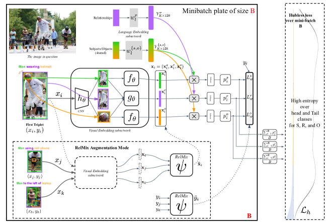
Figure 2: Approach Overview: s-r-o triplets (extracted from the same image) are passed through the visual embedding network, the resultant embeddings are augmented by our method using a combination of features individually from subject, object, and relations. The training is then regularized with ViLub Loss and RelMix augmentation as illustrated.

Augmentation There has been much work [44, 45, 38, 4, 24] in recent years on using augmented data to target better generalization for classification problems. One of the better-known techniques, Mixup  [45], trains a neural network on convex combinations of pairs of examples and their labels. Manifold Mixup [38] builds up on Mixup by using combination of image features rather than raw images for their augmentation technique. Cumix [24] proposes an extension of the Mixup technique to have combination between pairs belonging to different domains for better performance in domain generalization and zero-shot tasks. We propose an augmentation technique inspired by Manifold Mixup for our LTVRD setting for a better generalization on the whole frequency band (many, med, few) of classes, with a special focus on tail classes.

3 Approach

In a visual relationship $<s,r,o>$, we define ${\textbf{x}^{s}},{\textbf{x}^{o}},{\textbf{x}^{r}}$:

$$\small\begin{split}{\textbf{x}^{s}}&=f(h(x^{s}),b^{s})\\ {\textbf{x}^{o}}&=f(h(x^{o}),b^{o})\\ {\textbf{x}^{r}}&=g(h(x^{r}),b^{r},b^{s},b^{o})\\ \end{split}$$ (1)

Where $x^{s}$, $x^{r}$, and $x^{o}$ are the cropped image regions of the subject $s$, relationship $r$, and the object $o$. $b^{r}$, $b^{s}$, and $b^{o}$ are the corresponding bounding boxes. ${\textbf{x}^{s}},{\textbf{x}^{o}},{\textbf{x}^{r}}$ are the transformed embeddings of $x^{s}$, $x^{r}$, and $x^{o}$ respectively with corresponding labels are $y^{s}$, $y^{r}$, and $y^{o}$. $h(\theta)$ consists of the first 5 layers of VGG16, it takes the cropped image regions as input and outputs the visual features. $f(\theta)$ and $g(\theta)$ are neural networks that extract the visual embeddings from the visual features; see Fig. 2.

3.1 Loss Function

Per-example Loss. Given a set of each positive visual-language pair by $(\textbf{x}^{l},\textbf{y}^{l})$, where $l\in\{s,r,o\}$, represented by the aforementioned neural networks, joint vision-language embeddings can be learned by a traditional triplet loss (e.g., [14, 37, 6]). The triplet loss encourages matched embeddings from the paired modalities to be closer than the mismatched ones by a margin $m$. The triplet loss, however, does not sense a learning signal beyond the margin, and the trained model will not learn to distinguish different classes enough for a classification-oriented task. To alleviate this problem,  [48] recently studied a Softmaxed version of the triplet loss for VRR achieving state-of-the-art results. Triplet Softmax loss can be defined as follows (we drop the superscript $l\in\{s,p,o\}$ in this section for simplicity):

$$\small\begin{split}{L}(\textbf{x}_{i},\textbf{y}_{i})&=\frac{1}{N}\sum_{i=1}^{N}-\log\big{(}p_{i}=\frac{e^{\textbf{x}_{i}^{\mathbb{T}}\textbf{y}_{i}}}{e^{\textbf{x}_{i}^{\mathbb{T}}\textbf{y}_{i}}+\sum_{j=1}^{K}e^{\textbf{x}_{i}^{\mathbb{T}}\textbf{y}_{ij}^{-}}}\big{)}\\ &=\frac{1}{N}\sum_{i=1}^{N}-\log\big{(}p_{i}=\frac{e^{\textbf{x}_{i}^{\mathbb{T}}\textbf{y}_{i}}}{\sum_{j=1}^{K}e^{\textbf{x}_{i}^{\mathbb{T}}\textbf{y}_{j}}}\big{)}\end{split}$$ (2)

Where $N$ is the number of positive ROIs. For each positive pair $(\textbf{x}_{i},\textbf{y}_{i})$ and its corresponding set of negative pairs $(\textbf{x}_{i},\textbf{y}_{ij}^{-})$, the similarities between each of them is computed with dot product and then put into a softmax layer followed by multi-class logistic loss so that the similarity of positive pairs would be pushed to be $1$, and $0$ otherwise. In Eq. 2, we show that triplet softmax can be simplified in a form that is very similar to MCE loss if all the other classes except the ground truth are considered negative. We adopted a weighted version of this visiolingual loss, where we allow each class to have a weight $w_{i}$, this weight can be assigned higher values to less frequent classes (e.g., inverse the frequency of the object/relation class); see Eq. 3.

$$\begin{split}{L}_{w}(\textbf{x}_{i},\textbf{y}_{i})=\frac{1}{N}\sum_{i=1}^{N}-w_{i}\log\big{(}p_{i}=\frac{e^{\textbf{x}_{i}^{\mathbb{T}}\textbf{y}_{i}}}{\sum_{j=1}^{K}e^{\textbf{x}_{i}^{\mathbb{T}}\textbf{y}_{j}}}\big{)}\end{split}$$ (3)

VilHub Per-minibatch Loss: Recent NLP approaches like [29, 5, 34] observed that the accuracy of bidirectional retrieval across languages is often significantly degraded by a phenomenon called hubness, which appears when some frequent words, called hubs, get indistinguishably close to many other less represented words. In long-tail VRR context, these hubs are the head classes, which are often over-predicted at the expense of tail classes. To alleviate the hubness phenomenon, we develop a vision $\&$ language hubless loss (dubbed VilHub). Our approach alleviates the long-tail problem by correcting both the language and visual representations in an end-to-end manner. The key idea of our VilHub loss $\mathcal{L}_{\mathbf{h}}$ is to encourage fair prediction over both head and tail classes in the current batch. $\mathcal{L}_{\mathbf{h}}$ is defined as:

$$\small\begin{split}\mathcal{L}_{\mathbf{h}}&=\sum_{i=1}^{K}(pf(\textbf{y}_{i})-\frac{1}{K})^{2},\\ pf(\textbf{y}_{i})&=\frac{1}{B}\sum_{j=1}^{B}\frac{e^{\textbf{x}_{j}^{\mathbb{T}}\textbf{y}_{i}}}{\sum_{k=1}^{K}e^{\textbf{x}_{j}^{\mathbb{T}}\textbf{y}_{k}}}\\ \end{split}$$ (4)

Where $B$ is the mini-batch size, $K$ is the number of classes. The VilHub loss $\mathcal{L}_{\mathbf{h}}$ encourages all the classes (head and tail) to be equally preferred. To achieve this behavior, we define the preference of every class as $pf(\textbf{y}_{i})$ as the average probability of the class being predicted in the current minibatch of size $B$, as shown in Fig. 2. Then, we simply encourage this marginal probability to be close to uniform (i.e., equally preferred across head and tail).

Our Final Loss. In conclusion, our final loss is defined as:

$$\small\begin{split}\mathcal{L}=\frac{1}{B}\sum_{i=1}^{B}{L}_{w}(\textbf{x}_{i},\textbf{y}_{i})+&\gamma\mathcal{L}_{\mathbf{h}},\end{split}$$ (5)

where $\gamma$ is the VilHub loss weight or scale. The first term ${L}_{w}$ encourages the examples to be discriminatively classified correctly in the visual-language space. The second term $\mathcal{L}_{\mathbf{h}}$ encourages a fair prediction over head and tail classes.

3.2 RelMix Augmentation

We denote the input image as $x$, where there exists a visual relationship between subject $s$ and object $o$ with relationship $r$. A visual embedding network processes the image to output three visual embeddings ($\textbf{x}^{s},\textbf{x}^{r},\textbf{x}^{o}$) with corresponding ground truth labels as ($y^{s}$, $y^{r}$, $y^{o}$) for subject, relationship and object. Our RelMix algorithm augments the training data by using a combination of these features in a systematic way to help target the tail classes in the dataset.

RelMix. The goal of RelMix augmentation is to enrich training coverage of visual relationship labels by combining the extracted visual features generated in a meaningful way. During training, three triplets are selected $\textbf{x}_{i}=(\textbf{x}_{i}^{s},\textbf{x}_{i}^{r},\textbf{x}_{i}^{o}$), $\textbf{x}_{j}=(\textbf{x}_{j}^{s},\textbf{x}_{j}^{r},\textbf{x}_{j}^{o}$), $\textbf{x}_{k}=(\textbf{x}_{k}^{s},\textbf{x}_{k}^{r},\textbf{x}_{k}^{o}$)) with corresponding labels ($y_{i}=(y_{i}^{s},y_{i}^{r},y_{i}^{o}),y_{j}=(y_{j}^{s},y_{j}^{r},y_{j}^{o}),y_{k}=(y_{k}^{s},y_{k}^{r},y_{k}^{o})$). We sample these triplets such that ($y_{i}$ and $y_{j}$) belong to the tail/medium classes (high class frequency domain) while the triplet ($y_{k}$) belongs to the tail class ( low class frequency domain). Then inspired from existing augmentation strategies (e.g., [38]), we combine the the input embeddings and corresponding predictions as in Eq. 6.

$$\tilde{\textbf{x}}=\psi(\textbf{x}_{i}^{l},\textbf{x}_{j}^{l},\textbf{x}_{k}^{l})=\lambda\textbf{x}_{i}^{l}+(1-\lambda)(\alpha\textbf{x}_{j}^{l}+(1-\alpha)\textbf{x}_{k}^{l})$$ (6)

$$\tilde{y}=\psi(y_{i}^{l},y_{j}^{l},y_{k}^{l})=\lambda y_{i}^{l}+(1-\lambda)(\alpha y_{j}^{l}+(1-\alpha)y_{k}^{l})$$

Where $l\in\{s,r,o\}$, $\alpha$ is sampled from Bernoulli distribution with probability 0.5, and $\lambda\in[0,1]$. This allows our method to focus on long-tail classes more since the three triplets are chosen in a way to have the augmented features resemble closely to tail ones. The frequent classes are sampled in one out of three triplets to maintain representation quality while the aforementioned VilHub loss encourages fair prediction over all head and tail classes; (see Fig.2).

While RelMix is inspired from Manifold mixup [38], with its augmentation being done at the feature representation level, there are some key differences, (1). Manifold mixup operates on object recognition setting ( one object / image), compared to VRD setting where mini-batches consist of scenes; each having multiple objects and structured relations. (2). Manifold Mixup extracts the (object, label) pairs from many different images, which is not so practical in the VRD setting. We instead extract augmentation tuples of s-r-o triplets from the same scene, so the training efficiency is not significantly hurt. Concretely, we augment the most frequent classes with the least frequent ones in the same scene and vice versa. Further comparison between RelMix and Manifold Mixup is taken up in Section 4.3.

Augmentation Loss. Once $\tilde{\textbf{x}}$ and $\tilde{y}$ is computed, they are then fed to our final loss, defined in Eq. 5.

4 Experiments

4.1 Datasets and Comparison Models

We present experiments on two LTVRR benchmarks that we built on top of Visual Genome [15, 48] and GQA dataset [11] (also based on VG). Both datasets naturally have a long-tail distribution yet only high frequency subjects, relations, and objects are mainly used in the literature.

GQA-LT. We used the visual relationship notations provided with the GQA dataset [11]. The main filtration we applied to GQA data was to remove the objects that did not belong to a subject-relation-object triplet. The resulting benchmark has $72,580$ training images, $2,573$ validation images, and $7,722$ test images; with $1,703$ objects and $310$ relations. We call this version GQA-LT. Most frequent object and relation has $374,282$ and $1,692,068$ examples, and the least frequent are $1$ and $2$, respectively.

VG8K-LT We used the latest version of Visual Genome (VG v1.4) [15] that contains $108,077$ images with $21$ relationships on average per image. We used the data split in  [48] which has $103,077$ training images and $5,000$ testing images following [12] and used the class labels that have corresponding word embeddings [25].

We selected the most frequent $5,330$ object classes out of the original $53,304$ and $2,000$ relationships out of the original $29,086$ to make a cleaner version of VG80K (noisy). The resulting dataset has $97,623$ training images, $1,999$ validation images, and $4,860$ testing images. After the filtration the least frequent object and relation classes have $14$ and $18$ examples, and the most frequent are $196,944$ and $618,687$, respectively, meaning the distribution is very long-tailed. We call this version VG8K-LT.

Table 1: Average per-class accuracy on GQA-LT

	Subject/Object				Relation
Loss	many	medium	few	all	many	medium	few	all
	86	255	1,362	1,703	16	46	248	300
CE [48]	68.3	37.0	6.9	14.5	62.6	15.5	6.8	11.0
CE + VilHub	68.6	44.0	10.3	18.3	63.6	17.6	7.2	11.7
CE + VilHub + RelMix	68.8	42.1	10.1	18.1	63.4	14.9	8.0	11.9
Focal Loss [20]	68.2	39.2	7.5	15.3	60.4	15.7	7.7	11.6
Focal Loss + VilHub	69.0	43.4	9.5	17.5	63.1	14.2	7.5	11.4
OLTR [22]	68.2	37.2	7.0	14.6	62.3	15.8	6.6	10.8
OLTR + VilHub	69.1	38.7	7.6	15.2	63.0	16.8	7.3	11.2
DCPL [13]	64.0	35.3	6.4	13.7	61.4	23.6	7.6	12.7
DCPL + VilHub	63.5	39.8	7.5	15.2	58.6	26.1	7.0	12.5
DCPL + VilHub + RelMix	65.7	40	7.8	15.4	58.9	25.7	6.8	12.3
EQL [36]	68.9	43.7	10.0	18.0	63.5	15.0	8.2	12.1
EQL + VilHub	67.7	43.9	11.1	18.7	62.8	15.8	8.9	12.6
EQL + VilHub + RelMix	69.1	44.3	11.3	18.8	64.1	16.4	9.2	12.8
WCE	53.4	42.0	14.0	20.2	53.4	35.1	15.7	20.5
WCE + VilHub	52.0	44.6	16.0	22.1	53.1	39.0	15.8	21.2
WCE + VilHub + RelMix	52.7	45.2	15.7	22	55.1	39.3	15.7	21.1

Table 2: Average per-class accuracy on VG8K-LT

	Subject/Object				Relation
Loss	many	medium	few	all	many	medium	few	all
	267	799	4,264	5,330	100	300	1,600	2,000
CE [48]	57.3	11.1	8.5	11.4	22.2	15.5	12.6	13.5
CE + VilHub	61.6	20.3	10.1	14.2	27.5	17.4	14.6	15.7
CE + VilHub + RelMix	59.5	15.1	10.4	13.6	24.5	16.5	14.4	15.4
Focal Loss [20]	58.1	13.9	8.9	12.1	24.5	16.2	13.7	14.7
Focal Loss + VilHub	60.5	16.7	9.2	12.9	26.7	15.7	13.9	14.8
OLTR [22]	56.8	12.0	9.6	12.3	22.5	15.6	12.6	13.6
OLTR + VilHub	60.4	15.1	9.8	13.1	27.8	16.4	14.4	15.4
DCPL [13]	53.8	5.9	7.9	9.9	34.4	15.4	12.9	14.4
DCPL + VilHub	56.4	7.0	8.2	10.4	35.2	15.3	12.8	14.3
DCPL + VilHub + RelMix	57.6	7.4	8.3	10.5	35.9	15.5	12.8	14.3
EQL [36]	56.9	12.1	10.0	12.7	22.6	15.6	12.6	13.6
EQL + VilHub	60.3	15.0	10.2	13.4	27.9	16.5	14.4	15.4
EQL + VilHub + RelMix	62.1	15.1	10.4	13.6	29.3	16.9	14.3	15.5
WCE	52.8	27.2	10.8	14.5	35.5	24.7	15.2	17.2
WCE + VilHub	52.0	27.9	11.1	14.8	35.2	24.6	15.3	17.2
WCE + VilHub + RelMix	54.2	26.7	10.3	14.1	36.8	25.3	14.2	16.5

Comparison Models. We compare our method with several state-of-the-art approaches that focus on the long-tail [48, 20, 13, 36]. For fair comparisons, we use the same backbone neural network in [48] with all approaches;  [48] is based on VGG16 architecture [33] .
LSVRU [48]: this is the base visio-lingual model with structured visual encoder.
Focal Loss (FL) [20]: A loss used in object detection setting to alleviate the long-tail problem. We integrated FL with LSVRU on each of $s/o,r$ classification heads.

Weighted Cross Entropy (WCE): We use a weighted version of cross-entropy loss. The weight is based on the inverse class frequency, which gives a large weight to rare classes and a small weight to common classes.

Decoupling (DCPL) [13]: This is a state-of-the-art model in long-tail classification that is based on decoupling representation learning phase from classifier learning phase. We applied DCPL in our LTVRR setup similarly.

OLTR [22]: We implemented the visual memory module augmented with modulated attention by [22] into our LTVRR task using  [48] as a backbone model.

EQL [36]: The equalization loss protects the learning of tail classes from being at a disadvantage during the network parameter updating  [36].
Visio-Lingual Hubless (VilHub): Models using our hubless regularizer explained in section 3.1.
RelMix: This is the model using our proposed augmentation strategy explained in section 3.2.

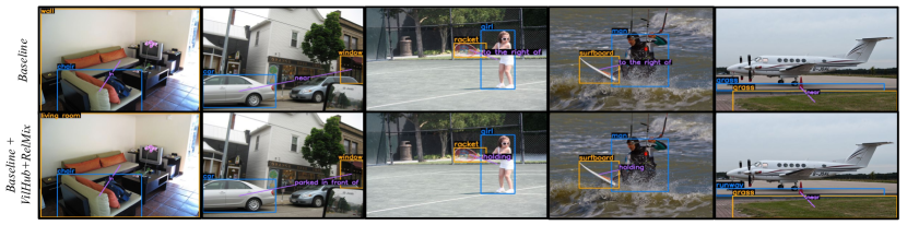
Figure 3: Qualitative examples for our model. In all of these, we see our model preferring the better choice (mostly long-tail) for sbj/obj/rel prediction.

Metrics. Average per-class accuracy The main metric used in the tables is the average per-class accuracy, which is the accuracy of each class calculated separately, then averaged. The average per-class accuracy is a commonly used metric in the long-tail literature [13, 36, 22].

Many, Medium, Few splits: We report the results on the subject, object, and relation separately of an $<$S,R,O$>$ triplet on GQA-LT and VG8K-LT datasets. We evaluate the models using the average per-class accuracy across several frequency bands chosen based on frequency percentiles for GQA-LT: many: top 5% frequent classes, 86 classes for S/O, and 16 classes for R. medium: the middle 15%, 255 classes for S/O, and 46 classes for R. few: the least frequent 80% of classes, 1362 classes for S/O, and 248 classes for R. VG8K-LT is split similarly; see supplementary.

4.2 Quantitative Results

Table 1 shows that adding VilHub loss (w/ and w/o RelMix) to any of the compared models consistently improve their performance on the medium and few classes categories. While VilHub alone can improve almost all the models in med and few categories, we also see the addition of RelMix further improving this in all categories for sbj/obj classification. A similar trend can also be seen when evaluating these models on VG8K-LT dataset, as seen in Table 2.

Comparing LSVRU with and without VilHub in Table 1, VilHub loss improved the performance $\approx$7.0% for sbj/obj medium category, $\approx$3.4% for the sbj/obj few category, and $\approx$2.1% for the relation medium category. In this case, we also see an improvement of $\approx$1.2% on relation few category when combining VilHub with RelMix. We also see a consistent improvement over the whole band (many, med, few) for sbj/obj and rel when using EQL [36] baseline in combination with VilHub and RelMix with a substantial gain of $\approx$6.7% in the med category for relation. A similar improvement in performance with the addition of VilHub (w/ and w/o RelMix) can also be seen in the Decoupling [13], OLTR [22] and Focal Loss [20] baselines. Comparing WCE and WCE + VilHub in sbj/obj branch, we can see that adding the VilHub loss improved $\approx$2% in the few category, and with the addition of RelMix improved $\approx$3.2% in the med category. While similar behavior can be seen in VG8K-LT evaluation (Table 2), we can see that the improvement on GQA-LT is more apparent than on VG8K-LT, since VG8K-LT dataset is more challenging and has more than 5 times the number of objects and more than 7 times the number of relationships compared to GQA-LT. With the model agnostic nature of VilHub+RelMix, they can be easily be integrated on top of existing VRR models to improve their performance, especially on the med and tail categories. Some of the qualitative results can be seen in Figure 3.

4.3 Ablation

Table 3: Ablation Study for RelMix and VilHub.

	Subject/Object				Relation
Model	many	med	few	all	many	med	few	all
LSVRU [48]	68.3	37.0	6.9	14.5	62.6	15.5	6.8	11.0
LSVRU + Manifold Mixup [38]	68	37.5	7.5	15.1	62.4	15.7	6.8	11
LSVRU + RelMix	68.2	37.7	9.3	16.5	62.6	16.0	6.9	11.1
LSVRU - Lang.	68.7	26.0	5.2	11.5	49.9	9.0	5.8	8.5
LSVRU - Lang. + VilHub	69.7	31.4	5.6	12.7	54.1	8.7	5.4	8.4
LSVRU + VilHub(1k)	68.3	37.1	7.0	14.6	63.5	16.3	6.8	11.2
LSVRU + VilHub(5k)	68.4	38.6	7.4	15.2	63.6	17.6	7.2	11.7
LSVRU + VilHub(10k)	68.6	39.7	8.0	15.8	63.6	17.3	7.2	11.6
LSVRU + VilHub(20k)	68.7	41.0	8.4	16.3	63.5	16.5	7.1	11.4

We perform ablations to better understand the influence of the proposed VilHub regularizer and RelMix augmentation; see Table 3. The entry LSVRU + Manifold Mixup represents an adapted version of Manifold Mixup [38] in our setting. We can observe a significant performance gap between the said baseline and RelMix, especially in the few categories of sbj/obj, where the gap is $\approx$1.8%. Further ablations of RelMix augmentation can be found in supp.

The LSVRU - Lang. is our backbone model (LSVRU) without the language guidance network of [48], where we replace it with one FC classification layer. Table 3 shows a drop in performance when removing the language guidance. We also show that VilHub loss worsens the tail relations performance when applied without language guidance.

We further analyze the effect of changing the scale value $\gamma$ (from Eq. 5) of the VilHub regularizer (e.g., 1k, 5k, 10k, 20k). Fig 7 shows that the performance increases on each medium and few classes as we increase the VilHub scale up to an ideal value and then tends to drop. We observe that the ideal VilHub scale value tends to be higher for subjects and objects than for relationships.

4.4 Further Analysis

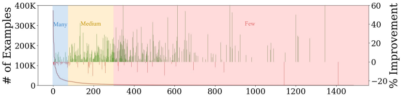
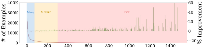
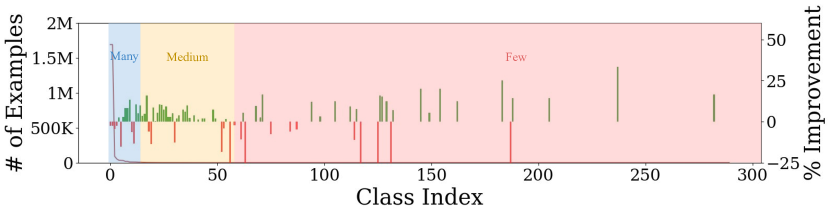
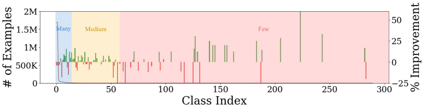
Figure 4: Comparisons of subject/object (upper) and relations (lower) accuracy between LSVRU model with and without VilHub (left) and LSVRU model and LSVRU + RelMix (right) on GQA-LT dataset. The performance for all classes is sorted by frequency. The distribution of classes is shown in the background (in brown). The green are improvement, red bars are worsening, no bars indicate no change. The improvement on the y-axis is the absolute improvement of the classes in percentage accuracy. Note the consistent improvements across tail classes due to VilHub and RelMix

We analyze in more depth the results in Table 1 to better understand the causes of improvements. Figure 4 shows head-to-head comparison between the LSVRU model [48] with and without the VilHub regularizer. For the subjects and objects in Figure 4 (top left), adding the VilHub loss improved 415 classes out of 1703 and only worsened 79 classes. For the relationships Figure 4 (bottom left), adding the VilHub improved 56 classes out of 310 and worsened around 24 classes. The figures show that most of the improvement is over medium and few shot classes (tail). This demonstrates how adding the VilHub loss improves the performances of the classes across the frequency spectrum. On average, we see that VilHub improves many more classes than it worsens and improves more classes on the tail. This confirms our point that adding the VilHub loss as a regularizer in long-tail problems pushes the models to learn classes across the spectrum, and prevents the models from solely focusing on improving the head classes.

Figure 4 (right) shows how adding the Relmix augmentation improves the results across the classes’ spectrum. Figure 4 (top right) shows how consistently RelMix improves the results on the tail end of the distribution (improved around 700 out of 1703 and worsened only 92 classes). Figure 4 (bottom right) shows an overall improvement over the classes with more focus on the tail. This shows our augmentation method’s potential and motivates further research into replicating the consistent improvement on the subjects/objects (Figure 4 top right) to relationships.

In Table 2, we see noticeable performance improvement in the many category aside from the med/few when VilHub is applied. While this result seems surprising at first, we note that by design, our loss encourages the visual classifiers to be more predictive of tail classes while also being accurate on the head. This predictive learning signal helps better leverage tail classes examples contrastively against head classes rather than being ignored. We believe that this enriched contrastive learning of tail classes helps the learning representation of head classes be more discriminative.

We also report our model’s performance using the standard per-example accuracy in Table 4, showing that our proposed models can improve the overall accuracy. However, we may get 90% with the standard accuracy metric if we correctly predict only the top frequent few classes, mostly ignoring the tail. That’s why per-class accuracy is adopted in LTOR literature [13, 36, 22].

Table 4: Average per-example accuracy on GQA-LT

	per-example accuracy
Model	sbj/obj	rel
LSVRU [48]	51.9	94.8
LSVRU + VilHub	53.9	91.2
LSVRU + VilHub + RelMix	53.5	91.0
EQL [36]	51.13	93.85
EQL + VilHub	52.80	92.23
EQL + VilHub + RelMix	52.74	92.58
WCE	37.6	72.6
WCE + VilHub	40.0	74.3
WCE + VilHub + RelMix	47.3	77.6

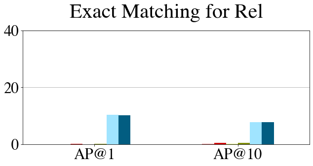
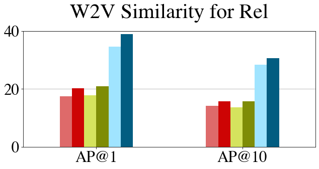
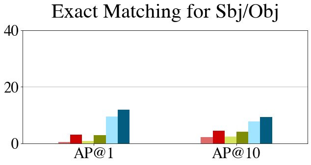
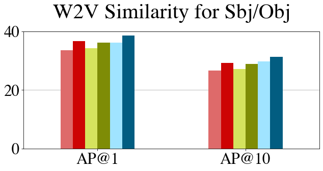
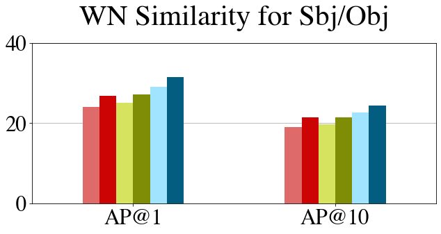
Figure 5: Soft Average Precision calculated on the tail classes on GQA-LT dataset using a variety of metrics. We visualize results using exact similarity metrics, W2V-VG, and average of 6 WordNet metrics. The models using VilHub show consistently superior performance on the tail, when compared to similar models without the VilHub.

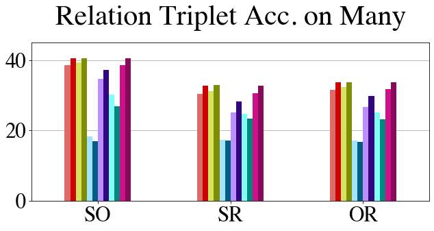
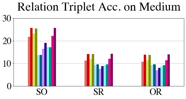
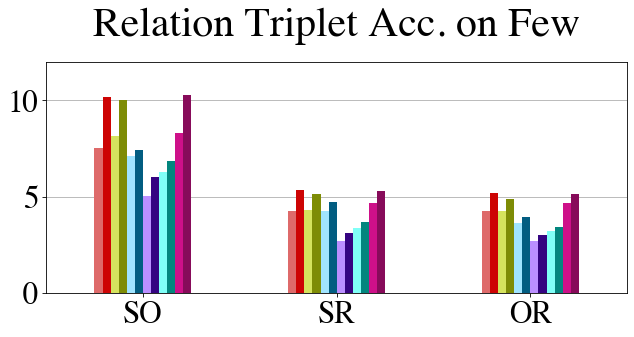
Figure 6: Performance on relationship triplets (S, R, O) grouped by (S, O), (S, R), (O, R) on GQA-LT datasets

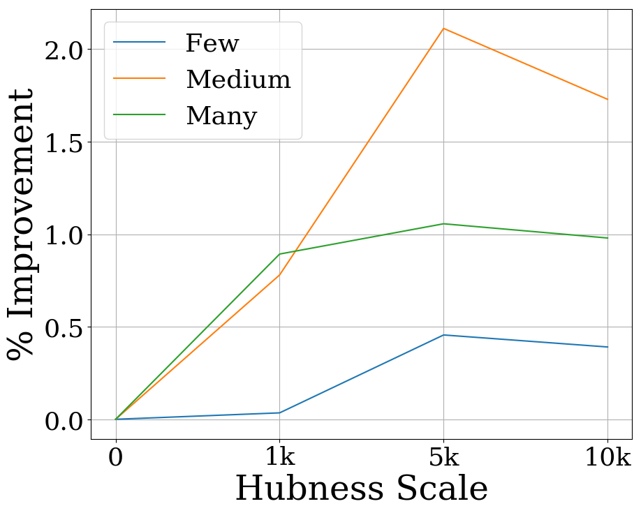
(a) GQA-LT

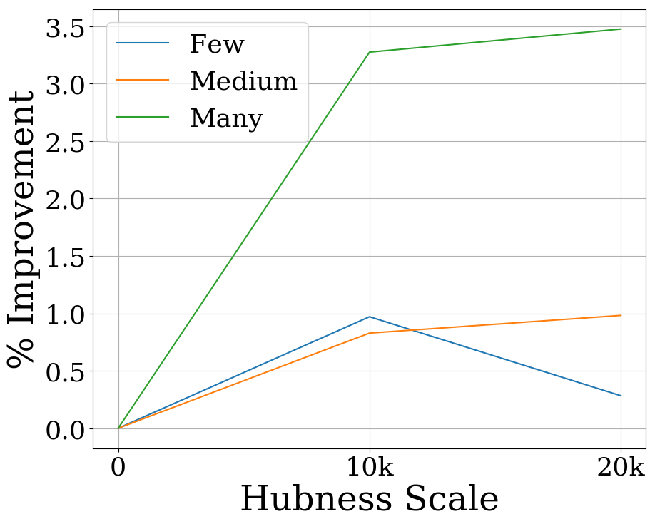
(b) VG-LT

Figure 7: Relationships performance change on the many, medium, few shots classes as we increase the VilHub scale. The performance improves on medium and few (tail) classes up to a certain point and then declines.

4.5 Compositional Results

The long-tail poses a unique problem in relationship recognition due to the combinatorial nature of the problem. dog and motorcycle could be a common subject and object, but they may never be paired with the relationship ride. In LTVRR, the long-tail distribution is not only on subjects, objects, and relations individually but also on their combinations. Meaning, we may not only have a rare combination of classes but also a combination of rare classes (e.g., $<$ otter, riding, dolphin $>$). Here we analyze how the performance is affected by this combinatorial nature of the problem. Fig 6 shows the performance on recognizing the entire triplet (S, R, and O) correctly on GQA-LT, which is the most important metric when evaluating relationship recognition. The results are grouped by pairs of (Subject, Object), (Subject, Relation), and (Object, Relation), and the accuracy is averaged over each group. VilHub improves existing approaches on this angle of performance; we can see in Fig. 6 that the relationship triplet recognition performance is exceeding 40% when we group by pairs of (S, O), while it is under 35% for (S, R) and (O, R). This shows how the more frequent (S,O) is more predictive of the entire triplet’s performance (S,R,O) than other combinations. Fig 6 also shows the superior performance when using VilHub loss ($\approx$ 3% gain ) for most of the models. This shows that VilHub also helps recognizing infrequent combinations of S, R, and O. Additionally, we can see that LSVRU+Relmix+VilHub gives the best performance on the few category ($\approx$11% on SO group) which shows the effectiveness of our augmentation strategy when combined with the VilHub regularizer.

Soft Average Precision Analysis. Fig 5 shows the average precision of our models for the tail classes (least frequent 80%). Concretely, we use the analysis to measure which models bring classes with similar meaning to the ground truth higher in the prediction rank. In agreement with the human subject experiments, the results reveal that all models are doing significantly better than the exact match metric suggests. Another takeaway from this analysis is that similarity metrics trained on relevant data are better at evaluating the models’ performances than metrics trained on less relevant data. This can be seen when comparing the W2V-VG similarity metric (trained on VG) with the other metrics. W2V-VG metric is $\approx$7% more than wordNet metrics and $\approx$10% more than W2V-GN (figures for W2V-GN in supp). Fig 5 also shows a consistent improvement for models using VilHub in agreement with our previous results. Overall, these results imply that our models are better at bringing semantically relevant concepts higher in rank. We show similar observations for the head classes and analysis for RelMix in supp.

5 Conclusion

We proposed a new augmentation strategy, dubbed RelMix, and a visiolinguistic hubless regularizer (VilHub) to improve tail class performance in visual relationship recognition. We apply these approaches to the study of an important and challenging structured visual understanding problem, which aims to generalize visual relationship recognition task to the tail of the underlying distribution. We denote this problem as Long-Tail Visual Relationship Recognition (LTVRR), and we propose to study it on GQA-LT and VG8K-LT benchmarks that we built based on GQA and Visual Genome datasets. We implemented several SOTA baselines and applied them to this task. We showed that our novel adaptation of the VilHub regularizer and augmentation strategy (Relmix) improve the performance, especially for tail classes, while maintaining and sometimes improving performance on head classes. Additionally, our proposed methods are orthogonal to existing approaches and can be integrated with various SOTA models, improving their performance in most cases, as we have shown.

References

- [1] Samy Bengio. The battle against the long tail. 2011.
- [2] Kenneth Ward Church and Patrick Hanks. Word association norms, mutual information, and lexicography. Comput. Linguist., 16(1):22–29, Mar. 1990.
- [3] Jia Deng, Wei Dong, Richard Socher, Li-Jia Li, Kai Li, and Li Fei-Fei. Imagenet: A large-scale hierarchical image database. In Computer Vision and Pattern Recognition, 2009. CVPR 2009. IEEE Conference on, pages 248–255. Ieee, 2009.
- [4] Terrance DeVries and Graham Taylor. Improved regularization of convolutional neural networks with cutout. 08 2017.
- [5] Georgiana Dinu, Angeliki Lazaridou, and Marco Baroni. Improving zero-shot learning by mitigating the hubness problem. arXiv preprint arXiv:1412.6568, 2014.
- [6] Fartash Faghri, David J Fleet, Jamie Ryan Kiros, and Sanja Fidler. Vse++: Improving visual-semantic embeddings with hard negatives. In Proceedings of the British Machine Vision Conference (BMVC), 2018.
- [7] I. J. Good. The population frequencies of species and the estimation of population parameters. Biometrika, 40(3/4):237–264, 1953.
- [8] Kaiming He, Xiangyu Zhang, Shaoqing Ren, and Jian Sun. Deep residual learning for image recognition. In CVPR, pages 770–778, 2016.
- [9] Gao Huang, Zhuang Liu, Laurens Van Der Maaten, and Kilian Q Weinberger. Densely connected convolutional networks. In CVPR, pages 4700–4708, 2017.
- [10] Jiaji Huang, Qiang Qiu, and Kenneth Church. Hubless nearest neighbor search for bilingual lexicon induction. In Proceedings of the 57th Annual Meeting of the Association for Computational Linguistics, pages 4072–4080, 2019.
- [11] Drew A Hudson and Christopher D Manning. Gqa: a new dataset for compositional question answering over real-world images. arXiv preprint arXiv:1902.09506, 2019.
- [12] Justin Johnson, Andrej Karpathy, and Li Fei-Fei. Densecap: Fully convolutional localization networks for dense captioning. In CVPR, 2016.
- [13] Bingyi Kang, Saining Xie, Marcus Rohrbach, Zhicheng Yan, Albert Gordo, Jiashi Feng, and Yannis Kalantidis. Decoupling representation and classifier for long-tailed recognition. In International Conference on Learning Representations, 2020.
- [14] Ryan Kiros, Ruslan Salakhutdinov, and Rich Zemel. Multimodal neural language models. In International Conference on Machine Learning, pages 595–603, 2014.
- [15] Ranjay Krishna, Yuke Zhu, Oliver Groth, Justin Johnson, Kenji Hata, Joshua Kravitz, Stephanie Chen, Yannis Kalantidis, Li-Jia Li, David A Shamma, et al. Visual genome: Connecting language and vision using crowdsourced dense image annotations. International Journal of Computer Vision, 123(1):32–73, 2017.
- [16] Alex Krizhevsky, Ilya Sutskever, and Geoffrey E Hinton. Imagenet classification with deep convolutional neural networks. In Advances in neural information processing systems, pages 1097–1105, 2012.
- [17] Alina Kuznetsova, Hassan Rom, Neil Alldrin, Jasper Uijlings, Ivan Krasin, Jordi Pont-Tuset, Shahab Kamali, Stefan Popov, Matteo Malloci, Alexander Kolesnikov, Tom Duerig, and Vittorio Ferrari. The open images dataset v4: Unified image classification, object detection, and visual relationship detection at scale. IJCV, 2020.
- [18] Angeliki Lazaridou, Georgiana Dinu, and Marco Baroni. Hubness and pollution: Delving into cross-space mapping for zero-shot learning. In Proceedings of the 53rd Annual Meeting of the Association for Computational Linguistics and the 7th International Joint Conference on Natural Language Processing (Volume 1: Long Papers), pages 270–280, Beijing, China, July 2015. Association for Computational Linguistics.
- [19] Yikang Li, Wanli Ouyang, Xiaogang Wang, and Xiao’ou Tang. Vip-cnn: Visual phrase guided convolutional neural network. In Computer Vision and Pattern Recognition (CVPR), 2017 IEEE Conference on, pages 7244–7253. IEEE, 2017.
- [20] Tsung-Yi Lin, Priya Goyal, Ross Girshick, Kaiming He, and Piotr Dollár. Focal loss for dense object detection. In Proceedings of the IEEE international conference on computer vision, pages 2980–2988, 2017.
- [21] Ziwei Liu, Ping Luo, Xiaogang Wang, and Xiaoou Tang. Deep learning face attributes in the wild. In Proceedings of the IEEE international conference on computer vision, pages 3730–3738, 2015.
- [22] Ziwei Liu, Zhongqi Miao, Xiaohang Zhan, Jiayun Wang, Boqing Gong, and Stella X Yu. Large-scale long-tailed recognition in an open world. In CVPR, pages 2537–2546, 2019.
- [23] Cewu Lu, Ranjay Krishna, Michael Bernstein, and Li Fei-Fei. Visual relationship detection with language priors. In ECCV, pages 852–869. Springer, 2016.
- [24] Massimiliano Mancini, Zeynep Akata, Elisa Ricci, and Barbara Caputo. Towards recognizing unseen categories in unseen domains. In proceedings of the European Conference on Computer Vision. Springer, 2020.
- [25] Tomas Mikolov, Ilya Sutskever, Kai Chen, Greg S Corrado, and Jeff Dean. Distributed representations of words and phrases and their compositionality. In Advances in neural information processing systems, pages 3111–3119, 2013.
- [26] George A Miller. Wordnet: a lexical database for english. Communications of the ACM, 1995.
- [27] Wanli Ouyang, Xiaogang Wang, Cong Zhang, and Xiaokang Yang. Factors in finetuning deep model for object detection with long-tail distribution. In CVPR, pages 864–873, 2016.
- [28] Bryan A Plummer, Arun Mallya, Christopher M Cervantes, Julia Hockenmaier, and Svetlana Lazebnik. Phrase localization and visual relationship detection with comprehensive image-language cues. In 2017 IEEE International Conference on Computer Vision (ICCV), pages 1946–1955. IEEE, 2017.
- [29] Miloš Radovanović, Alexandros Nanopoulos, and Mirjana Ivanović. Hubs in space: Popular nearest neighbors in high-dimensional data. Journal of Machine Learning Research, 11(Sep):2487–2531, 2010.
- [30] Mengye Ren, Eleni Triantafillou, Sachin Ravi, Jake Snell, Kevin Swersky, Joshua B Tenenbaum, Hugo Larochelle, and Richard S Zemel. Meta-learning for semi-supervised few-shot classification. arXiv preprint arXiv:1803.00676, 2018.
- [31] Ruslan Salakhutdinov, Antonio Torralba, and Josh Tenenbaum. Learning to share visual appearance for multiclass object detection. In Computer Vision and Pattern Recognition (CVPR), 2011 IEEE Conference on, pages 1481–1488. IEEE, 2011.
- [32] Herbert A. Simon. On a class of skew distribution functions. Biometrika, 42(3/4):425–440, 1955.
- [33] Karen Simonyan and Andrew Zisserman. Very deep convolutional networks for large-scale image recognition. In ICLR, 2015.
- [34] Samuel L Smith, David HP Turban, Steven Hamblin, and Nils Y Hammerla. Offline bilingual word vectors, orthogonal transformations and the inverted softmax. In ICLR, 2017.
- [35] Jake Snell, Kevin Swersky, and Richard Zemel. Prototypical networks for few-shot learning. In Advances in Neural Information Processing Systems, pages 4077–4087, 2017.
- [36] J. Tan, C. Wang, B. Li, Q. Li, W. Ouyang, C. Yin, and J. Yan. Equalization loss for long-tailed object recognition. In 2020 IEEE/CVF Conference on Computer Vision and Pattern Recognition (CVPR), pages 11659–11668, 2020.
- [37] Ivan Vendrov, Ryan Kiros, Sanja Fidler, and Raquel Urtasun. Order-embeddings of images and language. arXiv preprint arXiv:1511.06361, 2015.
- [38] Vikas Verma, Alex Lamb, Christopher Beckham, Amir Najafi, Ioannis Mitliagkas, David Lopez-Paz, and Yoshua Bengio. Manifold mixup: Better representations by interpolating hidden states. In Kamalika Chaudhuri and Ruslan Salakhutdinov, editors, Proceedings of the 36th International Conference on Machine Learning, volume 97 of Proceedings of Machine Learning Research, pages 6438–6447, Long Beach, California, USA, 09–15 Jun 2019. PMLR.
- [39] Yu-Xiong Wang, Deva Ramanan, and Martial Hebert. Learning to model the tail. In Advances in Neural Information Processing Systems, pages 7029–7039, 2017.
- [40] Yongqin Xian, Christoph H Lampert, Bernt Schiele, and Zeynep Akata. Zero-shot learning-a comprehensive evaluation of the good, the bad and the ugly. PAMI, 2018.
- [41] Yongqin Xian, Tobias Lorenz, Bernt Schiele, and Zeynep Akata. Feature generating networks for zero-shot learning. In CVPR, 2018.
- [42] Danfei Xu, Yuke Zhu, Christopher B Choy, and Li Fei-Fei. Scene graph generation by iterative message passing. In CVPR, volume 2, 2017.
- [43] Ruichi Yu, Ang Li, Vlad I. Morariu, and Larry S. Davis. Visual relationship detection with internal and external linguistic knowledge distillation. In The IEEE International Conference on Computer Vision (ICCV), 2017.
- [44] Sangdoo Yun, Dongyoon Han, Sanghyuk Chun, Seong Joon Oh, Youngjoon Yoo, and Junsuk Choe. Cutmix: Regularization strategy to train strong classifiers with localizable features. pages 6022–6031, 10 2019.
- [45] Hongyi Zhang, Moustapha Cisse, Yann N. Dauphin, and David Lopez-Paz. mixup: Beyond empirical risk minimization. In International Conference on Learning Representations, 2018.
- [46] Hanwang Zhang, Zawlin Kyaw, Shih-Fu Chang, and Tat-Seng Chua. Visual translation embedding network for visual relation detection. In Computer Vision and Pattern Recognition (CVPR), 2017 IEEE Conference on, pages 3107–3115. IEEE, 2017.
- [47] Ji Zhang, Mohamed Elhoseiny, Scott Cohen, Walter Chang, and Ahmed Elgammal. Relationship proposal networks. In CVPR, pages 5678–5686, 2017.
- [48] Ji Zhang, Yannis Kalantidis, Marcus Rohrbach, Manohar Paluri, Ahmed Elgammal, and Mohamed Elhoseiny. Large-scale visual relationship understanding. In Proceedings of the AAAI Conference on Artificial Intelligence, volume 33, pages 9185–9194, 2019.
- [49] Ruixiang Zhang, Tong Che, Zoubin Ghahramani, Yoshua Bengio, and Yangqiu Song. Metagan: An adversarial approach to few-shot learning. In Advances in Neural Information Processing Systems, pages 2365–2374, 2018.
- [50] Xiangxin Zhu, Dragomir Anguelov, and Deva Ramanan. Capturing long-tail distributions of object subcategories. In CVPR, pages 915–922, 2014.
- [51] Xiangxin Zhu, Carl Vondrick, Charless C Fowlkes, and Deva Ramanan. Do we need more training data? International Journal of Computer Vision, 119(1):76–92, 2016.