A Modular Neural Network Based Deep Learning Approach for MIMO Signal Detection

Abstract

In this paper, we reveal that artificial neural network (ANN) assisted multiple-input multiple-output (MIMO) signal detection can be modeled as ANN-assisted lossy vector quantization (VQ), named MIMO-VQ, which is basically a joint statistical channel quantization and signal quantization procedure. It is found that the quantization loss increases linearly with the number of transmit antennas, and thus MIMO-VQ scales poorly with the size of MIMO. Motivated by this finding, we propose a novel modular neural network based approach, termed MNNet, where the whole network is formed by a set of pre-defined ANN modules. The key of ANN module design lies in the integration of parallel interference cancellation in the MNNet, which linearly reduces the interference (or equivalently the number of transmit-antennas) along the feed-forward propagation; and so as the quantization loss. Our simulation results show that the MNNet approach largely improves the deep-learning capacity with near-optimal performance in various cases. Provided that MNNet is well modularized, the learning procedure does not need to be applied on the entire network as a whole, but rather at the modular level. Due to this reason, MNNet has the advantage of much lower learning complexity than other deep-learning based MIMO detection approaches.

I Introduction

Consider the discrete-time equivalent baseband signal model of the wireless multiple-input multiple-output (MIMO) channel with $M$ transmit antennas and $N$ receive antennas ($N\geq M$)

$$\mathbf{y}=\mathbf{H}\mathbf{x}+\mathbf{v}$$ (1)

where we define

• the received signal vector with $\mathbf{y}\in\mathbb{C}^{N\times 1}$;

• the transmitted signal vector with $\mathbf{x}\in\mathbb{C}^{M\times 1}$. Each element of $\mathbf{x}$ is independently drawn from a finite-alphabet set consisting of $L$ elements, with the equal probability, zero mean, and identical variance $\sigma_{x}^{2}$;

• the random channel matrix with $\mathbf{H}\in\mathbb{C}^{N\times M}$;

• the additive Gaussian noise with $\mathbf{v}\sim CN(0,\sigma_{v}^{2}\mathbf{I})$, and $\mathbf{I}$ is the identity matrix.

The fundamental aim is to find the closest lattice to $\mathbf{x}$ based upon $\mathbf{y}$ and $\mathbf{H}$, which is a classical problem in the scope of signal processing for communication. The optimum performance can be achieved through maximum-likelihood sequence detection (MLSD) algorithms. The downside of MLSD algorithms lies in their exponential computation complexities. On the other hand, low-complexity linear detection algorithms such as matched filter (MF), zero forcing (ZF) and linear minimum mean-square error (LMMSE), are often too sub-optimum. This has motivated enormous research efforts towards the best performance-complexity trade-off of MIMO signal detection; please see [1] for an overview.

Recent advances towards the MIMO signal detection lie in the use of deep learning. The basic idea is to train artificial neural networks (ANN) as a black box so as to develop its ability of signal detection. The input of ANNis often a concatenation of received signal vector and channel state information (CSI), i.e., $\mathbf{y}$ together with $\mathbf{H}$ or more precisely its vector-equivalent version $\breve{\mathbf{h}}$ [2]; as depicted in Fig. 1-(a). A relatively comprehensive state-of-the-art review can be found in [3, 4]. Notably, a detection network (DetNet) was proposed in [5], with their key idea to unfold iterations of projected gradient descent algorithm into deep neural networks. In [6], a trainable projected gradient detector is proposed for overloaded massive-MIMO systems. Moreover, in [7], a model-driven deep learning approach, named OAMP-Net, is proposed by incorporating deep learning into the orthogonal approximate message-passing (OAMP) algorithm.

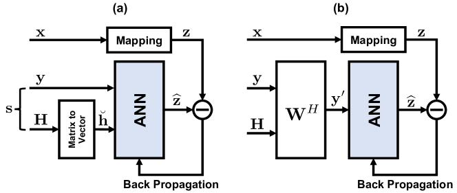
Figure 1: ANN-assisted coherent MIMO detection: (a) the ANN input is a combination of received signal and CSI; (b) the ANN input is a linearly filtered received signal.

Despite an increasingly hot topic, there is an ongoing debate on the use of machine learning for communication systems design, particularly on the modem side [8]. A straightforward question would be: modem based on the simple linear model (1) can be well optimized by hand-engineered means; what are additional values machine learning could bring to us; and what will be the cost? Basically, it is not our aim to join the debate with this paper. However, we find it useful to highlight a number of the key features of the ANN-assisted MIMO detection based on published results, as they well motivated our work. Specifically, ANN-assisted MIMO detection has the following remarkable advantages:

I-1 Parallel computing ready

ANN-assisted MIMO receivers are mostly based upon feed-forward neural networks, which have a parallel computing architecture in nature [9]. It fits into the trend of high-performance computing technologies that highly rely on parallel processing power to improve the computing speed, the capacity of multi-task execution as well as the computing energy-efficiency. This is an important feature as it equips the receiver with a great potential of providing ultra-low latency and energy-efficient signal processing that is one of key requirements for future wireless networks [10, 11].

I-2 Low receiver complexity

ANN-assisted MIMO receivers only involve a number of matrix multiplications, depending on the number of hidden layers involved in the feed-forward procedure. Moreover, they bypass channel matrix inversions or factorizations (such as singular-value decomposition or QR decomposition) which are needed for most of conventional MIMO receivers including linear ZF, LMMSE [12], successive interference cancellation (SIC) [13], sphere decoding [14], and many others [15]. The complexity for channel matrix inversions or factorizations is around $\mathcal{O}(NM^{2})$ with $(N\geq M)$. This can be affordable complexity for current real-time digital signal processing (DSP) technology as long as the size of the channel matrix is reasonably small (e.g. $M=10$ or smaller) [16]. However, such rather prevents the development of future MIMO technologies that aim to exploit increasingly the spatial degree of freedom for spectral efficiency. One might argue for the use of high-performance parallel computing technologies to mitigate this bottleneck. However, there is a lack of parallel computing algorithms for matrix inversions or something equivalent to this date.

I-3 Good performance-complexity trade-off

it has been demonstrated that extensively trained ANN-assisted receivers can be well optimized for their training environments (or channel models). For instance in [17], the performance of ANN-assisted receiver is very close to that of the MLSD. This is rather encouraging result as it reaches a good trade-off between the receiver complexity and the performance.

Despite their advantages, current ANN-assisted MIMO receivers face a number of fundamental challenges.

I-1 ANN learning scalability

in MIMO fading channels, the ANN blackbox in Fig. 1-(a) has its learning capacity rapidly degraded with the growth of transmit antennas [18]. Current approaches to mitigate this problem are by means of training the ANN with channel equalized signals; as depicted in Fig. 1-(b). However, in this case, ANN-assisted receivers are not able to exploit maximally the spatial diversity-gain due to the multiuser orthogonalization enabled by channel equalizers [19], and as a consequence, their performances go far away from the MLSD receiver.

I-2 Learning expenses

the ANN learning process often involves very expensive computation cost and energy consumption as far as the conventional computing architecture is concerned. The aim of reducing ANN learning expenses has recently motivated a new research area on non von Neumann computing architectures [20].

I-3 Training set over-fitting

an ANN-assisted receiver trained for a specific wireless environment (or channel model) is often not suitable for another environment (or channel model) [21]. This issue can be viewed more positively. For instance in urban areas, access points (AP), such as LTE eNBs or 5G gNBs, often have their physical functions optimized for local environments [22]. It could be an advantage if MIMO transceivers integrated in APs can also be optimized for their local environments through machine learning.

I-4 The black-box problem

it is well recognized that the black-box model is challenging the system reliability and maintenance job. “How to make artificial intelligence (AI) more describable or explainable?” becomes an increasingly important research topic in the general AI domain [23, 24, 25].

Again, we stress that the objective of this paper is not to offer a comparison between machine learning and hand-engineered approaches in the scope of MIMO detection. Instead, our aim is to develop a deeper understanding of the fundamental behaviors of ANN-assisted MIMO detection, based on which we can find a scalable approach for that. Major contributions of this paper include:

• An extensive study of the ANN-assisted MIMO detection model in terms of its performance and scalability. By borrowing the basic concept from the ANN vector quantization (VQ) model used for source encoding in [26], our work reveals that ANN-assisted MIMO detection can be modeled as the ANN-assisted lossy VQ, named MIMO-VQ, which is naturally a joint statistical channel quantization and massage quantization procedure. By means of the nearest-neighbor (NN) mapping, MIMO-VQ is shown to be integer least-squares optimum with its complexity growing exponentially with the number of transmit antennas;

• The analysis of codebook-vector combination approaches including cluster-level nearest neighbor (CL-NN) and cluster-level kNN (CL-kNN). It is shown that both approaches require much less neurons than the NN-based MIMO-VQ. However, those low-complexity approaches introduce considerable loss to the statistical channel quantization (equivalently increase of channel ambiguity for the message quantization), which results in learning inefficiency particularly at higher signal-to-noise ratios (SNR);

• The development of MNNet, a novel modular neural network (MNN) based MIMO detection approach that can achieve near-optimal performance with much lower computational complexity than state-of-the-art deep-learning based MIMO detection methods. The idea of MNNet lies in the integration of parallel interference cancellation (PIC)in deep MNN, which linearly reduces the interference (or equivalently the number of transmit-antennas) along the feed-forward propagation; and so as the quantization loss. Moreover, the learning procedure of MNNet can be applied at the modular level; and this largely reduces the learning complexity.

The rest of this paper is organized as follows. Section II presents the novel ANN-assisted MIMO-VQ model. Section III presents fundamental behaviors of the ANN-assisted MIMO-VQ as well as the learning scalability. Section IV presents the novel MNNet approach as well as the performance and complexity analysis. Simulation results are presented in Section V; and finally, Section VI draws the conclusion.

II MIMO-VQ Model for The ANN-Assisted MIMO Detection

II-A Concept of Vector Quantization

A vector quantizer is a statistical source encoder, which aims to efficiently and compactly represent the original signal using a digital signal. The encoded signal shall retain the essential information contained in the original signal [27]. More rigorously, VQ can be described by

Definition 1 ([26])

Given an arbitrary input vector $\mathbf{s}\in\mathbb{R}^{K\times 1}$ and a finite set $\mbox{\boldmath$\mathcal{A}$}=\{0,1,...,J-1\}$, VQ forms a mapping: $\mathbf{s}\longrightarrow j$, with $j\in\mbox{\boldmath$\mathcal{A}$}$ denoting the index of codebook vectors. Given $p_{j}$ the probability when $\mathbf{s}$ is mapped to $j$, the average rate of the codebook vectors is $R=-\sum_{j=0}^{J-1}p_{j}\log_{2}p_{j}$. Since each input vector has $K$ components, the number of bits required to encode each input vector component is $(R)/(K)$. Moreover, the compression rate of VQ is: $r=(R)/\hbar(\mathbf{s})$, where $\hbar(\mathbf{s})$ is the entropy of $\mathbf{s}$.

The aim of VQ is to find the optimum codebook which minimizes the average quantization loss (distortion) given the codebook size $J$.

Definition 2

Given $\hat{\mathbf{s}}_{j}\in\mathbb{R}^{K\times 1}$ the reconstructed input vector (or called the anchor vector) corresponding to $j$, and $\Delta(\mathbf{s},\hat{\mathbf{s}}_{j})$ the quantization loss when $\mathbf{s}$ is mapped to $j$, the average quantization loss is

$$\overline{\Delta}=\underset{\mathbf{s}}{\mathbb{E}}\left(\sum_{j=0}^{J-1}p_{j}\min_{j}\Delta(\mathbf{s},\hat{\mathbf{s}}_{j})\right)$$ (2)

where $\underset{\mathbf{s}}{\mathbb{E}}(\cdot)$ denotes the expectation over $\mathbf{s}$.

By means of minimizing the average quantization loss (2), VQ effectively partitions input vectors into $J$ clusters, and forms anchor vectors $\hat{\mathbf{s}}_{j},\forall j$; such is called the Voronoi partition.

II-B ANN-Assisted Vector Quantization

ANN architecture for VQ is rather straightforward. Consider a neural network having $J$ neurons, with each yielding a binary output $\hat{z}_{j}\in\{0,1\}$. Let $\mathbf{w}_{j}$ be the weighting vector for the $j^{\text{th}}$ neuron. ANN can measure the quantization loss $\Delta(\mathbf{s},\mathbf{w}_{j})$ and apply the NN rule to determine the output $\hat{z}_{j}$, i.e.,

$$\hat{z}_{j}=\left\{\begin{array}[]{cl}1,&\Delta(\mathbf{s},\mathbf{w}_{j})=\min\Delta(\mathbf{s},\mathbf{w}_{l}),l=0,...,J-1\\ 0,&\text{otherwise}\end{array}\right.$$ (3)

Right after the ANN training, we let $\hat{\mathbf{s}}_{j}=\mathbf{w}_{j}$. Such shows how input vectors are optimally partitioned into $J$ clusters.

The ANN training procedure often starts with a random initialization for the weighting vectors $\mathbf{w}_{j},\forall j$. Then, the training algorithm iteratively adjusts the weighting vectors with

$$\mathbf{w}_{j}(i+1)=\mathbf{w}_{j}(i)+\beta(i)(\mathbf{s}-\mathbf{w}_{j}(i))z_{j}(i)$$ (4)

where $i$ denotes the number of iterations, and $\beta(i)$ is the adaptive learning rate, which typically decreases with the growth of iterations. This is the classical Hebbian learning rule for the competitive unsupervised learning [28], which has led to a number of enhanced or extended versions such as the Kohonen self-organizing feature map algorithm [29], learning VQ [30], and frequency selective competitive learning algorithm [31]. Nevertheless, all of those unsupervised learning algorithms go beyond the scope of our research problem, and thus we skip the detailed discussion in this paper.

II-C ANN-Assisted MIMO Vector Quantization

Let us form an input vector $\mathbf{s}=[\breve{\mathbf{h}}^{T},\mathbf{y}^{T}]^{T}$, where $\mathbf{y}$ is the received signal vector; $\breve{\mathbf{h}}$ is the CSI vector as already defined in Section I; and $[\cdot]^{T}$ stands for the matrix or vector transpose. All notations are now redefined in the real domain, i.e., $\mathbf{y}\in\mathbb{R}^{N\times 1}$, $\mathbf{H}\in\mathbb{R}^{N\times M}$, $\mathbf{x}\in\mathbb{R}^{M\times 1}$. Since $\breve{\mathbf{h}}$ is the vector counterpart of $\mathbf{H}$, the length of $\breve{\mathbf{h}}$ is $(NM)$, and consequently the length of $\mathbf{s}$ is: $K=N(M+1)$. Note that the conversion from complex signals to their real-signal equivalent version doubles the size of corresponding vectors or matrices [32] (can be also found in Section IV). However, we do not use the doubled size for the sake of mathematical notation simplicity.

Furthermore, we form a finite set $\mathcal{A}$ with the size $J=L^{M}$. Every element in $\mathcal{A}$ forms a bijection to their corresponding codebook vector $\mathbf{x}_{j}\in\mathbb{R}^{M\times 1}$. According to Definition 1, VQ can be employed to form the mapping: $\mathbf{s}\longrightarrow j\longrightarrow\hat{\mathbf{x}}_{j}$. For the MIMO detection, $\hat{\mathbf{x}}$ is the reconstructed version of $\mathbf{x}$, and thus it should follow the same distribution as $\mathbf{x}$ (i.e. the equal probability). Then, the average rate of codebook vectors becomes $R=M\log_{2}L$; and the compression rate of VQ is

$$r=\frac{M\log_{2}L}{\hbar(\mathbf{s})}$$ (5)

The average quantization loss given in Definition 2 becomes

$$\overline{\Delta}=\frac{1}{J}\sum_{j=0}^{J-1}\underset{\mathbf{s}}{\mathbb{E}}\Big{(}\min_{j}\Delta(\mathbf{s},\hat{\mathbf{s}}_{j})\Big{)}$$ (6)

Theoretically, the ANN architecture introduced in Section II-B can be straightforwardly employed for the MIMO-VQ. By means of the NN mapping, there will be $\bar{J}=L^{M}$ neurons integrated in the ANN, with each employing a binary output function. This might cause the well-known curse of dimensionality problem since neurons required to form the ANN grow exponentially with the number of transmit antennas and polynomially with the modulation order. For instance, there is a need of $\bar{J}=16^{4}$ neurons to detect MIMO signals sent by $M=4$ transmit antennas, with each modulated by $16$-QAM; and this is surely not a scalable solution.

A considerable way to scale up the ANN-assisted MIMO-VQ is to employ the k-nearest neighbor (kNN) rule (see [33]) to determine the output $\hat{z}_{j}$ , i.e.,

$$\hat{z}_{j}=\left\{\begin{array}[]{cl}1,&\Delta(\mathbf{s},\mathbf{w}_{j})\in\{\text{k-min}\Delta(\mathbf{s},\mathbf{w}_{l}),\forall l\}\\ 0,&\text{otherwise}\end{array}\right.$$ (7)

where $\text{k-min}(\cdot)$ stands for the function to obtain the K minimums in a set. By such means, we can have $J\choose{\text{K}}$ codebook vectors through a combination of $\mathbf{w}_{j},\forall j$. It is possible to further scale up MIMO-VQ through kNN with $\text{k}=1,...,K$, by means of which we have the capacity to form $\sum_{\text{k}=1}^{\text{K}}{J\choose{\text{k}}}$ codebook vectors [34].

Unlike conventional VQ techniques, MIMO-VQ can be associated with the supervised learning [18]. At the training stage, the ANN exactly knows the mapping: $\mathbf{s}\longrightarrow j$, and thus it can iteratively adapt $\mathbf{w}_{j}$ to minimize the distortion $\Delta(\mathbf{s},\mathbf{w}_{j})$; and such largely reduces the learning complexity. Moreover, the knowledge of mapping $\mathbf{s}\longrightarrow j$ facilitates the combination of codebook vectors by which the number of required neurons can be significantly reduced. Currently, there are two approaches for the codebook-vector combination:

II-C1 Cluster-level nearest neighbor

consider an ANN consisting of $\bar{J}=ML$ neurons. Neurons are divided into $M$ clusters indexed by $m$, corresponding to the $m^{\mathrm{th}}$ element in $\mathbf{x}$. Each cluster has $L$ neurons indexed by $l$, corresponding to the $l^{\mathrm{th}}$ state of an element in $\mathbf{x}$. VQ forms a mapping $\mathbf{s}\longrightarrow(l_{1},...,l_{M})$, with $l_{m}$ denoting the $l^{\text{th}}$ neuron within the $m^{\text{th}}$ cluster. The output is now indexed by $\hat{z}_{l,m}$, which is determined by the CL-NN rule, $\forall m$

$$\hat{z}_{l,m}=\left\{\begin{array}[]{cl}1,&\Delta(\mathbf{s},\mathbf{w}_{l,m})=\min\Delta(\mathbf{s},\mathbf{w}_{\ell,m}),\forall\ell\\ 0,&\text{otherwise}\end{array}\right.$$ (8)

By such means, one can use $(LM)$ neurons to represent $L^{M}$ codebook vectors.

II-C2 Cluster-level kNN

consider an ANN consisting of $\bar{J}=M\log_{2}L$ neurons. Again, we can divide neurons into $M$ clusters. Each cluster now has $\alpha(=\log_{2}L)$ neurons. VQ maps $\mathbf{s}$ to the corresponding output $\hat{z}_{l,m}$ through the CL-kNN rule

$$\hat{z}_{l,m}=\left\{\begin{array}[]{cl}1,&\Delta(\mathbf{s},\mathbf{w}_{l,m})\in\text{k-min}\Delta(\mathbf{s},\mathbf{w}_{\ell,m}),\forall\ell\\ 0,&\text{otherwise}\end{array}\right.$$ (9)

with $\text{k}\in\{1,...,L\}$. By such means, one can use $M\log_{2}L$ neurons to represent $L^{M}$ codebook vectors.

It is worth noting that both CL-NN and CL-kNN are more suitable for supervised learning than unsupervised learning as far as the learning complexity is concerned. The ideas themselves are not novel. However, it is the first time in the literature that uses the VQ model to mathematically describe the ANN-assisted MIMO detection; and they lay the foundation for further investigations in other sections.

III Fundamental Behaviors of MIMO Vector Quantization

The VQ concept presented in Section II equips us with sufficient basis to develop a deeper understanding on fundamental behaviors of the ANN-assisted MIMO-VQ.

III-A MIMO-VQ Compression Behavior

In applications such as image, video, or speech compression, VQ has a controllable compression rate or quantization loss by managing the codebook size [35, 36]. However, this is not the case for MIMO-VQ, as the codebook size is determined by the original signal.

Theorem 1

Assuming the MIMO channel matrix $\mathbf{H}$ to be i.i.d., the compression rate of MIMO-VQ decreases linearly or more with the number of transmit antennas $M$. Moreover, we have $\lim_{M\rightarrow\infty}r=0$.

Proof:

Given the i.i.d. MIMO channel, we will have $\hbar(\breve{\mathbf{h}})=\sum_{n=0}^{N-1}\sum_{m=0}^{M-1}\hbar(H_{nm})=MN\sigma_{H}^{2}$, where $H_{nm}$ denotes the $(n,m)^{\text{th}}$ entry of $\mathbf{H}$ that has the entropy $\sigma_{H}^{2}$. The entropy of $\mathbf{s}$ is

$$\hbar(\mathbf{s}) =\hbar(\mathbf{y})+\hbar(\mathbf{H})$$ (10)

$$\geq\hbar(\mathbf{x}|\mathbf{H})+\hbar(\mathbf{H})$$ (11)

$$\geq\hbar(\mathbf{x})+\hbar(\mathbf{H})$$ (12)

$$\geq M(\sigma_{x}^{2}+N\sigma_{H}^{2})$$ (13)

The equality in (11) holds in the noiseless case, and $\hbar(\mathbf{x}|\mathbf{H})=\hbar(\mathbf{x})$ due to $\mathbf{x}$ being independent from $\mathbf{H}$ in communication systems. The information compression rate is therefore given by

$$r=\frac{\hbar(\mathbf{x})}{\hbar(\mathbf{s})} \leq\frac{\sigma_{x}^{2}}{\sigma_{x}^{2}+N\sigma_{H}^{2}}$$ (14)

$$\leq(1+M(\sigma_{H}^{2})/(\sigma_{x}^{2}))^{-1}$$ (15)

We can also use the VQ compression rate (5) to obtain

$$r\leq(1+M(\sigma_{H}^{2})/(\log_{2}L))^{-1}$$ (16)

as far as the quantization of $\mathbf{x}$ is concerned. Both (15) and (16) show that the upper bound of the compression rate decreases linearly with $M$. For $M\rightarrow\infty$, it is trivial to justify that the upper bound tends to zero. Theorem 1 is therefore proved. ∎

The information-theoretical result in Theorem 1 implies that MIMO-VQ introduces the rate distortion $(1-r)$, which grows at least linearly with $M$. Moreover, the rate distortion approaches $100\%$ due to $\lim_{M\rightarrow\infty}r=0$; and such challenges the scalability of MIMO-VQ.

III-B MIMO-VQ Quantization Behavior

We use the nearest-neighbor rule (3) to study the MIMO-VQ quantization behavior, appreciating its optimality as well as the simple mathematical form. Our analysis starts from the following hypothesis:

Proposition 1

Split the reconstructed vector $\hat{\mathbf{s}}_{j}$ into two parts: $\hat{\mathbf{s}}_{j}=[(\hat{\mathbf{s}}_{j}^{(1)})^{T},(\hat{\mathbf{s}}_{j}^{(2)})^{T}]^{T}$, with $\hat{\mathbf{s}}_{j}^{(1)}\in\mathbb{R}^{N\times 1}$, $\hat{\mathbf{s}}_{j}^{(2)}\in\mathbb{R}^{(MN)\times 1}$. The quantization loss $\Delta(\mathbf{s},\hat{\mathbf{s}}_{j})$ can be decoupled into

$$\Delta(\mathbf{s},\hat{\mathbf{s}}_{j})=\Delta(\mathbf{y},\hat{\mathbf{s}}_{j}^{(1)})+\Delta(\breve{\mathbf{h}},\hat{\mathbf{s}}_{j}^{(2)})$$ (17)

Proposition 1 is true when we use the squared Euclidean-norm to measure the quantization loss; and in this case, VQ is least-squares optimal.

After training, the nearest-neighbor rule effectively leads to the forming of $J$ spheres, with each having their center at $\hat{\mathbf{s}}_{j}$ and radius $d_{j}$, i.e.,

$$\Delta(\mathbf{s},\hat{\mathbf{s}}_{j})\leq d_{j},\forall j.$$ (18)

Moreover, we shall have

$$\Delta(\mathbf{y},\hat{\mathbf{s}}_{j}^{(1)})\leq d_{j}^{(1)}$$ (19)

$$\Delta(\breve{\mathbf{h}},\hat{\mathbf{s}}_{j}^{(2)})\leq d_{j}^{(2)}$$ (20)

It is possible for $\mathbf{s}$ to fall into more than one sphere as described in (18). In the ANN implementation, this problem can be solved through the use of softmax activation function [18]. It is therefore reasonable to assume that $\mathbf{s}$ will only fall into one of the spheres. The MIMO detection will have errors when

$$\Delta(\mathbf{s},\hat{\mathbf{s}}_{j})\leq d_{j},~{}\text{for}~{}\mathbf{s}\longrightarrow\mathbf{x}_{i}\longrightarrow\hat{\mathbf{s}}_{i},i\neq j$$ (21)

In order to prevent this case from happening in the noiseless context, we shall have the following condition.

Theorem 2

Assuming: a1) $\mathbf{H}_{j}\mathbf{x}_{j}=\mathbf{H}_{i}\mathbf{x}_{i}$, $\forall i\neq j$, a sufficient condition to prevent (21) from happening in the noiseless context is

$$\Delta(\breve{\mathbf{h}}_{i},\hat{\mathbf{s}}_{j}^{(2)}) \geq d_{j}^{(2)}$$ (22)

$$\Delta(\mathbf{H}_{i}\mathbf{x}_{j},\hat{\mathbf{s}}_{j}^{(1)}) <d_{j}-d_{j}^{(2)}$$ (23)

Proof:

In the noiseless case, given the channel realization $\mathbf{H}_{j}$, (17) can be written into

$$\Delta(\mathbf{s}_{j},\hat{\mathbf{s}}_{j})=\Delta(\mathbf{H}_{j}\mathbf{x}_{j},\hat{\mathbf{s}}_{j}^{(1)})+\Delta(\breve{\mathbf{h}}_{j},\hat{\mathbf{s}}_{j}^{(2)})\leq d_{j}$$ (24)

Considering $\mathbf{s}_{i}\longrightarrow\mathbf{x}_{i}$ with the channel realization $\mathbf{H}_{i}$, we have the quantization loss

$$\Delta(\mathbf{s}_{i},\hat{\mathbf{s}}_{j})=\Delta(\mathbf{H}_{i}\mathbf{x}_{i},\hat{\mathbf{s}}_{j}^{(1)})+\Delta(\breve{\mathbf{h}}_{i},\hat{\mathbf{s}}_{j}^{(2)})>d_{j}$$ (25)

Given the assumption a1), (25) becomes

$$\Delta(\mathbf{s}_{i},\hat{\mathbf{s}}_{j})=\Delta(\mathbf{H}_{j}\mathbf{x}_{j},\hat{\mathbf{s}}_{j}^{(1)})+\Delta(\breve{\mathbf{h}}_{i},\hat{\mathbf{s}}_{j}^{(2)})>d_{j}$$ (26)

To simultaneously fulfill (24) and (26) leads to

$$\Delta(\breve{\mathbf{h}}_{j},\hat{\mathbf{s}}_{j}^{(2)})\leq d_{j}-\Delta(\mathbf{H}_{j}\mathbf{x}_{j},\hat{\mathbf{s}}_{j}^{(1)})<\Delta(\breve{\mathbf{h}}_{i},\hat{\mathbf{s}}_{j}^{(2)}),\forall i\neq j$$ (27)

(27) should hold for all possible realizations of $\mathbf{H}_{j}$ (or $\breve{\mathbf{h}}_{j}$). This condition can be guaranteed by replacing $\Delta(\breve{\mathbf{h}}_{j},\hat{\mathbf{s}}_{j}^{(2)})$ with the upper bound (20); and such leads to (22).

Furthermore, $\mathbf{H}_{i}$ can also be a possible realization of $\mathbf{H}_{j}$. In this case, we have

$$\Delta(\mathbf{s}_{j},\hat{\mathbf{s}}_{j})=\Delta(\mathbf{H}_{i}\mathbf{x}_{j},\hat{\mathbf{s}}_{j}^{(1)})+\Delta(\breve{\mathbf{h}}_{i},\hat{\mathbf{s}}_{j}^{(2)})\leq d_{j}$$ (28)

Applying the second inequality of (27) into (28) yeilds

$$\Delta(\mathbf{H}_{i}\mathbf{x}_{j},\hat{\mathbf{s}}_{j}^{(1)}) <\Delta(\mathbf{H}_{j}\mathbf{x}_{j},\hat{\mathbf{s}}_{j}^{(1)})$$ (29)

$$<d_{j}-\Delta(\breve{\mathbf{h}}_{j},\hat{\mathbf{s}}_{j}^{(2)})$$ (30)

To guarantee the inequality (30), $\forall j$, we shall replace $\Delta(\breve{\mathbf{h}}_{j},\hat{\mathbf{s}}_{j}^{(2)})$ with their maximum $d_{j}^{(2)}$. The result (23) is therefore proved. ∎

Theorem 2 indicates that MIMO-VQ actually consists of two parts of quantization, i.e., one for the CSI quantization, and the other for the received signal quantization. For the CSI quantization, each neuron statistically partitions CSI realizations into different groups according to the rule $\Delta(\breve{\mathbf{h}},\hat{\mathbf{s}}_{j}^{(2)})\gtreqless d_{j}^{(2)}$, where the threshold $d_{j}^{(2)}$ is determined through supervised learning. Theoretically, the use of $\bar{J}$ neurons can result in $2^{\bar{J}}$ different CSI groups as a maximum. However, a channel realization fulfilling $\Delta(\breve{\mathbf{h}},\hat{\mathbf{s}}_{j}^{(2)})\geq d_{j}^{(2)}$ does not normally fulfill $\Delta(\breve{\mathbf{h}},\hat{\mathbf{s}}_{i}^{(2)})\geq d_{i}^{(2)},\forall i\neq j$; and thus, CSI realizations will only be partitioned into $\bar{J}$ groups, with each corresponding to a state for the transmitted signal partition. Thus, CSI quantization loss is inevitable when the number of channel realization sample is larger than the number of neurons on the output layer. As a result, an error floor is expected to occur at high SNR regime because of the learning inefficiency, i.e., channel ambiguity. More intuitively, the MIMO-VQ principle is illustrated in Fig. 2,

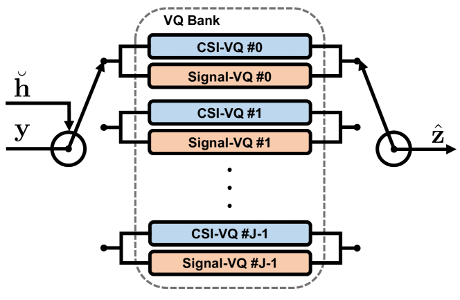
Figure 2: Illustration of the MIMO-VQ principle.

where the channel realization, $\breve{\mathbf{h}}$, together with received signal, $\mathbf{y}$, are mapped onto one out of the $\bar{J}$ states. It is worth noting that CSI quantization aims to remove the channel ambiguity defined in Definition 2. Meanwhile, the signal VQ performs a mapping $\mathbf{y}\longrightarrow\hat{\mathbf{z}}$, where $\mathbf{z}$ is the supervisory training target as described in (7).

The major bottleneck here is again the Curse of Dimensionality problem [37], as CSI realizations are classified into $\bar{J}$ states which grow exponentially with the number of data streams $M$. When either CL-NN or CL-kNN (see Section II-C) is employed for the VQ, $\bar{J}$ grows linearly with $M$. However, such reduces the resolution of channel quantization and consequently increases the channel ambiguity in signal detection.

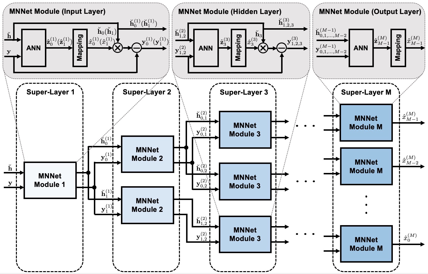
Figure 3: Block diagram of the proposed MNNet.

III-C Channel-Equalized Vector Quantization

Section III-B shows that channel quantization scales down the ANN-assisted MIMO detectability. This straightforwardly motivates the channel-equalized VQ model as depicted in Fig. 1-(b). When channel equalizers (such as ZF and LMMSE) are employed, MIMO-VQ simply serves as a symbol de-mapper in Gaussian noise; and thus, there is no channel quantization loss. On the other hand, channel equalizers often require channel matrix inversion, which is of cubic complexity and not ready for parallel computing. More critically, the ANN-assisted receiver cannot achieve the MLSD performance as shown in [18], and there is lacking convincing advantages of using machine learning for the MIMO detection. The only exceptional case is to use the MF for the channel equalization, which supports parallel computing and low complexity. It is shown in [18] that MIMO-VQ is able to improve the MF detection performance by exploiting the sequence-detection gain. This is because the MF channel equalizer does not remove the antenna correlation as much as the ZF and LMMSE algorithms, and leaves room for the ANN to exploit the residual sequence detection gain. On the other hand, the MF-ANN approach has its performance far away from the MLSD approach. Detailed computer simulation is provided in Section V.

IV The MNNet Approach for MIMO-VQ

In this section, we introduce a novel MNN-based deep learning approach, named MNNet, which combines modular neural network [38] with PIC algorithm [39].

IV-A MNNet Architecture

The structure of the proposed MNNet is illustrated in Fig. 3. The entire network consists of $M$ cascade super-layers, and each layer has a similar structure that contains a group of MNNet modules instead of neurons. The MNNet modules on the same super-layer are identical, and those on different super-layers function differently. Besides, the MNNet modules on the front $M-1$ super-layers share similar structures, which consist of three basic components: An ANN, a codebook mapping function and an interference cancellation unit. The $M^{\mathrm{th}}$ super-layer does not have the interference cancellation unit because the output of its mapping function is the information-bearing symbols.

The input to the first super-layer is a concatenation of the CSI vector $\breve{\mathbf{h}}$ and the received signal vector $\mathbf{y}$. It is perhaps worth noting that communication signals are normally considered as complex-valued symbols, but most of the existing deep learning algorithms are based on real-valued operations. To facilitate the learning and communication procedure, it is usual practice to convert complex signals to their real signal equivalent version using (31) (see [5, 6, 7, 17, 32]). For instance, a $(K)\times(1)$ complex-valued input vector $\mathbf{s}$ is converted into a $(2K)\times(1)$ real-valued vector $\mathbf{s}_{\text{real}}$ by concatenating its real and imaginary parts, which is given by

$$\mathbf{s}_{\text{real}}=\begin{bmatrix}~{}\Re(\mathbf{s})~{}\\ ~{}\Im(\mathbf{s})~{}\end{bmatrix}$$ (31)

The output of ANN is the estimate of entire codebook vector $\hat{\mathbf{z}}^{(1)}$ as we introduced in Section II-B&C, where the superscript $[\cdot]^{(1)}$ stands for the number of super-layer. In order to simplify the network structure, only the first two transmitted symbols $\hat{x}_{0}^{(1)}(\hat{x}_{1}^{(1)})$ are mapped back from the estimated codebook vector $\hat{\mathbf{z}}_{0}^{(1)}(\hat{\mathbf{z}}_{1}^{(1)})$ by applying the pre-defined bijection mapping functions (e.g. NN, CL-NN or CL-kNN). Denote $\breve{\mathbf{h}}_{m}$ to the channel coefficients between the $m^{\mathrm{th}}$ transmit antenna to the MIMO receiver, the interference cancellation procedure can be described as

$$\mathbf{y}_{m}^{(1)}=\mathbf{y}-\breve{\mathbf{h}}_{m}\hat{x}_{m}^{(1)},~{}_{m\in\left\{0,1\right\}}$$ (32)

which, together with part of the CSI vector $\breve{\mathbf{h}}_{m}^{(1)}$ serves as the input to the second super-layer, i.e., $\mathbf{s}_{m}^{(1)}=[\mathbf{y}_{m}^{(1)T},\breve{\mathbf{h}}_{m}^{(1)T}]^{T},~{}_{m\in\left\{0,1\right\}}$, where $\breve{\mathbf{h}}_{m}^{(1)}$ is obtained by removing $\breve{\mathbf{h}}_{m}$ from $\breve{\mathbf{h}}$. Therefore, the second super-layer will consist of two parallel MNNet modules where the outputs from the previous super-layer are processed separately. In order to obtain an estimate of every transmitted symbol $\hat{x}_{m},~{}_{0\leq m\leq M-1}$, the top branch on each super-layer needs to produce two outputs as depicted in Fig. 3. Furthermore, the MNNet modules on the front $M-1$ super-layers share similar structure except for the size of ANN input and output. Specifically, the size of input to the $m^{\mathrm{th}}$ super-layer is $2N(M-m+2)$, and output is $2^{(M-m+1)\cdot\log_{2}L}$ when NN mapping rule is considered. By repeating this process for $M$ times, the output of the $M^{\mathrm{th}}$ super-layer are the final estimates of transmitted symbols.

IV-B Scalability and Computational Complexity

The information-theoretical result in (15) and (16) implies that ANN-assisted MIMO-VQ introduces the rate distortion, which grows at least linearly with the number of transmit antennas $M$. The proposed MNNet scales up the MIMO-VQ solution by reducing the number of data streams on a layer-by-layer basis. The upper bound of the compression rate increases along the feed-forward propagation. On the other hand, MNNet involves a large number of modules.

Proposition 2

Concerning every super layer to be associated with the PIC algorithm, the MNNet involves in total $M(M+1)/2$ modules to conduct the MIMO signal detection.

Proof:

As shown in Fig. 3, there are $M$ super layers forming the MNNet. On each $m^{\mathrm{th}}$ super layer ($m=1,...,M$), MNNet module eliminates $(m-1)$ interferences, and then perform the VQ procedure. According to the PIC principle, interferences eliminated at MNNet modules have to be different and in order. Hence, the $m^{\mathrm{th}}$ super layer needs $P(M,m-1)$ modules, where $P(,)$ denotes the permutation. However, since every transmitted symbol are independently drawn from a finite-alphabet set with equal probability. It is trivial to justify that the average error probability of each reconstructed transmitted symbol is equal. Therefore, the total number of modules employed in MNNet can calculated by

$$\mathcal{Q}(M) =\sum_{m=1}^{M}m$$ (33)

$$=M(M+1)/2$$

Proposition 2 is therefore proved. ∎

Since the MNNet is well modularized, the learning procedure does not need to be applied on the entire network as a whole, but rather at the modular level. Such a strategy largely improves the computational efficiency at the ANN training stage. The computational complexity required for MNNet training per module per iteration is approximately $\mathcal{O}(bNM)$, where $b$ is the size of mini-batch; and $\mathcal{O}(NM^{2})$ per detection. To put this in perspective, DetNet has a complexity of $\mathcal{O}(dN^{2})$, where $d$ is the number of iterative layers. OAMPNet has a higher complexity of $\mathcal{O}(dN^{3})$ dominated by the matrix inversion. The LMMSE algorithm similarly requires a matrix inversion, resulting in a complexity of $\mathcal{O}(N^{3})$.

V Simulation Results and Analysis

This section presents the experimental results and related analysis. The data sets and experimental setting are introduced at the beginning, followed by a brief introduction of the competing algorithms. After that, a comprehensive performance evaluation is given, which demonstrates the performance of the proposed MNNet approach.

V-A Data Sets and Experimental Setting

In traditional deep learning applications such as image processing and speech recognition, the performance of different algorithms and models are evaluated under common benchmarks and open data sets (e.g. MNIST, LSUN) [40]. It is a different story in wireless communication domain since we are dealing with artificially manufactured data that can be accurately generated. Therefore, we would like to define the data generation routines instead of giving specific data sets.

As far as the supervised learning is concerned, every training sample is a mainstay containing an input object and a supervisory output. According to the system model in (1), the transmitted signal $\mathbf{x}$ is an $(M)\times(1)$ vector with each symbol drawn from a finite-alphabet set $\mathcal{A}$ consisting of $L$ elements. There are a total number of $J=L^{M}$ possible combinations, and $\mathbf{x}_{j}$ denotes the $j^{\text{th}}$ combination. By applying the NN rule, the corresponding supervisory representation of $\mathbf{x}_{j}$ can be expressed by

$$\mathbf{z}_{j}=[\mathbf{1}(\mathbf{x}_{j}=\mathbf{x}_{0}),\mathbf{1}(\mathbf{x}_{j}=\mathbf{x}_{1}),\cdots,\mathbf{1}(\mathbf{x}_{j}=\mathbf{x}_{J-1})]^{T}$$ (34)

where $\mathbf{1}(\cdot)$ is the indicator function. It is easy to find that $\mathbf{z}_{j}$ is a $(J)\times(1)$ one-hot vector with only one element equals to one and others are zero. Meanwhile, other codeword mapping approaches including CL-NN and CL-kNN can be implemented through similar method as described in (8) or (9). Due to the channel randomness, each transmitted signal can yield to multiple received signals even in the noiseless case. Denote $\mbox{\boldmath$\mathcal{B}$}_{j}$ to the feasible set which contains all possible received signal vectors when $\mathbf{x}_{j}$ is transmitted, $\mathbf{y}_{i,j}\in\mbox{\boldmath$\mathcal{B}$}_{j}$ to the $i^{\text{th}}$ element of $\mathcal{B}$ and $\breve{\mathbf{h}}_{i,j}$ to the corresponding channel realization. Then, the pairwise training sample can be described as

$$\left\{[\breve{\mathbf{h}}_{i,j}^{T},\mathbf{y}_{i,j}^{T}]^{T},\mathbf{z}_{j}\right\}$$ (35)

and the goal of neural network training is to minimize the following objective function

$$\varphi^{*}=\underset{\varphi}{\arg\min}~{}\mathcal{L}\left(\mathbf{z}_{j},\hat{\mathbf{z}}_{j}\right)$$ (36)

by adjusting the trainable parameters $\varphi=\left\{\mathbf{W},\mathbf{b}\right\}$, where $\mathcal{L}(\cdot)$ denotes to loss function, $\mathbf{W}$ and $\mathbf{b}$ to the weight and bias, and $\hat{\mathbf{z}}_{j}$ to the ANN reconstructed vector. The most popular method for updating parameters $\varphi$ is backpropagation together with stochastic gradient descent [41], which start with some randomly initialized values and iteratively converge to an optimum point. Furthermore, there are many adaptive learning algorithms which dramatically improve the convergence performance in neural network training procedure [42]. In this paper, AdaBound algorithm (see [43] for detailed description) is applied for performance evaluation

All the experiments are run on a Dell PowerEdge R730 2x 8-Core E5-2667v4 Server, and implemented in MATLAB.

V-B Baseline Algorithms for Performance Comparison

In our experiments, the following algorithms are employed for performance comparison:

• ZF: Linear detector that applies the channel pseudo-inverse to restore the signal [44].

• LMMSE: Linear detector that applies the SNR-regularized channel pseudo-inverse to restore the signal [45].

• MF: Linear detector that has the lowest computational complexity among all MIMO detectors [46].

• MLSD: The optimum detection algorithm that requires an exhaustive search.

• DetNet: A deep learning approach introduced in [5], which applies a deep unfolding approach that transforms a computationally intractable probabilistic model into a set of cascaded deep neural networks.

• OAMPNet: A deep learning approach introduced in [7], which incorporates deep learning into the orthogonal AMP algorithm.

• IW-SOAV: An iterative detection algorithm for massive overloaded MIMO system based on iterative weighted sum-of-absolute value optimization [47].

• TPG-Detector: A deep learning approach introduced in [6], which is designed specifically for massive overloaded MIMO system.

V-C Simulations and Performance Evaluation

Our computer simulations are structured into five experiments. In experiment 1, we investigate the performance of different codebook combination approaches. In experiment 2, the impact of the size of channel realization set on the detection performance of MIMO-VQ model is studied. In experiment 3 and 4, we evaluate the detection performance of both channel-equalized VQ model and MIMO-VQ model. In experiment 5, a comprehensive performance evaluation is provided for the proposed MNNet algorithm. The key metric utilized for performance evaluation is the average bit error rate (BER) over sufficient Monte-Carlo trails of block Rayleigh fading channels. The SNR is defined as the average received information bit-energy to noise ratio per receive antenna (i.e. $E_{b}/N_{0}$).

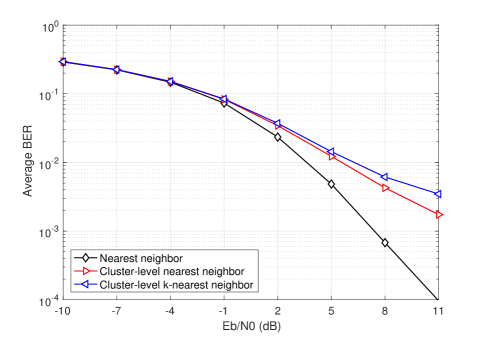
Figure 4: BER as a function of $E_{b}/N_{0}$ for MIMO-VQ model with different codebook combination approaches including NN, CL-NN and CL-kNN in uncoded 4-by-8 MIMO system with QPSK modulation.

TABLE I: Layout of the ANN

Layer	Output dimension
Input	$2K$
Dense + ReLU	$1024$
Dense + ReLU	$512$
Dense + ReLU	$256$
1) NN: Dense + softmax 2) CL-NN: Dense + cluster-level softmax 3) CL-kNN: Dense + sigmoid	1) $L^{M}$ 2) $ML$ 3) $M\log_{2}L$

Experiment 1

The aim of this experiment is to investigate the performance of different codebook combination approaches including NN, CL-NN and CL-kNN. The system environment is set to be an uncoded 4-by-8 MIMO network with QPSK modulation scheme. Moreover, Table I provides a detailed layout of ANN that applied for signal detection. The ANN training is operated at $E_{b}/N_{0}=5$ dB with a mini-batch size of 500; as the above configurations are found to provide the best detection performance.

Fig. 4 illustrates the average BER performance of the MIMO-VQ model with different codebook combination approaches. It is observed that NN significantly outperforms the other two approaches throughout the whole SNR range. For CL-NN, the detection performance decreased approximately 4.7 dB at BER of $10^{-3}$; and for CL-kNN, the gap is around 5 dB. The reason of performance degradation is because of the channel learning inefficiency, i.e., channel ambiguity. Moreover, CL-NN outperforms CL-kNN at high SNR range thanks to the use of more neurons on the output layer of ANN (i.e. $ML>M\log_{2}L$). The above phenomenons coincide with our conclusions made in Section II-B&C that NN offers the best performance among all codebook combination approaches. Both CL-NN and CL-kNN make a trade-off between computational complexity and performance. In order to demonstrate the best performance, NN is applied in the following experiments.

Experiment 2

The aim of this experiment is to investigate the impact of the size of channel realization set on the detection performance of MIMO-VQ model. The system environment and layout of ANN remain unchanged as we introduced in Experiment 1. Besides, the ANN is trained at $E_{b}/N_{0}=8$ dB with a mini-batch size of 500.

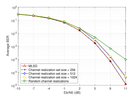
Figure 5: BER as a function of $E_{b}/N_{0}$ for MIMO-VQ model with different sizes of channel realization set in uncoded 4-by-8 MIMO system with QPSK modulation.

Fig. 5 illustrates the average BER performance of the MIMO-VQ model with different sizes of channel realization set. The channel data set is obtained by randomly generate a certain number of unique channel matrices and is utilized for both ANN training and testing phases. Since the environment is set to be an uncoded 4-by-8 MIMO with QPSK modulation, the number of neurons on ANN output layer is 256 (i.e. $\bar{J}=4^{4}$ as NN is considered). Therefore, we consider 4 different cases with the size of the channel realization set varies from 256 to infinite . The baseline for performance comparison is the optimum MLSD. It is observed that ANN-assisted MIMO receiver achieves optimum performance when the size of the set is 256, as the size of channel realizations matches the number of neurons on ANN output layer. By increasing the size to 512, the detection accuracy slightly degraded around 1 dB at high SNR range. Further increasing the size of channel realizations to 1024 does not make significant performance difference, as the gap between 512 and 1024 is almost negligible. The situation becomes different when the channel data set is not pre-defined (i.e. randomly generated every time). The average BER performance degraded about 2.5 dB at BER of $10^{-4}$. The above phenomenons coincide with our conclusion in Section III-B that channel quantization level bounds the signal quantization performance. When the size of the channel data set increases, the channel learning inefficient (i.e. channel ambiguity) causes the loss of detection accuracy particularly at high SNR range.

Experiment 3

This aim of this experiment is to demonstrate the performance of channel-equalized VQ model. Three commonly used channel equalizers are considered (e.g. ZF, LMMSE and MF). The layout of ANN is slight different since the input to ANN becomes the channel equalized signal block with a dimension of input equals to $2\times M$. Meanwhile, the output of ANN remains unchanged as introduced in Table I. Besides, the MIMO channel is considered as slow fading which varies every three transmission slots. The ANN is trained at $E_{b}/N_{0}=10$ dB with a mini-batch size of 500.

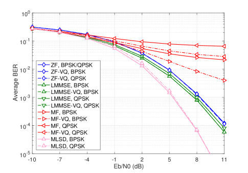
Figure 6: BER as a function of $E_{b}/N_{0}$ for channel-equalized VQ model in uncoded 4-by-8 MIMO system with BPSK/QPSK modulation.

Fig. 6 illustrates the average BER performance of channel-equalized VQ model in uncoded 4-by-8 MIMO system with both BPSK and QPSK modulation schemes. The baseline for performance comparison is the conventional channel equalizers. It is observed that ANN significantly improves the detection performance of MF equalizer at high SNR range. The deep learning gain is around 7 dB for BPSK and 10 dB for QPSK. This phenomenon indicates our conclusion in Section III-C that ANN is able to improve MF equalizer by exploiting more sequence detection gain. However, for both ZF and LMMSE equalizers, ANN does not offer any performance improvement, as the ANN serves as a simple additive white Gaussian noise (AWGN) de-mapper. Moreover, all of these approaches have their performances far away from the optimum MLSD in both BPSK and QPSK cases.

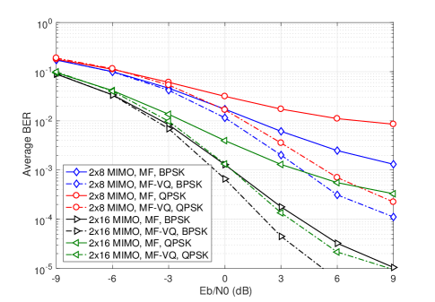
Figure 7: BER as a function of $E_{b}/N_{0}$ for MF-VQ model in uncoded MIMO system with BPSK/QPSK modulation.

Fig. 7 illustrates a more detailed performance evaluation for MF-VQ model. The performance of ANN is compared with the conventional MF equalizer. It is observed that MF-VQ model largely improves the detection performance in all scenarios. For 2-by-8 MIMO, the sequence detection gain is approximately 3 dB for BPSK and 5 dB for QPSK; and for 2-by-16 MIMO, the gain is more than 2 dB for BPSK and 4 dB for QPSK at high SNR range.

Experiment 4

The aim of this experiment is to demonstrate the performance of MIMO-VQ model with different modulation schemes. For BPSK and QPSK modulation, MIMO-VQ is trained at $E_{b}/N_{0}=5$ dB with a mini-batch size of 500; for 8-PSK and 16-QAM modulation, the training $E_{b}/N_{0}$ is set at 8 dB. The reason for training ANN at different SNR points for different modulation schemes is because we found different SNR points will result in different detection performances in ANN-assisted MIMO communications. Specifically, training at lower SNRs can obtain an ANN receiver only works well at low-SNR range, and vice versa. In order to achieve the best performance throughout the whole SNR range, we tested a few SNR points and the above settings are observed to achieve the best end-to-end performance among others.

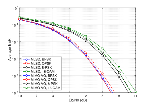
Figure 8: BER as a function of $E_{b}/N_{0}$ for MIMO-VQ model in uncoded 2-by-8 MIMO system with multiple modulation schemes.

Fig. 8 illustrates the average BER performance of MIMO-VQ model in uncoded 2-by-8 MIMO system with multiple modulation schemes. The baseline for performance comparison is the optimum MLSD. It is observed that MIMO-VQ model is able to achieve near-optimum performance in all cases. Specifically, the performance gap for BPSK is almost negligible; for QPSK and 8-PSK, the gap is around 0.8 dB at BER of $10^{-5}$; for 16-QAM, the gap increases to around 1.1 dB at BER of $10^{-5}$. Again, the performance gap is introduced by channel learning inefficient as we discussed in Experiment 2. Moreover, it is observed that channel quantization loss is more emergent for higher modulation schemes. This is perhaps due to the denser constellation points in higher-order modulation schemes (e.g. 16-QAM).

Experiment 5

The aim of this experiment is to examine the detection performance of the proposed MNNet algorithm. Here we consider three different system models including overloaded ($M>N$), under loaded ($M<N$) and critically loaded ($M=N$) MIMO systems. Besides, several deep learning based MIMO detection algorithms are applied for performance comparison including DetNet, OAMPNet and TPG-Detector. Specifically, DetNet is implemented in 20 layers, and OAMPNet is implemented in 10 layers with 2 trainable parameters and a channel inversion per layer.

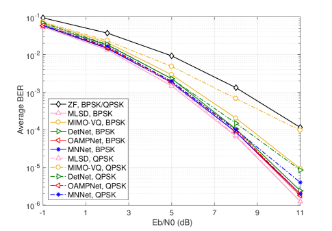
Figure 9: BER as a function of $E_{b}/N_{0}$ for different detection algorithms in uncoded 4-by-8 MIMO system with BPSK/QPSK modulation.

Fig. 9 illustrates the average BER performance of different detection algorithms in uncoded 4-by-8 MIMO system with BPSK/QPSK modulation. It is observed that all of the deep learning algorithms outperform the conventional ZF algorithm throughout the whole SNR range. Specifically, the MIMO-VQ model has its performance quickly moved away from the optimum due to the increasing number of transmit antennas. The performance degraded around 1 dB for BPSK and 3.2 dB for QPSK. DetNet achieves a good performance on BPSK, but its performance gap with MLSD increases to 1.7 dB when we move to QPSK. Meanwhile, OAMPNet and MNNet approaches are both very close to optimum for BPSK modulation over the whole SNR range. The performance of MNNet slightly decreased as we move to QPSK; the performance gap to MLSD is around 0.4 dB at BER of $10^{-5}$. Despite, the proposed MNNet does not require matrix inversion which makes it more advantage in terms of computational complexity.

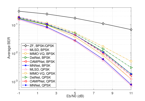
Figure 10: BER as a function of $E_{b}/N_{0}$ for different detection algorithms in uncoded 4-by-4 MIMO system with BPSK/QPSK modulation.

Fig. 10 illustrates the average BER performance of different detection algorithms in uncoded 4-by-4 MIMO system with BPSK/QPSK modulation. Similar results have been observed since all of the deep learning based algorithms largely outperform ZF receiver across different modulation schemes over a wide range of SNR s. For BPSK modulation, DetNet with its performance gap between MLSD around 1 dB at BER of $10^{-2}$; simple MIMO-VQ achieves a slightly better performance with a gap around 0.8 dB. OAMPNet and MNNet are both very close to optimum performance at whole SNR range. For QPSK modulation, DetNet outperforms MIMO-VQ with a performance improvement approximately 0.5 dB at BER of $10^{-2}$. Meanwhile, OMAPNet and MNNet both achieve near-optimum performance and OMAPNet slightly outperforms MNNet at high SNR range with a performance gap less than 0.2 dB.

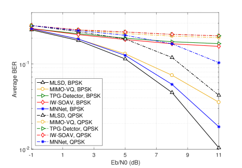
Figure 11: BER as a function of $E_{b}/N_{0}$ for different detection algorithms in uncoded 8-by-4 MIMO system with BPSK/QPSK modulation.

Fig. 11 illustrates the average BER performance of different detection algorithms in uncoded 8-by-4 MIMO system with BPSK/QPSK modulation. The baselines for performance comparison including MLSD, IW-SOAV and TPG-Detector. Here we do not employ any channel-inversion based algorithms (e.g. ZF and OAMPNet) due to matrix singularity. For BPSK, it is observed that simple MIMO-VQ is able to outperform both IW-SOAV and TPG-Detector; and the proposed MNNet algorithm further improves the performance of MIMO-VQ model for approximately 1.7 dB at high SNR range. Beside, the gap between MNNet and MLSD is around 1 dB. However, its performance gap with MLSD increases as we move to QPSK (e.g. around 2.3 dB at BER of $10^{-1}$). Meanwhile, the other three approaches almost fail to detect with an error floor at high SNR range due to system outage.

VI Conclusion

In this paper, we have intensively studied fundamental behaviors of the ANN-assisted MIMO detection. It has been revealed that the ANN-assisted MIMO detection is naturally a MIMO-VQ procedure, which includes joint statistical channel quantization and message quantization. Our mathematical work has shown that the quantization loss of MIMO-VQ grows linearly with the number of transmit antennas; and due to this reason, the ANN-assisted MIMO detection scales poorly with the size of MIMO. To tackle the scalability problem, we investigated a MNN based MIMO-VQ approach, named MNNet, which can take the advantage of PIC to scale up the MIMO-VQ on each super layer, and consequently the whole network. Computer simulations have demonstrated that the MNNet is able to achieve near-optimum performances in a wide range of communication tasks. In addition, it is shown that a well-modularized network architecture can ensure better computation efficiency in both the ANN training and evaluating procedures.

References

- [1] A. J. Paulraj, D. A. Gore, R. U. Nabar, and H. Bolcskei, “An overview of MIMO communications - a key to gigabit wireless,” Proceedings of the IEEE, vol. 92, no. 2, pp. 198–218, Feb. 2004.
- [2] T. J. O’Shea, T. Erpek, and T. C. Clancy, “Deep learning based MIMO communications,” CoRR, vol. abs/1707.07980, 2017.
- [3] Q. Mao, F. Hu, and Q. Hao, “Deep learning for intelligent wireless networks: A comprehensive survey,” IEEE Communications Surveys Tutorials, vol. 20, no. 4, pp. 2595–2621, Fourthquarter 2018.
- [4] M. Chen, U. Challita, W. Saad, C. Yin, and M. Debbah, “Artificial neural networks-based machine learning for wireless networks: A tutorial,” IEEE Communications Surveys Tutorials, vol. 21, no. 4, pp. 3039–3071, Fourthquarter 2019.
- [5] N. Samuel, T. Diskin, and A. Wiesel, “Learning to detect,” IEEE Transactions on Signal Processing, vol. 67, no. 10, pp. 2554–2564, May 2019.
- [6] S. Takabe, M. Imanishi, T. Wadayama, and K. Hayashi, “Trainable projected gradient detector for massive overloaded MIMO channels: Data-driven tuning approach,” CoRR, vol. abs/1812.10044, 2018.
- [7] H. He, C. Wen, S. Jin, and G. Y. Li, “A model-driven deep learning network for MIMO detection,” in 2018 IEEE GlobalSIP, Nov. 2018, pp. 584–588.
- [8] Y. Liu, S. Bi, Z. Shi, and L. Hanzo, “When machine learning meets big data: A wireless communication perspective,” CoRR, vol. abs/1901.08329, 2019.
- [9] Y. Takefuji, Neural Network Parallel Computing. Norwell, MA, USA: Kluwer Academic Publishers, 1992.
- [10] J. Park, S. Samarakoon, M. Bennis, and M. Debbah, “Wireless network intelligence at the edge,” CoRR, vol. abs/1812.02858, 2018.
- [11] A. Yazar and H. Arslan, “Reliability enhancement in multi-numerology-based 5G new radio using INI-aware scheduling,” EURASIP Journal on Wireless Communications and Networking, vol. 2019, no. 1, p. 110, May 2019.
- [12] N. Kim, Y. Lee, and H. Park, “Performance analysis of MIMO system with linear MMSE receiver,” IEEE Trans. Wireless Commun., vol. 7, no. 11, pp. 4474–4478, Nov. 2008.
- [13] P. Li, R. C. de Lamare, and R. Fa, “Multiple feedback successive interference cancellation detection for multiuser MIMO systems,” IEEE Trans. Wireless Commun., vol. 10, no. 8, pp. 2434–2439, Aug. 2011.
- [14] S. M. Razavizadeh, V. T. Vakili, and P. Azmi, “A new faster sphere decoder for MIMO systems,” in Proceedings of the 3rd IEEE ISSPIT, Dec. 2003, pp. 86–89.
- [15] F. Rusek, D. Persson, B. K. Lau, E. G. Larsson, T. L. Marzetta, O. Edfors, and F. Tufvesson, “Scaling up MIMO: Opportunities and challenges with very large arrays,” IEEE Signal Process. Mag., vol. 30, no. 1, pp. 40–60, Jan. 2013.
- [16] L. Van der Perre, L. Liu, and E. G. Larsson, “Efficient DSP and circuit architectures for massive MIMO: State of the art and future directions,” IEEE Trans. Signal Process., vol. 66, no. 18, pp. 4717–4736, Sep. 2018.
- [17] T. O’Shea and J. Hoydis, “An introduction to deep learning for the physical layer,” IEEE Trans. Cogn. Commun. Netw., vol. 3, no. 4, pp. 563–575, Dec. 2017.
- [18] S. Xue, Y. Ma, A. Li, N. Yi, and R. Tafazolli, “On unsupervised deep learning solutions for coherent MU-SIMO detection in fading channels,” in 2019 IEEE Int. Conf. Commun., May 2019, pp. 1–6.
- [19] S. Yang and L. Hanzo, “Fifty years of MIMO detection: The road to large-scale MIMOs,” IEEE Commun. Surveys Tuts., vol. 17, no. 4, pp. 1941–1988, Fourthquarter 2015.
- [20] D. S. Poznanovic, “The emergence of non-von neumann processors,” in Reconfigurable Computing: Architectures and Applications. Berlin, Heidelberg: Springer Berlin Heidelberg, 2006, pp. 243–254.
- [21] D. M. Hawkins, “The problem of overfitting,” Journal of Chemical Information and Computer Sciences, vol. 44, no. 1, pp. 1–12, 2004, pMID: 14741005.
- [22] Y. C. Youngseok Lee, Kyoungae Kim, “Optimization of AP placement and channel assignment in wireless LANs,” in 27th Annual IEEE Conf. on LCN, Nov. 2002, pp. 831–836.
- [23] C. Rudin, “Stop explaining black box machine learning models for high stakes decisions and use interpretable models instead,” Nat. Mach. Intell., vol. 1, pp. 206–215, May 2019.
- [24] D. Castelvecchi, “Can we open the black box of AI?” Nature, vol. 538, pp. 20–23, Oct. 2016.
- [25] A. Adadi and M. Berrada, “Peeking inside the black-box: A survey on explainable artificial intelligence,” IEEE Access, vol. 6, pp. 52 138–52 160, 2018.
- [26] S. C. Ahalt and J. E. Fowler, “Vector quantization using artificial neural network models,” in Int. Workshop Adaptive Methods and Emergent Tech. for Signal Process. and Commun., Jun. 1993, pp. 42–61.
- [27] A. Gersho and R. M. Gray, Vector Quantization and Signal Compression. Kluwer international series in engineering and computer science, Norwell, MA, 1992.
- [28] D. O. Hebb, The organization of behavior: A neuropsychological theory. New York: Wiley, Jun. 1949.
- [29] N. M. Nasrabadi and Y. Feng, “Vector quantization of images based on the Kohonen self-organizing feature maps,” in IEEE Int. Conf. Neural Netw., Jul. 1988, pp. 101–108.
- [30] T. Kohonen, “The self-organizing map,” Proc. of the IEEE, vol. 78, pp. 1464–1480, Sep. 1990.
- [31] S. Grossberg, “Adaptive pattern classification and universal recoding: Part I. parallel development and coding of neural feature detectors,” Biological Cybernetics, vol. 23, pp. 121–134, 1976.
- [32] J. C. De Luna Ducoing, Y. Ma, N. Yi, and R. Tafazolli, “A real complex hybrid modulation approach for scaling up multiuser MIMO detection,” IEEE Trans. Commun., vol. 56, pp. 3916–3929, Sep. 2018.
- [33] J. M. Keller, M. R. Gray, and J. A. Givens, “A fuzzy k-nearest neighbor algorithm,” IEEE Trans. Syst., Man, Cybern., vol. SMC-15, no. 4, pp. 580–585, Jul. 1985.
- [34] J. P. Theiler and G. Gisler, “Contiguity-enhanced k-means clustering algorithm for unsupervised multispectral image segmentation,” in Algorithms, Devices, and Systems for Optical Information Processing, vol. 3159, International Society for Optics and Photonics. SPIE, 1997, pp. 108 – 118.
- [35] N. M. Nasrabadi and R. A. King, “Image coding using vector quantization: a review,” IEEE Trans. Commun., vol. 36, no. 8, pp. 957–971, Aug. 1988.
- [36] A. C. Bovik, Handbook of Image and Video Processing. Orlando, FL, USA: Academic Press, Inc., 2005.
- [37] I. Goodfellow, Y. Bengio, and A. Courville, Deep Learning. MIT Press, 2016.
- [38] B. L. Happel and J. M. J. Murre, “The design and evolution of modular neural network architectures,” Neural Networks, vol. 7, pp. 985–1004, 1994.
- [39] M. Latva-aho and J. Lilleberg, “Parallel interference cancellation in multiuser detection,” in Proceedings of International Symposium on Spread Spectrum Techniques and Applications, vol. 3, Sep. 1996, pp. 1151–1155.
- [40] J. Schmidhuber, “Deep learning in neural networks: An overview,” Neural Networks, vol. 61, pp. 85–117, 2015.
- [41] D. E. Rumelhart, R. Durbin, R. Golden, and Y. Chauvin, “Backpropagation.” Hillsdale, NJ, USA: L. Erlbaum Associates Inc., 1995, ch. Backpropagation: The Basic Theory, pp. 1–34.
- [42] M. A. Riedmiller, “Advanced supervised learning in multi-layer perceptrons - from backpropagation to adaptive learning algorithms,” Computer Standards and Interfaces, vol. 16, pp. 265–278, 1994.
- [43] L. Luo, Y. Xiong, and Y. Liu, “Adaptive gradient methods with dynamic bound of learning rate,” in International Conference on Learning Representations, 2019.
- [44] S. G. Kim, D. Yoon, S. K. Park, and Z. Xu, “Performance analysis of the MIMO zero-forcing receiver over continuous flat fading channels,” in The 3rd International Conference on Information Sciences and Interaction Sciences, June 2010, pp. 324–327.
- [45] A. H. Mehana and A. Nosratinia, “Diversity of MMSE MIMO receivers,” CoRR, vol. abs/1102.1462, 2011.
- [46] Y. Hama and H. Ochiai, “Performance analysis of matched filter detector for MIMO systems in rayleigh fading channels,” in GLOBECOM 2017 - 2017 IEEE Global Communications Conference, Dec 2017, pp. 1–6.
- [47] R. Hayakawa, K. Hayashi, H. Sasahara, and M. Nagahara, “Massive overloaded MIMO signal detection via convex optimization with proximal splitting,” in 2016 24th European Signal Processing Conference (EUSIPCO), Aug 2016, pp. 1383–1387.