Multi-Photon Synthetic Lattices in Multi-Port Waveguide Arrays: Synthetic Atoms and Fock Graphs
Abstract
Activating transitions between internal states of physical systems has emerged as an appealing approach to create lattices and complex networks. In such a scheme, the internal states or modes of a physical system are regarded as lattice sites or network nodes in an abstract space whose dimensionality may exceed the systems’ apparent (geometric) dimensionality. This introduces the notion of synthetic dimensions, thus providing entirely novel pathways for fundamental research and applications. Here, we analytically show that the propagation of multi-photon states through multi-port waveguide arrays gives rise to synthetic dimensions where a single waveguide system generates a multitude of synthetic lattices. Since these synthetic lattices exist in photon-number space, we introduce the concept of pseudo-energy and demonstrate its utility for studying multi-photon interference processes. Specifically, the spectrum of the associated pseudo-energy operator generates a unique ordering of the relevant states. Together with generalized pseudo-energy ladder operators, this allows for representing the dynamics of multi-photon states by way of pseudo-energy term diagrams that are associated with a synthetic atom. As a result, the pseudo-energy representation leads to concise analytical expressions for the eigensystem of photons propagating through nearest-neighbor coupled waveguides. In the regime where and , non-local coupling in Fock space gives rise to hitherto unknown all-optical dark states which display intriguing non-trivial dynamics.
I Introduction
The concept of synthetic dimensions has recently opened the door to novel perspectives for
expanding the dimensionality of well-understood physical systems
Juki2013 ; Yuan2016 ; Bilitewski2016 ; Ozawa2016 ; Fan2017 .
One strategy to explore synthetic dimensions consists in driving the associated dynamical
systems in order to activate the coupling between different internal modes which under normal
conditions remain uncoupled
Yuan2018 .
By doing so, the resulting coupled modes exhibit lattice-like structures that exist in an
abstract space which is nonetheless physical.
The importance of synthetic lattices lies on the fact that they allow us to explore a variety
of effects that are not available in spatial or temporal domains.
To illustrate the basic idea of activating synthetic dimensions, and to set the stage for
the present work, we begin by elucidating how a one-dimensional quantum harmonic oscillator
generates a lattice in Fock space.
The oscillator’s Hamiltonian is given as ,
and its dynamics is governed by the Schrödinger equation .
Here, is the angular frequency of the oscillator, and and
denote, respectively, the annihilation and creation operators
Louisell .
Notice, we have set the reduced Planck constant and the oscillator mass to unity,
i.e., and . When the oscillator is initially prepared in the eigenstate
, then it will remain in this state, only acquiring a time-dependent
phase factor during evolution, i.e., .
No transitions to other eigenstates occur.
However, by subjecting the oscillator to a time-dependent displacement,
, the Hamiltonian acquires
the form .
Substituting the general state vector -
where are the transition amplitudes from the initial
state to the final state and is the time evolution operator - into the Schrödinger equation, we find
that the amplitudes obey the semi-infinite set of coupled differential equations
| (1) | ||||
| (2) |
These equations clearly illustrate that the time dependent displacement
activates transitions between the amplitudes , , and .
This implies that in Fock space the oscillator generates a lattice, where it can
”hop” from eigenstate to the adjacent eigenstates and
with hopping rates and , respectively
PhysRevA.95.023607 ; Apleija2010 ; Keil2011 ; Apleija2012 ; Keil2012 ; Nezhad2013 ; Wang2016 .
In general, applying dynamic modulations to the potentials associated with physical
systems induces coupling among the supported eigenstates. Using this technique, a
photonic topological insulator in synthetic dimensions has been recently implemented
via modulated waveguide lattices Eran ; Ozawa2019 .
Synthetic dimensions have also been explored in harmonic traps Price2017 ,
optical lattices Wang2015 , cavities Wang2016 and even in room-temperature Rydberg atoms Cai2019 .
Within the realm of optics and photonics, synthetic dimensions can be created by
exploiting the spatial, temporal, polarization, and frequency degrees of freedom
of light Yuan2018 .
For instance, large-scale parity-time symmetric lattices have been implemented in
the temporal domain using optical fiber loops endowed with gain and loss Regensburger2 ; Regensburger1
and a driven-dissipative analogon of the four-dimensional quantum Hall effect has
been observed in a spatially 3D resonator lattice Ozawa2016 .
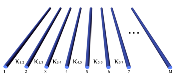
In this work, we show that high-dimensional lattices emerge in photon-number space
when a photonic lattice of ports Longhi2009 ; Szameit2010
is excited by indistinguishable photons, see Fig. (1).
More precisely, the Fock-representation of -photon states in systems composed
of evanescently coupled single-mode waveguides yields to a new layer of
abstraction where the associated states can be visualized as the energy levels
of a synthetic atom that features a number of allowed and disallowed
transitions between its energy levels.
In photonic waveguide lattices, where all the waveguides are coupled to each other, the quantum optical Hamiltonian in paraxial approximation is given as
Chak2007 ,
where and , respectively, are bosonic creation
and annihilation operators for photons in the -th waveguide. Further,
denotes the propagation constant of the -th waveguide and
is the coupling coefficient between the -th and -th
waveguide.
For simplicity we restrict our subsequent analysis to the simplest scenario of
(in real space) essentially one-dimensional waveguide arrays with nearest-neighbor
couplings
| (3) |
Under these premises, the propagation of a single-photon along the waveguide can be described using the Heisenberg equations of motion for the bosonic creation operators Lai1991 ; Bromberg2009
| (4) |
where . Accordingly, the single-photon response is computed through the input-output transformation , where denotes the matrix element of the evolution operator Markus2016 . Using this formalism, it is straightforward to show that an initial -photon state , with , will transform into the output state
| (5) | |||
In the context of waveguide lattices, the input-output formalism is by far the most common approach used to compute the output states MarkusReview .
Nonetheless, as we will demonstrate in the remainder of the manuscript, the input-output scheme fails to expose the intrinsic coupling interactions between
the emerging states.
In what follows, we use the equivalent Schrödinger-picture formalism to unveil
the high-dimensional lattice structures arising from the propagation of multiple
photons through multi-port waveguide systems. To do so, we first notice that
indistinguishable photons exciting coupled waveguides, give rise to a total
of states which are given by all permutations of the
integer partitions of among the sites.
For the trivial case of photon, we simply obtain a set of states
| (6) |
with . By computing the matrix elements of the Hamiltonian given in (3) for , , one can readily see that the single-photon states are coupled to each other as displayed by the equations
| (7) |
in agreement with (4).
We now consider the more interesting scenario of photons propagating through a
waveguide beam splitter, , with propagation constants and
and symmetric coupling, i.e., .
In this case, there exists a total of states, namely ,
and the Hamiltonian given in (3) acquires the form
| (8) |
Computing the matrix elements reveals that the states obey the equations of motion
| (9) | ||||
with and Tschernig:18 . This indicates that
inside a waveguide beam splitter the amplitudes of two-mode -photon states evolve
coupled to each other with hopping rates , and the corresponding phases depend
on both propagation constants.
For the case of two identical waveguides we have so
that the first term on the r.h.s. of (9) becomes
which indicates that all the states will exhibit the same effective propagation
constant.
Interestingly, it has been recently shown that waveguide beam splitters produce the
Discrete Fractional Fourier Transform (DFrFT) of -photon states
Tschernig:18 , as well as exceptional points of arbitrary order, provided that losses are introduced
in one of the waveguides Quiroz-Juarez:19 .
On the other hand, when considering two non-identical waveguides, , the first term on the r.h.s. of (9) acquires the form
.
Remarkably, the term indicates that the state evolution will be influenced by an effective ramping potential in the same
fashion as in the case of classical waves in Bloch oscillator systems Silberberg1999 ; Keil2012 ; Lebugle2015 .
Consequently, we can tailor the dynamics of -photon states by simply adjusting
the Bloch slope in order to suppress and/or create
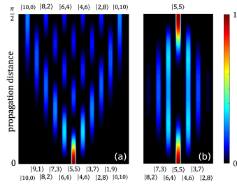
certain output states. As an illustration, we depict in Figure 2 the
probability evolution for the initial state in a waveguide beam splitter
with coupling coefficient (a) for and (b) for
. While case (a) corresponds to discrete ”diffraction”
of the initial state in state space, case (b) corresponds to ”Bloch oscillations”
in state space.
Note, that throughout this work we present all simulations using the normalized
propagation coordinate , where is the actual propagation distance
and stands for the nearest-neighbor coupling coefficient.
After the above introductory examples, we now proceed to consider the most interesting
case where multiple photons excite more than two waveguides . In order to
motivate the concept of pseudo-energy we first examine the simplest case of a waveguide
trimer, , that is excited by photons and then move on to the general case.
For a waveguide trimer and two identical photons, the Hamiltonian takes the form
| (10) |
In this scenario, we have a total of 6 photon-number states obeying the following coupled set of equations of motion
| (11) | ||||
| (12) | ||||
| (13) | ||||
| (14) | ||||
| (15) | ||||
| (16) | ||||
| (17) | ||||
| (18) |
As in the earlier examples, here we also have the possibility of molding the state dynamics via tuning the propagation constants and coupling coefficients.
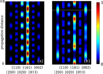
For instance, for equal coupling coefficients and identical
waveguides , we observe a periodic spreading and contraction
of the two-photon wave function, as illustrated in Figure 3 (a).
In contrast, choosing a different propagation constant for the central waveguide,
, leads to a quasi-periodic evolution, Figure 3 (b).
Indeed, this quasi-periodic evolution occurs because the ratios between the
eigenvalues of the coupling matrix are irrational numbers. We would like to
emphasize that at the propagation distance indicated by the dashed line in
Figure 3 (b), the input state evolves into a quasi
two-photon N00N state in state space, which is reminiscent of the Hong-Ou-Mandel
effect
Hong1987 .
To describe the photon dynamics in the waveguide trimer, we have obtained an
even number of equations. At this point, the way in which the states should
be arranged into a synthetic lattice is not at all clear.
To be precise, the six states representing the sites of the synthetic lattice
can be sorted into at least two distinct natural sequences as shown in
Table 1.
Clearly, arranging the states into a lattice (i.e., sorting) and analyzing the corresponding equations of motion becomes rather cumbersome when considering higher photon numbers in multiple coupled waveguides. In the following section, we, therefore, introduce a concise and universal method that facilitates studying the general case of photons propagating in arrays formed by waveguides. The resulting structures follow from physical and mathematical considerations that eventually allow us to describe multi-photon processes in waveguide arrays in a surprising and remarkable way that resembles the quantum-mechanical description of multi-level atoms.
II Pseudo energy representation
We now introduce a concept analogous to the concept of energy and we, therefore,
refer to it as the pseudo-energy. As we show below, the concept of
pseudo-energy is rather useful since it facilitates a unique sorting
of multi-photon Fock states in a physically meaningful way and allows for
establishing a correspondence between Fock states and the energy levels of a
synthetic atom.
Concurrently, we identify pseudo-energy ladder operators along with
pseudo-exchange-energies in order to define the corresponding selection
rules in Fock space for transitions between the pseudo-energy levels
of the synthetic atom.
We consider indistinguishable photons propagating in an array of
lossless evanescently coupled waveguides that give rise to
Fock states , fulfilling the condition .
The first issue to be addressed is to determine a way of sorting the multi-photon
states in Fock space in a meaningful way. To do so, we associate a unique
numerical value to every state as follows
| (19) |
Here, the subscript indicates that the numbers in the square brackets have to be expressed in base , and the least significant digit is the left-most number . Observing that allows us to define the pseudo-energy operator
| (20) |
such that its action on the -photon--mode Fock states yields
| (21) |
with eigenspectrum .
From (21), we readily infer the smallest and largest eigenvalues
and
,
respectively.
Accordingly, the eigenvalues are bounded by .
As a result, in order to sort the associated Fock states, we have to compute
the corresponding ’s and arrange them in ascending order. The resulting
ladder of ’s then defines the synthetic lattices formed by the states.
We refer to this ordering as the pseudo-energy representation of the
-photon--mode Fock states.
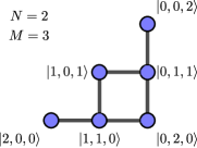
For illustration, we revisit the above case of photons propagating in an
array of waveguides. Accordingly, there are states and the
spectrum of the pseudo-energy operator comprises integers
| (22) |
Using these numbers we readily obtain the pseudo-energy representation of the 2-photon-3-mode Fock space
| (23) | ||||
Consequently, we designate as the pseudo-energy of the -th Fock state in the -photon--mode Fock space
| (24) |
with . In general, for any given and pseudo-energy , the inverse mapping onto the mode-occupation numbers is
| (25) |
where the symbol corresponds to integer division and is
the modulo operator.
We now proceed to show how the pseudo energy representation of Fock states
allows us to express the equations of motion of photons in waveguides
in a concise way. To do so, we take a closer look at the action of the
operator on a Fock state
| (26) |
If the state corresponds to the pseudo-energy , then the resulting state on the r.h.s. of (26) must have the pseudo-energy
| (27) | ||||
Therefore, the action of changes the pseudo-energy of Fock states by the amount
| (28) |
which we denote as the pseudo-exchange energy associated with the tunneling process taking place between waveguides and . In this sense the operators can be thought of as pseudo-energy ladder operators, which raise or lower the pseudo-energy of Fock states. Consequently, we can write
| (29) |
The physical significance of (29) is that a direct transition between the states and is only possible if there exists a pseudo-exchange energy such that
| (30) |
Obviously, (30) defines the selection rules in Fock space. Together with the action of the photon number operators , the full system of coupled equations governing the propagation of photons through coupled waveguides in the pseudo-energy representation is given by
| (31) |
For the case of nearest-neighbour coupled, identical waveguides, where all the propagation constants are the same, the relevant pseudo-exchange energies are and the set of coupled equations reduces to
| (32) | ||||
To further illustrate the resulting coupling system in Fock space, we revisit the
case of a single photon propagating in waveguides. The effective coupling
behavior - of allowed and forbidden transitions in Fock space - can now be visualized
within a pseudo-energy term diagram, as illustrated in Figure 4 (a).
In this particular case the nearest-neighbour coupling of the waveguides is retained
in Fock space and any given Fock state only couples to its nearest
neighbours .
A similar picture arises in the case of two waveguides and photons, as
depicted in Figure 4 (b). Here, we obtain a term-diagram that is
essentially isomorphic to Figure 4 (a), where – again – only
nearest-neighbour Fock states are coupled to each other.
The nearest neighbour picture radically changes when applying the pseudo-energy
approach to the case of photons and waveguides as displayed in the
corresponding term-diagram in Figure 4 (c). Importantly, even
when the waveguides are – in real space – only coupled to their nearest
neighbors, in photon number space certain states become coupled to next-nearest
neighbor states.
For instance, in Figure 4 (c) we observe that the state
not only couples to its neighbors
and , but
also to the next-nearest neighbour state .
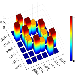
For illustrative purposes, we present in Figure 5 the coupling
matrix for this particular set of states when the three-waveguide system is
formed by identical waveguides, , and balanced coupling
coefficients .
At this point is rather evident that the richness and complexity of the emerging
synthetic configurations will become more prominent when higher number of photons
and waveguides are considered. Moreover, it is worth stressing that in order to
generate the present synthetic structures we did not require any modulation of
the system parameters as the states naturally couple due to the system’s internal
dynamics.

III Non-planar synthetic lattices: Fock graphs
In this section we introduce a more convenient way of representing the hamiltonian matrix of -photons exciting -waveguides. To do so, we interpret the states as vertices of a graph (Fock graph) where the allowed inter-state transitions represent the edges. A practical representation of finite graphs is the so-called adjacency matrix whose entries indicate whether pairs of vertices are adjacent or not. In the present context, the effective Hamiltonian in the -photon--mode pseudo-energy representation determines such an adjacency matrix
| (33) |
where is the step-function and indicates
a connection (or no connection) between the vertices and . In what follows,
we assume identical waveguides with in order to omit self-loops
in the graph representation. As an example, in Figure 6 we depict the Fock
graph arising from the effective Hamiltonian of Figure 5, which we have
already discussed in the previous section.
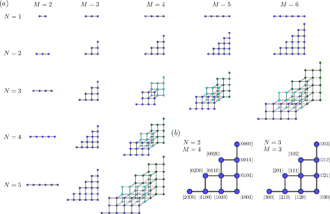
In Figure 7 (a), we depict further examples for photon numbers up to
and up to waveguides. The first row, which corresponds to single photon graphs,
simply reflects the one-dimensional spatial configuration of the waveguides. By introducing
a second photon, we observe that the Fock graphs become two-dimensional, Figure 7 (b),
except for the case . The inclusion of more photons leads to non-planar graphs, i.e. graphs that cannot be drawn in 2D without intersecting edges, which
exhibit a layered structure in three dimensions as indicated by the different coloring
of the nodes in different layers.
A prominent feature to highlight is the symmetry observed among graphs emerging for
the combinations and and for and , where
is an integer.
In other words, every Fock graph has an isomorphic partner graph
| (34) |
with an identical adjacency matrix, up to a trivial permutation of the node labels.
In Figure 7 (b), we depict the smallest non-trivial pair of Fock
graphs and the corresponding adjacency matrices that are induced by the pseudo-energy
representation. If we were to start from and permute its rows
and columns according to
we will exactly obtain .
Indeed, this underlying symmetry in the space of possible Fock graphs has very
interesting implications. For instance, in
Ref. Tschernig:18
we have shown that it is possible to implement the number-resolved -dimensional
Discrete Fractional Fourier Transform (DFrFT) with a single waveguide beam splitter by
launching indistinguishable photons. Furthermore, using the same photon-number-resolved
mapping in Ref. Quiroz-Juarez:19
we have shown how to attain so-called exceptional points of order, by way
of exciting a semi-lossy waveguide beam splitter with high photon number states.
In fact, it is now clear that these results emerge as special cases of
(34), which pertains to the identity of the first row and
column in Figure 7 (a). Thus, by following similar ideas it is
possible, in principle, to find the corresponding effects for waveguide systems
with excited by photons.
Additionally, by exploiting the graph symmetry it becomes apparent that a specific
transformation which requires photons and waveguides could likewise be
implemented with photons and waveguides. Of course, such alternative
pathways of implementing a transformation are not always guaranteed because of
the different dimensions of the experimentally accessible parameter spaces.
Nonetheless, this may serve as a useful Ansatz to overcome concrete experimental
difficulties.
Quite interestingly, synthetic Fock lattices have been
explored previously in the context of QED circuits by Wang et al. Wang2016 .
In such a study, the joint excitation states of an atom coupled to the -photon -cavity
Fock space form a two-dimensional, hexagonal Haldane-like synthetic lattice, which facilitates
the generation of high photon-number NOON states. Crucially, the realization of this scheme demands the judicious implementation of the coupling between atom and cavity, as well as the precise modulation of the cavity resonance frequencies.
In contrast, the multi-photon synthetic dimensions explored in the present work are intrinsically active by virtue of the indistinguishability of the photons,
and as such they do not require any external driving of the system’s parameters.
The Fock graphs offer a rich variety of synthetic coupled structures. This variety
can be further enhanced by considering different spatial arrangements of the
waveguides, for instance, ring- or star-shaped structures instead of the simple
planar configuration studied here.
Importantly, the evolution of multi-photon states in synthetic lattices and graphs can be dynamically reconfigured by using programmable photonic chips Shadbolt2012 . That is, integrated optical devices where the waveguides’ refractive index and coupling coefficients can be modified externally.
Nevertheless, even with this simple one-dimensional arrangement comprising a few waveguides, small photon numbers, and a time-independent Hamiltonian,
one encounters interesting effects that are only possible due to the multi-dimensionality of the corresponding Fock graphs.
IV All-optical dark states and parallel quantum random walks
To show possible applications of the pseudo-energy synthetic lattices we discuss the generation of all-optical dark states Lambropoulos2007 and multi-photon quantum. The simplest dark states are encountered in 3-level atomic- or molecular systems, where radiative transitions between, e.g.,
are allowed but the transition
is forbidden. In this simple scenario, a dark state is
a superposition of the uncoupled states ,
where is given in terms of the Rabi frequencies of the allowed transitions Lambropoulos2007 .
Once the system is in such a state, adiabatic changes in the Rabi frequencies allow for the tuning of
the populations of the states and , while the probability of remains 0.
This ineresting behavior, which seemingly evades the radiative selection rules, can be mimicked in the pseudo-energy representation of Fock states using our all-optical setup.
To do so, we revisit one more time the case of waveguides, with equal propagation constants and balanced coupling coefficients , excited by photons. The pseudo-energy representation of the effective Hamiltonian takes the form
| (35) |
With this choice of parameters the spectrum of is integer-valued
| (36) |
which indicates that the third and fourth eigenstates are degenerate with eigenvalues . We now consider the evolution of a coherent superposition of the eigenstates
| (37) |
with corresponding eigenvalues and , specifically
| (38) |
In the standard Fock representation reads as
| (39) |
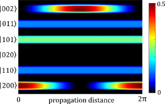
The probability evolution for this state is shown in Figure 8.
As one can see, this state displays the characteristic behavior of a dark state. That is, the initial state evolves exhibiting oscillating transitions between the states and with period . These transitions occur in spite of the fact that direct transition is forbidden , and those states have the maximum
possible distance within the graph, that is, at least 4 single-photon tunneling processes are required to transform one state into the other. All probabilities of the intermediate states remain constant and, in a way, assist the simultaneous tunneling of two photons between the outermost waveguides. We stress that this 6-level dark-state state is induced by a time-independent hamiltonian and it occurs naturally without the need of adiabatic fine-tuning of the parameters. We would further like to note, that the
state exhibits zero probability for all , further attesting a
multi-photon tunneling (in this case co-tunneling) effect taking place between
the two waveguides.
Geometrically speaking, this effect arises due to destructive interference taking
place in the two-way branching of the Fock graph shown in Figure 6.
This branching effectively allows for the flow of the amplitudes to take a
‘detour’ around the node.
As an alternative, one may attempt to implement a real space structure in one
or two dimensions consisting of six coupled waveguides in order to emulate an
equivalent Hamiltonian for just a single photon. However, this would be topologically
impossible, since there always exist additional cross-talk between the waveguides
representing the nodes at the center of the graph. In other words, our Fock-graph
based analysis of multi-photon propagation in waveguide arrays allows the realization
of functionalities beyond what can be realized with linear (single-photon) based
networks.
Quite interestingly, by exciting waveguide lattices with multi-photon states
comprising infinite coherent superpositions, e. g. coherent states
or two-mode squeezed vacuum states ,
opens a route to generating, in principle, an infinite number of lattices or
graphs with different numbers of lattice sites and many dimensions simultaneously.
This possibility is very appealing for realizing parallel quantum random walks
where the corresponding walkers can perform different numbers of steps that
depend on the number of photons involved in each process. We stress that the
observation of these quantum walks is nowadays possible utilizing bright
parametric down-conversion sources in combination with photon-number-resolving
detectors Magana2019 .
V Eigendecomposition in the pseudo-energy representation
In this final section, we obtain an analytical expression for the eigensystem of an waveguide system (or tight-binding network) with arbitrary coupling coefficients excited by indistinguishable photons. With the help of the pseudo-energy representation we will be able to find a concise expression, which also introduces a natural ordering of the -photon--waveguide eigenstates. As we have seen, in the case of a single photon , the Hamiltonian takes on a bi-diagonal form in the pseudo-energy representation. In some cases it is possible to find an analytical closed form expression for the eigensystem, as for example in the case of the DFrFT Weimann2016 . Even if no analytical solution is available, numerical algorithms are known Gill1990 , that deal with bi-diagonal matrices efficiently. Therefore, without loss of generality we assume that we know the complete eigensystem of the single-photon--waveguide Hamiltonian, which we denote as
| (40) | ||||
| (41) |
where . In the above equation, is the -th component of the -th eigenvector of the matrix and it defines the single-particle eigenstates
| (42) |
When the same waveguide system is excited by photons, it is clear that the many-particle eigenstates arise from the tensor-products of the single-particle eigenstates. Formally, we may write the resulting states as
| (43) |
but now the occupation numbers pertain to the number of photons occupying the -th single-particle eigenmode. Consequently, we can apply the pseudo-energy ordering to the -particle eigenstates by defining . The -th eigenstate of the -photon system is then given by
| (44) |
Note, that in most cases it is necessary to normalize the resulting expression on the r.h.s. of (44). By requiring , where denotes -photon--waveguide Fock states, we find for the components
| (45) |
It is now rather straightforward to show, that the -particle eigenvalues are given as the sum of the eigenvalues of the involved single-particle eigenstates
| (46) |
Using (44) and (6) it is straightforward to find the -photon--waveguide time-evolution operator . We would like emphasize that the numerical evaluation of (44) is far more efficient than the direct diagonalization of the full matrix representation of in -photon--waveguide Fock space. Due to the size and highly non-trivial structure of the resulting matrices, general eigensystem-solvers produce a significant amount of overhead, which we avoid in our approach. Essentially, we do not even require a calculation of the full matrix representation . Instead, knowledge of the single-particle eigensystem and the bosonic nature of photons suffices.
VI Conclusion
In summary, we have shown that the propagation of multi-photon states through multi-port waveguide systems (tight-binding networks) gives rise to multiple synthetic lattices and multi-dimensional Fock graphs that allow for transparent analyses of the relevant physical processes and the design of novel functionalities beyond the linear (single-photon) realm. Since such synthetic structures emerge in the photon-number space we have been able to associate coherent multi-photon processes to parallelized multi-dimensional quantum random walks. This parallelization brings about novel opportunities for the implementation of random walks where the randomness is not only present in the dynamics of the walkers but also in the simultaneous occurrence of different walks.
Acknowledgments
We acknowledge support by the Deutsche Forschungsgemeinschaft (DFG) within the framework of the DFG priority program 1839 Tailored Disorder.
References
- [1] D. Jukić and H. Buljan. Four-dimensional photonic lattices and discrete tesseract solitons. Phys. Rev. A, 87:013814, Jan 2013.
- [2] Luqi Yuan, Yu Shi, and Shanhui Fan. Photonic gauge potential in a system with a synthetic frequency dimension. Opt. Lett., 41(4):741–744, Feb 2016.
- [3] Thomas Bilitewski and Nigel R. Cooper. Synthetic dimensions in the strong-coupling limit: Supersolids and pair superfluids. Phys. Rev. A, 94:023630, Aug 2016.
- [4] Tomoki Ozawa, Hannah M. Price, Nathan Goldman, Oded Zilberberg, and Iacopo Carusotto. Synthetic dimensions in integrated photonics: From optical isolation to four-dimensional quantum hall physics. Phys. Rev. A, 93:043827, Apr 2016.
- [5] S. Fan. Photonic gauge potential and synthetic dimension with integrated photonics platforms. In Conference on Lasers and Electro-Optics, page SM3O.1. Optical Society of America, 2017.
- [6] Luqi Yuan, Qian Lin, Meng Xiao, and Shanhui Fan. Synthetic dimension in photonics. Optica, 5(11):1396–1405, Nov 2018.
- [7] William H. Louisell. Quantum Statistical Properties of Radiation. John Willey and Sons, 1973.
- [8] Hannah M. Price, Tomoki Ozawa, and Nathan Goldman. Synthetic dimensions for cold atoms from shaking a harmonic trap. Phys. Rev. A, 95:023607, Feb 2017.
- [9] Armando Perez-Leija, Hector Moya-Cessa, Alexander Szameit, and Demetrios N. Christodoulides. Glauber–fock photonic lattices. Opt. Lett., 35(14):2409–2411, Jul 2010.
- [10] Robert Keil, Armando Perez-Leija, Felix Dreisow, Matthias Heinrich, Hector Moya-Cessa, Stefan Nolte, Demetrios N. Christodoulides, and Alexander Szameit. Classical analogue of displaced fock states and quantum correlations in glauber-fock photonic lattices. Phys. Rev. Lett., 107:103601, Aug 2011.
- [11] Armando Perez-Leija, Robert Keil, Alexander Szameit, Ayman F. Abouraddy, Hector Moya-Cessa, and Demetrios N. Christodoulides. Tailoring the correlation and anticorrelation behavior of path-entangled photons in glauber-fock oscillator lattices. Phys. Rev. A, 85:013848, Jan 2012.
- [12] Robert Keil, Armando Perez-Leija, Parinaz Aleahmad, Hector Moya-Cessa, Stefan Nolte, Demetrios N. Christodoulides, and Alexander Szameit. Observation of bloch-like revivals in semi-infinite glauber-fock photonic lattices. Opt. Lett., 37(18):3801–3803, Sep 2012.
- [13] M. Khazaei Nezhad, A. R. Bahrampour, M. Golshani, S. M. Mahdavi, and A. Langari. Phase transition to spatial bloch-like oscillation in squeezed photonic lattices. Phys. Rev. A, 88:023801, Aug 2013.
- [14] Da-Wei Wang, Han Cai, Ren-Bao Liu, and Marlan O. Scully. Mesoscopic superposition states generated by synthetic spin-orbit interaction in fock-state lattices. Phys. Rev. Lett., 116:220502, Jun 2016.
- [15] Eran Lustig, Steffen Weimann, Yonatan Plotnik, Yaakov Lumer, Miguel A. Bandres, Alexander Szameit, and Mordechai Segev. Photonic topological insulator in synthetic dimensions. Nature, 567:356–360, Feb 2019.
- [16] Tomoki Ozawa and Hannah M. Price. Topological quantum matter in synthetic dimensions. Nature Reviews Physics, 1(5):349–357, 2019.
- [17] Hannah M. Price, Tomoki Ozawa, and Nathan Goldman. Synthetic dimensions for cold atoms from shaking a harmonic trap. Phys. Rev. A, 95:023607, Feb 2017.
- [18] Da-Wei Wang, Ren-Bao Liu, Shi-Yao Zhu, and Marlan O. Scully. Superradiance lattice. Phys. Rev. Lett., 114:043602, Jan 2015.
- [19] Han Cai, Jinhong Liu, Jinze Wu, Yanyan He, Shi-Yao Zhu, Jun-Xiang Zhang, and Da-Wei Wang. Experimental observation of momentum-space chiral edge currents in room-temperature atoms. Phys. Rev. Lett., 122:023601, Jan 2019.
- [20] Alois Regensburger, Christoph Bersch, Miri Mohammad-Ali, Georgy Onishchukov, Demetrios N. Christodoulides, and Ulf Peschel. Parity–time synthetic photonic lattices. Nature, 488:167–171, Aug 2012.
- [21] Alois Regensburger, Christoph Bersch, Benjamin Hinrichs, Georgy Onishchukov, Andreas Schreiber, Christine Silberhorn, and Ulf Peschel. Photon propagation in a discrete fiber network: An interplay of coherence and losses. Phys. Rev. Lett., 107:233902, Dec 2011.
- [22] S. Longhi. Quantum-optical analogies using photonic structures. Laser & Photonics Reviews, 3(3):243–261, April 2009.
- [23] Alexander Szameit and Stefan Nolte. Discrete optics in femtosecond-laser-written photonic structures. Journal of Physics B: Atomic, Molecular and Optical Physics, 43(16):163001, July 2010.
- [24] Philip Chak, Rajiv Iyer, J. S. Aitchison, and J. E. Sipe. Hamiltonian formulation of coupled-mode theory in waveguiding structures. Phys. Rev. E, 75:016608, Jan 2007.
- [25] W. K. Lai, V. Buek, and P. L. Knight. Nonclassical fields in a linear directional coupler. Phys. Rev. A, 43:6323–6336, Jun 1991.
- [26] Yaron Bromberg, Yoav Lahini, Roberto Morandotti, and Yaron Silberberg. Quantum and classical correlations in waveguide lattices. Phys. Rev. Lett., 102:253904, Jun 2009.
- [27] Markus Gräfe, Rene Heilmann, Maxime Lebugle, Diego Guzman-Silva, Armando Perez-Leija, and Alexander Szameit. Integrated photonic quantum walks. Journal of Optics, 18(10):103002, 2016.
- [28] T. Meany, M. Gräfe, R. Heilmann, A. Perez-Leija, S. Gross, M. J. Steel, M. J. Withford, and A. Szameit. Laser written circuits for quantum photonics. Laser & Photonics Reviews, 9(4):363–384, 2016.
- [29] Konrad Tschernig, Roberto de J. León-Montiel, Omar S. Magana-Loaiza, Alexander Szameit, Kurt Busch, and Armando Perez-Leija. Multiphoton discrete fractional fourier dynamics in waveguide beam splitters. J. Opt. Soc. Am. B, 35(8):1985–1989, Aug 2018.
- [30] Mario A. Quiroz-Juarez, Armando Perez-Leija, Konrad Tschernig, Blas M. Rodriguez-Lara, Omar S. Magana-Loaiza, Kurt Busch, Yogesh N. Joglekar, and Roberto de J. Leon-Montiel. Exceptional points of any order in a single, lossy waveguide beam splitter by photon-number-resolved detection. Photon. Res., 7(8):862–867, Aug 2019.
- [31] R. Morandotti, U. Peschel, J. S. Aitchison, H. S. Eisenberg, and Y. Silberberg. Experimental observation of linear and nonlinear optical bloch oscillations. Phys. Rev. Lett., 83:4756–4759, Dec 1999.
- [32] Maxime Lebugle, Markus Gräfe, René Heilmann, Armando Perez-Leija, Stefan Nolte, and Alexander Szameit. Experimental observation of n00n state bloch oscillations. Nature Communications, 6:8273 EP –, Sep 2015. Article.
- [33] C. K. Hong, Z. Y. Ou, and L. Mandel. Measurement of subpicosecond time intervals between two photons by interference. Phys. Rev. Lett., 59:2044–2046, Nov 1987.
- [34] P. J. Shadbolt, M. R. Verde, A. Peruzzo, A. Politi, A. Laing, M. Lobino, J. C. F. Matthews, M. G. Thompson, and J. L. O’Brien. Generating, manipulating and measuring entanglement and mixture with a reconfigurable photonic circuit. Nature Photonics, 6(1):45–49, 2012.
- [35] Peter Lambropoulos and David Petrosyan. Fundamentals of quantum optics and quantum information, volume 23. Springer, 2007.
- [36] O. S. Magana-Loaiza, R. de J. Leon-Montiel, A. Perez-Leija, A. B. URen, C. You, K. Busch, A. E. Lita, S. W. Nam, R. P. Mirin, and T. Gerrits. Multiphoton quantum-state engineering using conditional measurements. npj Quantum Information, 5:80, 2019.
- [37] Steffen Weimann, Armando Perez-Leija, Maxime Lebugle, Robert Keil, Malte Tichy, Markus Gräfe, René Heilmann, Stefan Nolte, Hector Moya-Cessa, Gregor Weihs, Demetrios N. Christodoulides, and Alexander Szameit. Implementation of quantum and classical discrete fractional fourier transforms. Nature Communications, 7:11027 EP –, Mar 2016. Article.
- [38] Doron Gill and Eitan Tadmor. An o(N2) method for computing the eigensystem of NN symmetric tridiagonal matrices by the divide and conquer approach. SIAM J. Scientific Computing, 11:161–173, 1990.