Noncommutative inspired wormholes admitting conformal motion involving minimal coupling

Abstract

In this manuscript, we explore the existence of wormhole solutions exhibiting spherical symmetry in a modified gravity namely $f(R,T)$ theory by involving some aspects of non-commutative geometry. For this purpose, we consider the anisotropic matter contents along with the well-known Gaussian and Lorentizian distributions of string theory. For the sake of simplicity in analytic discussions, we take a specific form of $f(R,T)$ function given by $f(R,T)=R+\lambda T$. For both these non-commutative distributions, we get exact solutions in terms of exponential and hypergeometric functions. By taking some suitable choice of free parameters, we investigate different interesting aspects of these wormhole solutions graphically. We also explored the stability of these wormhole models using equilibrium condition. It can be concluded that the obtained solutions are stable and physically viable satisfying the wormhole existence criteria. Lastly, we discuss the constraints for positivity of the active gravitational mass for both these distributions.

Keywords: Noncommutative geometry; Wormholes; $f(R,T)$ gravity.

I Introduction

One of the most interesting scientific outcomes of the previous century is the accelerated expanding behavior of cosmos and its responsible factor known as dark energy (DE) (an unknown nature of energy density involving negative pressure). Although many candidates are proposed for this unusual source, however, it still remains as a matter of debate among the researchers that which candidate could provide a successful explanation of its nature and hence of the resultant rapid expansion of cosmos. In this regard, the efforts can be grouped into two categories: modifications adopted in matter sector of lagrangian and secondly, involvement of some additional terms in gravity sector of action. Some important members of the first group include tachyon model, quintessence, Chaplygin gas and its different versions, phantom, quintom etc 1 . While, in the second approach, different modifications of general relativity (GR) are proposed like telleparallel theory and its generalized version $f(T)$ gravity, scalar-tensor gravity, $f(T,T_{G})$ with $T_{G}$ as Gauss-Bonnet alternative term, the $f(R)$ theory which is regraded as the basic generalization of GR obtained by replacing the Ricci scalar with a generic function $f(R)$ 2 .

In the construction of modified theories of gravity, a pioneer work was presented by Harko et al. 3 in 2014, where they proposed a new kind of modification in $f(R)$ gravity by introducing an interaction between Ricci scalar and matter sector, namely $f(R,T)$ theory. Later on, Houndjo et al. 4 used this theory to construct models generating accelerated cosmic expansion by taking a special choice of $f(R,T)=f_{1}(R)+f_{2}(T)$ along with an auxiliary scalar field. Further, in another study, they investigated $f(R,T)$ function numerically by taking holographic DE into account 5 . They concluded that their constructed function yields the same stages of cosmic expansion as discussed in GR. In this respect, Sharif and Zubair 6 discussed the validity of thermodynamics laws in the presence of holographic as well as new agegraphic DE in this theory by reproducing $f(R,T)$ function. This theory is getting more attention of the researchers recently and numerous interesting aspects of this theory has been discussed in literature 7 .

The tunnel or bridge type structures that provide a subway between two different universes or two distant parts of the same universe are referred as wormholes. In cosmology, the construction and existence of wormholes are getting more attention of the researchers day by day. Since wormhole requires exotic matter for their existence, therefore in modified gravity theories, involving modified energy-momentum tensor, this topic is regarded as one of the most interesting issues under discussion. In GR, the mathematical criteria for wormhole existence was presented by Einstein and Rosen 8 in $1938$ and their constructed wormholes were labeled as Lorentzian wormholes or Schwarzchild wormholes. In 1988, it was found 9 that wormholes could be large enough for humanoid travelers and even allow time travel. Zubair et al. 10 investigated the wormhole existence in non-commutative $f(R,T)$ theory by taking two different models $f_{1}(R)=R$ and $f_{1}(R)=R+\alpha R^{2}+\gamma R^{n}$ into account. They found that the obtained wormholes solutions are physically interesting and stable. In another study 11 , they discussed static spherically symmetric wormholes filled with anisotropic, isotropic and barotropic fluids as three different cases in $f(R,T)$ gravity. By considering Starobinsky $f(R)$ model, they have shown that in few regions of spacetime, the wormhole solutions can be discussed in the absence of exotic matter. In different modifications of GR obtained by including some kind of exotic matter like quintom, scalar field models, non-commutative geometry and electromagnetic field etc., researchers have developed different interesting and physically viable wormhole structures 12 .

The string theory and its well-known aspect of non-commutative geometry is getting more attention of the researchers day by day. The concept of non-commutativity emerges from the fact that the coordinates may be treated as non-commutative operators on a D-brane. This important property of string theory helps to investigate mathematically some important concepts of quantum gravity 13 . Non-commutative geometry is basically an attempt to unify the spacetime gravitational forces with weak and strong forces on a single platform. In non-commutative geometry, one can replace point-like structures by smeared objects and hence provides spacetime discretization because of the commutator defined by the relation $[x^{\alpha},x^{\beta}]=i\theta^{\alpha\beta}$, where $\theta^{\alpha\beta}$ denotes an anti-symmetric second-order matrix. Gaussian distribution and Lorentizian distribution of minimal length $\sqrt{\theta}$ can be used to model this smearing effect instead of the Dirac delta function. The spherically symmetric, static particle like gravitational source providing the Gaussian distribution of non-commutative geometry with total mass $M$ has energy density profile given by 14

$$\rho(r)=\frac{M}{(4\pi\theta)^{\frac{3}{2}}}e^{-\frac{r^{2}}{4\theta}},$$ (1)

while with reference to Lorentzian distribution, the density function of particle-like mass $M$ can be written as follows

$$\rho(r)=\frac{M\sqrt{\theta}}{\pi^{2}(r^{2}+\theta)^{2}}.$$ (2)

Here total mass $M$ can be considered as wormhole, a type of diffused centralized object and clearly, $\theta$ is the noncommutative parameter. In this respect, Sushkov 15 has used the Gaussian distribution source for modeling phantom-energy upheld wormholes. Further, using this distribution, Nicolini and Spalluci 16 explained the physical impacts of short-separation changes of non-commutative coordinates in the field of black holes existence. Recently, Ghosh Ghosh discussed the Einstein-Gauss-Bonnet black holes in the background of non-commutative geometry and they also presented thermodynamical properties of the obtained solutions.

In this present paper, we investigate the spherically symmetric wormhole existence by taking conformal killing vectors as well as some important features of non-commutative geometry into account. The present manuscript has been organized in this pattern. In the next segment, we introduce $(R,T)$ gravity and its mathematical formulation, i.e, field equations. In section III, a short discussion on the conformal killing vectors for spherically symmetric spacetime and the corresponding solutions will be given. Also, we formulate the simplified form of field equations under the light of conformal killing vectors there. In section IV, we explore the existence of wormhole solutions by taking Gaussian and Lorentzian distributions of non-commutative geometry mathematically as well as graphically. Section V provides the stability of the obtained solutions using equilibrium equation. Also, we explore the criteria for the positivity of active gravitational mass there. In the last section, we summarize the whole discussion by highlighting major conclusions.

II Field Equations in $f(R,T)$ Gravity

In 2014, Harko et al. 3 presented a new generalization of $f(R)$ gravity by taking the coupling of Ricci scalar with matter field into account as follows

$$S=\int\frac{f(R,T)}{16\pi G}\sqrt{-g}d^{4}x+\int L_{m}\sqrt{-g}d^{4}x,$$ (3)

where $f(R,T)$ is a generic function of $T$ and $R$ known as trace of the energy momentum tensor $T_{\mu\nu}$ and Ricci scalar. Further, $g_{\mu\nu}$ denotes the metric tensor while $L_{m}$ is the matter Lagrangian density. This theory is considered to be more successful as compared to $f(R)$ gravity in this sense that such a theory can include quantum effects or imperfect fluids that are neglected in a simple $f(R)$ generalization of GR. The variation of above action with respect to metric tensor $g_{\mu\nu}$ yields the following set of field equations:

$$8\pi T_{\mu\nu}-f_{T}(R,T)T_{\mu\nu}-f_{T}(R,T)\Theta_{\mu\nu} = f_{R}(R,T)R_{\mu\nu}-\frac{1}{2}f(R,T)g_{\mu\nu}+(g_{\mu\nu}\Box-\nabla_{\mu}\nabla_{\nu})f_{R}(R,T).$$ (4)

The contraction of the above equation leads to a relation between Ricci scalar $R$ and trace $T$ of the energy momentum tensor as follows:

$$8\pi T-f_{T}(R,T)T-f_{T}(R,T)\Theta=f_{R}(R,T)R+3\Box f_{R}(R,T)-2f(R,T).$$ (5)

These two equations involve covariant derivative and d’Alembert operator denoted by $\nabla$ and $\Box$, respectively. Furthermore, $f_{R}(R,T)$ and $f_{T}(R,T)$ correspond to the function derivatives with respect to $R$ and $T$, respectively. Also, the term $\Theta_{\mu\nu}$ is defined by

$$\Theta_{\mu\nu}=\frac{g^{\alpha\beta}\delta T_{\mu\nu}}{\delta g^{\mu\nu}}=-2T_{\mu\nu}+g_{\mu\nu}L_{m}-2g^{\alpha\beta}\frac{\partial^{2}L_{m}}{\partial g^{\mu\nu}\partial g^{\alpha\beta}}.$$

The anisotropic source of matter is defined by the energy-momentum tensor given by

$$T_{\mu\nu}=(\rho+p_{t})V_{\mu}V_{\nu}-p_{t}g_{\mu\nu}+(p_{r}-p_{t})\chi_{\mu}\chi_{\nu},$$

where $V_{\mu}$ is the 4-velocity vector of the fluid given by $V^{\mu}=e^{-a}\delta^{\mu}_{0}$ and $\chi^{\mu}=e^{-b}\delta^{\mu}_{1}$ which satisfy the relations: $V^{\mu}V_{\mu}=-\chi^{\mu}\chi_{\mu}=1$. Here we choose $L_{m}=-\rho$, which leads to following expression for $\Theta_{\mu\nu}$:

$$\Theta_{\mu\nu}=-2T_{\mu\nu}-\rho g_{\mu\nu}.$$

If we relate the trace equation (5) with equation (4), then Einstein field equations can take the form given by

$$f_{R}(R,T)G_{\mu\nu} = (8\pi+f_{T}(R,T))T_{\mu\nu}+[\nabla_{\mu}\nabla_{\nu}f_{R}(R,T)$$ (6)

$$- \frac{1}{4}g_{\mu\nu}\{(8\pi+f_{T}(R,T))T+\Box f_{R}(R,T)+f_{R}(R,T)R)\}].$$

The line element describing a static spherically symmetric geometry can be written as

$$ds^{2}=-e^{\mu(r)}dt^{2}+e^{\nu(r)}dr^{2}+r^{2}(d\theta^{2}+sin^{2}\theta d\Phi^{2}),$$ (7)

where $\mu(r)$ and $\nu(r)$ are the metric potentials dependent on the radial coordinate $r$.

Here we are interested to find analytical wormhole solutions in the background of non-commutative $f(R,T)$ gravity involving conformal killing vectors. For this purpose, we choose $f(R,T)=R+\lambda T$ to formulate the modified field equations (6) with the wormhole space-time (7), the resulting expressions of energy density, radial and transverse stresses are found to be

$$\rho = \frac{e^{-\nu(r)}}{4\left(2\lambda^{2}+1\right)r^{2}}\bigg{[}r\left(2\lambda r\mu^{\prime\prime}(r)+\lambda\left(r\mu^{\prime}(r)+4\right)\left(\mu^{\prime}(r)-\nu^{\prime}(r)\right)+4\nu^{\prime}(r)\right)-4(\lambda-1)\left(e^{\nu(r)}-1\right)\bigg{]},$$ (8)

$$p_{r} = \frac{e^{-\nu(r)}}{4(\lambda+1)\left(2\lambda^{2}+1\right)r^{2}}\bigg{[}r\left(-2(\lambda-1)\lambda r\mu^{\prime\prime}(r)+\mu^{\prime}(r)\left((\lambda-1)\lambda r\nu^{\prime}(r)+4\left(\lambda^{2}+\lambda+1\right)\right)\right.+\left(\lambda-1)\lambda(-r)\mu^{\prime}(r)^{2}\right.$$ (9)

$$- \left.4\lambda(\lambda+2)\nu^{\prime}(r)\right)-4(\lambda(3\lambda+2)+1)\left(e^{\nu(r)}-1\right)\bigg{]},$$

$$p_{t} = \frac{e^{-\nu(r)}}{4(\lambda+1)\left(2\lambda^{2}+1\right)r^{2}}r\bigg{[}2\left(\lambda^{2}+\lambda+1\right)r\mu^{\prime\prime}(r)+\mu^{\prime}(r)\left(-\left(\lambda^{2}+\lambda+1\right)\right)\bigg{]}\times\bigg{[}\left(r\nu^{\prime}(r)+4\lambda+2\right)$$ (10)

$$+ \left(\lambda^{2}+\lambda+1\right)r\mu^{\prime}(r)^{2}-2(2\lambda+1)^{2}\nu^{\prime}(r)\bigg{]}-4\lambda(\lambda+2)\left(e^{\nu(r)}-1\right).$$

Here clearly, in the limit $\lambda=0$, the field equations of GR can be recovered.

III Wormhole geometries admitting conformal killing vectors

In general, conformal Killing vectors (CKVs) explain the mathematical relation between the geometry and contents of matter in the spacetime via Einstein set of field equations. The CKVs are used to generate the exact solution of Einstein field equation in more convenient form as compared to other analytical approaches. Further, these are used to discover the conservation laws in any spacetime. The Einstein field equations being highly non-linear partial differential equations can be reduced to a set of ordinary differential equations by using CKVs.

Now we discuss the CKVs for spherically symmetric line element (7) and the corresponding field equations of $f(R,T)$ gravity. The conformal Killing vector is defined through the relation

$$\mathcal{L}_{\xi}g_{\mu\nu}=g_{\eta\nu}\xi^{\eta}_{;\mu}+g_{\mu\eta}\xi^{\eta}_{;\nu}=\psi(r)g_{\mu\nu},$$ (11)

where $\mathcal{L}$ represents the Lie derivative of metric tensor and $\psi(r)$ is the conformal vector. Using Eq.(7) in Eq.(11), we get the following relations:

$$\xi^{1}\mu^{{}^{\prime}}(r) = \psi(r),$$

$$\xi^{1} = \frac{r\psi(r)}{2},$$

$$\xi^{1}\nu^{{}^{\prime}}(r)+2\xi^{1}_{,1} = \psi(r),$$

where prime denotes the derivatives with respect to radial coordinates $r$. Integration of these equations imply

$$e^{\mu(r)} = C_{1}^{2}r^{2},$$ (12)

$$e^{\nu(r)} = \left(\frac{C_{2}}{\psi}\right)^{2},$$ (13)

where $C_{1}$ and $C_{2}$ are constants of integration.

Using Eqs.(12) and (13) in Eqs.(8)-(10), we have the following expressions of density, radial as well as tangential pressures:

$$\rho = \frac{-2C_{2}^{2}(\lambda-1)+(6\lambda-2)\psi^{2}(r)+2(3\lambda-2)r\psi(r)\psi^{\prime}(r)}{2C_{2}^{2}\left(2\lambda^{2}+1\right)r^{2}},\;\;\;\;\;\;\;\;$$ (14)

$$p_{r} = \frac{-2C_{2}^{2}(\lambda(3\lambda+2)+1)+2(\lambda(5\lambda+4)+3)\psi^{2}(r)+\lambda(\lambda+5)r\psi(r)\psi^{\prime}(r)}{2C_{2}^{2}(\lambda+1)\left(2\lambda^{2}+1\right)r^{2}},\;\;\;\;\;\;\;\;\;$$ (15)

$$p_{t} = \frac{-2C_{2}^{2}\lambda(\lambda+2)+2(\lambda(\lambda+4)+1)\psi^{2}(r)+(5\lambda(\lambda+1)+2)r\psi(r)\psi^{\prime}(r)}{2C_{2}^{2}(\lambda+1)\left(2\lambda^{2}+1\right)r^{2}}.\;\;\;\;\;\;\;\;$$ (16)

To solve the above system for $\psi(r)$, we have two possibilities: one can either choose some specific form of $\rho$ or a relation between $p_{r}$ and $p_{t}$. Here we prefer to pick $\rho$ in noncommutative framework of string theory.

IV Wormholes Existence in Gaussian and Lorentzian Distributed Noncommutative Frameworks

In this section, we explore the existence of wormhole solutions in the presence of Gaussian and Lorentzian distributions of string theory. Also we will discuss the wormhole properties using graphical approach.

IV.1 Wormhole Existence with Gaussian Distribution

In view of essential aspects of non-commutativity approach which is specifically sensitive to the Gaussian distribution of minimal length $\sqrt{\theta}$, we utilize the mass density of a static, spherically symmetric, smeared, particle-like gravitational source given by (1). Comparing Eqs.(1) and (14), we get the following differential equation:

$$\frac{-2C_{2}^{2}(\lambda-1)+(6\lambda-2)\psi^{2}(r)+2(3\lambda-2)r\psi(r)\psi^{\prime}(r)}{2C_{2}^{2}\left(2\lambda^{2}+1\right)r^{2}}=\frac{M}{(4\pi\theta)^{\frac{3}{2}}}e^{-\frac{r^{2}}{4\theta}}.$$ (17)

Solving the above Eq.(17), we find the relation for density given by

$$\psi^{2}(r) = \frac{1}{\pi^{3/2}\sqrt{\theta}(3\lambda-2)(3\lambda-1)}C_{2}^{2}r^{\frac{3\lambda}{3\lambda-2}+\frac{2-6\lambda}{3\lambda-2}+1}\left(\frac{r^{2}}{\theta}\right)^{\frac{1}{3\lambda-2}}\times\bigg{[}\pi^{3/2}\sqrt{\theta}\left(3\lambda^{2}-5\lambda+2\right)\left(\frac{r^{2}}{\theta}\right)^{\frac{1}{2-3\lambda}}$$ (18)

$$- 2^{\frac{3\lambda}{3\lambda-2}}\left(6\lambda^{3}-2\lambda^{2}+3\lambda-1\right)\bigg{]}\times\bigg{[}M\left(\frac{r^{2}}{\theta}\right)^{\frac{3\lambda}{2-3\lambda}}\Gamma\left(\frac{3-6\lambda}{2-3\lambda},\frac{r^{2}}{4\theta}\right)\bigg{]}+D_{1}r^{\frac{2-6\lambda}{3\lambda-2}},$$

where $D_{1}$ is an integration constants. Using this relation of $\psi^{2}(r)$ in Eqs.(15) and (16), we get the analytical forms of radial and tangential pressures as follows

$$p_{r} = \frac{1}{8(\lambda+1)}\Bigg{[}\frac{48D_{1}(\lambda-1)r^{\frac{2}{2-3\lambda}-4}}{C_{2}^{2}(3\lambda-2)}-\frac{6(\lambda-1)\left(2\lambda^{2}+1\right)ME_{\frac{1}{2-3\lambda}-1}\left(\frac{r^{2}}{4\theta}\right)}{\pi^{3/2}\theta^{3/2}(2-3\lambda)^{2}}+\frac{\lambda(\lambda+5)Me^{-\frac{r^{2}}{4\theta}}}{\pi^{3/2}\theta^{3/2}(3\lambda-2)}$$ (19)

$$+ \frac{8(\lambda-1)(\lambda(5\lambda+4)+3)}{(3\lambda-1)\left(2\lambda^{2}+1\right)r^{2}}-\frac{8(\lambda(3\lambda+2)+1)}{\left(2\lambda^{2}+1\right)r^{2}}\Bigg{]},$$

$$p_{t} = \frac{}{8(\lambda+1)}\Bigg{[}-\frac{48D_{1}\lambda r^{\frac{2}{2-3\lambda}-4}}{C_{2}^{2}(3\lambda-2)}+\frac{6\lambda\left(2\lambda^{2}+1\right)ME_{\frac{1}{2-3\lambda}-1}\left(\frac{r^{2}}{4\theta}\right)}{\pi^{3/2}\theta^{3/2}(2-3\lambda)^{2}}+\frac{(5\lambda(\lambda+1)+2)Me^{-\frac{r^{2}}{4\theta}}}{\pi^{3/2}\theta^{3/2}(3\lambda-2)}$$ (20)

$$+ \frac{8(\lambda-1)(\lambda(\lambda+4)+1)}{(3\lambda-1)\left(2\lambda^{2}+1\right)r^{2}}-\frac{8\lambda(\lambda+2)}{\left(2\lambda^{2}+1\right)r^{2}}\Bigg{]},$$

where $E$ is an exponential integral function which is defined as

$$E_{n}(x)=-\int^{\infty}_{-x}\frac{e^{-t}}{t}dt.$$ (21)

Now we define the metric potentials in the scope of redshift and shape function as follows

$$e^{\mu(r)}=e^{2\Phi(r)},\quad e^{\nu(r)}=\frac{1}{1-\frac{b(r)}{r}}.$$ (22)

Therefore, redshift function and shape function are given by

$$\Phi(r) = \ln(c_{2}r),$$ (23)

$$b(r) = \frac{-r}{C_{2}^{2}}\Bigg{[}r^{-\frac{2}{3\lambda-2}-2}\bigg{[}-\frac{C_{2}^{2}\left(2\lambda^{2}+1\right)Mr^{\frac{2}{3\lambda-2}+4}E_{\frac{1}{2-3\lambda}-1}\left(\frac{r^{2}}{4\theta}\right)}{8\pi^{3/2}\theta^{3/2}(3\lambda-2)}+\frac{C_{2}^{2}(\lambda-1)r^{\frac{2}{3\lambda-2}+2}}{3\lambda-1}+D_{1}\bigg{]}\Bigg{]}+\frac{r}{C_{2}^{2}}.$$ (24)

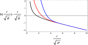
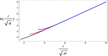
Figure 1: Evolution of $b(\frac{r}{\sqrt{\theta}})-(\frac{r}{\sqrt{\theta}})$ and $b(\frac{r}{\sqrt{\theta}})$ versus $\frac{r}{\sqrt{\theta}}$ for different values of $\frac{M}{\sqrt{\theta}}$. Herein for Gaussian distribution, $\frac{M}{\sqrt{\theta}}=0.2$ represents the black curve, $\frac{M}{\sqrt{\theta}}=2$ represents the red curve and $\frac{M}{\sqrt{\theta}}=10$ represents the blue curve.

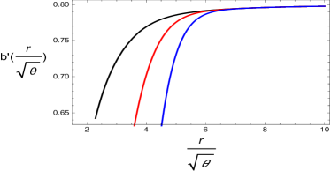
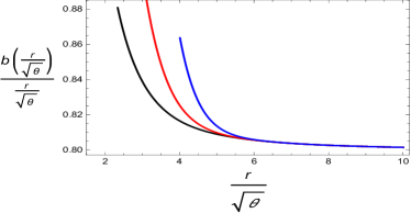
Figure 2: This indicates the behavior of $b^{\prime}(\frac{r}{\sqrt{\theta}})$ $\frac{b(\frac{r}{\sqrt{\theta}})}{\frac{r}{\sqrt{\theta}}}$ and versus $\frac{r}{\sqrt{\theta}}$ for different values of $\frac{M}{\sqrt{\theta}}$ in the framework of Gaussian distribution.

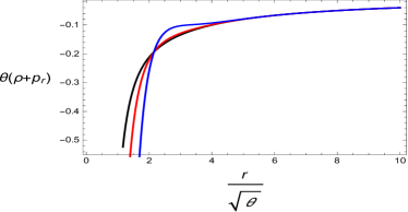
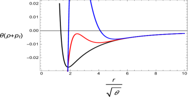
Figure 3: This shows the development of $\theta(\rho+p_{r})$ and $\theta(\rho+p_{t})$ versus $\frac{r}{\sqrt{\theta}}$ for different values of $\frac{M}{\sqrt{\theta}}$ in the framework of Gaussian distribution.

Now we will discuss some interesting aspects of the obtained shape function $b(r)$ which are considered as essential criteria for wormholes existence. For this purpose, we choose some suitable values of different free parameters involved. It is obvious that Eq.(24) depends on the coupling parameter $\lambda$, first we need to fix this parameter in order to analyze the results more comprehensively. Herein, we set $\lambda=2$ and represent the shape function $b(r)$ of the form $b(\frac{r}{\sqrt{\theta}})$ which depends on $\frac{M}{\sqrt{\theta}}$, dimensionless constant $C_{2}$ and integration constant $D_{1}$. One can choose $D_{1}=0$ as suggested in previous studies rahamanPLB , however in our case pick the suitable value of $D_{1}$ depending on $\lambda$. For Gaussian distributed non-commutative framework, we set $C_{2}=2$ and $D_{1}=-2\sqrt[-5]{\theta}$. The throat of wormhole is located at $\frac{r}{\sqrt{\theta}}=\frac{r_{0}}{\sqrt{\theta}}$, where $b(\frac{r}{\sqrt{\theta}})=\frac{r_{0}}{\sqrt{\theta}}$. For $\frac{M}{\sqrt{\theta}}=0.2$ (black curve), the throat of wormhole is located at $\frac{r_{0}}{\sqrt{\theta}}=1.678$, whereas for the other two values $\frac{M}{\sqrt{\theta}}=2$ (red curve) and $\frac{M}{\sqrt{\theta}}=10$ (blue curve), $b(\frac{r}{\sqrt{\theta}})-(\frac{r}{\sqrt{\theta}})$ crosses the horizontal axis at $\frac{r_{0}}{\sqrt{\theta}}=2.563$ and $\frac{r_{0}}{\sqrt{\theta}}=3.364$ respectively. It is noted that position of the throat is increasing with the increase of smeared mass distribution $M$ as shown in left plot of Figure 1. Right plot in Figure 1 shows that shape function has increasing behavior for Gaussian distribution for different values of $\frac{M}{\sqrt{\theta}}$. Validity of flaring out condition $b^{{}^{\prime}}(\frac{r}{\sqrt{\theta}})<1$ for $\frac{r}{\sqrt{\theta}}>\frac{r_{0}}{\sqrt{\theta}}$ is evident from left plot of Figure 2. Right plot in Figure 2 indicates that $\frac{b(\frac{r}{\sqrt{\theta}})}{\frac{r}{\sqrt{\theta}}}<1$ for $(\frac{r}{\sqrt{\theta}})>(\frac{r_{0}}{\sqrt{\theta}})$, which is an essential requirement for a shape function. We find that $\frac{b(\frac{r}{\sqrt{\theta}})}{\frac{r}{\sqrt{\theta}}}\rightarrow 4/5$ as $\frac{r}{\sqrt{\theta}}\rightarrow\infty$ as presented in Figure 2. In Figure 3, we presented the graphical behavior of the null energy conditions $\theta(\rho+p_{r})$ and $\theta(\rho+p_{t})$. It can be seen that NEC is violated so that the existence of wormholes requires exotic matter.

IV.2 Wormhole Existence with Lorentzian Distribution

Here we discuss the case of noncommutative geometry with the reference of Lorentzian distribution. In Lorentzian distribution, we take density function given by Eq.(2). Comparing Eqs.(2) and (14), we get

$$\frac{-2C_{2}^{2}(\lambda-1)+(6\lambda-2)\psi^{2}(r)+2(3\lambda-2)r\psi(r)\psi^{\prime}(r)}{2C_{2}^{2}\left(2\lambda^{2}+1\right)r^{2}}=\frac{M\sqrt{\theta}}{\pi^{2}(r^{2}+\theta)^{2}}.$$ (25)

Solving this differential equation, we get the value $\psi^{2}(r)$ as follows

$$\psi^{2}(r) = \frac{C_{2}^{2}r^{\frac{3\lambda}{3\lambda-2}+\frac{2-6\lambda}{3\lambda-2}+1}}{\pi^{2}\sqrt{\theta}(3\lambda-1)}\Bigg{[}\pi^{2}\sqrt{\theta}(\lambda-1)+\left(2\lambda^{2}M+M\right)\times\,_{2}F_{1}\left(1,\frac{1-3\lambda}{2-3\lambda};\frac{3-6\lambda}{2-3\lambda};-\frac{r^{2}}{\theta}\right)-\left(2\lambda^{2}M+M\right)$$ (26)

$$\times \,{}_{2}F_{1}\left(2,\frac{1-3\lambda}{2-3\lambda};\frac{3-6\lambda}{2-3\lambda};-\frac{r^{2}}{\theta}\right)\Bigg{]}+D_{2}r^{\frac{2-6\lambda}{3\lambda-2}},$$

where $D_{2}$ is an integration constants and ${}_{2}F_{1}$ is a hypergeometric function which is defined by

$${}_{2}F_{1}(a,b,c,z)=\sum^{\infty}_{n=0}\frac{(a)_{n}(b)_{n}}{c_{n}}\frac{t^{n}}{n!}.$$

Using this value of $\psi^{2}(r)$ in Eqs.(15) and (16), we get the exact values of radial and tangential pressures given by

$$p_{r} = \frac{1}{\lambda+1}\Bigg{[}\frac{6D_{2}(\lambda-1)r^{\frac{2}{2-3\lambda}-4}}{C_{2}^{2}(3\lambda-2)}+\frac{6(\lambda-1)\left(2\lambda^{2}+1\right)M\Gamma\left(\frac{1}{3\lambda-2}\right)}{\pi^{2}\sqrt{\theta}(3\lambda-2)^{3}r^{2}}+\frac{\sqrt{\theta}\lambda(\lambda+5)M}{\pi^{2}(3\lambda-2)\left(\theta+r^{2}\right)^{2}}-\frac{2(\lambda+1)}{(3\lambda-1)r^{2}}$$ (27)

$$\times \left(\,{}_{2}\tilde{F}_{1}\left(1,1+\frac{1}{3\lambda-2};2+\frac{1}{3\lambda-2};-\frac{r^{2}}{\theta}\right)-\,_{2}\tilde{F}_{1}\left(2,1+\frac{1}{3\lambda-2};2+\frac{1}{3\lambda-2};-\frac{r^{2}}{\theta}\right)\right)\Bigg{]},$$

$$p_{t} = \frac{1}{\pi^{2}(2-3\lambda)^{2}(\lambda+1)r^{4}}\Bigg{[}\frac{1}{C_{2}^{2}(3\lambda-1)\left(\theta+r^{2}\right)^{2}}\left(C_{2}^{2}r^{2}\left(\sqrt{\theta}(3\lambda-1)M\left(6\theta\lambda\left(2\lambda^{2}+1\right)+(\lambda(\lambda(27\lambda+5)+2)-4)r^{2}\right)\right.\right.$$ (28)

$$\left.\left.\pi^{2}(2-3\lambda)^{2}(\lambda+1)\left(\theta+r^{2}\right)^{2}\right)-6\pi^{2}D_{2}\lambda(9(\lambda-1)\lambda+2)\left(\theta+r^{2}\right)^{2}r^{\frac{2}{2-3\lambda}}\right)$$

$$- \frac{6\lambda\left(2\lambda^{2}+1\right)Mr^{2}\,_{2}F_{1}\left(1,1+\frac{1}{3\lambda-2};2+\frac{1}{3\lambda-2};-\frac{r^{2}}{\theta}\right)}{\sqrt{\theta}}\Bigg{]},$$

where ${}_{2}\tilde{F}_{1}$ is a regularized hypergeometric function which is defined as

$${}_{2}\tilde{F}_{1}=\sum^{\infty}_{n=0}\frac{(a)_{n}(b)_{n}}{\Gamma c_{n}}\frac{t^{n}}{n!}.$$

One can calculate the shape function $b(r)$ for Lorentizian distribution as follows

$$b(r) = \frac{-r}{\pi^{2}C_{2}^{2}\sqrt{\theta}(3\lambda-1)r}\left.\pi^{2}\sqrt{\theta}\left({C_{2}}^{2}(\lambda-1)r+D_{2}(3\lambda-1)r^{\frac{3\lambda}{2-3\lambda}}\right)\right.$$ (29)

$$+ \left.a^{2}\left(2\lambda^{2}+1\right)Mr\left(\,{}_{2}F_{1}\left(1,1+\frac{1}{3\lambda-2};2+\frac{1}{3\lambda-2};-\frac{r^{2}}{\theta}\right)\right.\right.$$

$$- \left.\left.\,{}_{2}F_{1}\left(2,1+\frac{1}{3\lambda-2};2+\frac{1}{3\lambda-2};-\frac{r^{2}}{\theta}\right)\right)\right)+r.$$

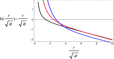
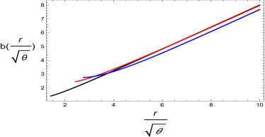
Figure 4: Evolution of $b(\frac{r}{\sqrt{\theta}})-(\frac{r}{\sqrt{\theta}})$ and $b(\frac{r}{\sqrt{\theta}})$ versus $\frac{r}{\sqrt{\theta}}$ for different values of $\frac{M}{\sqrt{\theta}}$. Herein for Lorentzian distribution, $\frac{M}{\sqrt{\theta}}=0.2$ represents the black curve, $\frac{M}{\sqrt{\theta}}=2$ represents the red curve and $\frac{M}{\sqrt{\theta}}=10$ represents the blue curve.

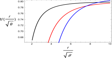
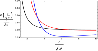
Figure 5: This indicates the behavior of $b^{\prime}(\frac{r}{\sqrt{\theta}})$ and $\frac{b(\frac{r}{\sqrt{\theta}})}{\frac{r}{\sqrt{\theta}}}$ versus $\frac{r}{\sqrt{\theta}}$ for different values of $\frac{M}{\sqrt{\theta}}$ in the framework of Lorentzian distribution.

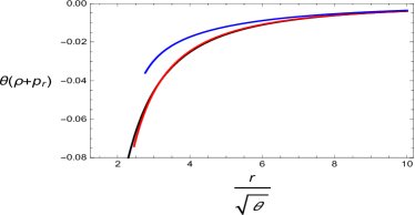
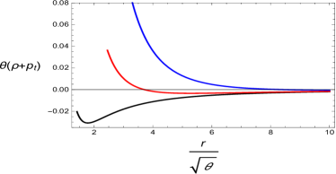
Figure 6: This shows the development of $\theta(\rho+p_{r})$ and $\theta(\rho+p_{t})$ versus $\frac{r}{\sqrt{\theta}}$ for different values of $\frac{M}{\sqrt{\theta}}$ in the framework of Lorentzian distribution.

Here, we discuss some properties of shape function $b(r)$ in the background of non-commutative Lorentzian distribution. It can be seen that Eq.(29) depends on mass $M$, $\theta$ (the non-commutative parameter) and the coupling parameter $\lambda$. Initially, we select the particular value for the coupling parameter $\lambda$ and analyze the results depending on the choice of other parameters. Herein, we set $\lambda=2$ and represent the shape function $b(r)$ of the form $b(\frac{r}{\sqrt{\theta}})$ which depends on $\frac{M}{\sqrt{\theta}}$, dimensionless constant $C_{2}$ and integration constant $D_{2}$. $D_{2}$ can be selected as null rahamanPLB , however in this case, we pick the suitable value of $D_{2}$ depending on the choice $\lambda$. For Lorentzian distributed non-commutative framework, we set $C_{2}=2$. The throat of wormhole is located at $\frac{r}{\sqrt{\theta}}=\frac{r_{0}}{\sqrt{\theta}}$, where $b(\frac{r}{\sqrt{\theta}})=\frac{r_{0}}{\sqrt{\theta}}$. We explore the evolution of shape function depending on the choice of $\frac{M}{\sqrt{\theta}}$. In left plot of Figure 4, we present the evolution of $b(\frac{r}{\sqrt{\theta}})$ versus $\frac{r}{\sqrt{\theta}}$, it can be seen that for $\frac{M}{\sqrt{\theta}}=0.2$ (black curve) with $D_{2}=-2\sqrt[-5]{\theta}$, the throat of wormhole is located at $\frac{r_{0}}{\sqrt{\theta}}=1.42$. For $\frac{M}{\sqrt{\theta}}=2$ (red curve) with $D_{2}=-10\sqrt[-5]{\theta}$, the location of throat is at $\frac{r_{0}}{\sqrt{\theta}}=2.45$ whereas for $\frac{M}{\sqrt{\theta}}=10$ (blue curve) with $D_{2}=-25\sqrt[-5]{\theta}$, $b(\frac{r}{\sqrt{\theta}})-(\frac{r}{\sqrt{\theta}})$ crosses the horizontal axis at $\frac{r_{0}}{\sqrt{\theta}}=2.76$. It is deduced that position of throat increases depending on the choice of smeared mass distribution $M$ in similar fashion as in in Gaussian distribution. We also present the evolution of $b(\frac{r}{\sqrt{\theta}})$ on the right side of Figure 4 for different values of $\frac{M}{\sqrt{\theta}}$. Left plot of Figure 5 presents the evolution of flaring out condition which interprets $b^{{}^{\prime}}(\frac{r}{\sqrt{\theta}})<1$ for $\frac{r}{\sqrt{\theta}}>\frac{r_{0}}{\sqrt{\theta}}$ in all the cases. We also evaluate $\frac{b(\frac{r}{\sqrt{\theta}})}{\frac{r}{\sqrt{\theta}}}$ in the limit of $\frac{r}{\sqrt{\theta}}\rightarrow\infty$, it is found that $\frac{b(\frac{r}{\sqrt{\theta}})}{\frac{r}{\sqrt{\theta}}}\rightarrow 4/5$ similar to the previous Gaussian distribution case. The dynamical behavior of null energy conditions $\theta(\rho+p_{r})$ and $\theta(\rho+p_{t})$ is shown in Figure 6 and show similar evolution as in Gaussian distribution.

V Equilibrium Condition

In this segment, we explore the stability of obtained wormhole solutions for both non-commutative distributions using equilibrium condition. For this purpose, we take Tolman-Oppenheimer-Volkov equation which is given by

$$\frac{dp_{r}}{dr}+\frac{\sigma^{{}^{\prime}}}{2}(\rho+p_{r})+\frac{2}{r}(p_{r}-p_{t})=0,$$ (30)

where $\sigma(r)=2\Phi(r)$. This equation determines the equilibrium state of configuration by taking the gravitational, hydrostatic as well as the anisotropic forces (arising due to anisotropy of matter) into account. These forces are defined by the following relations:

$$F_{g}=-\frac{\sigma^{{}^{\prime}}(\rho+p_{r})}{2},\;\;\;\;\;\;\;\;F_{h}=-\frac{dp_{r}}{dr},\;\;\;\;\;\;\;\;F_{a}=2\frac{(p_{t}-p_{r})}{r},$$

and thus Eq.(30) takes the form given by

$$F_{a}+F_{g}+F_{h}=0.$$ (31)

Firstly, we calculate these forces $F_{g}$, $F_{h}$ and $F_{a}$ for Gaussian distribution as follows

$$F_{g} = -\frac{1}{8\pi^{3/2}\theta^{3/2}r}\Bigg{[}\frac{e^{-\frac{r^{2}}{4\theta}}}{C_{2}^{2}\left(9\lambda^{3}-7\lambda+2\right)r^{4}}\bigg{[}2C_{2}^{2}r^{2}\bigg{[}(\lambda(\lambda(6\lambda+7)-6)+1)Mr^{2}-8\pi^{3/2}\theta^{3/2}\left(3\lambda^{2}+\lambda-2\right)e^{\frac{r^{2}}{4\theta}}\bigg{]}$$

$$+ 48\pi^{3/2}D_{1}\theta^{3/2}(\lambda-1)(3\lambda-1)e^{\frac{r^{2}}{4\theta}}r^{\frac{2}{2-3\lambda}}\bigg{]}-\frac{6(\lambda-1)\left(2\lambda^{2}+1\right)ME_{\frac{1}{2-3\lambda}-1}\left(\frac{r^{2}}{4\theta}\right)}{(2-3\lambda)^{2}(\lambda+1)}\Bigg{]},$$

$$F_{h} = -\frac{1}{8(\lambda+1)}\Bigg{[}-\frac{288D_{1}(\lambda-1)(2\lambda-1)r^{\frac{2}{2-3\lambda}-5}}{C_{2}^{2}(2-3\lambda)^{2}}+\frac{3(\lambda-1)\left(2\lambda^{2}+1\right)MrE_{\frac{1}{2-3\lambda}-2}\left(\frac{r^{2}}{4\theta}\right)}{\pi^{3/2}\theta^{5/2}(2-3\lambda)^{2}}-\frac{\lambda(\lambda+5)Mre^{-\frac{r^{2}}{4\theta}}}{2\pi^{3/2}\theta^{5/2}(3\lambda-2)}$$

$$+ \frac{16(\lambda(3\lambda+2)+1)}{\left(2\lambda^{2}+1\right)r^{3}}+\frac{16\left(-5\lambda^{3}+\lambda^{2}+\lambda+3\right)}{(3\lambda-1)\left(2\lambda^{2}+1\right)r^{3}}\Bigg{]},$$

$$F_{a} = \frac{1}{2\pi^{3/2}C_{2}^{2}\theta^{3/2}(2-3\lambda)^{2}(\lambda+1)(3\lambda-1)r^{5}}\Bigg{[}e^{-\frac{r^{2}}{4\theta}}\left((3\lambda-2)\left(C_{2}^{2}r^{2}\left((3\lambda-1)\left(2\lambda^{2}+1\right)Mr^{2}+4\pi^{3/2}\theta^{3/2}(\lambda+1)\right.\right.\right.$$

$$\times \left.\left.\left.(3\lambda-2)e^{\frac{r^{2}}{4\theta}}\right)-24\pi^{3/2}D_{1}\theta^{3/2}(\lambda(6\lambda-5)+1)e^{\frac{r^{2}}{4\theta}}r^{\frac{2}{2-3\lambda}}\right)+3C_{2}^{2}(2\lambda-1)(3\lambda-1)\left(2\lambda^{2}+1\right)Mr^{4}e^{\frac{r^{2}}{4\theta}}E_{\frac{1}{2-3\lambda}-1}\left(\frac{r^{2}}{4\theta}\right)\right)\Bigg{]}.$$

In case of Lorentizian distribution of non-commutative geometry, these forces are given by

$$F_{g} = \frac{2}{r^{5}}\bigg{[}-\frac{3D_{2}(\lambda-1)r^{\frac{2}{2-3\lambda}}}{C_{2}^{2}\left(3\lambda^{2}+\lambda-2\right)}+\frac{\sqrt{\theta}(1-\lambda(2\lambda+3))Mr^{4}}{\pi^{2}\left(3\lambda^{2}+\lambda-2\right)\left(\theta+r^{2}\right)^{2}}+\frac{r^{2}}{3\lambda-1}+\frac{3(\lambda-1)\left(2\lambda^{2}+1\right)Mr^{2}\Gamma\left(\frac{1}{3\lambda-2}\right)}{\pi^{2}\sqrt{\theta}(\lambda+1)(3\lambda-2)^{3}}$$

$$\times \bigg{[}\,_{2}\tilde{F}_{1}\left(2,1+\frac{1}{3\lambda-2};2+\frac{1}{3\lambda-2};-\frac{r^{2}}{\theta}\right)-\,_{2}\tilde{F}_{1}\left(1,1+\frac{1}{3\lambda-2};2+\frac{1}{3\lambda-2};-\frac{r^{2}}{\theta}\right)\bigg{]}\bigg{]},$$

$$F_{h} = \frac{4}{r^{5}}\bigg{[}\frac{r^{2}}{1-3\lambda}+\frac{9D_{2}(\lambda-1)(2\lambda-1)r^{\frac{2}{2-3\lambda}}}{C_{2}^{2}(2-3\lambda)^{2}(\lambda+1)}-\frac{3\sqrt{\theta}(\lambda-1)\left(2\lambda^{2}+1\right)Mr^{4}}{\pi^{2}(2-3\lambda)^{2}(\lambda+1)\left(\theta+r^{2}\right)^{2}}+\frac{\sqrt{\theta}\lambda(\lambda+5)Mr^{6}}{\pi^{2}\left(3\lambda^{2}+\lambda-2\right)\left(\theta+r^{2}\right)^{3}}$$

$$+ \frac{9(\lambda-1)(2\lambda-1)\left(2\lambda^{2}+1\right)Mr^{2}\Gamma\left(\frac{1}{3\lambda-2}\right)}{\pi^{2}\sqrt{\theta}(2-3\lambda)^{4}(\lambda+1)}\times\left(\,{}_{2}\tilde{F}_{1}\left(1,1+\frac{1}{3\lambda-2};2+\frac{1}{3\lambda-2};-\frac{r^{2}}{\theta}\right)\right.$$

$$- \left.\,{}_{2}\tilde{F}_{1}\left(2,1+\frac{1}{3\lambda-2};2+\frac{1}{3\lambda-2};-\frac{r^{2}}{\theta}\right)\right)\bigg{]},$$

$$F_{a} = \frac{2}{\pi^{2}(2-3\lambda)^{2}(\lambda+1)r^{5}}\Bigg{[}\frac{1}{C_{2}^{2}(3\lambda-1)\left(\theta+r^{2}\right)^{2}}\bigg{[}C_{2}^{2}r^{2}\bigg{[}2\sqrt{\theta}(3\lambda-1)\left(2\lambda^{2}+1\right)M\left(6\theta\lambda-3\theta+(9\lambda-5)r^{2}\right)$$

$$+ \pi^{2}(\lambda+1)(2-3\lambda)^{2}\left(\theta+r^{2}\right)^{2}\bigg{]}-6\pi^{2}D_{2}(2\lambda-1)(3\lambda-2)(3\lambda-1)\left(\theta+r^{2}\right)^{2}r^{\frac{2}{2-3\lambda}}\bigg{]}$$

$$- \frac{6(2\lambda-1)\left(2\lambda^{2}+1\right)Mr^{2}\,_{2}F_{1}\left(1,1+\frac{1}{3\lambda-2};2+\frac{1}{3\lambda-2};-\frac{r^{2}}{\theta}\right)}{\sqrt{\theta}}\Bigg{]}.$$

The graphical illustration of these forces is given in Figure 7. The left graph indicates the behavior of these forces for Gaussian distribution, while the right graph corresponds to Lorentzian distribution. It is evident from these graphs that the stability of configuration has been attained as gravitational and anisotropic forces show opposite behavior to hydrostatic force and hence cancel each other’s effect.

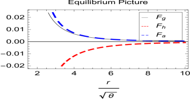
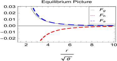
Figure 7: This shows the graphical illustration of $F_{a}$, $F_{g}$ and $F_{h}$ forces versus $r$ for Gaussian and Lorentizian distribution, in the left and right panels, respectively. In left plot we set $\frac{M}{\sqrt{\theta}}=0.2$ and $\frac{r_{0}}{\sqrt{\theta}}=1.678$, whereas in right plot the selected parameters are $\frac{M}{\sqrt{\theta}}=0.2$ and $\frac{r_{0}}{\sqrt{\theta}}=1.420$.

VI Active Gravitational Mass

The active gravitational mass within the region from the throat $r_{0}$ up to the radius $R$ can be found by using the relation $M_{active}=4\pi\int_{\text{r0}}^{R}\rho r^{2}\,dr$. For Gaussian distribution, it is given by

$$M_{active}=M\left[\text{erf}\left(\frac{r}{2\sqrt{\theta}}\right)-\frac{re^{-\frac{r^{2}}{4\theta}}}{\sqrt{\pi}\sqrt{\theta}}\right]^{R}_{r_{0}}.$$ (32)

In case of Lorentizian distribution, we have

$$M_{active}=\frac{2M}{\pi}\left[\tan^{-1}\left(\frac{r}{\sqrt{\theta}}\right)-\frac{\sqrt{\theta}r}{\theta+r^{2}}\right]^{R}_{r_{0}}.$$ (33)

We observe that by above equation the active gravitational mass $M_{active}$ of the wormhole is positive under the constraint $\text{erf}\left(\frac{r}{2\sqrt{\theta}}\right)>\frac{re^{-\frac{r^{2}}{4\theta}}}{\sqrt{\pi}\sqrt{\theta}}$ for Gaussian distribuion and $\tan^{-1}\left(\frac{r}{\sqrt{\theta}}\right)>\frac{\sqrt{\theta}r}{\theta+r^{2}}$ for Lorentizian distribution. The physical nature of active gravitational mass can be seen from Figure 8.

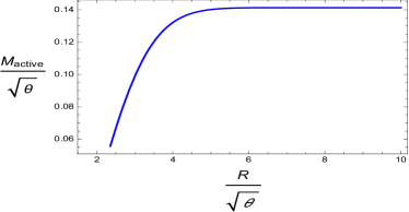
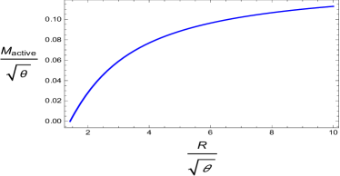
Figure 8: This shows the graphical illustration of $\frac{M_{active}}{\sqrt{\theta}}$ versus $\frac{R}{\sqrt{\theta}}$ for Gaussian and Lorentizian distributions, in the left and right panels, respectively. In left plot we set $\frac{M}{\sqrt{\theta}}=0.2$ and $\frac{r_{0}}{\sqrt{\theta}}=1.678$, whereas in right plot the selected parameters are $\frac{M}{\sqrt{\theta}}=0.2$ and $\frac{r_{0}}{\sqrt{\theta}}=1.420$.

VII Conclusion

In the present manuscript, we have explored the existence of spherically symmetric wormhole solutions by taking corresponding CKVs into account. For this purpose, we consider anisotropic matter contents along with Gaussian and Lorentzian distributions of non-commutative geometry. The concept of introducing CKVs and non-commutative distributions for finding solutions is not a new approach. These concepts have already been used in literature in various contexts like in investigating the existence of wormholes and black holes in different gravitational theories. However, the present work provides a unique discussion in the sense that such approach of conformal motion along with non-commutative distribution has not been used before in $f(R,T)$ theory. In this respect, Kuhfittig 1* has used non-commutative geometry in $f(R)$ gravity to discuss different forms of $f(R)$ function by taking different choices of shape functions into account. In 2* , the same author introduced CKVs to check the existence and stability of wormholes by using phantom energy, i.e., $p=\omega\rho;~{}\omega<-1$. Jamil et al. 3* discussed the wormhole solutions by considering non-commutative geometry in $f(R)$ gravity. In another study 4* , non-commutative distributions are used to reconstruct $f(R)$ models by taking two choices of shape function. In 5* , Singh et al. have introduced the aspects of non-commutative geometry to discuss the rotating black string where they also examined the stability by checking thermodynamical properties of solutions. In another study, Ghosh et al. Ghosh introduced non-commutative geometry to discuss the existence of Einstein-Gauss-Bonnet black hole. Nicolini et al. 6** investigated the behavior of a noncommutative radiating Schwarzschild black hole. In our recent paper 10 , we have also introduced the concept of non-commutativity in $f(R,T)$ gravity (without including CKVs) to check the possible existence and stability of wormhole solutions. It is seen that due to complex form of resulting field equations, we discussed wormhole solutions numerically there except for few cases.

In the present paper, for both non-commutative distributions, the use of CKVs simplifies the resulting field equations and consequently leads to the analytical solutions of field equations which meet all the necessary criteria for wormhole existence. We have shown these properties of wormholes graphically. We have firstly defined the possible CKVs of a general static spherically symmetric spacetime which leads to simplicity in calculations further. With the help of these CKVs, we have formulated a relatively simplified form of field equations. By considering the density functions of Gaussian and Lorentzian distributions of non-commutative geometry, it is seen that the conformal killing vector $\psi(r)$ is obtained in terms of exponential and hypergeometric functions of mathematics. By using these CKVs, we have explored the corresponding forms of shape functions and their behavior graphically as shown in Figures 1-8. By fixing the arbitrary constants, graphical analysis has been done in terms of dimension less variable, i.e., we plotted all the properties of shape function versus $\frac{r}{\sqrt{\theta}}$ for three different choices of $\frac{M}{\sqrt{\theta}}$. The obtained results can be summarized as follows:

• the obtained shape functions, in both cases, are increasing functions in nature versus $\frac{r}{\sqrt{\theta}}$.

• the validity of flaring out property has been achieved in both cases.

• for the constructed shape functions, in both cases, $\frac{b(\frac{r}{\sqrt{\theta}})}{\frac{r}{\sqrt{\theta}}}$ approaches to a constant value of $\frac{4}{5}$ as $\frac{r}{\sqrt{\theta}}\rightarrow\infty$.

• it is seen that the values of wormhole throat increase as the values of $\frac{M}{\sqrt{\theta}}$ increase in both Gaussian and Lorentzian distributions.

• At these wormhole throats, it has been shown graphically that the condition $b^{\prime}(\frac{r_{0}}{\sqrt{\theta}})<1$ holds in both cases.

• the NEC bounds are violated and thus confirming the presence of exotic matter that is a basic requirement for wormhole existence.

• using Tolman-Oppenheimer-Volkov equilibrium condition, it is seen from the graphical behavior of gravitational, hydrostatic and anisotropic forces, the obtained wormhole solutions are stable. Basically these forces balance each other’s effect and hence leave a stable configuration.

• the forms of active gravitational mass show positive increasing behavior under some certain constraints imposed on the free parameters in both cases.

It would be interesting to explore the existence of wormhole solutions using CKVs in other modified gravity theories.

References

• (1) Bento, M.C., Bertolami, O. and Sen, A.A.: Phys. Rev. D 66(2002)043507; Fujii, Y.: Phys. Rev. D 26(1982)2580; Ford, L.H.: Phys. Rev. D 35(1987)2339; Wetterich, C.: Nucl. Phys. B 302(1988)668; Ratra, B. and Peebles, P.J.E.: Phys. Rev. D 37(1988)3406; Chiba, T., Sugiyama, N. and Nakamura, T.: Mon. Not. Roy. Astron. Soc. 289(1997)L5; Caldwell, R.R., Dave, R. and Steinhardt, P.J.: Phys. Rev. Lett. 80(1998)1582; Armendariz-Picon, C., Damour, T. and Mukhanov, V.F.: Phys. Lett. B 458(1999)209; Chiba, T., Okabe, T. and Yamaguchi, M.: Phys. Rev. D 62(2000)023511, Chimento, L.P.: Phys. Rev. D 69(2004)123517; Chimento, L.P. and Feinstein, A.: Mod. Phys. Lett. A 19(2004)761.
• (2) Nojiri, S. and Oditsov, S.D.: Phys. Rep. 505(2011)59; Starobinksy, A. A.: Phys. Lett. B 91(1980)99; Ferraro, R. and Fiorini, F.: Phys. Rev. D 75(2007)084031; Zubair, M.: Int. J. Modern. Phys. D 25(2016)1650057; Carroll, S. et al., Phys. Rev. D 71, 063513 (2005); Cognola, G.: Phys. Rev. D 73(2006)084007; Agnese, A. G. and Camera, M. La.: Phys. Rev. D 51(1995)2011; Kofinas, G. and Saridakis, N. E.: Phys. Rev. D 90(2014)084044; Sharif, M. and Waheed, S.: Adv. High Energy Phys. 2013(2013)253985.
• (3) Harko, T. et al.: Phys. Rev. D 84(2011)024020.
• (4) Houndjo, M. J. S. et al.: Int. J. Mod. Phys. D 21(2012)1250003.
• (5) Houndjo, M. J. S. et al.: Int. J. Mod. Phys. 2(2012)1250024.
• (6) Sharif, M. and Zubair, M.: JCAP 03(2012)028.
• (7) Singh, C.P. and Singh, V.: Gen. Relativ. Gravitt. 46(2014)1696; Mubasher et al.: Eur. Phys. J. C 72(2012)1999; Sharif, M. and Zubair, M.: J. Phys. Soc. Jpn. 82(2013)064001; Shabani, H. and Farhoudi, M.: Phys. Rev. D 88(2013)044048; ibid. Phys. Rev. D 90(2014)044031; Santos, A.F.: Modern Phys. Lett. A 28(2013)1350141; M. Sharif, M. Zubair, Gen. Relativ. Gravit. 46(2014)1723; Zubair, M. and Noureen, I.: Eur. Phys. J. C 75(2015)265; Noureen, I. and Zubair, M.: Eur. Phys. J. C 75(2015)62; Noureen, I. and Zubair, M., Bhatti, A.A. and Abbas, G.: Eur. Phys. J. C 75(2015)323; Alvarenga et al.: Phys. Rev. D 87(2013)103526; Baffou et al. Astrophys. Space Sci. 356(2015)173; Shamir, M.F.: Eur. Phys. J. C 75(2015)354; Moraes, P.H.R.S.: Eur. Phys. J. C 75(2015)168; Zubair, M. et al.: Astrophys Space Sci. 361(2016)8; Zubair, M. and Syed M. Ali Hassan.: Astrophys Space Sci. 361(2016)149; Shahbani, H.: arXiv:1604.04616v1.
• (8) Einstein, A. and Rosen, N.: Phys. Rev. 48(1935)73.
• (9) Morris, M. S. and Thorne, K. S.: Am. J. Phys. 56(1988)395.
• (10) M. Zubair, G. Mustafa, Saira Waheed and G. Abbas, Eur. Phys. J C 77(2017)680.
• (11) Zubair, M., Waheed, S. and Ahmad, Y.: Eur. Phys. J C 76(2016)8.
• (12) Kim, S. W. and Lee, H.: Phys. Rev. D 63(2001)064014; Jamil, M. and Farooq, M. U.: Int. J. Theor. Phys. 49(2010)835; Rahaman, F. and Islam, S., Kuhfittig, P. K. F. and Ray, S.: Phys. Rev. D 86(2012)106010; Lobo, F.S.N., Parsaei, F. and Riazi, N.: Phys. Rev. D 87(2013)084030; Rahaman, F. et al.: Int. J. Theor. Phys. 53(2014)1910; Sharif, M. and Rani, S.: Eur. Phy. J. Plus 129(2014)237; Jamil, M. et al.: J. Korean Phys. Soc. 65(2014)917; Khufittig, P. K. F.: Eur. Phys. J. C 74(2014)2818.
• (13) Witten, E.: Nucl. Phys. B 460(1996)335; Seiberg, N. and Witten, E.: J. High Energy Phys. 09 (1999).
• (14) Gruppuso, A.: J. Phys. A 38(2005)2039; Smailagic, A. and Spalluci, E. : J. Phys. A 36(2003)467L; Nicolini, P., Smailagic, A. and Spalluci, E.: Phys. Lett. B 632(2006)547.
• (15) Sushkov, S. V.: Phys. Rev. D 71(2005)043520.
• (16) Nicolini, P. and Spalluci, E.: Classical Quantum Gravity 27(2010)015010.
• (17) Ghosh, S.G.: Class. Quantum Grav. 35(2018)085008.
• (18) Nicolini, P. et al.: Phys. Lett. B 632 (2006) 547 551.
• (19) F. Rahaman, et al. Phys. Lett. B 746(2015)73 78.
• (20) Khufittig, P. K. F.: Eur. Phys. J. C 74(2014)2818.
• (21) Kuhfittig, P.K.F.: Indian J. Phys. 92(2018)1207.
• (22) Kuhfittig, P.K.F.: Int. J. Mod. Phys. D 26(2017)1750025.
• (23) Jamil, M., Rahaman, F. and Myrzakulov, R.: J. Korean. Phys. Soci. 65(2014)917.
• (24) Rahaman et al.: Int. J. Theor. Phys. 53(2014)1910.
• (25) Singh, D.V., Ali, S.M. and Ghosh, S.G.: Int. J. Mod. Phys . D 27(2018)1850108.