Machine learning a model for RNA structure prediction

Abstract

RNA function crucially depends on its structure. Thermodynamic models currently used for secondary structure prediction rely on computing the partition function of folding ensembles, and can thus estimate minimum free-energy structures and ensemble populations. These models sometimes fail in identifying native structures unless complemented by auxiliary experimental data. Here, we build a set of models that combine thermodynamic parameters, chemical probing data (DMS, SHAPE), and co-evolutionary data (Direct Coupling Analysis, DCA) through a network that outputs perturbations to the ensemble free energy. Perturbations are trained to increase the ensemble populations of a representative set of known native RNA structures. In the chemical probing nodes of the network, a convolutional window combines neighboring reactivities, enlightening their structural information content and the contribution of local conformational ensembles. Regularization is used to limit overfitting and improve transferability. The most transferable model is selected through a cross-validation strategy that estimates the performance of models on systems on which they are not trained. With the selected model we obtain increased ensemble populations for native structures and more accurate predictions in an independent validation set. The flexibility of the approach allows the model to be easily retrained and adapted to incorporate arbitrary experimental information.

1 Introduction

Ribonucleic acids (RNA) transcripts, and in particular non-coding RNAs, play a fundamental role in cellular metabolism being involved in protein synthesis [1], catalysis [2], and regulation of gene expression [3]. RNAs often adopt dynamic interconverting conformations, to regulate their functional activity. Their function is however largely dependent on a specific active conformation [4], making RNA structure determination fundamental to identify the role of transcripts and the relationships between mutations and diseases [5]. The nearest-neighbor models based on thermodynamic parameters [6, 22] allow the stability of a given RNA secondary structure to be predicted with high reliability, and dynamic programming algorithms [8, 9] can be used to quickly identify the most stable structure or the entire partition function for a given RNA sequence. However, the coexistence of a large number of structures in a narrow energetic range [10] often makes the interpretation of the results difficult. Whereas there are important cases where multiple structures are indeed expected to coexist in vivo and might be necessary for function [11, 12], the correct identification of the dominant structure(s) is crucial to elucidate RNA function and mechanism of action. In order to compensate for the inaccuracy of thermodynamic models, it is becoming common to complement them with chemical probing data [13] providing nucleotide-resolution information that can be used to infer pairing propensities (e.g., reactive nucleotides are usually unpaired). Particularly interesting is selective 2^′ hydroxyl acylation analyzed via primer extension (SHAPE) [14, 15], as it can also probe RNA structure in vivo [16]. In a separate direction, novel methodologies based on direct coupling analysis (DCA) have been developed to optimally exploit co-evolutionary information in protein structure prediction [17] and found their way in the RNA world as well [18, 19]. Whereas the use of chemical probing data and of multiple sequence alignments in RNA structure prediction is becoming more and more common, these two types of information have been rarely combined [20].

In this paper, we propose a model to optimally integrate RNA thermodynamic models, chemical probing experiments, and DCA co-evolutionary information into a robust structure prediction protocol. A machine learning procedure is then used to select the appropriate model and optimize the model parameters based on available experimental structures. Regularization hyperparameters are used to tune the complexity of the model thus controlling overfitting and enhancing transferability. The resulting model leads to secondary structure prediction that surpasses available methods when used on a validation set not seen in the training phase. The parameters can be straightforwardly re-trained on new available data.

2 MATERIALS AND METHODS

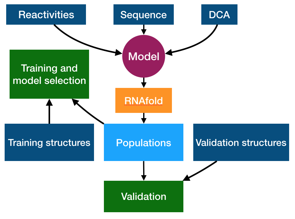
(a)

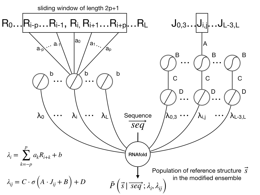
(b)

Figure 1: Graphical scheme of the machine learning procedure. (a) Models that integrate RNAfold, chemical probing experiments, and DCA scores into prediction of structure populations are trained. One among all the proposed models is selected based on a transferability criterion and validated against data that is not seen during training. Available reference structures are used as target for training and validation. (b) Sequence, reactivity profile, and DCA data are included through additional terms in the RNAfold model free energy. The network is split into two channels: a single-layered channel for reactivity input (left side) and a double-layered channel for DCA couplings (right side). Along the reactivity channel, a convolutional layer operates a linear combination on the sliding window including the reactivity $R_{i}$ of a nucleotide and the reactivities $\{R_{i+k}\}$ of its neighbors, with weights $\{a_{k}\}$ and bias $b$. The output consists in a pairing penalty $\lambda_{i}$ for the $i$-th nucleotide. In the DCA channel, the first layer transforms the input DCA coupling $J_{ij}$ via a non-linear (sigmoid) activation function, with weight $A$ and bias $B$. The transformed DCA input is then mapped to a pairing penalty $\lambda_{ij}$ for the specific $ij$ pair via a second layer, implementing a linear activation function with weight $C$ and bias $D$. Penalties for both individual nucleotides and for specific pairs are applied as perturbations to the RNAfold free-energy model.

The architecture of the model is summarized in Fig. 1.

2.1 Secondary structure annotation

The secondary structures that we use for training and validation were obtained by annotating crystallographic structures with x3dna-dssr [21]. Differently from previous work, we include all the computed cis-Watson-Crick contacts as reference base pairs, with exception of pseudoknots that are forbidden in predictions made with RNAfold. All of the reference structures are published in the PDB database and have a resolution better than $4\text{\,}\mathrm{\SIUnitSymbolAngstrom}$ so that they can be assumed to be of similar quality, although crystal packing effects or other artefacts might in principle be different. The list of PDB files used in this work is reported in Table 1.

Molecule	PDB	$\textit{l}_{seq}$	S1–S4
yeast Phe-tRNA	1EHZ	76	VTTT
D5,6 Yeast ai5g G-II Intron	1KXK	70	TTTT
Ribonuclease P RNA	1NBS	150	TTTT
Adenine riboswitch	1Y26	71	VTTV
TPP riboswtich	2GDI	78	TTVT
SAM-I riboswitch	2GIS	94	TTVT
Lysine riboswitch	3DIG	174	TTVV
O. I. G-II Intron	3IGI	388	TVTV
c-di-GMP riboswitch	3IRW	90	TTTT
M-box riboswitch	3PDR	161	VVTT
THF riboswitch	3SD3	89	VVTT
Fluoride riboswitch	3VRS	52	VTTT
SAM-I/IV riboswitch	4L81	96	TVVV
Lariat capping ribozyme	4P8Z	188	TTTT
ydaO riboswitch	4QLM	108	TTTT
ZMP riboswitch	4XW7	64	VVVV
50S ribosomal	4YBB_CB	120	TVVV
5-HTP RNA aptamer	5KPY	71	TTTT

Table 1: RNA molecules included in the dataset. For each molecule we indicate the PDB ID of the corresponding annotated structure, the number of nucleotides ($\textit{l}_{seq}$), and, for each random dataset splitting that we used (S1 to S4), a mark to denote whether the molecule data are used for training (T) or validation (V). For PDB 4YBB, chain CB was used as a reference.

2.2 Thermodynamic model

As a starting point we use the nearest neighbor thermodynamic model [6, 22] as implemented using dynamic programming [8] in the ViennaRNA package [9]. Given a sequence $\vec{seq}$ the model estimates the free energy associated to any possible secondary structure $\vec{s}$ by means of a sum over consecutive base pairs, with parameters based on the identity of each involved nucleobase. We denote this free energy as $F_{0}\left(\vec{s}|\vec{seq}\right)$. We used here the thermodynamic parameters derived in [22] as implemented in the ViennaRNA package, but the method could be retrained starting with alternative parameters. The probability $P_{0}\left(\vec{s}|\vec{seq}\right)$ of a structure $\vec{s}$ to be observed is thus $P_{0}\left(\vec{s}|\vec{seq}\right)=e^{-\frac{1}{RT}F_{0}\left(\vec{s}|\vec{seq}\right)}/Z_{0}\left(\vec{seq}\right)$ where $Z_{0}$ is the partition function, $R$ is the gas constant and $T$ the temperature, here set to 300K. Importantly, the implemented algorithm is capable of finding not only the most stable structure associated to a sequence ($\text{arg min}_{\vec{s}}F_{0}\left(\vec{s}|\vec{seq}\right)$) but also the full partition function $Z_{0}$ and the probability of each base pair to be formed in a polynomial time frame [23].

2.3 Experimental data

2.3.1 Chemical probing data.

Reactivities for systems 1KXK, 2GIS, 3IRW, 3SD3, 3VRS and 4XW7 were collected for this work. Single stranded DNA templates containing the T7 promoter region and the 3’ and 5’ SHAPE cassettes [24] were ordered from Eurofins Genomics. RNAs were transcribed using in-house prepared T7 polymerase. Briefly, complementary T7 promoter DNA was mixed with the desired DNA template and snap cooled ($95\text{\,}\mathrm{\SIUnitSymbolCelsius}$ for 5 minutes, followed by incubation on ice for 10 minutes) to ensure annealing of the T7 complementary promoter with template DNA. The mixture was supplemented with rNTPs, 20X transcription buffer (TRIS pH $8$, $100\text{\,}\mathrm{mM}$ Spermidine, $200\text{\,}\mathrm{mM}$ DTT), PEG 8000, various concentrations of MgCl2 (final concentration ranging from $10$ to $40\text{\,}\mathrm{mM}$), and T7 ($10\text{\,}\mathrm{m}\mathrm{g}\mathrm{/}\mathrm{m}\mathrm{L}$). The RNAs were purified under denaturing conditions using polyacrylamide gel electrophoresis. RNA was excised from the gel and extracted using the crush and soak method [25]. Following crush and soak, the RNAs were precipitated using ethanol and sodium acetate, and resuspended in RNAse-free water. SHAPE modification followed by reverse transcription (using 5’ FAM labeled primers) was carried out as previously described [24]. Following reverse transcription, RNAs were precipitated using ethanol and sodium acetate, redissolved in HiDi formamide, and cDNA fragments separated using capillary electrophoresis (ABI 3130 Sequencer). Raw reads corresponding to cDNA fragments were obtained using QuSHAPE [26] and are reported in Supporting Information. Reads in each of the control and modifier channels were first normalized independently by dividing them by the sum of reads in the corresponding channel. Reactivities were then estimated by subtracting the normalized reads in the control channel from the normalized reads in the modifier channel, with negative values replaced with zeros. This normalization is a simplified version of the one proposed in Ref. [27] and does not contain position dependent corrections. Reactivities to different chemical probes, namely 1M7 for systems 1EHZ, 1NBS, 1Y26, 2GDI, 3DIG, 3IGI, 3PDR, 4L81, 4YBB_CB and 5KPY, NMIA for 1NBS, and DMS for 4P8Z and 4QLM, were taken from the literature [28, 29, 30, 31] and were normalized using the procedure discussed above, except where noted.

2.3.2 DCA data.

Direct couplings for all the systems were calculated using the same code and parameters reported in Ref. [32], but alignment was performed with ClustalW [33] to avoid including indirectly known structural information. For systems where the RNA primary sequences used in Ref. [32] were different from those reported in the PDB or used in chemical probing experiments, DCA calculations were performed again. Couplings $J_{ij}$ were computed as the Frobenius norm of the couplings between positions $i$ and $j$, as detailed in Ref. [32]. All the used alignments and couplings are reported in Supporting Information.

2.4 Penalties

We integrate chemical probing reactivities $R_{i}$ and direct couplings $J_{ij}$ into the model by mapping them into single-point penalties $\lambda_{i}$ and pairwise penalties $\lambda_{ij}$ to pairing propensity of, respectively, individual nucleotides and specific nucleotide pairs. The free energy estimate $F\left(\vec{s}|\vec{seq};\vec{R},\vec{J}\right)$ obtained in this way is a modification of the original one by two additional terms: $F\left(\vec{s}|\vec{seq};\vec{R},\vec{J}\right)=F_{0}\left(\vec{s}|\vec{seq}\right)+RT\sum\limits_{i=1}^{l_{seq}}\lambda_{i}(\vec{R})\cdot\left(1-s_{i}\right)+RT\sum\limits_{j>i+2}^{l_{seq}}\lambda_{ij}(\vec{J})\cdot s_{ij}$ where $s_{i}$ is the pairing status of the $i$-th nucleotide in the structure $\vec{s}$ ($s_{i}=1$ if nucleotide $i$ is paired, $s_{i}=0$ otherwise) and $s_{ij}$ is the pairing status of the specific couple of nucleotides $i$ and $j$. We implement both kinds of penalties in the folding algorithm using the soft constraints functions from RNAlib vrna_sc_add_up and vrna_sc_add_bp, respectively. We notice that penalties on individual nucleotides are used in several methods developed to account for chemical probing experiments [34, 35] though the way these penalties are computed can differ. Also notice that the most used model to include SHAPE data in secondary structure prediction [15] uses slightly different penalties that are associated to consecutive rather than to individual base pairs.

2.5 Neural network

An important ingredient in our procedure is the way experimental data (reactivities and direct couplings) are mapped into single and pairwise penalties, respectively.

The penalties associated with individual nucleotides are mapped from reactivities via a single-layered convolutional network $\lambda_{i}\left(\vec{R}\right)=\sum\limits_{k=-p}^{p}a_{k}\cdot R_{i+k}+b$ that includes reactivities $\{R_{i-p},\dots,R_{i-1}\}$ of the $p$ neighbor nucleotides in the $3^{\prime}$ direction and reactivities $\{R_{i+1},\dots,R_{i+p}\}$ of the $p$ neighbor nucleotides in the $5^{\prime}$ direction. Hence, the hyperparameter $p$ determines the size of the convolutional window, namely $2p+1$. The parameters $a_{k}$ of the linear activation function control the relative weights of neighbors, and $b$ is the bias.

The penalties on specific nucleotide pairs are mapped from direct couplings via a double-layered network $\lambda_{ij}\left(J_{ij}\right)=C\cdot\sigma\left(A\cdot J_{ij}+B\right)+D$. The activation function of the output layer is linear with parameters $C$ and $D$, whereas we apply a sigmoid activation $\sigma\left(x\right)=\frac{1}{1+e^{-x}}$ at the innermost layer, with weight $A$ and bias $B$.

The model has thus $2p+6$ free parameters: $\{a_{k},b\}$ for the penalties associated to the chemical probing data and $\{A,B,C,D\}$ for those associated to the DCA data.

2.6 Training

The modifications to the model free energy affect the whole ensemble of structures for a given sequence, resulting in modified populations $P\left(\vec{s}|\vec{seq},\vec{R},\vec{J}\right)=e^{-\frac{1}{RT}F\left(\vec{s}|\vec{seq};\vec{R},\vec{J}\right)}/Z\left(\vec{seq},\vec{R},\vec{J}\right)$. Our aim is to increase the population of the native structure, under the assumption that the native structure is the one obtained by X-ray crystallography. We thus consider a set of given sequence-structure pairs $\{\vec{seq},\hat{s}\}$ (one for each system in the training set), where $\hat{s}$ denotes the pairing state in an available crystallographic structure, and for each system we train the model to minimize the cost function $\mathcal{C}\left(\{a_{k},b\},\{A,B,C,D\}\right)=-RT\ln P\left(\hat{s}|\vec{seq},\vec{R},\vec{J}\right)$. Its minimization, in the training procedure, is equivalent to maximizing the population of the target structures.

For each system we decompose the cost function into two terms, namely $F\left(\vec{s}|\vec{seq};\vec{R},\vec{J}\right)$ and $-RT\ln Z\left(\vec{seq},\vec{R},\vec{J}\right)$ that we can compute using, respectively, the functions vrna_eval_structure and vrna_pf from RNAlib. The derivatives of the cost function with respect to model paramaters, that are required for cost minimization, are proportional to pairing probabilities of individual nucleotides $p_{i}$ and of specific nucleotide pairs $p_{ij}$. These derivatives are then used to back propagate derivatives from the output layer to the input nodes. Base-pair probabilities in the penalty-driven ensembles $p_{ij}=\sum_{\{\vec{s}\}}P\left(\vec{s}|\vec{seq},\vec{R},\vec{J}\right)s_{ij}$, can be straightforwardly computed using the function vrna_bpp from RNAlib.

2.7 Regularization

In order to reduce the risk of overfitting we include $\textit{l}-2$ regularization in the training procedure. Direct couplings (two-dimensional data) and reactivity profiles (one-dimensional data) differ in the amount of structural information they contain. For this reason, instead of adding to the cost function a standard single regularization term on all parameters, we add two representational regularization terms [36], each with an independent coefficient, directly on the penalties mapped from each type of data, $\mathcal{C}\left(\{a_{k},b\},\{A,B,C,D\}\right)=-RT\ln P\left(\hat{s}|\vec{seq},\vec{R},\vec{J}\right)+\alpha_{S}\sum_{i}\lambda_{i}^{2}+\alpha_{D}\sum_{ij}\lambda^{2}_{ij}$. This procedure keeps the penalties that we add to the model free energy from becoming too large, and thus helps preventing the occurence of overfitting during the minimization of the cost function. The introduction of regularization terms must be taken into account in the cost function derivatives by addition of corresponding derivative terms that are easily computed.

2.8 Minimization

The inclusion of regularization terms in the cost function brings in two hyperparameters, $\alpha_{S}$ and $\alpha_{D}$, in addition to $p$, the hyperparameter that determines the width of the convolutional window. The collection of models that we train is thus defined by the triplet of hyperparameters $\{p,\alpha_{S},\alpha_{D}\}$. We then explore all the hyperparameter combinations within the ranges $p\in[0,1,2,3]$ and $\alpha_{S},\alpha_{D}\in[\infty,1.0,10^{-1},10^{-2},10^{-3},10^{-4},0.0]$ for a total of $4\times 7\times 7=196$ models. For each model, we minimize the corresponding cost function using the sequential quadratic programming algorithm as implemented in the scipy.optimize optimization package [37]. The minimization problem is non-convex whenever $\alpha_{D}$ is finite, so we expect the cost function landscape to be rough, with multiple local minima. The result of the minimization will thus depend on the initial set of model parameters. For each minimization we try multiple initial values for the model parameters, extracting them from a random uniform distribution, and we select those that yield the minimum cost function. For each minimization we include in the set of starting parameters also three specific sets of starting points:

• parameter values from the optimized $\{p-1,\alpha_{S},\alpha_{D}\}$ model, with the new $a_{-p}$ and $a_{p}$ set to $0.0$; if $p=0$, we ignore this starting point.

• parameter values from the optimized $\{p,10\cdot\alpha_{S},\alpha_{D}\}$ model; if $\alpha_{S}=0.0$, we use values from the optimized $\{p,10^{-4},\alpha_{D}\}$ model; if $\alpha_{S}=1$, we use values from the optimized $\{p,\infty,\alpha_{D}\}$ model; if $\alpha_{S}=\infty$, we ignore this starting point.

• parameter values from the optimized $\{p,\alpha_{S},10\cdot\alpha_{D}\}$ model; if $\alpha_{D}=0.0$, we use values from the optimized $\{p,\alpha_{S},10^{-4}\}$ model; if $\alpha_{D}=1$, we use values from the optimized $\{p,\alpha_{S},\infty\}$ model; if $\alpha_{D}=\infty$, we ignore this starting point.

This ensures that models with higher complexity (i.e., higher $p$ or lower $\alpha_{S}$ or $\alpha_{D}$) will, by construction, fit the data better than models with lower complexity. In this way the performance of the models, as evaluated on the training set, is by construction a monotonically decreasing function of $\alpha_{D}$ and $\alpha_{S}$, and a monotonically increasing function of $p$.

2.9 Leave-one-out

Among the models optimized in the training procedure, we select the one that yields the best performance without overfitting the training data, in order to ensure the transferability of its structure and optimal parameters. As a test for transferability, we use a leave-one-out cross-validation. This procedure consists in iteratively leaving each of the 12 systems at a time out of the training set, and using the optimal parameters resulting from optimization on the reduced training set to compute the population of the native structure for the left-out system. The population of native structures, averaged on the left-out systems, is used to rank all of the tested models. We consider the model with the highest score as the most capable of yielding an increase in population of native structures for systems on which it was not trained.

2.10 Validation

The resulting model is then validated on a set of 6 systems that were not used in the parameter or hyperparameter optimization. For these systems we compute the ensemble population of the native structure. In addition, we compute the similarity between the most stable structure in the predicted ensemble (minimum free energy structure) and the native structure using the Matthews correlation coefficient, that optimally balances sensitivity and precision.

3 RESULTS

Chemical probing experiments provide reactivities per nucleotide (one-dimensional information, $R_{i}$) that are mapped via a single-layered convolutional network to penalties to be associated to the pairing propensity of individual nucleotides ($\lambda_{i}$). Similarly, direct-coupling analysis provides predicted contact scores (two-dimensional information, $J_{ij}$) that are mapped through a non-linear function into penalties to be associated with specific nucleotide-nucleotide pairs ($\lambda_{ij}$). The resulting penalties are integrated in the folding algorithm RNAfold from the Vienna package [9], which allows the full partition function of the system to be computed, including the population of any suboptimal structure. The parameters of the mapping functions are trained in order to maximise the population of the secondary structures as annotated in a set of high-resolution X-ray diffraction experiments. The differentiability of the RNAfold model with respect to the applied penalties is crucial, since it allows the thermodynamic model to be used during the training procedure. Reference structures are obtained from the structural database [38]. Reference chemical probing data are partly taken from the RNA mapping database [28, 29] and from Refs. [30, 31], and partly reported for the first time in this paper. Reference direct couplings are partly taken from Ref. [32] and partly obtained in this paper, using RNA families deposited on RFAM [39]. The model complexity is controlled via three hyperparameters, which are chosen using a cross-validation procedure, and the obtained model is evaluated on an independent dataset not seen during the training procedure. A more detailed explanation can be found in Materials and Methods, and the architecture of the model is summarized in Fig. 1.

3.1 Model training

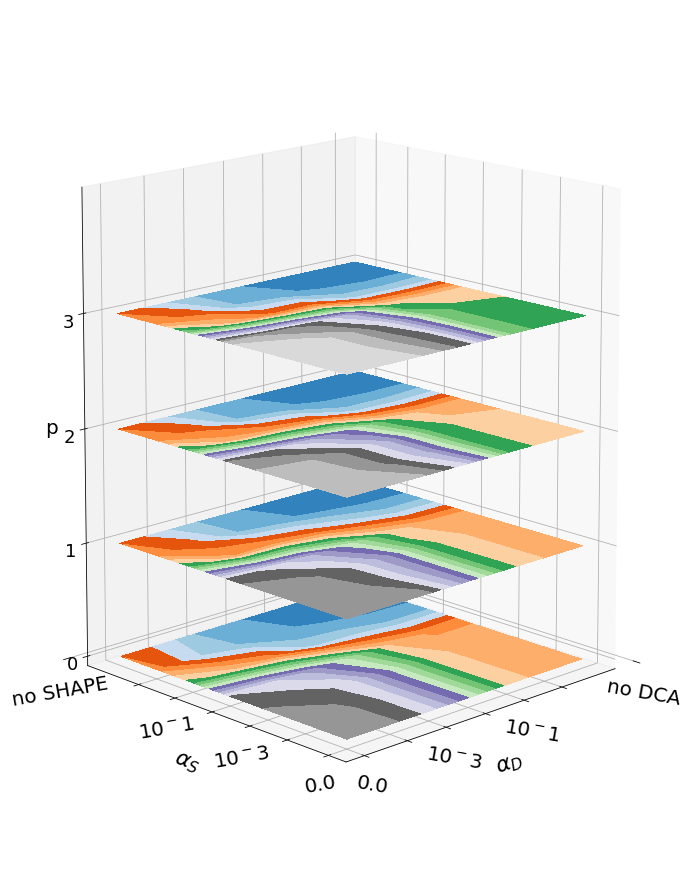
(a)

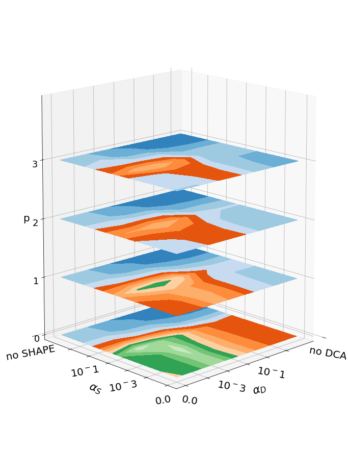
(b)

Figure 2: Population of native structure as function of hyperparameters. Population is indicated in the color scale. The optimized population of native structures, when averaged on the training set (a), is by construction a monotonically increasing function of the integer $p$ controlling the window size of the convolutional network in the reactivity channel, and a monotonically decreasing function of the regularization coefficients $\alpha_{S}$ and $\alpha_{D}$. When averaged on the leave-one-out iterations of the cross-validation (CV) procedure (b), the dependency of the optimized population of native structures on these hyperparameters becomes non-trivial, as it results from a combination of model complexity (controlled by $p$) and regularization (controlled by $\alpha_{S}$ and $\alpha_{D}$ independently). The CV procedure serves as criterion for model selection, resulting in the selection of hyperparameters $\{p=0,\alpha_{S}=0.001,\alpha_{D}=0.001\}$.

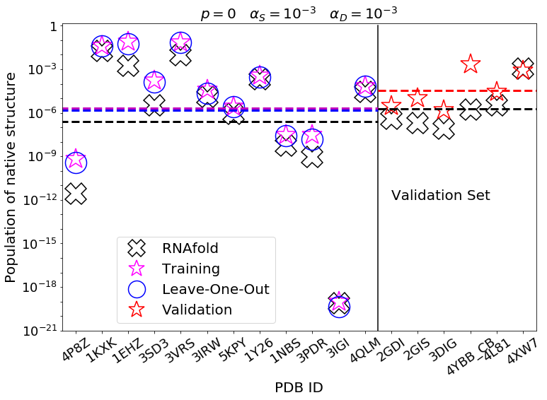
(a)

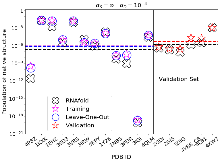
(b)

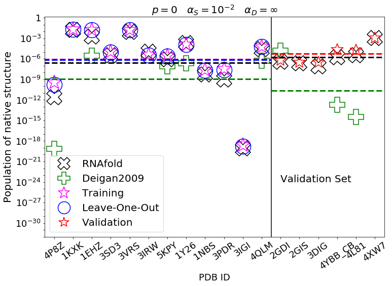
(c)

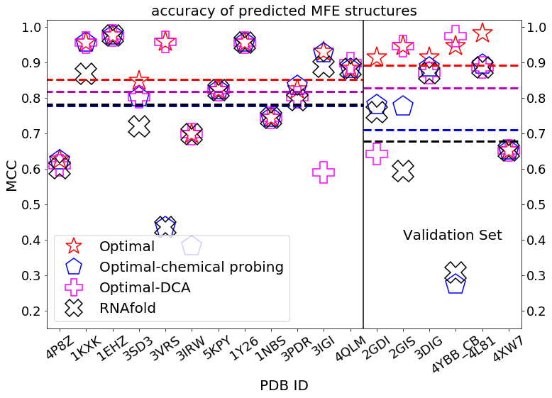
(d)

Figure 3: Comparison of results obtained with unmodified RNAfold and with selected models, respectively: populations of native structures with (a) the best performing model; (b) the best performing model with DCA data only; (c) the best performing model with chemical probing data only. (d) Matthews correlation coefficients between predicted MFE structures and reference native structures, as obtained with selected (best, DCA-only, chemical probing-only) models and with unmodified RNAfold. Hyperparameters are noted in the figure. Native structure populations obtained with unmodified RNAfold (black cross), with our trained model (magenta star on the training set, red star on the validation set) and in the leave-one-out procedure (blue circle, for each molecule the model is trained on all the other molecules in the training set) are reported. Populations obtained by mapping SHAPE reactivities into penalties with the method in Ref. [15] are reported for comparison (green plus), only for molecules studied in previous work and in panel (c) where chemical probing data only are used. The populations of native structures that we obtain with the trained model are almost always increased for molecules both in the training (left side of the vertical line) and in the validation set (right side), with overfitting occurring in a few cases, where populations lower than obtained with unmodified RNAfold are yielded.

We randomly choose a training set of 12 systems, leaving 6 others out for later validation. Since crystal structures, chemical probing data, and DCA data for different systems might be of different quality, the specific choice of the splitting might affect the overall training and validation results. We thus generate four independent random splittings, reported in Table 1. In the following we refer to splitting S3, that leads to the worst performance in the cross-validation test and to the best performance in the external validation. Results for all the splittings are reported in Supporting Information. Importantly, the external validation test is passed for all the splittings, indicating that our procedure is capable to detect overfitting with all of the tested datasets. The model complexity is controlled by means of three handles: a regularization parameter acting on the one-dimensional penalties derived from reactivities ($0\leq\alpha_{S}\leq\infty$), a regularization parameter acting on the two-dimensional penalties derived from DCA ($0\leq\alpha_{D}\leq\infty$) and an integer controlling the size of the window used for the convolutional network ($p<=3$). When the performance of the model is evaluated on the training set, the model that better fits the data is the most complex one, with no regularization term ($\alpha_{S}=\alpha_{D}=0$) and the largest tested window ($p=3$) (Fig. 2a). The geometric average of the populations of native structures increases by $\approx 11$ times with respect to that of the thermodynamic model alone. Training the model using only chemical probing data ($\alpha_{D}=\infty$), or only DCA data ($\alpha_{S}=\infty$), results in an increase of native population by $\approx$ 5 times and $\approx$ 3 times respectively, within the randomized set S3 (Table 1).

3.2 Model selection

In order to make the parametrization transferable, we perform a leave-one-out cross-validation (CV) procedure (see Materials and Methods) where one of the 12 systems at a time is left out of the training procedure and the increase in the native population for the left-out system is used to estimate transferability. Overall, the average performance of the model on the left-out system shows a non-trivial dependence on the hyperparameters (Fig. 2b). All the models yield a performance in the cross-validation test equal or better than the thermodynamic model alone, but the best performance is obtained when choosing $\alpha_{S}=0.001$, $\alpha_{D}=0.001$ and $p=0$. We select this model as the one that yields the best balance between performance and transferability. Results obtained by using different randomizations of the training set are reported in Supporting Information. Whereas the precise set of optimal hyperparameters depends on the specific training set, sets of hyperparameters that perform well on a specific set tend to perform well for all of the tested training sets.

3.3 Validation on an independent dataset

Finally, we evaluate the performance of the selected model on a dataset of 6 systems that were not seen during training. This additional test is done in the spirit of nested cross-validation [40] in order to properly evaluate the transferability of the procedure.

For the 6 test systems (splitting S3 of Table 1), the introduced procedure leads to a boost of the population of the native structure by $\approx$ 19 times, on average (Fig. 3a, right side of the vertical line), when using the selected model $\{\alpha_{S}=0.001,\alpha_{D}=0.001,p=0\}$. A side effect of targeting the population of native structures for model optimization and selection is the increase in the similarity between the predicted minimum free energy (MFE) and the experimental structures. This similarity can be quantified using the Matthews Correlation Coefficient (MCC) [41], that is routinely used to benchmark RNA structure prediction [42]. Its average on the validation set is increased from $0.68$ to $0.89$ (Fig. 3d, right side). Specific changes in the predicted secondary structures are reported in detail in Fig. 4, where reference secondary structures are compared with MFE predictions made with unmodified RNAfold and with the selected model. In particular, for 2GDI (Fig. 4a-c) our model recovers the correct structure of the 3-way junction loop (4-5:41-47:72-75); for 2GIS (Fig. 4d-f) it recovers the correct structures of the hairpin loop (23-29) and the internal loop (17-21:31-38); for 3DIG (Fig. 4g-i) the correct bulge loop (84-85:109-111) is recovered; for 4YBB (Fig. 4j-l) the bulge loops (30-31:51-54) and (17-18:65-67), the internal loops (23-28:56-60) and (71-79:97-105), the 3-way junction (10-16:68-70:106-110) and the hairpin loop (86-90); for 4L81 (Fig. 4m-o) the 4-way junction (5-10:21-22:51-53:66-67) is correctly predicted; for 4XW7 (Fig. 4p-r) we have no change in MFE prediction with respect to unmodified RNAfold. Considering all of the tested splittings of the dataset, the average MCC of minimum free energy structure predictions is increased from $0.72\pm 0.22$ to $0.90\pm 0.10$, implying both an increased average and a decreased variance (details in Supporting Information).

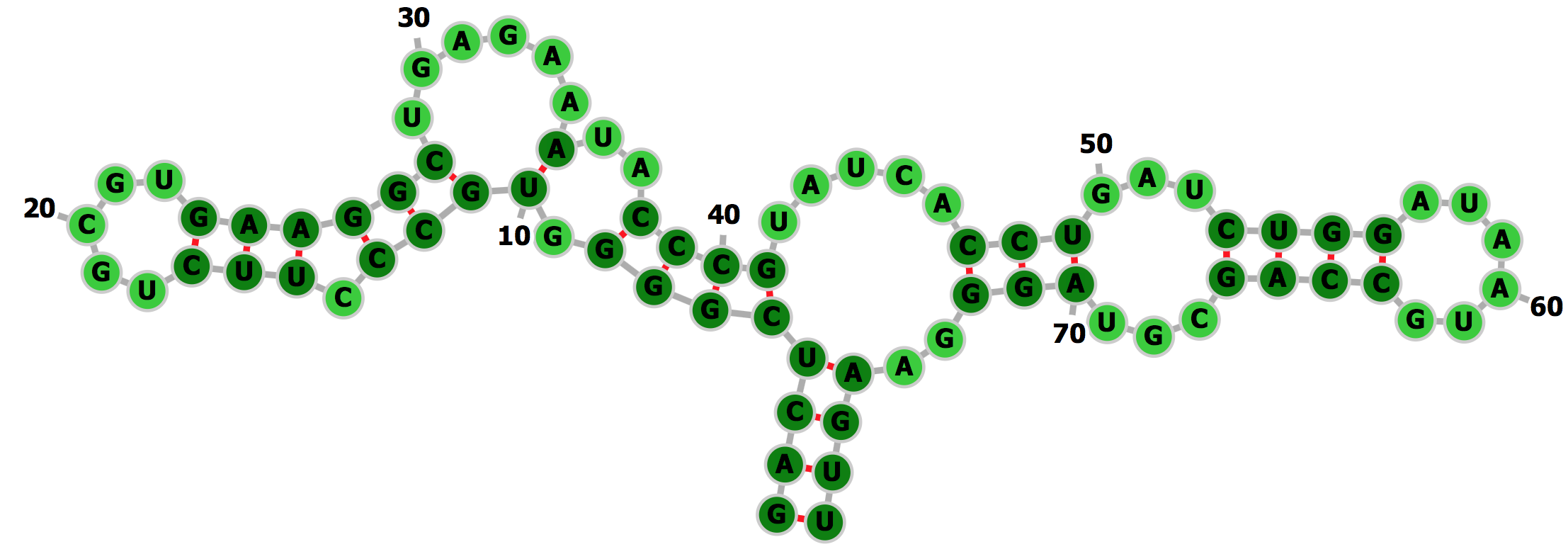
(a) Reference

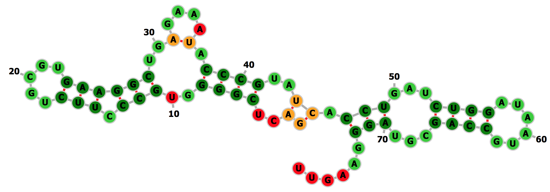
(b) RNAfold (0.76)

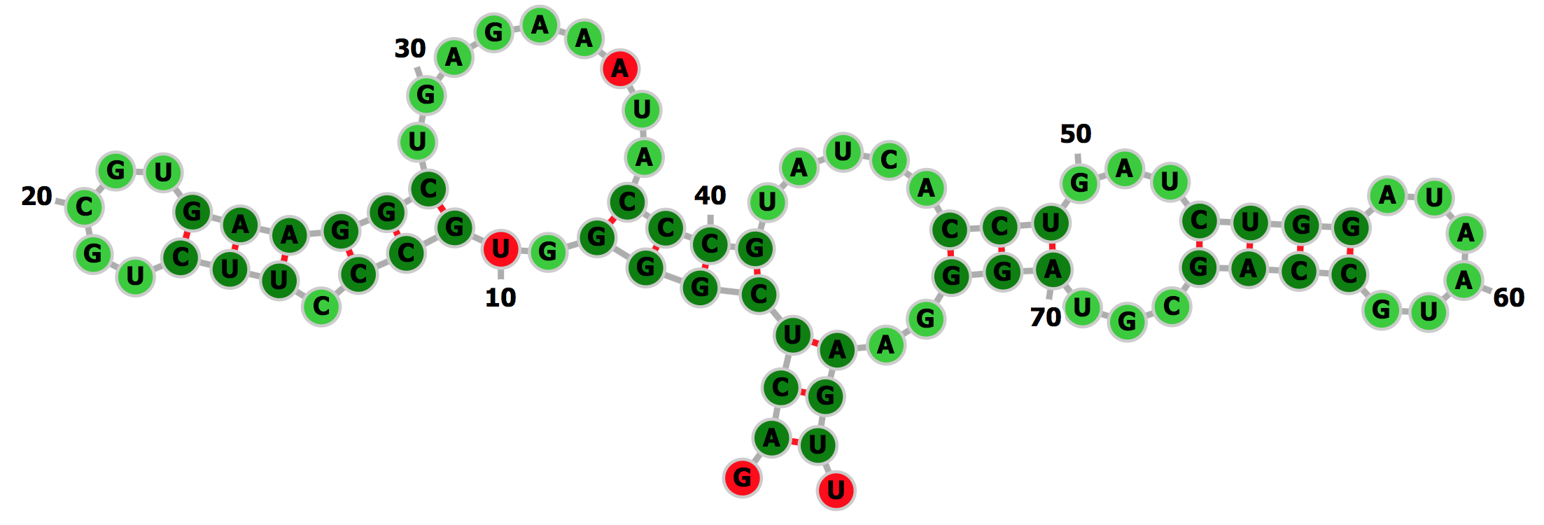
(c) Trained model (0.91)

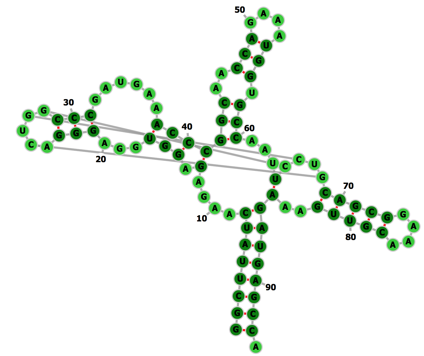
(d) Reference

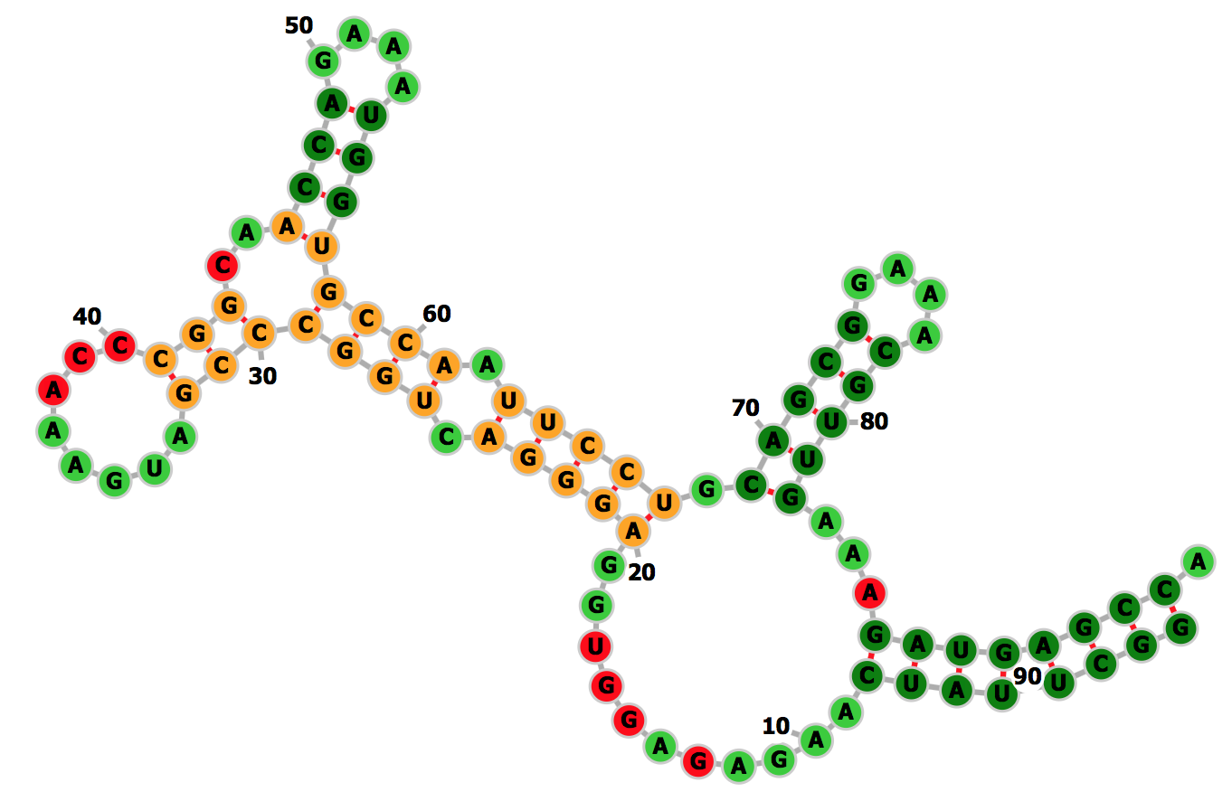
(e) RNAfold (0.59)

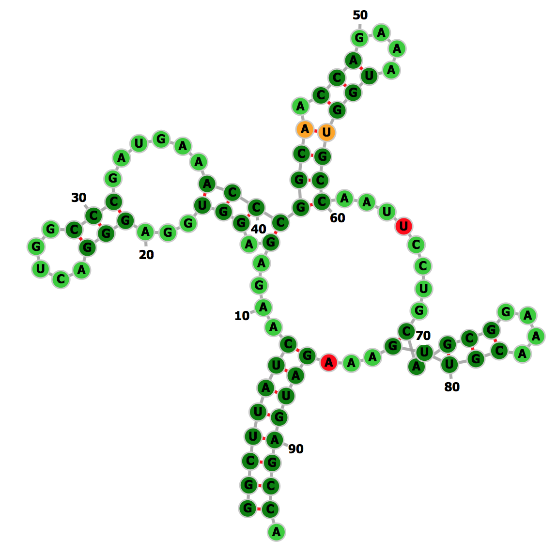
(f) Trained model (0.95)

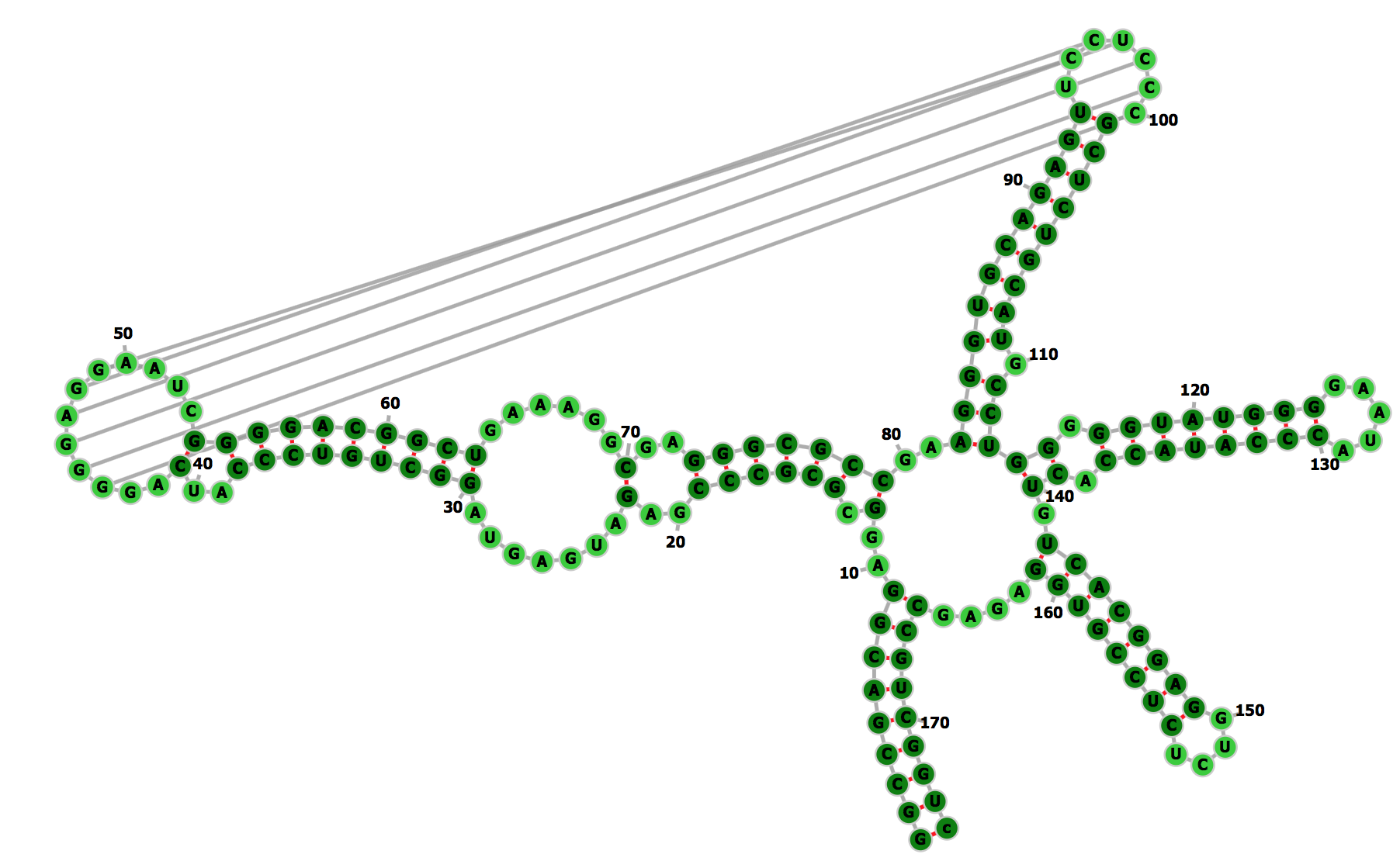
(g) Reference

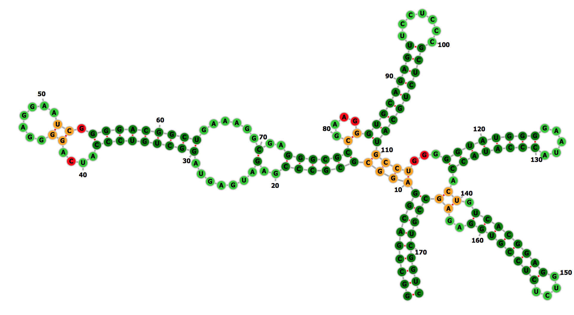
(h) RNAfold (0.87)

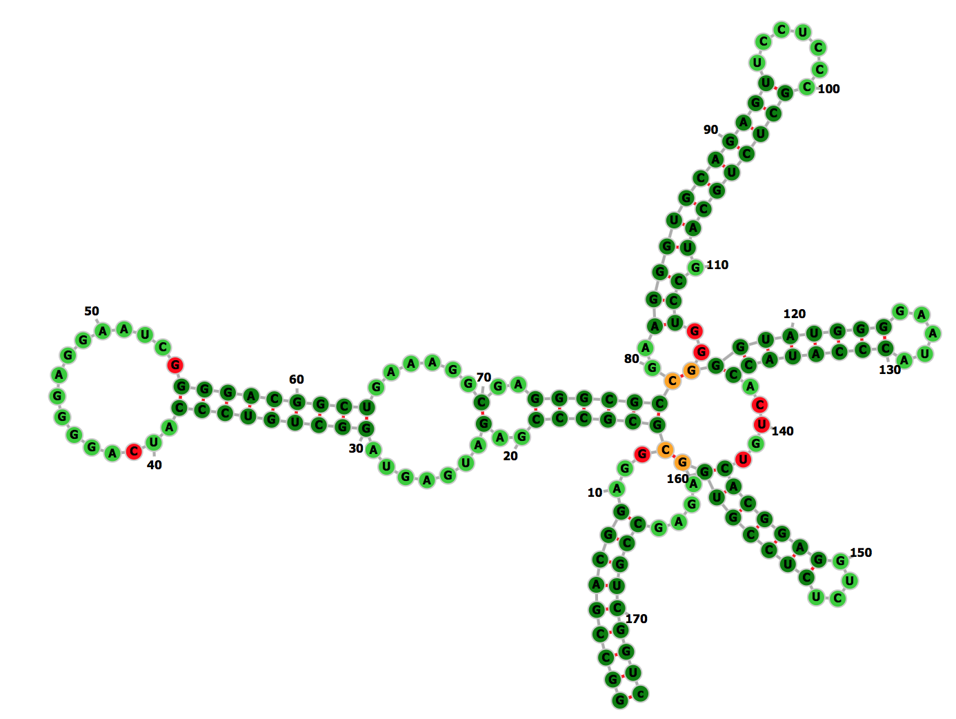
(i) Trained model (0.91)

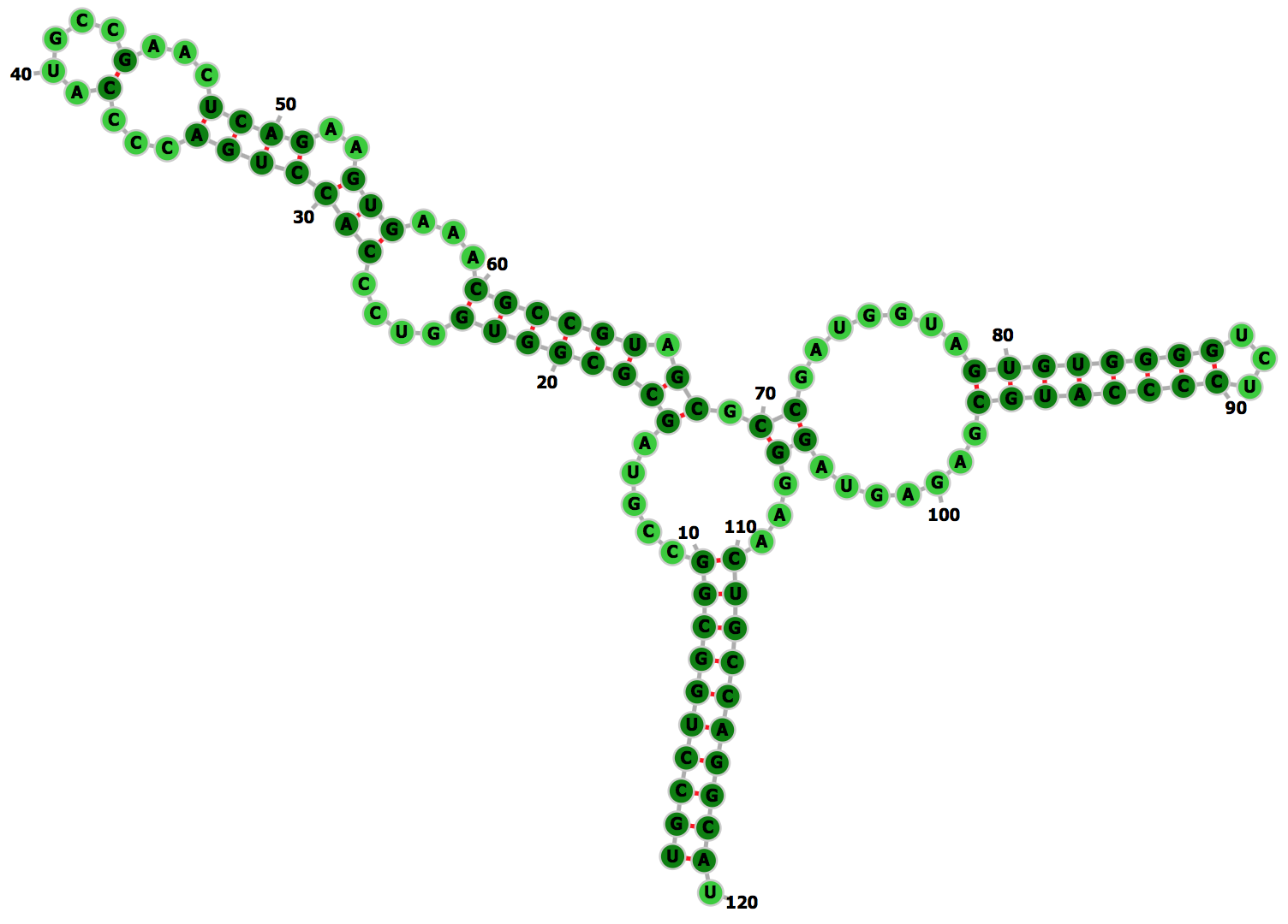
(j) Reference

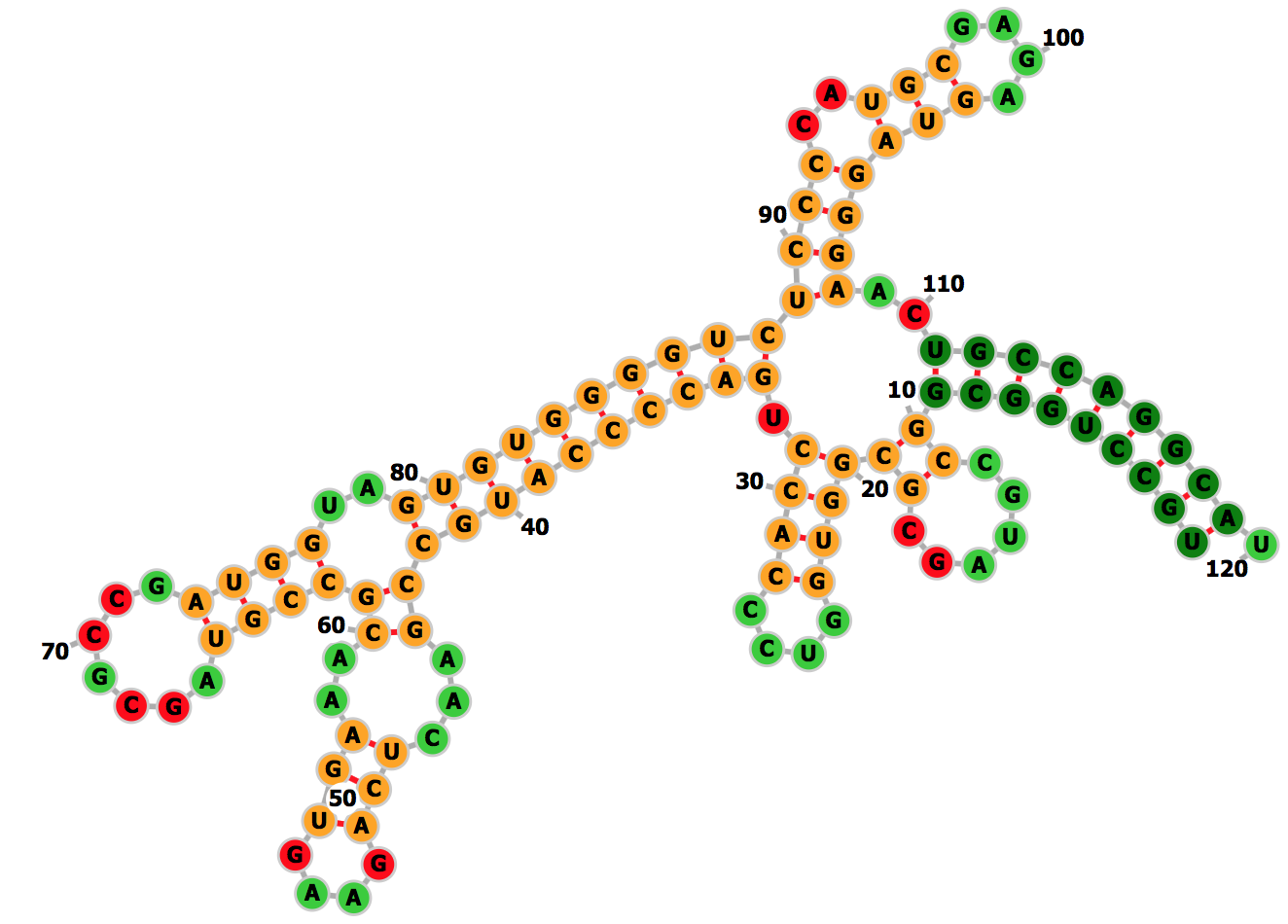
(k) RNAfold (0.31)

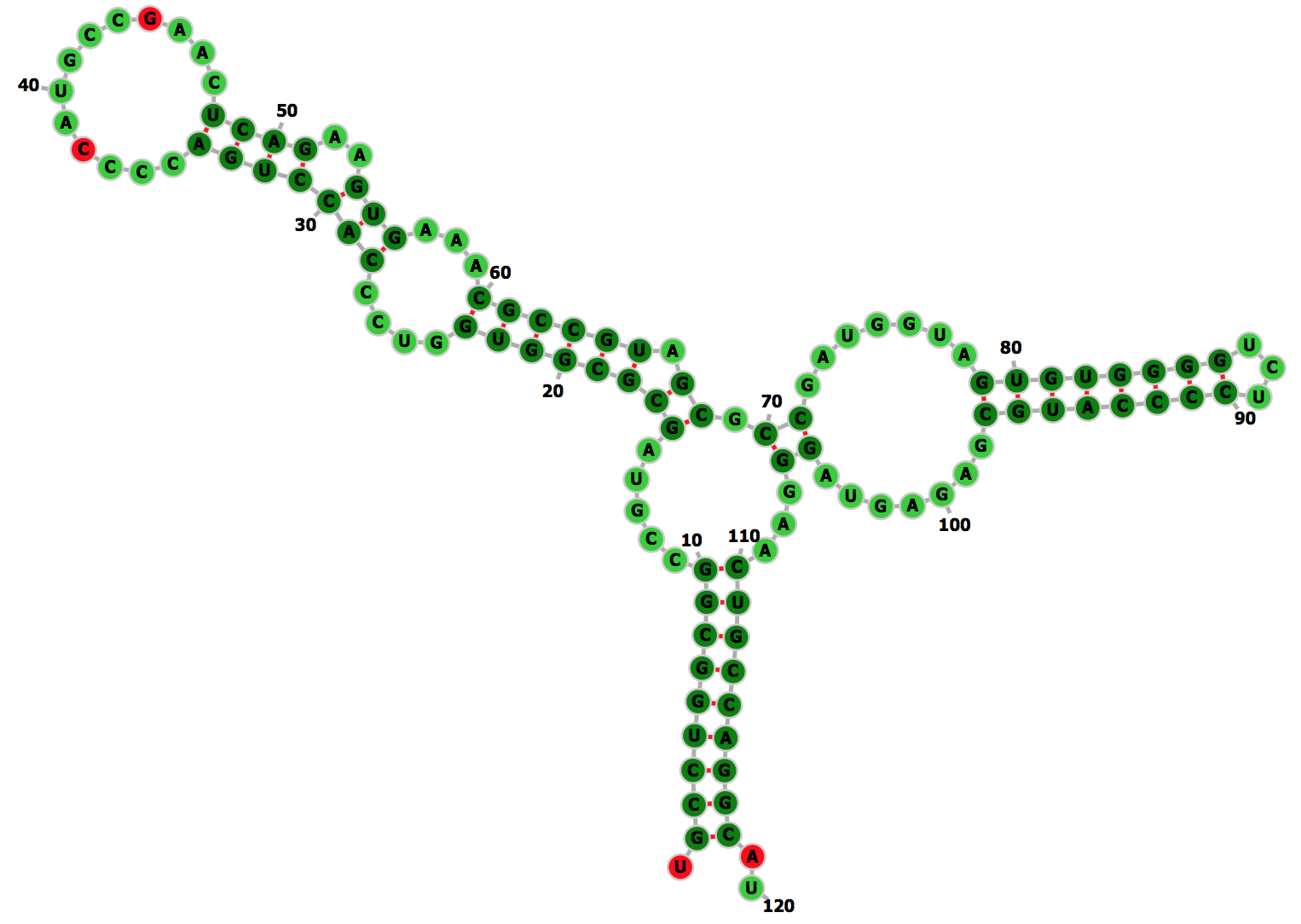
(l) Trained model (0.95)

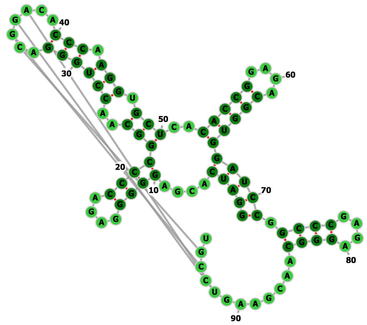
(m) Reference

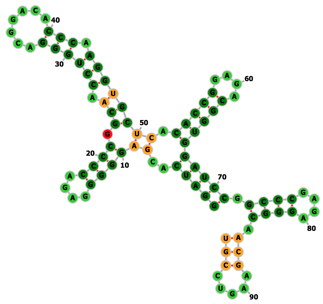
(n) RNAfold (0.87)

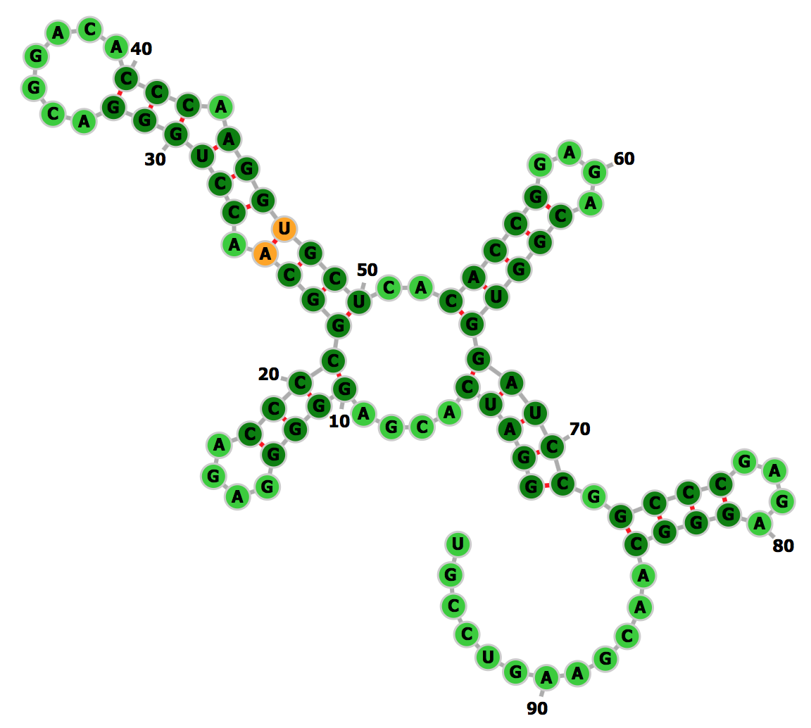
(o) Trained model (0.98)

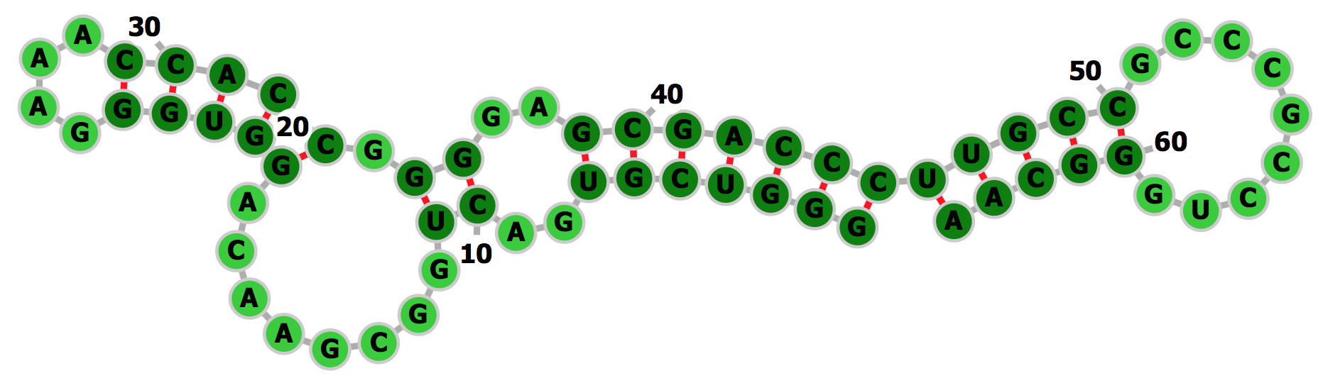
(p) Reference

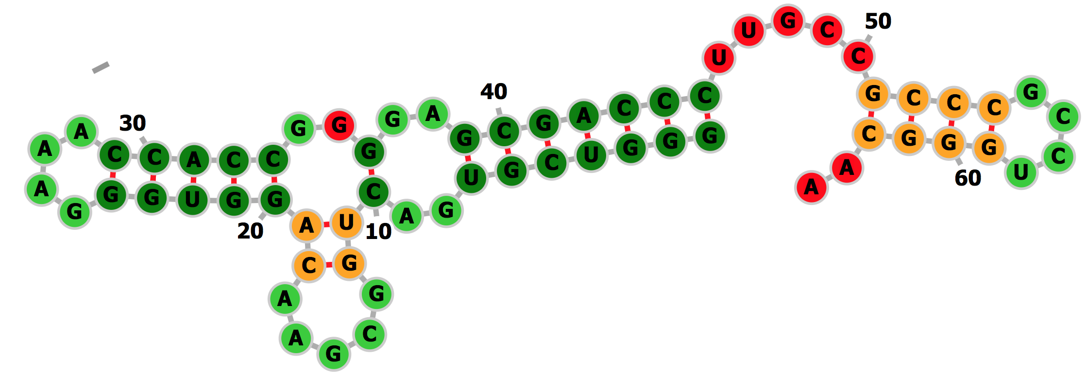
(q) RNAfold (0.65)

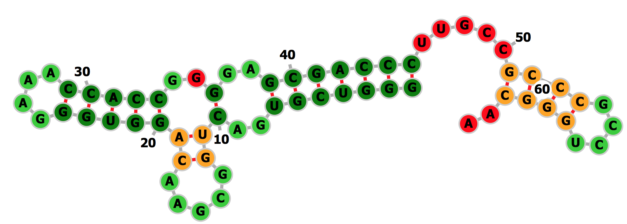
(r) Trained model (0.65)

Figure 4: Minimum free energy (MFE) structure predictions. For each system in the validation set, reference native structure is compared with predicted MFEs. Correctly predicted base pairs (true positives) and unpaired nucleotides (true negatives) are reported in dark green and lime green, respectively. Wrongly predicted base pairs (false positives) and unpaired nucleotides (false negatives) are reported in orange and red, respectively. MCC between prediction and reference is reported in parenthesis. All the relevant improvements in the prediction of these structures are reported in detail in section Results. All secondary structure diagrams are drawn with forna [43].

As can be seen from Fig. 4, some of the structures in the dataset contain pseudoknots. This kind of pairing is forbidden in RNAfold structure predictions, thus we do not include it in the estimation of MCC. Nontheless, data from both chemical probing and coevolution analysis in principle contain information about pseudoknots, and it is possible to examine how reactivities and DCA scores of pseudoknotted nucleotides are mapped into pairing penalties in our optimal model. We notice that the average value of pairwise DCA penalties applied to pseudoknot pairs $\langle\lambda_{ij}\rangle_{PK}=-0.087$ is comparable to the average of those applied to base pairs $\langle\lambda_{ij}\rangle_{BP}=-0.094$, so that they have almost the same effect in favouring pairing (free-energy term $\lambda_{ij}s_{ij}<0$ for $s_{ij}=1$). The difference between the two values is negligible when compared with the average DCA penalty applied to unpaired nucleotides $\langle\lambda_{ij}\rangle_{UP}=0.447$. Reactivity-driven single-point penalties favour unpaired states on average (free-energy term $-\lambda_{i}s_{i}>0$ for $s_{i}=1$), but the effect on pseudoknotted nucleotides $\langle\lambda_{i}\rangle_{PK}=-0.142$ and on base-paired nucleotides $\langle\lambda_{i}\rangle_{BP}=-0.125$ is approximatley half of that on unpaired nucleotides $\langle\lambda_{i}\rangle_{UP}=-0.284$. Even though in our optimal model the pairing of pseudoknotted nucleotides is boosted with almost the same intensity of base-paired nucleotides, eventually small values are predicted for the corresponding pairing probabilites (see Supporting Information). This is due to the fact that the thermodynamic model only allows structures with nested pairs.

It is also possible to test the scenarios where only DCA data or only chemical probing data are available. In scenarios where only DCA information is used ($\alpha_{S}=\infty$), the best performance in CV is obtained using the model with $\alpha_{D}=0.0001$ ($10\times$ increase in population, average MCC $=0.83$, Fig. 3b and d). This model is thus transferable to the validation set yielding a significant increase in both the population of the native structures and in MFE structure accuracy. In the case of chemical probing-only information ($\alpha_{D}=\infty$), the best performance in CV is obtained using the model with hyperparameters $\alpha_{S}=0.01$ and $p=0$ ($3\times$ increase in population, average MCC $=0.71$, Fig. 3c and d). Interestingly, whereas reactivity-only models perform systematically better in training than DCA-only models, their performance in CV is systematically lower, suggesting a lower transferability to unseen data, and thus a larger risk for reactivity-driven penalties to be overfitted. This might be related to the high heterogeneity of the chemical probing data used here, that makes it difficult to fit transferable parameters.

Our procedure to compute pairing penalties from SHAPE reactivities can be compared with the one introduced by Deigan et. al. [15]. Since the Deigan’s method requires SHAPE data normalized with a different procedure, we use normalized reactivities reported in Ref. [29]. Remarkably, our procedure leads to significantly better results both for molecules that are included in the training set (e.g., 4P8Z, 1EHZ, 5KPY,1Y26,4QLM in Fig. 3c), and for most of the RNAs included in the validation set (4YBB_CB and 4L81 in the right side of Fig. 3c).

3.4 Interpretation of parameters

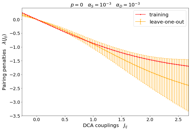
(a)

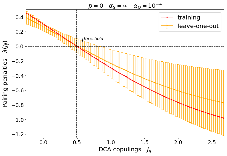
(b)

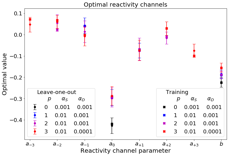
(c)

Figure 5: Properties of the optimized neural network. For the DCA channel, the optimized function mapping DCA couplings $J_{ij}$ into pairing penalties $\lambda_{ij}$, for both (a) the selected model and (b) the best performing model with restriction to only DCA input. When trained on the whole training set (red) the activation function is consistent with the average on the leave-one-out training subsets (orange). Error bars are computed as standard deviations and are significantly lower in the region of DCA couplings around zero, as couplings lying in that region are more frequent. The trained function maps high (respectively, low) DCA coupling values to penalties favoring (respectively, disfavoring) the corresponding pairings, thus affecting the population of the structures including the specific pair. When restricting to (b) models including only DCA input, the threshold value of the coupling $J^{threshold}$ between disfavored and favored pairing corresponds to the zero of the activation function, as indicated by the dashed line. For the chemical mapping channel, (c) optimal values of model parameters are shown for the selected model (black) with hyperparameters $\{\alpha_{S}=0.001,\alpha_{D}=0.001,p=0\}$, and for the sub-optimal models with $p>0$. All the training results (cross) lie within the leave-one-out errors (dots with error bars), indicating robustness of the minimization procedure against cross-validation. Coefficients $\{a_{-k},\dots,a_{+k}\},\quad k>0$ weighting reactivities up to the $k$-th nearest-neighbors of a nucleotide, report the minor contributions of the local reactivity pattern in addition to the nucleotide’s own reactivity.

In principle, different randomizations of the training set yield different hyperparameters and parameters for the functions implemented in the selected model. Here we continue focusing on splitting S3. The selected model is defined by hyperparameters $\{\alpha_{S}=0.001,\alpha_{D}=0.001,p=0\}$. Results for different splittings are similar and are reported in Supporting Information.

DCA channel. DCA couplings are mapped into pairing penalties through a double-layered neural network, resulting in a non-linear function reported in Fig. 5a. Pairing penalties are found to decrease with increasing DCA coupling value, consistent with the interpretation that large couplings should correspond to co-evolutionarily related and thus likely paired nucleobases [18]. A more detailed interpretation of these pairing penalties is possible if we restrict to models taking only DCA couplings as input ($\alpha_{S}=\infty$). The corresponding non-linear function is reported in Fig. 5b. The overall shape is consistent with that obtained fitting all the data (Fig. 5a), but the zero of this function can be straightforwardly interpreted as the threshold for penalizing or favoring base pairing. The resulting value is $J^{\textrm{threshold}}=0.49$ consistent with the typical thresholds obtained in [32] with a different optimization criterion, based on the accuracy of contact predictions, and fitted on a larger dataset, thus confirming the transferability of the non-linear function reported here.

Reactivity channel. Chemical probing reactivities are mapped into penalties affecting the population of individual nucleotide pairing states through a single convolutional layer with a linear activation function. When evaluated on the training set, the best performance is obtained with models including up to the maximum tested number of nearest neighbors ($p=3$). In these models, for each nucleotide, the network input vector includes reactivities from the third nearest-neighbor upstream to its third nearest-neighbor downstream along the sequence. The activation coefficients $\{a_{k},\quad k=-3,\dots,+3\}$ weight the contribution of each nucleotide in the neighbor window. Despite the performance improvement on the training set, transferability to data not seen during the training phase is best preserved in the model that retains only the contribution from the $a_{0}$ term, confirming that the reactivity of a nucleotide is maximally affected by its pairing state. We notice that SHAPE reactivity has been correlated with sugar flexibility [44, 45, 46], and is only indirectly related to the pairing state of a nucleotide. Nevertheless, reactivity information can be used to systematically improve predictions at the base-pairing level. In particular, $a_{0}<0$ (see Fig. 5c, black) so that the pairing of a highly reactive nucleotide is unfavoured and vice-versa for nucleotides with low reactivity. On the other hand, the best (suboptimal) neighbor-including models (i.e., with $p>0$) still yield comparable results with respect to the selected one and significant improvements as well with respect to thermodynamic model alone. Figure 5c reports the sets of optimal parameters with $p>0$. We notice that at each increment of $p$, when two new parameters $a_{p}$ and $a_{-p}$ are introduced, all the shared subsets $\{a_{p-1},\dots,a_{-p+1}\}$ overlap significantly, and a number of features are shared as well. First, for all the optimal choices of $p>0$, the sum of the weights $\sum_{i=-p}^{p}a_{i}$ is negative, so that the pairing of a nucleotide in a highly reactive region is unfavored, and vice-versa for regions of low reactivity. The largest contribution still arises from the $a_{0}$ term, but it is slightly lower in absolute value, to compensate for neighbor corrections. For each pair (downstream and upstream) of $k$-th nearest-neighbours, the combination of the $a_{0}$ and $a_{+k}$ ($a_{-k}$) contributions can be interpreted as a forward (backward) finite-difference operator estimating the $k$-th order derivative of the reactivity with respect to the position in the sequence. These contributions map local downward trends of the reactivity profile into pairing penalties, thus providing a sort of normalization for the reactivity of the central nucleotide with respect to that of its neighbors. As the order of the derivatives increase from the first, weights become lower such that the corresponding corrections progressively decrease in importance. It is interesting to notice that the finer these corrections are, the more the corresponding parameters tend to be overfitted to the training set.

4 DISCUSSION

In this work we build a network that can be used to predict RNA structure taking as an input RNA sequence, chemical probing reactivities, and DCA scores. Whereas reactivities and DCA scores are processed through standard linear or non-linear units, RNA sequence enters through a thermodynamic model. A crucial ingredient that we introduce here are the derivatives of the result of the thermodynamic model with respect to the pairing penalties, that allow the network to be trained using gradient-based machine learning techniques.

We built up a total of 196 models to map simultaneously reactivities and DCA scores into free-energy terms coupling, respectively, the pairing state of individual nucleotides and that of specific pairs of nucleotides. Each model is defined by tunable hyperparameters controlling the width of the windows used to process reactivities and the strength of the regularization terms applied to chemical probing and DCA data. The dataset is a priori split randomly into a training set and a validation set (12 and 6 systems respectively). Training, model selection and validation are repeated for different random splittings of the dataset, in order to decrease the chance of introducing a bias towards specific structures or features, and ensuring the robustness of the procedure. The whole procedure, from training to model selection, is automatic so that new parameters could be straightforwardly obtained using new chemical probing and DCA data and new crystallographic structures, allowing for a continuous refinement of the proposed structure prediction protocol. Training one model required 20 minimizations that were performed in parallel on nodes containing 2 E5-2683 CPU each, using 20 cores. Each minimization took approximately 30 minutes, though the exact time depends on the value of $p$ and on the system size. 4x7x7=196 minimizations were done to scan the hyperparameter space. 12 separate models needed to be trained for the leave-one-out. Notably, the dependence between the minimizations (see Materials and Methods) can be taken into account (see scripts in Supporting Information) allowing them to be largely run in parallel. In practice, if 288 nodes are simultaneously available, the full minimization for 12 systems can be run in approximately 8 hours. In the dataset we used, some reactivities are taken from available experimental data. Other reactivities are measured here for the first time so as to increase the number of systems for which both co-evolutionary data and reactivities are available. DCA scores are based on ClustalW alignments [33] so that they are not manually curated with prior structural information. We notice however that classification of sequences in RFAM is performed including structural information, when available. In addition, co-evolutionary information might be difficult to extract for poorly conserved long non-coding RNAs. All the reactivity profiles and DCA score matrices are reported in Supporting Information Section S2. All the results obtained with different randomization of the validation set are reported in Supporting Information so that different sets of parameters can be easily tested.

The model selected via CV is defined by hyperparameters $\{p=0,\alpha_{S}=0.001,\alpha_{D}=0.001\}$. The best performance/transferability trade-off is thus obtained when not incorporating reactivities from neighboring nucleotides in the pairing state of a nucleotide. This model is systematically capable of predicting a higher population for the native structure. The model that is selected using only chemical probing data yields better results in population than what obtained with Deigan’s method [15], which is accounted for best state-of-the-art method [47] among those based on SHAPE reactivities only. Results obtained with our selected model confirm that the reactivity of a nucleotide is a good indicator of its own pairing state [47]. We also observe that the reactivity of neighbors correlate too with the pairing state of a nucleotide (see Supporting Information). However, the pairing state of neighboring nucleotides is implicitly taken into account in the RNAfold model, that includes energetic contributions for consecutive base pairs, implying that the explicit inclusion might not be required. More precisely, the need for a larger number of parameters to be trained when increasing the $p$ hyperparameter might not be compensated by a sufficient improvement in the prediction performance. Interestingly, in a previous version of this work based on a smaller dataset and on different thermodynamic parameters [7] the most transferable model identified had $p=2$ (see https://arxiv.org/abs/2004.00351v1). In perspective, the model can be extended to include additional features of the chemical probing experiments that may be related to non-canonical interactions and three-dimensional structure.

Although our selected model is trained to maximize the population of the individual reference structure as obtained by crystallization experiments, it can still report alternative structures. Whereas we did not investigate this issue here, alternative low-population states might be highly relevant for function. Compatibly with that, the absolute population of the native structure remains significantly low (from $\approx 10^{-8}$ to $\approx 10^{-7}$), but is still one of the highest in the ensemble. In particular, the individual structure with highest population (minimum free-energy structure) with our method is closer to the reference crystallographic structure than the one predicted by thermodynamic parameters alone on systems not seen during training.

Importantly, all the data and the used scripts are available and can be used to fit the model over larger datasets. In order to avoid overfitting, we suggest to repeat the leave-one-out procedure to select the most transferable model, whenever new independent data is added to the dataset. Scripts for training and model selection are reported in Supporting Information. In principle the model can be straighforwardly extended to include any chemical probing data that putatively correlates with base pairing state [13] or other types of experimental information that correlate with base-pairing probabilities [50]. Training on a larger set of reference structures and using more types of experimental data will make the model more robust and open the way to the reliable structure determination of non-coding RNAs.

References

- [1] Cech, T. R. (2000) The ribosome is a ribozyme. Science, 289(5481), 878–879.
- [2] Doudna, J. and Cech, T. (2002) The chemical repertoire of natural ribozymes. Nature, 418(6894), 222–228.
- [3] Morris, K. V. and Mattick, J. S. (2014) The rise of regulatory RNA. Nat. Rev. Genet., 15(6), 423.
- [4] Wan, Y., Kertesz, M., Spitale, R. C., Segal, E., and Chang, H. Y. (2011) Understanding the transcriptome through RNA structure. Nat. Rev. Genet., 12(9), 641.
- [5] Cooper, T. A., Wan, L., and Dreyfuss, G. (2009) RNA and disease. Cell, 136(4), 777–793.
- [6] Tinoco, I., Borer, P. N., Dengler, B., Levine, M. D., Uhlenbeck, O. C., Crothers, D. M., and Gralla, J. (1973) Improved estimation of secondary structure in ribonucleic acids. Nature, 246(150), 40–41.
- [7] Xia, T., SantaLucia Jr, J., Burkard, M. E., Kierzek, R., Schroeder, S. J., Jiao, X., Cox, C., and Turner, D. H. (1998) Thermodynamic parameters for an expanded nearest-neighbor model for formation of RNA duplexes with Watson- Crick base pairs. Biochemistry, 37(42), 14719–14735.
- [8] Nussinov, R., Pieczenik, G., Griggs, J. R., and Kleitman, D. J. (1978) Algorithms for loop matchings. SIAM J. Appl. Math., 35(1), 68–82.
- [9] Lorenz, R., Bernhart, S. H., Zu Siederdissen, C. H., Tafer, H., Flamm, C., Stadler, P. F., and Hofacker, I. L. (2011) ViennaRNA Package 2.0. Algorithms Mol. Biol., 6(1), 26.
- [10] Wuchty, S., Fontana, W., Hofacker, I. L., and Schuster, P. (1999) Complete suboptimal folding of RNA and the stability of secondary structures. Biopolymers, 49(2), 145–165.
- [11] Dethoff, E. A., Petzold, K., Chugh, J., Casiano-Negroni, A., and Al-Hashimi, H. M. (2012) Visualizing transient low-populated structures of RNA. Nature, 491(7426), 724–728.
- [12] Serganov, A. and Nudler, E. (2013) A decade of riboswitches. Cell, 152(1), 17–24.
- [13] Weeks, K. M. (2010) Advances in RNA structure analysis by chemical probing. Curr. Opin. Struct. Biol., 20(3), 295–304.
- [14] Merino, E. J., Wilkinson, K. A., Coughlan, J. L., and Weeks, K. M. (2005) RNA structure analysis at single nucleotide resolution by selective 2′-hydroxyl acylation and primer extension (SHAPE). J. Am. Chem. Soc., 127(12), 4223–4231.
- [15] Deigan, K. E., Li, T. W., Mathews, D. H., and Weeks, K. M. (2009) Accurate SHAPE-directed RNA structure determination. Proc. Natl. Acad. Sci. U.S.A., 106(1), 97–102.
- [16] Spitale, R. C., Flynn, R. A., Zhang, Q. C., Crisalli, P., Lee, B., Jung, J.-W., Kuchelmeister, H. Y., Batista, P. J., Torre, E. A., Kool, E. T., et al. (2015) Structural imprints in vivo decode RNA regulatory mechanisms. Nature, 519(7544), 486.
- [17] Morcos, F., Pagnani, A., Lunt, B., Bertolino, A., Marks, D. S., Sander, C., Zecchina, R., Onuchic, J. N., Hwa, T., and Weigt, M. (2011) Direct-coupling analysis of residue coevolution captures native contacts across many protein families. Proc. Natl. Acad. Sci. U.S.A., 108(49), E1293–E1301.
- [18] De Leonardis, E., Lutz, B., Ratz, S., Cocco, S., Monasson, R., Schug, A., and Weigt, M. (2015) Direct-coupling analysis of nucleotide coevolution facilitates RNA secondary and tertiary structure prediction. Nucleic Acids Res., 43(21), 10444–10455.
- [19] Weinreb, C., Riesselman, A. J., Ingraham, J. B., Gross, T., Sander, C., and Marks, D. S. (2016) 3D RNA and functional interactions from evolutionary couplings. Cell, 165(4), 963–975.
- [20] Lavender, C. A., Lorenz, R., Zhang, G., Tamayo, R., Hofacker, I. L., and Weeks, K. M. (2015) Model-Free RNA Sequence and Structure Alignment Informed by SHAPE Probing Reveals a Conserved Alternate Secondary Structure for 16S rRNA. PLoS Comput. Biol., 11(5), 1–19.
- [21] Lu, X.-J., Bussemaker, H. J., and Olson, W. K. (07, 2015) DSSR: an integrated software tool for dissecting the spatial structure of RNA. Nucleic Acids Res., 43(21), e142–e142.
- [22] Andronescu, M., Condon, A., Hoos, H. H., Mathews, D. H., and Murphy, K. P. (07, 2007) Efficient parameter estimation for RNA secondary structure prediction. Bioinformatics, 23(13), i19–i28.
- [23] McCaskill, J. S. (1990) The equilibrium partition function and base pair binding probabilities for RNA secondary structure. Biopolymers, 29(6-7), 1105–1119.
- [24] Wilkinson, K. A., Merino, E. J., and Weeks, K. M. (2006) Selective 2’-hydroxyl acylation analyzed by primer extension (SHAPE): quantitative RNA structure analysis at single nucleotide resolution. Nat. Protoc., 1(3), 1610–6.
- [25] Mörl, M. and Schmelzer, C. (1993) A simple method for isolation of intact RNA dried from polyacrylamide gels. Nucleic Acids Res., 21(8), 2016–2016.
- [26] Karabiber, F., McGinnis, J. L., Favorov, O. V., and Weeks, K. M. (2013) QuShape: Rapid, accurate, and best-practices quantification of nucleic acid probing information, resolved by capillary electrophoresis. RNA, 19(1), 63–73.
- [27] Aviran, S., Lucks, B., and Patcher, L. (2011) RNA structure characterization from chemical mapping experiments. 49th Annual Allerton Conference on Communication, Control, and Computing (Allerton), pp. 1743–1750.
- [28] Cordero, P., Lucks, J. B., and Das, R. (2012) An RNA Mapping DataBase for curating RNA structure mapping experiments. Bioinformatics, 28(22), 3006–3008.
- [29] Loughrey, D., Watters, K. E., Settle, A. H., and Lucks, J. B. (2014) SHAPE-Seq 2.0: systematic optimization and extension of high-throughput chemical probing of RNA secondary structure with next generation sequencing. Nucleic Acids Res., 42(21), e165.
- [30] Hajdin, C. E., Bellaousov, S., Huggins, W., Leonard, C. W., Mathews, D. H., and Weeks, K. M. (2013) SHAPE-directed RNA structure modeling. Proc. Natl. Acad. Sci. U.S.A., 110(14), 5498–5503.
- [31] Poulsen, L. D., Kielpinski, L. J., Salama, S. R., Krogh, A., and Vinther, J. (2015) SHAPE Selection (SHAPES) enrich for RNA structure signal in SHAPE sequencing-based probing data. RNA, 21(5), 1042–1052.
- [32] Cuturello, F., Tiana, G., and Bussi, G. (2020) Assessing the accuracy of direct-coupling analysis for RNA contact prediction. RNA, 26(5), 637–647.
- [33] Larkin, M., Blackshields, G., Brown, N., Chenna, R., McGettigan, P., McWilliam, H., Valentin, F., Wallace, I., Wilm, A., Lopez, R., Thompson, J., Gibson, T., and Higgins, D. (09, 2007) Clustal W and Clustal X version 2.0. Bioinformatics, 23(21), 2947–2948.
- [34] Zarringhalam, K., Meyer, M. M., Dotu, I., Chuang, J. H., and Clote, P. (2012) Integrating chemical footprinting data into RNA secondary structure prediction. PLoS One, 7(10), e45160.
- [35] Washietl, S., Hofacker, I. L., Stadler, P. F., and Kellis, M. (2012) RNA folding with soft constraints: reconciliation of probing data and thermodynamic secondary structure prediction. Nucleic Acids Res., 40(10), 4261–4272.
- [36] Goodfellow, I., Bengio, Y., and Courville, A. (2016) Deep learning, MIT press, .
- [37] Virtanen, P., Gommers, R., Oliphant, T. E., Haberland, M., Reddy, T., Cournapeau, D., Burovski, E., Peterson, P., Weckesser, W., Bright, J., et al. (2020) SciPy 1.0: fundamental algorithms for scientific computing in Python. Nat. Methods, 17, 261–272.
- [38] Burley, S. K., Berman, H. M., Bhikadiya, C., Bi, C., Chen, L., Di Costanzo, L., Christie, C., Dalenberg, K., Duarte, J. M., Dutta, S., et al. (2018) RCSB Protein Data Bank: biological macromolecular structures enabling research and education in fundamental biology, biomedicine, biotechnology and energy. Nucleic Acids Res., 47(D1), D464–D474.
- [39] Nawrocki, E. P., Burge, S. W., Bateman, A., Daub, J., Eberhardt, R. Y., Eddy, S. R., Floden, E. W., Gardner, P. P., Jones, T. A., Tate, J., et al. (2014) Rfam 12.0: updates to the RNA families database. Nucleic Acids Res., 43(D1), D130–D137.
- [40] Cawley, G. C. and Talbot, N. L. (2010) On over-fitting in model selection and subsequent selection bias in performance evaluation. J. Mach. Learn. Res., 11(Jul), 2079–2107.
- [41] Matthews, B. (1975) Comparison of the predicted and observed secondary structure of T4 phage lysozyme. Biochim. Biophys. Acta, 405(2), 442 – 451.
- [42] Miao, Z., Adamiak, R. W., Antczak, M., Batey, R. T., Becka, A. J., Biesiada, M., Boniecki, M. J., Bujnicki, J. M., Chen, S.-J., Cheng, C. Y., et al. (2017) RNA-Puzzles Round III: 3D RNA structure prediction of five riboswitches and one ribozyme. RNA, 23(5), 655–672.
- [43] Kerpedjiev, P., Hammer, S., and Hofacker, I. L. (2015) Forna (force-directed RNA): Simple and effective online RNA secondary structure diagrams. Bioinformatics, 31(20), 3377–3379.
- [44] Weeks, K. M. and Mauger, D. M. (2011) Exploring RNA structural codes with SHAPE chemistry. Acc. Chem. Res., 44(12), 1280–1291.
- [45] Mlýnský, V. and Bussi, G. (2018) Molecular dynamics simulations reveal an interplay between SHAPE reagent binding and RNA flexibility. J. Phys. Chem. Lett., 9(2), 313–318.
- [46] Frezza, E., Courban, A., Allouche, D., Sargueil, B., and Pasquali, S. (2019) The interplay between molecular flexibility and RNA chemical probing reactivities analyzed at the nucleotide level via an extensive molecular dynamics study. Methods, 162, 108–127.
- [47] Lorenz, R., Luntzer, D., Hofacker, I. L., Stadler, P. F., and Wolfinger, M. T. (2016) SHAPE directed RNA folding. Bioinformatics, 32(1), 145–147.
- [48] Hurst, T., Xu, X., Zhao, P., and Chen, S.-J. (2018) Quantitative Understanding of SHAPE Mechanism from RNA Structure and Dynamics Analysis. J. Phys. Chem. B, 122(18), 4771–4783.
- [49] Kladwang, W., VanLang, C. C., Cordero, P., and Das, R. (2011) Understanding the Errors of SHAPE-Directed RNA Structure Modeling. Biochemistry, 50(37), 8049–8056.
- [50] Ziv, O., Gabryelska, M. M., Lun, A. T., Gebert, L. F., Sheu-Gruttadauria, J., Meredith, L. W., Liu, Z.-Y., Kwok, C. K., Qin, C.-F., MacRae, I. J., et al. (2018) COMRADES determines in vivo RNA structures and interactions. Nat. Methods, 15(10), 785–788.