Self-adaptation in non-Elitist Evolutionary Algorithms on Discrete Problems
with Unknown Structure

Abstract

A key challenge to make effective use of evolutionary algorithms is to choose appropriate settings for their parameters. However, the appropriate parameter setting generally depends on the structure of the optimisation problem, which is often unknown to the user. Non-deterministic parameter control mechanisms adjust parameters using information obtained from the evolutionary process. Self-adaptation – where parameter settings are encoded in the chromosomes of individuals and evolve through mutation and crossover – is a popular parameter control mechanism in evolutionary strategies. However, there is little theoretical evidence that self-adaptation is effective, and self-adaptation has largely been ignored by the discrete evolutionary computation community.

Here we show through a theoretical runtime analysis that a non-elitist, discrete evolutionary algorithm which self-adapts its mutation rate not only outperforms EAs which use static mutation rates on $\textsc{LeadingOnes}_{k}$, but also improves asymptotically on an EA using a state-of-the-art control mechanism. The structure of this problem depends on a parameter $k$, which is a priori unknown to the algorithm, and which is needed to appropriately set a fixed mutation rate. The self-adaptive EA achieves the same asymptotic runtime as if this parameter was known to the algorithm beforehand, which is an asymptotic speedup for this problem compared to all other EAs previously studied. An experimental study of how the mutation-rates evolve show that they respond adequately to a diverse range of problem structures.

These results suggest that self-adaptation should be adopted more broadly as a parameter control mechanism in discrete, non-elitist evolutionary algorithms.

1 Introduction

Evolutionary algorithms (EAs) have long been heralded for their easy application to a vast array of real-world problems. In their earlier years of study, two of the advantages which were often given were their robustness to different parameter settings, such as mutation rate and population size, and their effectiveness in domains where little is known about the problem structure [10]. However, progress in the empirical and theoretical study of EAs has shown many exceptions to these statements. It is now known that even small changes to the basic parameters of an EA can drastically increase the runtime on some problems [20, 31], and more recently [34], and that hiding some aspects of the problem structure from an EA can decrease performance [5, 15, 16, 26].

A popular solution to overcoming these shortcomings is parameter tuning, where the parameters are adjusted between runs of the algorithm. Since the parameters remain fixed throughout the entire run of the optimisation process under this scheme, this parameter scheme is said to be static [25]. While the majority of theoretical works have historically investigated static parameter settings, a weakness of parameter tuning is that effective parameter settings may depend on the current state of the search process.

An alternative approach is a dynamic parameter scheme, which has long been known to be advantageous compared to static parameter choices in certain settings [24, 37], reviewed in [13]. In contrast to parameter tuning, adjusting parameters in this way is referred to as parameter control [25]. Dynamic parameter control changes parameters of the EA during its execution, usually depending on the EA’s state in the optimisation process or on time. While this can lead to provably better performance, many theoretically-studied algorithms are fitness-dependent, meaning they set parameters according to the given optimisation function. While important for understanding the limits of parameter control, such control schemes are often ill-suited for more general optimisation tasks or on problems where finding an effective fitness-dependent parameter setting is impractical [13]. Thus, practitioners may find it challenging to transfer theoretical results about fitness-dependent algorithms to an applied setting.

A more flexible way to dynamically adjust parameters is to use feedback from the algorithm’s recent performance. This self-correcting, or adaptive approach to parameter control has been present in Evolutionary Strategies since their beginning with the $1/5$-th rule; however, results concerning this kind of adjustment have only recently been seen in the theoretical literature for discrete EAs [11, 17, 28]. The advantages of adjusting parameters on the fly in this way include a reduction in design decisions compared to fitness-dependent algorithms, and the ability for the same adaptive scheme to work well for a wider range of optimisation problems [27].

The adaptive parameter control scheme we consider employs self-adaptation of the EA’s mutation rates, where mutation rates are encoded into the genome of individual solutions. With self-adaptation, the mutation rate itself is mutated when an individual undergoes mutation. As far as we know, within the theory of discrete EAs there are only two existing studies of self-adaptation. In [8], a self-adapting population using two mutation rates is shown to have a runtime (expected number of fitness evaluations) of $O(n\lambda\log\lambda+n^{2})$ on a simple peak function, while the same algorithm using any fixed mutation rate took $e^{\Omega(n)}$ evaluations with overwhelming probability. Recently, Doerr et al. gave an example of a $(1,\lambda)$ EA using self-adaptation of mutation rates with expected runtime $O(n\lambda/\log\lambda+n\log n)$ on OneMax when $\lambda\geq(\ln n)^{1+\varepsilon}$, an asymptotic speedup from the classic $(1+\lambda)$ EA [21]. However, the former work optimistically assumes one of the two available mutation rates are appropriate for the given setting, so that any individual can easily switch to an ideal mutation rate in a single step, and the latter only keeps the mutation rate of the best individual after each generation, which makes tracking the trajectory of mutation rates less difficult than if there were multiple parents with different mutation rates. Therefore, while both these algorithms were effective, these two results offer only a preliminary theoretical understanding of the full range of self-adaptive mechanisms. Further, the use of limited mutation rates or a single parent is unrealistic in many real-world settings (i.e., where cross-over is frequently used). Thus, it remains an open question whether a population-based EA can effectively adapt mutation rate without these assumptions.

We answer this question in the affirmative, introducing an extension of the $(\mu,\lambda)$ EA which uses self-adaptation of mutation rates over a continuous interval (Algorithm 1). In each generation, a new population of $\lambda$ individuals is created by selecting among the $\mu$ individuals with highest fitness, ties broken according to higher mutation rate. Each selected individual then multiplies its current mutation rate by a factor of either $A>1$ or $b\in(0,1)$, effectively increasing or decreasing its mutation rate, before undergoing bitwise mutation. To evaluate the capability of the EA to adapt its mutation rate, we choose a problem where selecting the right mutation rate is critical, and where the correct setting can be anywhere between a small constant to $n/2$, where $n$ is the problem instance size. We show that when optimising $\textsc{LeadingOnes}_{k}$ the self-adaptive algorithm has an expected runtime of $O(k^{2})$ so long as $\lambda=O(\log n)$ and $k\geq(\log n)^{2}$, which is the same runtime as if $k$ were known. As discussed in more detail in Section 1.2, this is a significant speedup compared to an EA using a static choice of mutation rate, which can only achieve $\Theta(nk)$ on $\textsc{LeadingOnes}_{k}$. This is also an asymptotic speedup from the best-known runtime shown in [16], and indeed is asymptotically optimal among all unary unbiased black-box algorithms [3].

1.1 Theory of Adaptive Parameter Control

In the following summary of recent results in the theory of parameter control in EAs, we use the language of Eiben, Hinterding, and Michalewicz [25] to distinguish between types of parameter control. A parameter control scheme is called deterministic if it uses time or other predefined, fitness-independent factors to adjust parameters, and adaptive if it changes parameters according to feedback from the optimisation process. As further distinguished in [11], a notable distinction among adaptive algorithms is whether or not they are fitness-dependent, i.e. whether they directly use a particular fitness function when choosing parameter settings. Adaptive algorithms which are fitness-independent are either self-adjusting, where a global parameter is modified according to a simple rule, or self-adaptive, where the parameter is encoded into the genome of an individual and modified through mutation.

For a comprehensive survey of the theory of parameter control in discrete settings, we refer the reader to Doerr and Doerr’s recent review [13]. We now highlight some themes from the theory of parameter control relevant to this paper.

Comparison of fitness-independent mechanisms to fitness-dependent ones: Often, the best parameter settings have a fitness-dependent expression which depends on the precise fitness value of the search point at that time. While these settings are typically problem-specific, there is an increasing number of self-adjusting algorithms which are nearly as efficient, despite not being tailored to a particular fitness landscape. A common strategy is to first analyse the fitness-dependent case, followed by a self-adjusting scheme which attempts to approximate the behaviour of the fitness-dependent one. For example, in [14] a novel $(1+(\lambda,\lambda))$ GA is shown to need only $\Theta(n)$ fitness evaluations on OneMax when using a fitness-dependent offspring size of $\lambda=\Theta(\sqrt{n/(n-\textsc{OM}(x))})$. This result is then extended using an adaptive mechanism based on the $1/5$th rule, where a key element to proving the algorithm’s effectiveness is in demonstrating the adaptive GA’s offspring size $\lambda$ is quickly attracted to within a constant factor of the fitness-dependent value [12]. A similar pattern of discovery occurred for the $(1+\lambda)$ EA on OneMax. Badkobeh et al. first showed that a fitness-dependent mutation rate led to an expected runtime of $O\left(\frac{n\lambda}{\log\lambda}+n\log n\right)$, which is asymptotically tight among all $\lambda$-parallel mutation-based unbiased black-box algorithms and a speedup from the static-mutation case [3]. This was followed by [19], where a self-adjusting $(1+\lambda)$ EA is shown to have the same asymptotic runtime when $\lambda=n^{O(1)}$, and the aforementioned result for the self-adaptive $(1,\lambda)$ EA [21]. Again, it is shown the algorithm is able to quickly find mutation rates close to the fitness-dependent values. The mutation rates are shown to stay within this optimal range using occupation bounds.

For LeadingOnes, it was first demonstrated by Böttcher et al. in [4] that the bitflip probability $1/(\textsc{LO}(x)+1)$ led to an improved runtime of roughly $0.68n^{2}$ for the $(1+1)$ EA on LeadingOnes. Since then, experimental results for the self-adjusting $(1+1)_{\alpha}$ EA suggest the algorithm is able to closely approximate this value [23, Fig. 3], and hyper-parameters for the algorithm have been found to yield the asymptotically optimal bound $0.68n^{2}(1+o(1))$ [17].

Interplay between the mutation rate and selective pressure in non-elitist EAs: While adaptive parameter control has been studied considerably less in non-elitist EAs, the critical balance between a non-elitist EA’s mutation rate and selective pressure (how much the algorithm tends to select the top individuals in the population) takes on new importance when using self-adaptation of mutation rates. In [33], the linear-ranking EA is shown to optimise a class of functions in a sub-exponential number of fitness evaluations only when the selective pressure is in a narrow interval, proportional to the mutation rate. A more general result for non-elitist EAs using mutation rate $\chi/n$ is found in [29, Corollary 1], where for a variety of selective mechanisms the lower bound $\chi>\ln(\alpha_{0})+\delta$ is given, where $\alpha_{0}$ is the reproductive rate and $\delta\in(0,1)$ is a constant (the reproductive rate is one measure of the selective pressure on an EA, see Definition 2). If $\chi$ exceeds this bound, with overwhelming probability any algorithm using this rate will have exponential runtime on any function with a polynomial number of global optima. This negative result is extended in [8, Theorem 2] to include non-elitist EAs which choose from a range of $m$ different mutation rates by selecting mutation rate $\chi_{i}/n$ with probability $q_{i}$. Roughly, if $\sum_{i=1}^{m}q_{i}e^{-\chi_{i}}\leq(1-\delta)/\alpha_{0}$, the algorithm will be ineffective.

1.2 Optimisation Against an Adversary

We will analyse the performance of our algorithm on the $\textsc{LeadingOnes}_{k}(x)$ function, which counts the number of leading 1-bits, but only through the first $k$ bits and ignores the rest of the bitstring:

Definition 1.

For $x\in\{0,1\}^{n}$, and $1\leq k\leq n$,

$$\textsc{LO}_{k}(x) :=:\textsc{LeadingOnes}_{k}(x):=\sum_{i=1}^{k}\prod_{j=1}^{i}x_{j}.$$

The setting in which we consider this function is referred to as optimisation against an adversary. This can be viewed as an extension of the traditional black-box optimisation setting, in which the algorithm does not have access to the problem data or structure and must learn only through evaluating candidate solutions. Framing the study of EAs within the context of black-box optimisation, and its corresponding black-box complexity theory, is of growing interest to the theoretical community [22]. Optimisation against an adversary adds the additional constraint that the value $k$ is also unavailable to the algorithm. That is, prior to each run of the optimisation algorithm, an adversary chooses an integer $k\leq n$ and the algorithm must optimise the resulting problem $f_{k}$. Effectively, the adversary is able to choose some $f_{k}$ from a class of functions parameterised by $k$, and the algorithm could have to solve any problem from this class. Note that the adversary is not able to actually permute any bits during optimisation, they only influence the optimisation task through their choice of $k$. A similar problem was first analysed by Cathabard et al. in [5], along with an analogous $\textsc{OneMax}_{k}$ function, though here $k$ was sampled from a known distribution. The setting where $k$ corresponds to an unknown initial number of bits which impact fitness has become known as the initial segment uncertainty model. The closely related hidden subset problem, which is analogous to the initial segment model except the $k$ meaningful bits can be anywhere in the bitstring, has also been studied for $\textsc{LeadingOnes}_{k}$ and $\textsc{OneMax}_{k}$ [15, 16, 26]. Since our algorithm always flips all bits with equal probability during mutation, our results immediately extend to this class of problems. Optimisation against an adversary further generalises this terminology to contain any problem in which an adversary can control the hidden problem structure through their choice of $k$. For example, it includes the $\textsc{SubString}_{k}$ function introduced in Section 4.

The addition of an adversary can be difficult for EAs with static mutation rate due to the following phenomenon: consider a $(1+1)$ EA using constant mutation probability $p$, and suppose we are attempting to optimise $\textsc{LeadingOnes}_{k}$ against an adversary. If $k$ is far less than $n$, the traditional choice of $p=1/n$ will be far too conservative, and the expected number of function evaluations until the optimum is found will be $\Theta(nk)$. On the other hand, choosing a higher value of $p$ such that $p=\omega(1/n)$ will not work if the adversary chooses a value of $k$ quite close to $n$, since in this case the EA will flip the leading 1-bits with too high probability and have exponential runtime. However, several extensions of the $(1+1)$ EA have been proposed which are more effective for optimisation in this uncertain environment. In [16], Doerr et al. consider two different variants of the $(1+1)$ EA, one which assigns different flip probabilities to each bit, and one which samples a new bitflip probability from a distribution $Q$ in each generation, both of which they show to have an expected runtime of $O(k^{2}(\log k)^{1+\varepsilon})$ on $\textsc{LeadingOnes}_{k}$. They also show the $\log^{1+\varepsilon}k$ term can be further reduced by more carefully choosing the positional bitflip probabilities or the distribution $Q$; however, in a follow-up work, it is shown that the upper bound for both of these algorithms is nearly tight, that is, the expected runtime is $\omega(k^{2}\log k)$ [15]. In [26], a different sort of self-adjusting $(1+1)$ EA is introduced for the hidden subset problem on the class of linear functions. Rather than adjusting the mutation rate in each generation during the actual search process, the algorithm instead spends $O(k)$ generations approximating the hidden value $k$, and then $O(k\log k)$ generations actually optimising $f_{k}$ now that $k$ is approximately known. This algorithm not only improves the bound from $O(k(\log k)^{2+\varepsilon})$ in [16] to $\Theta(k\log k)$ for $\textsc{OneMax}_{k}$ under the hidden subset model, but the implicit constants of $(1\pm o(1))en\ln n$ are found as well, matching the performance of a $(1+1)$ EA which knows $k$ in advance. However, it remained to be demonstrated whether an EA could similarly solve the $\textsc{LeadingOnes}_{k}$ problem at no extra cost when $k$ was unknown.

1.3 Structure of the Paper

Section 2 introduces notation, a formal description of the self-adaptive algorithm (Algorithm 1), and the analytical tools we used. Section 3 provides our main result, that Algorithm 1 optimises $\textsc{LeadingOnes}_{k}$ against an adversary in expected time $O(k^{2})$. Section 4 is an experimental study on theoretical benchmark functions, first illustrating the evolution of the mutation rate throughout the optimisation process, then comparing the average runtime during optimisation against an adversary of the algorithm to some classic EAs and to the adaptive $(1+1)_{\alpha}$ EA [23]. Section 5 concludes the paper.

2 Preliminaries

2.1 General Notation

For any $n\in\mathbb{N}$, let $[n]:=\{1,...,n\}$ and $[0..n]:=\{0\}\cup[n]$. The natural logarithm is denoted by $\ln(.)$, and the logarithm base 2 by $\log(.)$. The Iverson bracket is denoted by $[.]$, which is equal to 1 if the statement in the brackets is true, and 0 otherwise. The search space throughout this work is $\mathcal{X}:=\{0,1\}^{n}$, and we refer to $x=(x_{1},...,x_{n})$ in $\mathcal{X}$ as a bitstring of length $n$. Since we are interested in searching the space of mutation rates along with the set of bitstrings, it will be convenient to define an extended search space of

$$\mathcal{Y}:=\mathcal{X}\times[\varepsilon,1/2].$$ (1)

The parameter $\varepsilon=c/n$, where $c<1$ is a small constant with respect to $n$, is necessary only for technical reasons in our analysis. The Hamming distance between two bitstrings $x,x^{\prime}$ is denoted by $H(x,x^{\prime})$. All asymptotic notation throughout this work is with respect to $n$, the size of the problem space. The runtime of a search process is defined as the number of fitness evaluations before an optimal search point is found, denoted by $T$. Generally we are concerned with the expected runtime, $E\left[T\right]$.

2.2 A Self-adaptive $(\mu,\lambda)$ EA

We consider a non-elitist EA using self-adaptation of mutation rates, outlined in Algorithm 1. We refer to a population as a vector $P\in\mathcal{Y}^{\lambda}$, where $\lambda\in\mathbb{N}$ is the population size, and where the $i$-th element $P(i)$ is called the $i$-th individual. For an individual $(x,\chi/n)\in\mathcal{Y}$, we refer to $\chi/n\in[\varepsilon,1/2]$ as the mutation rate, and $\chi$ as the mutation parameter. In each generation $t\in\mathbb{N}_{0}$, Algorithm 1 creates the next population $P_{t+1}$ by independently creating $\lambda$ new individuals according to a sequence of operations selection, adaptation, and mutation.

Algorithm 1 $(\mu,\lambda)$ Self-adaptive EA

1:Fitness function $f:\mathcal{X}\rightarrow\mathbb{R}$.

2:Population sizes $\mu,\lambda\in\mathbb{N}$, where $1\leq\mu\leq\lambda$.

3:Adaptation parameters $A>1$, and $b,p_{\text{inc}}\in(0,1)$.

4:Initial population $P_{0}\in\mathcal{Y}^{\lambda}$.

5:for $t$ in $0,1,2,\dots$ until termination condition met do

6:     Sort $P_{t}$ st. $P_{t}(1)\succeq\cdots\succeq P_{t}(\lambda),$ according to (2).

7:     for $i$ in $1,\dots,\lambda$ do

8:         Set $(x,\chi/n):=P_{t}(I_{t}(i))$, $I_{t}(i)\sim\text{Unif}([\mu])$.

9:         Set $\chi^{\prime}:=\begin{cases}\min\{A\chi,n/2\}\text{ with probability }p_{\text{inc}}\\ \max\{b\chi,\varepsilon n\}\text{ otherwise.}\end{cases}$

10:         Create $x^{\prime}$ by independently flipping each bit of $x$ with probability $\chi^{\prime}/n$.

11:         Set $P_{t+1}(i):=(x^{\prime},\chi^{\prime}/n)$.

12:     end for

13:end for

2.2.1 Selection

We consider a variant of the standard $(\mu,\lambda)$ selection scheme, where the $\mu\leq\lambda$ best individuals are chosen according to fitness, with ties broken according to the individual with higher mutation rate. More precisely, the population is first sorted according to the ordering

$$(x,\chi)\succeq(x^{\prime},\chi^{\prime})\Leftrightarrow f(x)>f(x^{\prime})\vee(f(x)=f(x^{\prime})\wedge\chi\geq\chi^{\prime}),$$ (2)

where ties of $f(x)=f(x^{\prime})$ and $\chi=\chi^{\prime}$ are broken arbitrarily. Then, each parent is chosen uniformly from the $\mu$ top individuals $P_{t}(1),\ldots,P_{t}(\mu)$.

We quantify the selective pressure of the selection mechanism using the reproductive rate.

Definition 2 ([29]).

The reproductive rate of Algorithm 1 is $\alpha_{0}:=\max_{1\leq i\leq\lambda}E\left[R_{t}(i)\right],$ where $R_{t}(i):=\sum_{j=1}^{\lambda}[I_{t}(j)=i]$.

That is, $\alpha_{0}$ is the expected number of times per generation an individual with the highest selection probability is chosen in step 8 of Algorithm 1. A well-known fact is that the reproductive rate of the standard ($\mu,\lambda$) EA is $\lambda/\mu$ (Lemma 7 in [30]). This is also the case for Algorithm 1.

2.2.2 Adaptation

Each chromosome $(x,\chi/n)$ carries both a search point $x$ and a mutation parameter $\chi$. In order for the population to explore different mutation rates, it must be possible for the offspring to inherit a “mutated” mutation parameter $\chi^{\prime}$ different from its parent. For the purpose of the theoretical analysis, we are looking for the simplest possible update mechanism, which is still capable of adapting the mutation rates in the population.

We will prove that the following simple multiplicative update scheme suffices: given a parent with mutation parameter $\chi$, the offspring inherits an increased mutation parameter $A\chi$ with probability $p_{\text{inc}}$, and a reduced mutation parameter $b\chi$ with probability $1-p_{\text{inc}}$, where $A$ and $b$ are two parameters satisfying $0<b<1<A$. We choose the parameter names $A$ and $b$ for consistency with the adaptive $(1+1)_{\alpha}$ EA already introduced in [23], which similarly changes the mutation rate in this step-wise fashion. However, unlike Algorithm 1, the $(1+1)_{\alpha}$ EA changes the mutation rate based on whether the offspring is fitter than the parent.

Our goal is that the evolutionary algorithm adapts the mutation parameter $\chi$ to the problem at hand, so that it is no longer necessary to set the parameter $\chi$ manually. It may seem counter-productive to replace one mutation parameter by introducing three new adaptation mechanism parameters $A,b,$ and $p_{\text{inc}}$. However, we will show that while the mutation parameter $\chi$ must be tuned for each problem, the same fixed setting of the parameters $A,b,p_{\text{inc}}$ is effective across many problems. We conjecture that the self-adaptive EA will be effective with other adaptation mechanisms. For example, rather than multiplying by the constants $A$ and $b$, we could multiply the mutation parameter by a factor with $\log$-normal distribution as was originally done in [2]. We suspect that many adjustment mechanisms which favour taking small steps from the current mutation rate could be analysed similarly to the analysis presented in this work.

2.2.3 Mutation

The mutation step is when a new candidate solution is actually created by our algorithm. We consider standard bit-wise mutation, where a parent $x\in\{0,1\}^{n}$ with mutation rate $\chi/n$ produces an offspring $x^{\prime}\in\{0,1\}^{n}$ by flipping each bit of $x$ independently with probability $\chi/n$. We adopt the notation from [29], and consider the offspring $x^{\prime}$ a random variable $x^{\prime}\sim p_{\text{mut}}(x,\chi)$, with distribution

$$\operatorname*{Pr}(x^{\prime}=p_{\text{mut}}(x,\chi)):=\left(\frac{\chi}{n}\right)^{H(x,x^{\prime})}\left(1-\frac{\chi}{n}\right)^{n-H(x,x^{\prime})}.$$

2.3 Level-based Analysis

We analyse the runtime of Algorithm 1 using level-based analysis. Introduced by Corus et al. [7], the level-based theorem is a general tool for deriving upper bounds on the expected runtime for non-elitist population-based evolutionary algorithms, and has been applied to a wide range of algorithms, including to GAs [7], and EDAs [9].

The theorem can be applied to any population-based stochastic process $(P_{t})_{t\in\mathbb{N}}$, where individuals in $P_{t+1}$ are sampled independently from a distribution $D(P_{t})$, where $D$ maps populations to distributions over the search space. In the case of our algorithm, $D$ is the composition of selection, adaptation, and mutation. The theorem also assumes a partition $(A_{1},\dots,A_{m})$ of the finite search space into $m$ subsets, also called levels. Usually, this partition is over the function domain $\mathcal{X}$, but since we are concerned with tracking the evolution of the population over the 2-dimensional space of bitstrings and mutation rates, we will rather work with subsets of $\mathcal{Y}$.

Given any subset $A\subseteq\mathcal{Y}$, we slightly abuse notation and let $|P\cap A|:=|\{i\in[\lambda]\mid P(i)\in A\}|$ denote the number of individuals in a population $P\in\mathcal{Y}^{\lambda}$ that belong to the subset $A$. Given a partition of the search space $\mathcal{X}$ into levels $(A_{1},\ldots,A_{m})$, we define for notational convenience $A_{\geq j}:=\bigcup_{i=j}^{m}A_{i}$ and $A_{>j}:=\bigcup_{i=j+1}^{m}A_{i}$.

Theorem 1 ([7]).

Given a partition $(A_{1},\dots,A_{m})$ of $\mathcal{X}$, define $T:=\min\{t\lambda\mid P_{t}\cap A_{m}\neq\emptyset\}$, where for all $t\in\mathbb{N}$, $P_{t}\in\mathcal{X}^{\lambda}$ is the population of Algorithm 1 from [7] in generation $t$. If there exist $z_{1},\dots,z_{m-1},\delta\in(0,1]$, and $\gamma_{0}\in(0,1)$ such that for any population $P\in\mathcal{X}^{\lambda}$,

(G1):

for each $j\in[m-1]$, if $|P\cap A_{\geq j}|\geq\gamma_{0}\lambda$, then

$$\Pr_{y\sim D(P)}\left(y\in A_{\geq j+1}\right)\geq z_{j},$$

(G2):

for each $j\in[m-2]$, and all $\gamma\in(0,\gamma_{0}]$
if $|P\cap A_{\geq j}|\geq\gamma_{0}\lambda$ and $|P\cap A_{\geq j+1}|\geq\gamma\lambda$, then

$$\Pr_{y\sim D(P)}\left(y\in A_{\geq j+1}\right)\geq(1+\delta)\gamma,$$

(G3):

the population size $\lambda\in\mathbb{N}$ satisfies

$$\lambda\geq\left(\frac{4}{\gamma_{0}\delta^{2}}\right)\ln\left(\frac{128m}{z_{*}\delta^{2}}\right),\text{ where }z_{*}:=\min_{j\in[m-1]}\{z_{j}\},$$

then

$E\left[T\right]\leq\left(\frac{8}{\delta^{2}}\right)\sum_{j=1}^{m-1}\left(\lambda\ln\left(\frac{6\delta\lambda}{4+z_{j}\delta\lambda}\right)+\frac{1}{z_{j}}\right).$

3 Runtime Analysis on $\textsc{LeadingOnes}_{k}$

We now introduce our main result, which is an upper bound on the optimisation time of Algorithm 1 on the $\textsc{LeadingOnes}_{k}$ problem. Note that for population size $\lambda=c\ln(n)$ and problem parameter $k\geq\log(n)\log(n)$, the bound in the theorem simplifies to $O(k^{2})$ which is asymptotically optimal among all unary unbiased black-box algorithms, regardless of whether the parameter $k$ is known [32].

Theorem 2.

Algorithm 1 with $\frac{\lambda}{\mu}=\alpha_{0}\geq 4$, constant parameters $A,b,p_{\text{inc}}\in\mathbb{R}$ satisfying $A>1$, $(1+\delta)/\alpha_{0}<p_{\text{inc}}<2/5$, and $0<b<1/(1+\sqrt{1/(\alpha_{0}(1-p_{\text{inc}}))})$ for some $\delta\in(0,1)$, parent population size $\mu=\Omega(\log(n))$, and $\lambda\geq c\ln(n)$ for a large enough constant $c$, for any $k\in\mathbb{N}$, has expected runtime $O(k\lambda\log(n\lambda)+k^{2})$ on $\textsc{LeadingOnes}_{k}$.

The proof of Theorem 2 is structured as follows. In Section 3.1, in order to apply the level-based analysis and track the population’s progress over a two-dimensional landscape, we begin by defining a partition of $\mathcal{Y}$. Since our partition is more involved than those usually applied to the level-based theorem, we also verify it is truly a partition. In Section 3.3, we identify a region of the search space where individuals have a mutation rate which is too high with respect to their fitness, then show that with overwhelming probability, individuals in this region will not dominate the population. In Section 3.2, the main technical section, we calculate the probabilities of a parent individual producing an offspring in a level at least as good as its own, and of producing an offspring in a strictly better level. Finally in Section 3.4 we put everything together and apply Theorem 1 to our partition to obtain an upper bound on the expected runtime.

3.1 Partitioning the search space into levels

We now partition the two-dimensional search space $\mathcal{Y}=\mathcal{X}\times[\varepsilon,1/2]$ into “levels”, which is required to apply Theorem 1. The proof of Theorem 1 uses the levels to measure the progress of the population through the search space. The progress of Algorithm 1 depends both on the fitness of its individuals, as well as on their mutation rates. We start by defining a partition on the search space $\mathcal{X}$, into $k+1$ canonical fitness levels, for $j\in[0..k]$,

$$A_{j}:=\{x\in\mathcal{X}\mid\textsc{LeadingOnes}_{k}(x)=j\}.$$

These fitness levels will be used later to define a partition on the extended search space $\mathcal{Y}$.

The probability of a “fitness upgrade”, i.e., that a parent produces an offspring which is fitter than itself depends on the mutation rate of the parent. If the fitness of the parent is $j$, but its mutation rate is significantly lower than $1/j$, then the algorithm will lose too much time waiting for a fitness upgrade, and should rather produce offspring with increased mutation rates. Conversely, if the mutation rate is significantly higher than $1/j$, then the mutation operator is too likely to destroy the valuable bits of the parent.

To make this intuition precise, we will define for each fitness level $j\in[0..k-1]$, two threshold values $\theta_{1}(j)$ and $\theta_{2}(j)$. These values will be defined such that when the mutation rate satisfies $\chi/n\in[\varepsilon,\theta_{1}(j))$, then the mutation rate is too low for a speedy fitness upgrade, when the mutation rate satisfies $\chi/n\in[\theta_{1}(j),\theta_{2}(j)]$, then the mutation rate is ideal for a fitness upgrade, and when the mutation rate satisfies $\chi/n\in(\theta_{2}(j),1/2]$, then the mutation rate is too high. To not distract from our introduction of the levels, we postpone the detailed derivation of the expressions of the threshold values to Section 3.2, and simply assert that they satisfy the following conditions for all $j\in[0..k-1]$,

1. $\varepsilon<\theta_{1}(j)<\min(1/2,\theta_{2}(j))$

2. $\theta_{1}(j)>\theta_{1}(j+1)$

3. $\theta_{2}(j)>\theta_{2}(j+1)$,

Condition (1) states that $[\theta_{1}(j),\theta_{2}(j)]$ forms an interval which always overlaps with the range of mutation rates reachable by Algorithm 1, while (2) and (3) state that both $\theta_{1}$ and $\theta_{2}$ are monotonically decreasing functions.

To reflect the progress of the population in terms of increasing the mutation rate towards the “ideal” interval $[\theta_{1}(j),\theta_{2}(j)]$ within a fitness level $j$, we partition the extended search space $\mathcal{Y}$ into sub-levels $A_{(j,\ell)}$. The lowest sub-level $A_{(j,0)}$ corresponds to individuals with fitness $j$ and mutation rate in the interval from $\varepsilon$ to $A\varepsilon$. If the mutation rate is increased by a factor of $A$ from this level, one reaches the next sub-level $A_{(j,1)}$. In general, sub-level $A_{(j,\ell)}$ corresponds to individuals with fitness $j$ and mutation rates in the interval from $A^{\ell-1}\varepsilon$ to $A^{\ell}\varepsilon$, etc. After the mutation rate has been increased a certain number of times, which we call the “depth” of fitness level $j$, one reaches the ideal interval $[\theta_{1}(j),\theta_{2}(j)]$.

Definition 3.

For each $j\in[k-1]$, the depth of level $j$ is the unique positive integer

$$d_{j}:=\min\left\{\ell\in\mathbb{N}\mid\varepsilon A^{\ell}\geq\theta_{1}(j)\right\},$$ (3)

where $A$ is the step-size parameter from Algorithm 1.

Our next step in introducing the levels which build our partition of $\mathcal{Y}$ is to distinguish between two conceptual types of levels, namely, between low levels and edge levels. The low levels represent regions of $\mathcal{Y}$ where individuals have mutation rate below $\theta_{1}(j)$, i.e., can still raise mutation rate while maintaining fitness with good probability. For each fitness value $j\in[0..k-1]$, there are $d_{j}-1$ low levels.

Edge levels form a region of search points where the mutation rate is neither too low nor too high with respect to $j$, i.e., in the ideal interval from $\theta_{1}(j)$ to $\theta_{2}(j)$. It is these search points which are best equipped for upgrading from fitness level $j$ to a strictly better level. At the same time, increasing mutation further would put these individuals in danger of ruining their fitness. To progress from an edge level, an individual must strictly increase its fitness.

The final technicality to discuss before defining our partition is where to place an individual with fitness $j$ and mutation rate $\chi/n>\theta_{2}(j)$. We avoid placing such individuals into any of the low or edge levels corresponding to fitness level $j$. However, due to the conditions (1) through (3) we imposed on $\theta_{2}$, there exists some lower fitness value $j^{\prime}<j$ such that $\theta_{1}(j^{\prime})\leq\chi/n\leq\theta_{2}(j^{\prime})$. This means that $j^{\prime}$ is the largest number of bits the individual will be able to maintain with good enough probability. We will therefore add such an individual to a level corresponding to fitness level $j^{\prime}$.

We now define the “low levels” and the “edge levels” on the extended search space $\mathcal{Y}=\mathcal{X}\times[\varepsilon,1/2]$.

Definition 4.

For $j\in[0..k-1]$ and $\ell\in[d_{j}-1]$, we define the low levels as

$$A_{(j,\ell)}:=A_{j}\times\left[A^{\ell-1}\varepsilon,\min\left(A^{\ell}\varepsilon,\theta_{1}(j)\right)\right)$$ (4)

and for $j\in[0..k-1]$, we define the edge levels as

$$A_{(j,d_{j})}:= A_{j}\times\left[\theta_{1}(j),\min\left(\frac{1}{2},\theta_{2}(j)\right)\right]\cup$$ (5)

$$A_{>j}\times\left(\min\left(\frac{1}{2},\theta_{2}(j+1)\right),\min\left(\frac{1}{2},\theta_{2}(j)\right)\right]$$

Additionally, since all search points with $\textsc{LO}_{k}(x)\geq k$ are globally optimal, we simply define a new set $A_{(k,1)}\in\mathcal{Y}$ where

$$A_{(k,1)}:=\{(x,\chi/n)\mid\textsc{LO}_{k}(x)=k\}.$$ (6)

Thus, we define our partition of $\mathcal{Y}$ to consist of all sets $A_{(j,\ell)}$ from Definition 4, where $j\in[0..k-1]$ and $\ell\in[d_{j}]$, and $A_{(k,1)}$. Hence, there are $m:=\left(\sum_{j=0}^{k-1}d_{j}\right)+1$ levels.

We now prove that the levels form a partition of the extended search space $\mathcal{Y}$. To simplify the proof, we first define some upper bounds for the sub-levels. For all $\ell\leq d_{j}$, the definition of $d_{j}$ and Lemma 3 (vii) imply that

$$A^{\ell-1}\varepsilon<\theta_{1}(j)<\theta_{2}(j+1),$$

which leads to the upper bounds

$$A_{(j,\ell)} \subset A_{\geq j}\times\left[A^{\ell-1}\varepsilon,\min\left(\frac{1}{2},\theta_{2}(j)\right)\right]$$ (7)

$$\subseteq A_{\geq j}\times\left[A^{\ell-1}\varepsilon,\theta_{2}(j)\right].$$ (8)

Furthermore, for all $v<d_{j}$, Eq. 4 gives the trivial upper bound

$$A_{(j,v)} \subset A_{j}\times(-\infty,A^{u}\varepsilon).$$ (9)

Lemma 1 and Lemma 2 imply that we have a partition of the search space.

Lemma 1.

For all $(u,v)\neq(j,\ell)$, it holds $A_{(u,v)}\cap A_{(j,\ell)}=\emptyset$.

Proof.

The following three cases use that $(X\times Y)\cap(U\times V)=(X\cap U)\times(Y\cap V)$.
Case 1: $u=j$. Assuming w.l.o.g. that $v<\ell\leq d_{u}$, the bounds (8) and (9) give

$$A_{(u,v)}\cap A_{(j,\ell)} \subset A_{u}\times\left((-\infty,A^{v}\varepsilon)\cap[A^{\ell-1}\varepsilon,\infty)\right)=\emptyset,$$

where the last equality follows from $A^{v}\varepsilon\leq A^{\ell-1}\varepsilon$.

Case 2: $u+1\leq j$ and $v<d_{u}$. In this case, the bounds (8) and (9) give

$$A_{(u,v)}\cap A_{(j,\ell)} \subset(A_{u}\cap A_{\geq j})\times(-\infty,\infty)=\emptyset,$$

where the last equality follows from $A_{u}\cap A_{\geq j}=\emptyset.$

Case 3: $u+1\leq j$ and $v=d_{u}$. In this case, the bound (7) and the definition of $A_{(u,d_{u})}$ in (5) give

$$A_{(u,v)}\cap A_{(j,\ell)} \subset A_{(u,d_{u})}\cap\left(A_{\geq j}\times\left(-\infty,\min\left(\frac{1}{2},\theta_{2}(j)\right)\right]\right)$$

$$\subset\left(A_{>u}\cap A_{\geq j}\right)\times$$

$$\quad\bigg{(}\left(\min\left(\frac{1}{2},\theta_{2}(u+1)\right),\infty\right),$$

$$\quad\quad\left(-\infty,\min\left(\frac{1}{2},\theta_{2}(j)\right)\right]\bigg{)}=\emptyset,$$

where the last equality follows from the fact that the function $\theta_{2}$ decreases monotonically, thus $\theta_{2}(j)\leq\theta_{2}(u+1)$. ∎

Lemma 2.

$\bigcup_{j=0}^{k}\bigcup_{\ell=1}^{d_{j}}A_{(j,\ell)}=\mathcal{Y}$.

Proof.

We prove by induction on $u\leq k$ that

$$\bigcup_{j=u}^{k}\bigcup_{\ell=1}^{d_{j}}A_{(j,\ell)}=A_{\geq u}\times\left[\varepsilon,\min\left(\frac{1}{2},\theta_{2}(u)\right)\right].$$ (10)

For the base step, (10) holds when $u=k$ because by the level definition

$$\bigcup_{\ell=1}^{d_{k}}A_{(k,\ell)} =A_{k}\times\left[\varepsilon,\min\left(\frac{1}{2},\theta_{2}(k)\right)\right].$$ (11)

For the inductive step, assume that (10) holds for some $u\in[k]$. We then have

$$\bigcup_{j=u-1}^{k}\bigcup_{\ell=1}^{d_{j}}A_{(j,\ell)}=\left(\bigcup_{\ell=1}^{d_{j}}A_{(u-1,\ell)}\right)$$

$$\quad\quad\quad\quad\quad\quad\quad~{}\cup\left(A_{\geq u}\times\left[\varepsilon,\min\left(\frac{1}{2},\theta_{2}(u)\right)\right]\right)$$

$$\quad=\left(A_{u-1}\times\left[\varepsilon,\min\left(\frac{1}{2},\theta_{2}(u-1)\right)\right]\right)$$

$$\quad\quad\cup\left(A_{\geq u}\times\left(\min\left(\frac{1}{2},\theta_{2}(u)\right),\min\left(\frac{1}{2},\theta_{2}(u-1)\right)\right]\right)$$

$$\quad\quad\cup\left(A_{\geq u}\times\left[\varepsilon,\min\left(\frac{1}{2},\theta_{2}(u)\right)\right]\right)$$

$$\quad=A_{\geq u-1}\times\left[\varepsilon,\min\left(\frac{1}{2},\theta_{2}(u-1)\right)\right].$$

By induction, (10) holds for $u=0$. The proof is now complete by noting that $\theta_{2}(0)>1/2$ due to Lemma 3 (i). ∎

The level-based theorem assumes that the levels are totally ordered, however we have introduced two-dimensional levels. We will order the levels using the lexicographic order $\succeq$ defined for $j,j^{\prime},\ell,\ell^{\prime}$ by

$$A_{(j^{\prime},\ell^{\prime})}\succeq A_{(j,\ell)}\;\Longleftrightarrow\;(j^{\prime}>j)\vee(j^{\prime}=j\wedge\ell^{\prime}\geq\ell).$$

Also, it will be convenient to introduce the notation

$$A_{\geq(j,\ell)}:=\bigcup\left\{A_{(j^{\prime},\ell^{\prime})}\mid A_{(j^{\prime},\ell^{\prime})}\succeq A_{(j,\ell)}\right\}.$$ (12)

3.2 Survival and Upgrade Probabilities

Having partitioned the search space into levels, the next steps in applying the level-based theorem are to prove that conditions (G1) and (G2) are satisfied. This amounts to estimating the probability that an offspring does not decrease to a lower level (condition (G2)), and the probability that it upgrades to a strictly better level (condition (G1)). It will be convenient to introduce a measure for the probability of reproducing a bitstring of equal or better fitness by applying a mutation rate $\chi/n$.

Definition 5.

For all $j\in[0..n]$ and $\chi\in[\varepsilon n,n/2]$, we define the survival probability as

$$r(j,\chi):=\min_{x\in A_{j}}\operatorname*{Pr}_{x^{\prime}\sim p_{\text{mut}}(x,\chi)}(x^{\prime}\in A_{\geq j}).$$

For $\textsc{LeadingOnes}_{k}$, it is straightforward to show that $r(j,\chi)=\left(1-\chi/n\right)^{j}$.

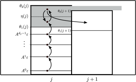
Figure 1: A typical lineage of individuals. The population makes progress keeping its $j$ leading 1-bits and raising mutation rate. Once in the edge region (grey), it remains in the edge region while increasing or decreasing mutation. Individuals in the edge region can move to a strictly better level by obtaining at least $j+1$ leading 1-bits and lowering mutation rate.

Fig. 1 illustrates a typical lineage of individuals, from fitness level $j$ to fitness level $j+1$. Starting from some low mutation rate in fitness level $j$, the mutation rate is increased by a factor of $A$ in each generation, until the mutation rate reaches the interval $[\theta_{1}(j),\theta_{2}(j)]$, i.e., the edge level. The lineage circulates within the edge level for some generations, crossing an intermediary value $\eta(j)$, before the fitness improves, and fitness level $j+1$ is reached.

It is critical to show that with sufficiently high probability, the lineage remains in the edge level before upgrading to fitness level $j+1$. This is ensured by the bounds in Lemma 3. Statement (vii) implies that we cannot overshoot the edge level by increasing the mutation rate. Statement (iv) implies that below the intermediary mutation rate $\eta(j)$, the mutation rate can still be increased by a factor of $A$. Conversely, statement (v) means that above the intermediary mutation rate $\eta(j)$, it is safe to decrease the mutation rate by a factor of $b$. Statements (viii) and (ix) ensure that an individual in an edge level can always either increase or decrease mutation rate for there to be a sufficiently high probability of maintaining the individual’s fitness value. Finally, statements (ii) and (iii) imply that within the edge level, the upgrade probability is $\Theta(1/j)$.

Before we can prove these statements, recall that we have delayed formally defining the functions $\theta_{1}$, $\eta$, or $\theta_{2}$. In order to derive the claimed bounds for Lemma 3, we do this now. For $j\geq 1$, let

$$\eta(j) :=\frac{1}{2A}\left(1-\left(\frac{1+\delta}{\alpha_{0}p_{\text{inc}}}\right)^{1/j}\right)$$ (13)

$$\theta_{1}(j) :=b\eta(j)$$ (14)

$$\theta_{2}(j) :=1-q^{1/j}$$ (15)

where

$$q:=\frac{1-\zeta}{\alpha_{0}},\quad r_{0}:=\frac{1+\delta}{\alpha_{0}(1-p_{\text{inc}})},\text{ and }$$

$$\zeta:=1-\alpha_{0}(r_{0})^{1+\sqrt{r_{0}}}.$$ (16)

Furthermore, for the special case $j=0$, define

$$\eta(0):=\frac{\eta(1)}{A},\quad\theta_{1}(0):=b\eta(0),\quad\text{and}\quad\theta_{2}(0):=\frac{\theta_{2}(1)}{b}.$$

Note that these definitions, along with statement (i) of Lemma 3, ensure $\theta_{1}$ and $\theta_{2}$ satisfy the informal conditions from Section 3.1 for $\varepsilon$ small enough.

Lemma 3.

Let $A>1$, $b<1$, and $p_{\text{inc}}\in(0,1)$ be constants satisfying the constraints in Theorem 2. Then there exists a constant $\delta\in(0,1/10)$ such that for all $j\in[0..k-1]$ and $\chi/n\in[\varepsilon,1/2]$,

1. $\theta_{1}(0)<\eta(0)<1/2<\theta_{2}(0)$,

2. $\theta_{2}(j)=\Omega(1/j)$

3. $\theta_{1}(j)=O(1/j)$

4. $A\eta(j)\leq\theta_{2}(j)$,

5. $b\eta(j)\geq\theta_{1}(j)$,

6. $b\theta_{2}(j)<\theta_{2}(j+1)$,

7. $A\theta_{1}(j)\leq\theta_{2}(j+1)$,

8. if $\frac{\chi}{n}\leq\eta(j),$ then $r(j,A\chi)\geq\frac{1+\delta}{\alpha_{0}p_{\text{inc}}}$, and

9. if $\frac{\chi}{n}\leq\theta_{2}(j)$, then $r(j,b\chi)\geq\frac{1+\delta}{\alpha_{0}(1-p_{\text{inc}})}$.

Proof.

Before proving statements (i)–(ix), we derive bounds on the three constants $q,\zeta,$ and $r_{0}$. By the assumptions $p_{\text{inc}}<2/5$ and $\alpha_{0}\geq 4$ from Theorem 2 and $\delta<1/10$,

$$r_{0}<\frac{11}{6\alpha_{0}}<1.$$ (17)

Furthermore, since $r_{0}<1$ and $\alpha_{0}\geq 4$, we have

$$\zeta >1-\alpha_{0}(r_{0})^{2}>1-\frac{1}{\alpha_{0}}\left(\frac{11}{6}\right)^{2}\geq\frac{23}{144}.$$ (18)

Finally, since $\delta,\zeta,p_{\text{inc}}\in(0,1)$, we have from the definitions of $r_{0}$ and $q$ that

$$0<q<r_{0}.$$ (19)

From the definition of the functions $\theta_{1}$, $\eta$, and the constant $\delta\in(0,1/10)$, it follows that

$$\theta_{1}(0) <\eta(0)<\eta(1)<\frac{1}{2A}\left(1-\frac{1}{\alpha_{0}p_{\text{inc}}}\right)<\frac{1}{2}.$$

Also, we have from the definition of $q$, the constraint $\alpha_{0}\geq 4$ from Theorem 2, and the bound $\zeta>23/144$ from (18) that

$$\theta_{2}(0) >\theta_{2}(1)>1-q=1-\frac{1-\zeta}{\alpha_{0}}>1-\frac{1-\frac{23}{144}}{4}=\frac{455}{576}.$$

Thus, we have proven statement (i).

Statement (ii) follows directly from Lemma 7, the definition of $\theta_{2}$ and the constant $q$,

$$\theta_{2}(j) =1-q^{1/j}\geq\ln(1/q)/j=\Omega(1/j).$$

For statement (iii), we define $c:=\frac{1+\delta}{\alpha_{0}p_{\text{inc}}}<1$, and observe that the inequality $e^{x}\geq 1+x$ implies

$$\theta_{1}(j)<1-c^{1/j}=1-e^{(1/j)\ln(c)}\leq-(1/j)\ln(c)=O(1/j).$$

For statement (iv), first note that Eq. (19) and the assumption $p_{\text{inc}}<2/5$ imply

$$0<q<r_{0}<\frac{1+\delta}{\alpha_{0}p_{\text{inc}}}.$$

For $j\geq 1$, we therefore have $1/j>0$ and

$$\theta_{2}(j)=1-q^{1/j}\geq 1-\left(\frac{1+\delta}{\alpha_{0}p_{\text{inc}}}\right)^{1/j}\geq A\eta(j).$$

For $j=0,$ the definition of $\eta(0)$, statement (iv) for the case $j=1$ shown above, and the definition of $\theta_{2}(0)$ give

$$A\eta(0) =\eta(1)\leq\frac{\theta_{2}(1)}{A}=\frac{b\theta_{2}(0)}{A}<\theta_{2}(0).$$

Statement (v) follows from the definition of $\theta_{1}(j)$.

We now show (vi). The statement is true by definition for $j=0$, so assume that $j\geq 1$. We first derive an upper bound on the parameter $b$ in terms of the constant $q$. In particular, the constraint on $b$ from Theorem 2 and the relationship $0<q<r_{0}$ from (19) give

$$b \leq\frac{1}{1+\sqrt{r_{0}}}<\frac{1}{1+\sqrt{q}}=\frac{1-\sqrt{q}}{1-q}.$$ (20)

The right hand side of (20) can be further bounded by observing that the function $g(j):=\frac{1-q^{1/(j+1)}}{1-q^{1/j}}$ with $q>0$ increases monotonically with respect to $j$. Thus, for all $j\in\mathbb{N}$, we have

$$b<\frac{1-\sqrt{q}}{1-q} \leq\frac{1-q^{1/(j+1)}}{1-q^{1/j}}.$$ (21)

This upper bound on parameter $b$ now immediately leads to the desired result

$$b\theta_{2}(j) =b(1-q^{1/j})\leq 1-q^{1/(j+1)}=\theta_{2}(j+1).$$ (22)

Statement (vii) follows by applying the previous three statements in the order (v), (iv), and (vi)

$$A\theta_{1}(j)\leq Ab\eta(j)\leq b\theta_{2}(j)\leq\theta_{2}(j+1).$$

Next we prove statement (viii). The statement is trivially true for $j=0$, because $r(0,A\chi)=1$, so assume that $j\geq 1$. By the assumption $\chi/n\leq\eta(j)$ and the definition of $\eta(j)$,

$$r(j,A\chi) =\left(1-\frac{A\chi}{n}\right)^{j}\geq\left(1-A\eta(j)\right)^{j}$$

$$\geq\left(1-\left(1-\left(\frac{1+\delta}{\alpha_{0}p_{\text{inc}}}\right)^{1/j}\right)\right)^{j}=\frac{1+\delta}{\alpha_{0}p_{\text{inc}}}.$$

Finally, we prove statement (ix). Again, the statement is trivially true for $j=0$, because $r(0,b\chi)=1$, so assume that $j\geq 1$. We derive an alternative upper bound on parameter $b$ in terms of $r_{0}$ and $q$. By the constraint on $b$ in Theorem 2,

$$b \leq\frac{1}{1+\sqrt{r_{0}}}=\frac{\ln(r_{0})}{\ln(r_{0})+\sqrt{r_{0}}\ln(r_{0})}$$

$$=\frac{\ln(r_{0})}{\ln\left(r_{0}r_{0}^{\sqrt{r_{0}}}\right)}=\frac{\ln r_{0}}{\ln q}.$$ (23)

Furthermore, note that the function $h(j):=\frac{1-r_{0}^{1/j}}{1-q^{1/j}}$ decreases monotonically with respect to $j$ when $r_{0}>q>0$, and has the limit $\lim_{j\rightarrow\infty}h(j)=\ln(r_{0})/\ln(q)$. Using (23), it therefore holds for all $j\in\mathbb{N}$ that

$$b\leq\frac{\ln r_{0}}{\ln q}\leq\frac{1-r_{0}^{1/j}}{1-q^{1/j}}.$$ (24)

The assumption $\chi/n\leq\theta_{2}(j)$, the definition of $\theta_{2}(j)$, and (24) now give

$$r(j,b\chi) =\left(1-\frac{b\chi}{n}\right)^{j}\geq\left(1-b\theta_{2}(j)\right)^{j}$$

$$=\left(1-b\left(1-q^{1/j}\right)\right)^{j}\geq\left(1-\left(1-r_{0}^{1/j}\right)\right)^{j}=r_{0},$$

which completes the proof of statement (ix). ∎

Using Lemma 3, we are now in a position to prove that the levels satisfy condition (G2). If the mutation rate $\chi/n$ is above the intermediary value $\eta(j)$, there is a sufficiently high probability of reducing the mutation rate while maintaining the fitness. Conversely, if the mutation rate is below the intermediary value $\eta(j)$, there is a sufficiently high probability of increasing the mutation rate while maintaining the fitness.

Lemma 4.

Assume that the parameters $A,b,$ and $p_{\text{inc}}$ satisfy the constraints in Theorem 2. Then there exists a constant $\delta\in(0,1/10)$ such that for all $j\in[0..k-1]$ and all $\ell\in[d_{j}]$, if Algorithm 1 in step 8 selects a parent $(x,\chi/n)\in A_{(j,\ell)}$, then the offspring $(x^{\prime},\chi^{\prime}/n)$ created in steps 9 and 10 of the algorithm satisfies

$$\operatorname*{Pr}\left((x^{\prime},\chi^{\prime}/n)\in A_{\geq(j,\ell)}\right)\geq\frac{1+\delta}{\alpha_{0}}.$$

Proof.

We will prove the stronger statement that with probability $(1+\delta)/\alpha_{0}$, we have simultaneously

$$x^{\prime}\in A_{\geq j}\quad\text{and}\quad\min\left\{\frac{\chi}{n},\theta_{1}(j)\right\}\leq\frac{\chi^{\prime}}{n}\leq\theta_{2}(j).$$ (25)

The event (25) is a subset of the event $(x^{\prime},\chi^{\prime}/n)\in A_{\geq(j,\ell)}$, because a lower level $A_{(j,\ell)}$ may contain search points $(x^{\prime},\chi^{\prime}/n)$ with mutation rates $\chi^{\prime}/n<\min(\chi/n,\theta_{1}(j))$.

By Definition 4, the parent satisfies $x\in A_{\geq j}$ and $\chi/n\leq\theta_{2}(j)$. We distinguish between two cases.

Case 1: $\chi/n\leq\eta(j)$. By Lemma 3 (i), and the monotonicity of $\eta$, we have $\eta(j)<1/2$. Note that in this case, it is still “safe” to increase the mutation rate. For a lower bound, we therefore pessimistically only account for offspring where the mutation parameter is increased from $\chi<n/2$ to $\min(A\chi,n/2)$. Note first that since $A>1,$ we have

$$\frac{\chi^{\prime}}{n}=\frac{\min(A\chi,n/2)}{n}>\frac{\chi}{n}.$$

Also, Lemma 3 (iv) implies the upper bound

$$\frac{\chi^{\prime}}{n}\leq\frac{A\chi}{n}\leq A\eta(j)\leq\theta_{2}(j).$$

To lower bound the probability that $x^{\prime}\in A_{\geq j}$, we consider the event where the mutation rate is increased, and the event that none of the first $j$ bits in the offspring are mutated with the new mutation parameter $\min(A\chi,n/2)$. By definition of the algorithm and using Lemma 3 (viii), these two events occur with probability at least

$$p_{\text{inc}}r(j,A\chi)\geq(1+\delta)/\alpha_{0}.$$ (26)

Case 2: $\eta(j)<\chi/n\leq\theta_{2}(j)$. Note that in this case, it may be “unsafe” to increase the mutation rate. For a lower bound, we pessimistically only consider mutation events where the mutation parameter is decreased from $\chi$ to $b\chi$. Analogously to above, since $b<1$, we have

$$\frac{\chi^{\prime}}{n}=\frac{b\chi}{n}<\frac{\chi}{n}\leq\theta_{2}(j).$$ (27)

Furthermore, Lemma 3 (v) implies the lower bound

$$\frac{\chi^{\prime}}{n}=\frac{b\chi}{n}>\frac{b\eta(j)}{n}\geq\theta_{1}(j).$$ (28)

To lower bound the probability that $x^{\prime}\in A_{\geq j}$, we consider the event where the mutation parameter is decreased from $\chi$ to $b\chi$, and the offspring $x^{\prime}$ is not downgraded to a lower level. By definition of the algorithm, $r(j,b\chi)$, and using Lemma 3 (ix), these two events occur with probability

$$(1-p_{\text{inc}})r(j,b\chi)\geq(1+\delta)/\alpha_{0}.$$ (29)

Hence, we have shown that in both cases, the event in Eq. (25) occurs with probability at least $(1+\delta)/\alpha_{0}$, which completes the proof. ∎

We now show that the edge levels satisfy condition (G1) of the level-based theorem. As we will show later, the upgrade probability for non-edge levels is constant.

Lemma 5.

Assume that the parameters $b$ and $p_{\text{inc}}$ satisfy the constraints in Theorem 2. Then for any $j\in[0..k-1]$, and any search point $(x,\chi/n)\in A_{(j,d_{j})}$ selected in step 8 of Algorithm 1 applied to $\textsc{LeadingOnes}_{k}$, the offspring $(x^{\prime},\chi^{\prime}/n)$ created in steps 9 and 10 satisfies $\operatorname*{Pr}\left((x^{\prime},\chi^{\prime}/n)\in A_{\geq(j+1,1)}\right)=\Omega(1/j).$

Proof.

By the definition of level $A_{(j,d_{j})}$, we have $\theta_{1}(j)\leq\chi/n\leq\theta_{2}(j)$ and so by Lemma 3 (vi), we have $b\chi/n\leq\theta_{2}(j+1)$. Given the definition of levels $A_{\geq(j+1,1)}$, it suffices for a lower bound to only consider the probability of producing an offspring $(x^{\prime},\chi^{\prime}/n)$ with lowered mutation rate $\chi^{\prime}/n=b\chi/n\leq\theta_{2}(j+1)$ and fitness $\textsc{LO}_{k}(x^{\prime})\geq j+1$.

We claim that if the mutation rate is lowered, the offspring has fitness $\textsc{LO}_{k}(x^{\prime})\geq j+1$ with probability $\Omega(1/j).$ Since the parent belongs to level $A_{(j,d_{j})}$, it has fitness $\textsc{LO}_{k}(x)\geq j$, so we need to estimate the probability of not flipping the first $j$ bits, and obtain a 1-bit in position $j+1$.

We now estimate the probability of obtaining a 1-bit in position $j+1$, assuming that the parent $x$ already has a 1-bit in this position, for any $j\in[0..k-1]$. Using that $\theta_{2}(j)$ decreases monotonically in $j$, the definition of $\theta_{2}(0)$, and the lower bound on the parameter $\zeta>23/144$ from Eq. (18), the probability of not mutating bit-position $j+1$ with the lowered mutation rate $b\chi/n$ is

$$1-\frac{b\chi}{n} \geq 1-b\theta_{2}(j)\geq 1-b\theta_{2}(0)$$

$$=1-\theta_{2}(1)=1-\frac{1-\zeta}{\alpha_{0}}>1-\frac{1-\frac{23}{144}}{\alpha_{0}}=\Omega(1).$$

If the parent $x$ does not have a 1-bit in position $j+1$, we need to flip this bit-position. By the definition of $\theta_{1}(j)$ in Eq. (14), the probability of this event is in the case $j\geq 1$

$$\frac{b\chi}{n} \geq b\theta_{1}(j)=\frac{b^{2}}{2A}\left(1-\left(\frac{1+\delta}{\alpha_{0}p_{\text{inc}}}\right)^{1/j}\right)$$ (30)

$$\geq\frac{b^{2}}{2Aj}\ln\left(\frac{\alpha_{0}p_{\text{inc}}}{1+\delta}\right)=\Omega(1/j),$$ (31)

where the last inequality follows from Lemma 7. If $j=0$, we use that $\theta_{1}(j)$ decreases monotonically in $j$ and Eqs. (30)–(31) to show that the probability of flipping bit $j+1=1$ is

$$\frac{b\chi}{n}\geq b\theta_{1}(0)>b\theta_{1}(1)=\Omega(1).$$

The claim that we obtain a 1-bit in position $j+1$ with probability $\Omega(1/j)$ is therefore true.

Thus, the probability of lowering the mutation rate to $b\chi/n$, obtaining a 1-bit in position $j+1$, and not flipping the first $j$ positions is, using the definition of $\theta_{2}(j)$ in (15),

$$(1-p_{\text{inc}})\Omega(1/j)\left(1-\frac{b\chi}{n}\right)^{j}\\ >\Omega(1/j)\left(1-\theta_{2}(j)\right)^{j}=\Omega(1/j)\left(\frac{1-\zeta}{\alpha_{0}}\right)=\Omega(1/j),$$

which completes the proof. ∎

3.3 Individuals with Too High Mutation Rates

Highly fit individuals with incorrect parameter settings can cause problems for self-adaptive EAs. If there are too many such “bad” individuals in the population, they may dominate the population, propagate bad parameter settings, and thus impede progress. In this section, we therefore bound the number of such bad individuals. We define a region $B\subset\mathcal{Y}$ containing search points with a mutation rate that is too high relative to their fitness. For the constant $\zeta\in(0,1)$ defined in Eq. (16), let

$$B :=\Big{\{}(x,\chi/n)\in A_{j}\times[\varepsilon,1/2]\mid$$ (32)

$$\quad j\in\mathbb{N}_{0}\;\wedge\;\forall y\in\mathcal{X}\operatorname*{Pr}_{x^{\prime}\sim p_{\text{mut}}(y,\chi)}(x^{\prime}\in A_{\geq j})<\frac{1-\zeta}{\alpha_{0}}\Big{\}}.$$

Note that by the definition of the function $\theta_{2}(j)$, it holds for all $y\in\mathcal{X}$ that the statement $\operatorname*{Pr}_{x^{\prime}\sim p_{\text{mut}}(y,\chi)}(x^{\prime}\in A_{\geq j})=(1-\chi/n)^{j}<(1-\zeta)/\alpha_{0}$ is analogous to $\chi/n>\theta_{2}(j)$. Therefore, the region $B$ can also be expressed as

$$B=\bigcup_{j=0}^{k-1}A_{>j}\times\left(\min\left(\frac{1}{2},\theta_{2}(j+1)\right),\min\left(\frac{1}{2},\theta_{2}(j)\right)\right].$$ (33)

An individual $(x,\chi/n)\in B$ is said to have too high mutation rate. To see why, recall that the number of offspring of $(x,\chi/n)$ is never more than $\alpha_{0}$. Since the probability an offspring has fitness as least as good as $f_{k}(x)$ is less than $1/\alpha_{0}$, in expectation less than one offspring maintains the fitness, making it unlikely a lineage of $(x,\chi/n)$ will be able to make progress towards the optimum. This corresponds to the “error threshold” discussed in [29]; by Corollary 1 in [29], the probability that a group of individuals of size $\text{poly}(k)$ staying in $B$ will optimise $\textsc{LO}_{k}$ in sub-exponential time is $e^{-\Omega(k)}$.

The levels given by Definition 4 are not disjoint from the region $B$ defined above. This is an important departure from the approach used in [8], where $B$ is effectively removed from the search space and the level-based theorem is applied to a partition over $\mathcal{Y}\setminus B$. This is not effective in our setting, since an individual can have a sudden increase in fitness but can not significantly decrease mutation rate. Such an individual may have too high mutation rate with respect to its new fitness, but we still depend on this individual having correctly tuned mutation with respect to the old fitness value. Therefore, an individual in some $A_{(j,\ell)}$ may mutate in and out of $B$ before its mutation rate has been adapted to maintain a fitness higher than $j$. While individuals may occasionally jump into the bad region, if too many individuals are in $B$ at a given time this may destroy the progress of the algorithm. In particular, if $|P_{t}\cap B|>\mu$, then assuming all individuals in $B$ have strictly better fitness and higher mutation rate than those not in $B$, only individuals from $B$ will be selected for mutation and the next generation will consist only of individuals with very high mutation rate. Therefore, it is critical that for any generation $t\in\mathbb{N}$, the number of individuals in $B$ will be less than $\mu$ with overwhelmingly high probability. We prove this with the following lemma, which is similar to Lemma 2 from [8], but with the notable difference that the size of $B$ can be controlled within a single generation, regardless the configuration of $P_{t-1}$.

Lemma 6.

Let $B\subseteq\mathcal{Y}$ be as defined in Eq. (32) for a constant $\zeta\in(0,1)$. Then for any generation $t\in\mathbb{N}$ of Algorithm 1 applied to $\textsc{LeadingOnes}_{k}$,

$$\operatorname*{Pr}(|B\cap P_{t}|\geq(1-\zeta/2)\mu)\leq e^{-\Omega(\mu)}.$$

Proof.

Consider some parent $(x,\chi/n)$ selected in generation $t-1\geq 0$ and step 8 of Algorithm 1. Referring to steps 9 and 10, first a new mutation parameter $\chi^{\prime}$ is chosen, then a new bitstring $x^{\prime}$ is obtained from $x$ using bitwise mutation with mutation parameter $\chi^{\prime}$. To obtain an upper bound on the probability that $(x^{\prime},\chi^{\prime}/n)$ is in $B$, we proceed in cases based on the outcome of sampling $\chi^{\prime}$, namely, whether the chromosome $(x,\chi^{\prime}/n)$ is in $B$.

If $(x,\chi^{\prime}/n)\in B$: then it follows immediately from the definition of $B$ that independently of the chosen parent $x$, it holds

$$\Pr\left((x^{\prime},\chi^{\prime}/n)\in B\right)<\frac{1-\zeta}{\alpha_{0}}.$$ (34)

If $(x,\chi^{\prime}/n)\not\in B$: then for $(x^{\prime},\chi^{\prime}/n)$ to end up in $B$, by Eq. (33) it is necessary that $x^{\prime}\in A_{\geq u}$ for some $u>j$, where $x\in A_{j}$ and $r(u,\chi^{\prime})<(1-\zeta)/\alpha_{0}$. Since $\chi^{\prime}/n<1/2$, the probability of obtaining $x^{\prime}\in A_{\geq u}$ is no more than

$$\left(1-\frac{\chi^{\prime}}{n}\right)^{u-1}\left(\frac{\chi^{\prime}}{n}\right)<\left(1-\frac{\chi^{\prime}}{n}\right)^{u}<\frac{1-\zeta}{\alpha_{0}}.$$ (35)

Since each of the $\lambda$ individuals in population $P_{t}$ are sampled independently and identically, Eqs. (34) and (35) imply $|B\cap P_{t}|$ is stochastically dominated by a binomially distributed random variable $Z\sim\operatorname*{Bin}(\lambda,\tfrac{1-\zeta}{\alpha_{0}})$ which has expectation $\mu(1-\zeta)$. By a Chernoff bound,

$$\Pr\left(|B\cap P_{t}|\geq\mu(1-\zeta/2)\right)\leq\Pr\left(Z\geq\mu(1-\zeta/2)\right)$$

$$=\Pr\left(Z\geq E\left[Z\right]\left(1+\tfrac{1}{2(1-\zeta)}\right)\right)=e^{-\Omega(\mu)}.$$

∎

3.4 Applying the Level-based Theorem

We now combine the results of Sections 3.1, 3.2, and 3.3 to prove Theorem 2 using Theorem 1.

Proof (of Theorem 2).

We partition the search space $\mathcal{Y}$ into the sets $A_{(j,\ell)}$ from Definition 4, where $j\in[0..k-1]$ and $\ell\in[d_{j}]$, along with $A_{(k,1)}$, and define $A_{\geq(j,\ell)}$ as in (12).

We say that a generation $t$ is “failed” if the population $P_{t}$ contains more than $(1-\zeta/2)\mu$ individuals in region $B$. First, we will optimistically assume that no generations fail. Under this assumption, we will prove that the conditions of Theorem 1 hold, leading to an upper bound on the expected number of function evaluations $t_{0}(k)$ until a search point in $A_{(k,1)}$ is created (i.e. a global optimum is found). Then in the end we will use a restart argument to account for failed generations.

Let $\gamma_{0}:=(\zeta/2)(\mu/\lambda)$. In the following arguments, we will make consistent use of the important fact that for $\gamma\in(0,\gamma_{0}]$, if there are $\gamma\lambda$ individuals in levels $A_{\geq(j,\ell)}$ for some $j\in\{0,\dots,k-1\}$ and $\ell\in[d_{j}]$, then the probability of selecting an individual from $A_{\geq(j,\ell)}$ is $\gamma\alpha_{0}$. To see this, we note that individuals in $A_{\geq(j,\ell)}$ are guaranteed to be ranked above those in $\mathcal{Y}\setminus\left(A_{\geq(j,\ell)}\cup B\right)$ in line 6 of Algorithm 1, since individuals in $\mathcal{Y}\setminus\left(A_{\geq(j,\ell)}\cup B\right)$ must have fitness either strictly less than $j$, or equal to $j$, and hence have mutation rate too low to be contained in $A_{\geq(j,\ell)}$. Recalling that $|P_{t}\cap B|\leq(1-\zeta/2)\mu$, it follows that all $\gamma\lambda\leq(\zeta/2)\mu$ individuals of $A_{\geq(j,\ell)}$ are among the $\mu$ fittest in the population. Therefore, the probability of selecting an individual from $A_{\geq(j,\ell)}$ indeed is $\gamma\lambda/\mu=\gamma\alpha_{0}$.

We now show that conditions (G1) and (G2) of Theorem 1 hold for each level $A_{(j,\ell)}$ where $j\in[0..k-1]$ and $\ell\in[d_{j}]$. We assume that the current population has at least $\gamma_{0}\lambda$ individuals in levels $A_{\geq(j,\ell)}$. We distinguish between the case $\ell<d_{j}$, i.e., when it suffices to increase the mutation rate to upgrade to the next level, and the case $\ell=d_{j}$, i.e., when it may be necessary to increase the fitness to reach the next level.

$\ell<d_{j}$: To verify condition (G2), we must estimate the probability of producing an offspring in levels $A_{\geq(j,\ell+1)}$, assuming that there are at least $\gamma\lambda$ individuals in levels $A_{\geq(j,\ell+1)}$, for any $\gamma\in(0,\gamma_{0}]$. To produce an offspring in levels $A_{\geq(j,\ell+1)}$, it suffices to first select a parent $(x,\chi/n)$ from $A_{\geq(j,\ell+1)}$, and secondly create an offspring $(x^{\prime},\chi^{\prime}/n)$ in levels $A_{\geq(j,\ell+1)}$. The probability of selecting such a parent is at least $\gamma\alpha_{0}$. Assuming that the parent is in level $A_{(u,v)}\subseteq A_{\geq(j,\ell+1)}$, and applying Lemma 4 to level $A_{(u,v)}$, the probability that the offspring $(x^{\prime},\chi^{\prime}/n)$ is in levels $A_{\geq(u,v)}\subseteq A_{\geq(j,\ell+1)}$ is $(1+\delta)/\alpha_{0}$ for some $\delta\in(0,1)$. Thus the probability of selecting a parent in levels $A_{\geq(j,\ell+1)}$, then producing an offspring in levels $A_{\geq(j,\ell+1)}$, is at least $\gamma\alpha_{0}\left(\frac{1+\delta}{\alpha_{0}}\right)=\gamma(1+\delta)$, so condition (G2) is satisfied.

To verify condition (G1), we estimate the probability of producing an offspring in levels $A_{\geq(j,\ell+1)}$. If the parent is in levels $A_{\geq(j,\ell+1)}$, then again by Lemma 4, the offspring is in levels $A_{\geq(j,\ell+1)}$ with probability at least $(1+\delta)/\alpha_{0}$.

On the other hand, if the parent $(x,\chi/n)$ is in level $A_{(j,\ell)}$, then we consider the probability of producing an offspring $(x^{\prime},\chi^{\prime}/n)\in A_{\geq(j,\ell+1)}$ by increasing the mutation rate from $\chi$ to $A\chi$, and maintaining the fitness $x^{\prime}\in A_{\geq j}$. By assumption, $\ell<d_{j}$, so the level-definition implies that the parent has mutation rate $\chi/n<\theta_{1}(j)<\eta(j)$. Hence, by Lemma 3 (viii), the probability of increasing the mutation parameter to $A\chi$ and maintaining at least $j$ leading one-bits is at least $p_{\text{inc}}r(j,A\chi)\geq(1+\delta)/\alpha_{0}.$

Taking into account that the probability of selecting a parent in $A_{\geq(j,\ell)}$ is at least $\alpha_{0}\gamma_{0}$, the probability of producing an offspring in $A_{\geq(j,\ell+1)}$ is at least

$$\gamma_{0}\alpha_{0}\left(\frac{1+\delta}{\alpha_{0}}\right) =(1+\delta)\gamma_{0}=:z_{(j,\ell)}.$$ (36)

$\ell=d_{j}$: To show (G2) we assume that there are at least $\gamma\lambda$ individuals in levels $A_{\geq(j+1,1)}$, for $\gamma\in(0,\gamma_{0}]$. We again apply Lemma 4 to show the probability of selecting an individual from $A_{\geq(j+1,1)}$ and producing a new individual also in $A_{\geq(j+1,1)}$ is at least $\gamma(1+\delta)$, showing (G2) is satisfied.

For condition (G1), we only consider parents selected from levels $A_{\geq(j+1,1)}$. If the parent $(x,\chi/n)$ is in $A_{(j,d_{j})}$, then by Lemma 5 the offspring $(x^{\prime},\chi^{\prime}/n)$ is in levels $A_{\geq(j+1,1)}$ with probability at least $\Omega(1/j)$. Otherwise, if the parent is already in levels $A_{\geq(j+1,1)}$, then by Lemma 4, the offspring is in levels $A_{\geq(j+1,1)}$ with probability at least $(1+\delta)/\alpha_{0}=\Omega(1)$. In both cases, the probability of selecting a parent from $A_{\geq(j,d_{j})}$ and producing an offspring in levels $A_{\geq(j+1,1)}$ is at least

$$\gamma_{0}\alpha_{0}\Omega(1/j)=\Omega(1/j)=:z_{(j,d_{j})}.$$ (37)

To verify that $\lambda\geq c\ln(n)$ is large enough to satisfy condition (G3), we first must calculate $m$, the total number of sub-levels. Referring to Definition 3 and using $\theta_{1}(j)<1/2$, the depth of each level $j$ is no more than $d_{j}<\lceil\log_{A}\left(\frac{1}{2\varepsilon}\right)\rceil=O(\log(n))$ for all $j\in\{0,\dots,k-1\}$. Therefore, $m=O(k\log(n))$ and so $\lambda\geq c\ln(n)$ satisfies (G3) for $c>1$ large enough. Thus we have found parameters $z_{(0,1)},z_{(0,2)},\dots,z_{(k-1,d_{k-1})},\delta,$ and $\gamma_{0},$ such that all three conditions of Theorem 1 are satisfied. Assuming no failure, the expected time to reach the last level is no more than

$$t_{0}(k) \leq\left(\frac{8}{\delta^{2}}\right)\sum_{j=0}^{k-1}\sum_{\ell=1}^{d_{j}}\left(\lambda\log\left(\frac{6\delta\lambda}{4+z_{(j,\ell)}\delta\lambda}\right)+\frac{1}{z_{(j,\ell)}}\right)$$

$$=\sum_{j=0}^{k-1}\sum_{\ell=1}^{d_{j}-1}O\left(\lambda\log\left(\frac{1}{z_{(j,\ell)}}\right)+\frac{1}{z_{(j,\ell)}}\right)$$

$$\quad+\sum_{j=0}^{k-1}O\left(\lambda\log(\lambda)+\frac{1}{z_{(j,d_{j})}}\right)$$

$$=O(k\lambda\log(n)+k\lambda\log(\lambda)+k^{2}),$$

using that $z_{(j,\ell)}=\Omega(1)$ for all $\ell<d_{j}$, and $z_{(j,d_{j})}=\Omega(1/j)$.

Finally, we account for “failed” generations where our assumption that there are less than $(1-\zeta/2)\mu$ individuals in region $B$ does not hold. We refer to a sequence of $2t_{0}(k)/\lambda$ generations as a phase, and call a phase good if for $2t_{0}(k)/\lambda$ consecutive generations there are fewer than $(1-\zeta/2)\mu$ individuals in $B$. By Lemma 6 and a union bound, a phase is good with probability $1-2t_{0}(k)/\lambda e^{-\Omega(\mu)}=\Omega(1)$, for $\mu=\Omega(\log(n))$. By Markov’s inequality, the probability of reaching a global optimum in a good phase is at least $1/2$. Hence, the expected number of phases required, each costing $2t_{0}(k)$ function evaluations, is $O(1)$. ∎

4 Experiments

The theoretical analysis of the $(\mu,\lambda)$ self-adaptive EA is complemented by some experiments on a wider variety of problems. In addition to the standard OneMax function, we consider

$$\textsc{Jump}_{k}(x) :=\begin{cases}\textsc{OM}(x)+k&\text{if }\textsc{OM}(x)<n-k\\ \textsc{OM}(x)-k&\text{if }n-k\leq\textsc{OM}(x)<n\\ n+1&\text{if }\textsc{OM}(x)=n.\end{cases}$$

$$\textsc{SubString}_{k}(x) :=\max_{1\leq i\leq n}i\cdot\textstyle\prod_{j=\max\{i-k+1,1\}}^{i}x_{j}.$$

The $\textsc{SubString}_{k}$ function is similar to the function in [6] of the same name. The value of $\textsc{SubString}_{k}$ is the maximal position of the substring $1^{k}$, if such a substring exists, otherwise it is just the number of leading 1-bits. While the function in [6] has a unique global optimum at the point $1^{n}$, all strings of the form $\{0,1\}^{n-k}1^{k}$ are optimal for our $\textsc{SubString}_{k}$ function.

In a first set of experiments, we examined how Algorithm 1 adjusts mutation rates relative to fitness on several contrasting fitness landscapes. In each run, we chose the parameter settings $\lambda=8\ln(n)$, $\mu=\lambda/15$, $A=1.5$, $b=0.7$, and $p_{\text{inc}}=0.25$, where $\lambda$ and $\mu$ are rounded to the nearest integer. For the functions LeadingOnes, $\textsc{SubString}_{\sqrt{n}}$, OneMax, and $\textsc{Jump}_{3}$, we recorded the fitness and mutation rate $\chi/n$ of the top-ranked individual in each generation. In a second set of experiments, we compared Algorithm 1 to other algorithms on $\textsc{LeadingOnes}_{k}$, $\textsc{SubString}_{k}$, and a version of OneMax in which only an unknown selection of $k$ bits contribute to fitness ($\textsc{OneMax}_{k}$). For these experiments, we chose the parameters $\lambda=16\ln(n),$ $\mu=\lambda/8,$ $A=1.2,$ $b=0.7,$ $p_{\text{inc}}=0.25$ for Algorithm 1. The change in parameter settings was not particularly motivated, although note that both respect the conditions imposed by Theorems 2, since $p_{\text{inc}}=0.25$ satisfies $1/16<1/15<1/4<2/5$, and $b=0.7$ satisfies $7/10<1/(1+\sqrt{4/45})\approx 0.78$.

The results from the first set of experiments are summarised in Fig. 2. We set $n=500$ for LeadingOnes, $\textsc{SubString}_{\sqrt{n}}$, and OneMax, while for $\textsc{Jump}_{3}$ we set $n=100$, and performed 100 trials for each function. At the beginning of a trial, all individuals were given a starting mutation strength of $\chi=1$. For each function, we plotted the median mutation rate $\chi/n$ per fitness value in blue, with the 95th percentile shaded in grey. Finally, to aid interpretation we plotted in red the “error threshold”, i.e. the value of $\chi/n$ such that the expected number of offspring with fitness at least as good as the parent’s is only 1 [29]. For LeadingOnes, the error threshold is thus approximately the $\theta_{2}$ function introduced in Section 3.1.

Fig. 2 shows that Algorithm 1 tuned the mutation rate of the top-ranked individual very differently depending on the fitness landscape. For LeadingOnes, we see the top individual’s mutation rate quickly rose to a small factor below $\theta_{2}$, then gradually lowered mutation rate as fitness increased. This supports our theoretical analysis of $\textsc{LeadingOnes}_{k}$, in which we argued that the mutation rate rises to an “edge region” comprising of mutation rates just below the error threshold. We found similar behaviour for $\textsc{SubString}_{\sqrt{n}}$, where again the algorithm quickly rose to a close approximation below the error threshold. However, the results for OneMax and $\textsc{Jump}_{3}$ are less conclusive. First, we were unable to derive an exact expression for the error threshold for these functions, which makes the trajectory of the mutation rates more difficult to interpret. Instead we include in green the mutation rate for a single individual to maximise the expected difference in its fitness before and after mutation, in order to provide some context for interpreting the effectiveness of mutation rates. For OneMax, it is known this drift-maximising rate is $\Theta(1/n)$ when $\textsc{OM}(x)\geq 2n/3$ [18], while for $\textsc{Jump}_{3}$, the ideal rate is $3/n$ for jumping the gap. In terms of the trajectory of mutation rates, on OneMax the algorithm correctly increased its mutation rate at first, but also seems to have kept mutation rate well above $1/n$ for much of the search process. This could explain its relative inefficiency on $\textsc{OneMax}_{k}$ in the next set of experiments. The behaviour is similar for $\textsc{Jump}_{3}$, except that mutation rate increased toward the ideal rate while at the edge of the gap, and occasionally reached even higher values. The tendency for mutation rate to dramatically increase during lack of progress is reassuring, since a common difficulty in self-adaptation of mutation rates is that mutation rates may indefinitely decrease when it is difficult to increase fitness [35].

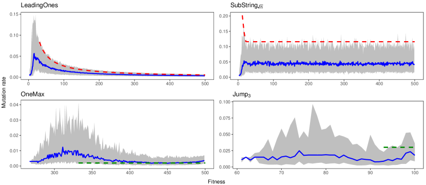
Figure 2: Fitness and mutation rate of the most fit individual per generation of Algorithm 1 with $\lambda=8\ln(n)$, $\mu=\lambda/15$, $A=1.5$, $b=0.7$, and $p_{\text{inc}}=0.25$. Median mutation rate is the blue line, while the 95-th percentile is shaded grey. Top: the dashed red line indicates the error threshold, past which mutation rates will be ineffective for the given fitness. Bottom: the dashed green line shows the drift-maximising mutation rate.

Figure 3: Runtime as a function of $k$ for fixed $n=2000$, normalised to show impact of adaptation. Points show the median runtime, with error bars extending beyond the interquartile range as $\pm 1.5\cdot\text{IQR}$. Parameter settings: Algorithm 1 with $\lambda=16\ln(n),\mu=2\ln(n),$ adaptation parameters $A=1.2,b=0.7,p_{\text{inc}}=0.25$. $(1+1)$ EA with mutation rate $1/n$. $(1+1)$ EA_α with $A=1.2$ and $b=0.85$. $(\mu,\lambda)$ EA with $\lambda=16\ln(n),\mu=2\ln(n)$ mutation rate $2/(5n)$.

In the second set of experiments, summarised in Fig. 3, we compared the self-adaptive EA to the $(1+1)$ EA, the $(\mu,\lambda)$ EA, as well as to the $(1+1)_{\alpha}$ EA from [23] with the parameter settings $A=1.2$ and $b=0.85$ (for the $(1+1)_{\alpha}$ EA). On each of the functions $\textsc{LeadingOnes}_{k}$, $\textsc{SubString}_{k}$, and $\textsc{OneMax}_{k}$, we tested the algorithms on a range of possible choices for the adversary by performing 100 runs of each algorithm for values of $k$ between $100$ and $n=2000$. The y-axes in Fig. 3 show the runtime divided by the asymptotic running time of a $(1+1)$ EA which knows the value $k$ beforehand. The effect of this rescaling is that algorithms which successfully adapt to the parameter $k$ should remain relatively constant along the y-axis as $k$ changes.

On all three functions, the two adaptive algorithms had runtimes proportional to an EA which knew $k$ beforehand. However, while both also drastically outperformed the static algorithms for smaller $k$ on $\textsc{LeadingOnes}_{k}$ and $\textsc{SubString}_{k}$, on $\textsc{OneMax}_{k}$, Algorithm 1 performed comparably to the static $(1+1)$ EA only for small $k$, and did worse than the $(1+1)$ EA as $k$ grew larger. This is somewhat expected, since it is known that the $(1+1)$ EA easily outperforms many population-based algorithms on OneMax. It is possible that the benefits of adaptation will not overcome the penalty of maintaining a population except for much larger values of $n$.

5 Conclusion

Effective parameter control is one of the central challenges in evolutionary computation. There is empirical evidence that self-adaptation – where parameters are encoded in the chromosome of individuals – can be a successful control mechanism in evolutionary strategies. However, self-adaptation is rarely employed in discrete EAs [1, 36]. The theoretical understanding of self-adaptation is lacking.

This paper demonstrates both theoretically and empirically that adopting a self-adaptation mechanism in a discrete, non-elitist EA can lead to significant speedups. We analysed the expected runtime of the $(\mu,\lambda)$ EA with self-adaptive mutation rates on $\textsc{LeadingOnes}_{k}$ in the context of an adversarial choice of a hidden problem parameter $k$ that determines the problem structure. We gave parameter settings for which the algorithm optimises $\textsc{LeadingOnes}_{k}$ in expected time $O(k^{2})$, which is asymptotically optimal among any unary unbiased black box algorithm which knows the hidden value $k$. This is a significant speedup compared to, e.g., the (1+1) EA using any choice of static mutation rate. In fact, the algorithm even has an asymptotic speedup compared with the state-of-the art parameter control mechanism for this problem [16]. Future work should extend the analysis to more general classes of problems, such as linear functions and multi-modal problems. We expect that applying the level-based theorem over a two-dimensional level-structure will lead to further results about self-adaptive EAs.

6 Appendix

Lemma 7.

For all $c>0$ and $j>0$, $1-c^{1/j}\geq\ln(1/c)/j.$

Proof.

$-\frac{1}{j}\ln(1/c)=\ln\left(c^{1/j}\right)\leq c^{1/j}-1.$ ∎

Acknowledgements

The authors would like to thank Dr Duc-Cuong Dang for suggesting the problem of determining the runtime of a self-adaptive evolutionary algorithm on the $\textsc{LeadingOnes}_{k}$ problem.

References

- [1] T. Bäck. Self-adaptation in genetic algorithms. In Proc. of the 1st European Conf on Artificial Life, pages 263–271, 1992.
- [2] T. Bäck and M. Schütz. Intelligent mutation rate control in canonical genetic algorithms. In Foundations of Intelligent Systems, pages 158–167, 1996.
- [3] G. Badkobeh, P. K. Lehre, and D. Sudholt. Unbiased black-box complexity of parallel search. In Proc. of Parallel Problem Solving from Nature (PPSN ’14), pages 892–901, 2014.
- [4] S. Böttcher, B. Doerr, and F. Neumann. Optimal fixed and adaptive mutation rates for the leadingones problem. In Proc. of Parallel Problem Solving from Nature (PPSN ’10), pages 1–10, 2010.
- [5] S. Cathabard, P. Lehre, and X. Yao. Non-uniform mutation rates for problems with unknown solution lengths. In Proc. of Foundations of Genetic Algorithms (FOGA ’11), pages 173–180, 2011.
- [6] T. Chen, P. K. Lehre, K. Tang, and X. Yao. When is an estimation of distribution algorithm better than an evolutionary algorithm? In Proc. of IEEE Congress on Evolutionary Computation, pages 1470–1477, 2009.
- [7] D. Corus, D.-C. Dang, A. V. Eremeev, and P. K. Lehre. Level-based analysis of genetic algorithms and other search processes. IEEE Transactions on Evolutionary Compututation, 22(5):707–719, 2017.
- [8] D.-C. Dang and P. K. Lehre. Self-adaptation of mutation rates in non-elitist populations. In Proc. of Parallel Problem Solving from Nature (PPSN ’16), pages 803–813, 2016.
- [9] D.-C. Dang, P. K. Lehre, and P. T. H. Nguyen. Level-based analysis of the univariate marginal distribution algorithm. Algorithmica, 81(2):668–702, 2019.
- [10] K. De Jong. A Historical Perspective. In Evolutionary Computation: a Unified Approach, chapter 2. MIT Press, Cambridge, 1st edition, 2006.
- [11] B. Doerr and C. Doerr. Optimal parameter choices through self-adjustment: Applying the 1/5-th rule in discrete settings. In Proc. of Genetic and Evolutionary Computation Conference (GECCO ’15), pages 1335–1342, 2015.
- [12] B. Doerr and C. Doerr. Optimal static and self-adjusting parameter choices for the (1+(, )) genetic algorithm. Algorithmica, 80(5):1658–1709, 2018.
- [13] B. Doerr and C. Doerr. Theory of parameter control for discrete black-box optimization: Provable performance gains through dynamic parameter choices. CoRR, abs/1804.05650, 2018.
- [14] B. Doerr, C. Doerr, and F. Ebel. From black-box complexity to designing new genetic algorithms. Theoretical Computer Science, 567:87 – 104, 2015.
- [15] B. Doerr, C. Doerr, and T. Kötzing. Unknown solution length problems with no asymptotically optimal run time. In Proc. of Genetic and Evolutionary Computation Conference (GECCO ’17), pages 1367–1374, 2017.
- [16] B. Doerr, C. Doerr, and T. Kötzing. Solving problems with unknown solution length at almost no extra cost. Algorithmica, 81(2):703–748, 2019.
- [17] B. Doerr, C. Doerr, and J. Lengler. Self-adjusting mutation rates with provably optimal success rules. In Proc. of Genetic and Evolutionary Computation Conference (GECCO ’19), pages 1479–1487, 2019.
- [18] B. Doerr, C. Doerr, and J. Yang. Optimal parameter choices via precise black-box analysis. In Proc. of Genetic and Evolutionary Computation Conference (GECCO ’16), pages 1123–1130, 2018.
- [19] B. Doerr, C. Gießen, C. Witt, and J. Yang. The (1+) evolutionary algorithm with self-adjusting mutation rate. In Proc. of Genetic and Evolutionary Computation Conference (GECCO ’17), pages 1351–1358, 2017.
- [20] B. Doerr, T. Jansen, D. Sudholt, C. Winzen, and C. Zarges. Mutation rate matters even when optimizing monotonic functions. Evolutionary Computation, 21(1):1–27, 2013.
- [21] B. Doerr, C. Witt, and J. Yang. Runtime analysis for self-adaptive mutation rates. In Proc. of Genetic and Evolutionary Computation Conference (GECCO ’18), pages 1475–1482, 2018.
- [22] C. Doerr. Complexity theory for discrete black-box optimization heuristics. CoRR, abs/1801.02037, 2018.
- [23] C. Doerr and M. Wagner. Simple on-the-fly parameter selection mechanisms for two classical discrete black-box optimization benchmark problems. In Proc. of Genetic and Evolutionary Computation Conference (GECCO ’18), pages 943–950, 2018.
- [24] S. Droste, T. Jansen, and I. Wegener. Dynamic parameter control in simple evolutionary algorithms. In Proc. of Foundations of Genetic Algorithms (FOGA ’01), pages 275 – 294, 2001.
- [25] A. E. Eiben, R. Hinterding, and Z. Michalewicz. Parameter control in evolutionary algorithms. IEEE Transactions on Evolutionary Computation, 3(2):124–141, 1999.
- [26] H. Einarsson, J. Lengler, M. M. Gauy, F. Meier, A. Mujika, A. Steger, and F. Weissenberger. The linear hidden subset problem for the (1 + 1) ea with scheduled and adaptive mutation rates. In Proc. of Genetic and Evolutionary Computation Conference (GECCO ’18), pages 1491–1498, 2018.
- [27] G. Karafotias, M. Hoogendoorn, and A. E. Eiben. Parameter control in evolutionary algorithms: Trends and challenges. IEEE Transactions on Evolutionary Computation, 19(2):167–187, 2015.
- [28] J. Lässig and D. Sudholt. Adaptive population models for offspring populations and parallel evolutionary algorithms. In Proc. of Foundations of Genetic Algorithms (FOGA ’11), pages 181–192, 2011.
- [29] P. K. Lehre. Negative drift in populations. In Proc. of Parallel Problem Solving from Nature (PPSN ’10), pages 244–253, 2010.
- [30] P. K. Lehre. Fitness-levels for non-elitist populations. In Proc. of Genetic and Evolutionary Computation Conference (GECCO ’11), pages 2075–2082, 2011.
- [31] P. K. Lehre and E. Özcan. A runtime analysis of simple hyper-heuristics: To mix or not to mix operators. In Proc of Foundations of Genetic Algorithms (FOGA ’13), pages 97–104, 2013.
- [32] P. K. Lehre and C. Witt. Black-Box Search by Unbiased Variation. Algorithmica, 64(4):623–642, 2012.
- [33] P. K. Lehre and X. Yao. On the impact of mutation-selection balance on the runtime of evolutionary algorithms. IEEE Transactions on Evolutionary Computation, 16(2):225–241, 2012.
- [34] J. Lengler. A general dichotomy of evolutionary algorithms on monotone functions. In Proc. of Parallel Problem Solving from Nature (PPSN ’18), pages 3–15, 2018.
- [35] K.-H. Liang, X. Yao, and C. Newton. Adapting self-adaptive parameters in evolutionary algorithms. Applied Intelligence, 15(3):171–180, 2001.
- [36] J. Smith and T. C. Fogarty. Self adaptation of mutation rates in a steady state genetic algorithm. In Proc. of IEEE International Conference on Evolutionary Computation, pages 318–323, 1996.
- [37] I. Wegener. Simulated annealing beats metropolis in combinatorial optimization. In Proc. of International Colloquium on Automata, Languages and Programming (ICALP ’05), pages 589–601, 2005.