Dislocations in a layered elastic medium with applications to fault detection

Abstract.

We consider a model for elastic dislocations in geophysics. We model a portion of the Earth’s crust as a bounded, inhomogeneous elastic body with a buried fault surface, along which slip occurs. We prove well-posedness of the resulting mixed-boundary-value-transmission problem, assuming only bounded elastic moduli. We establish uniqueness in the inverse problem of determining the fault surface and the slip from a unique measurement of the displacement on an open patch at the surface, assuming in addition that the Earth’s crust is an isotropic, layered medium with Lamé coefficients piecewise Lipschitz on a known partition and that the fault surface is a graph with respect to an arbitrary coordinate system. These results substantially extend those of the authors in Arch. Ration. Mech. Anal. 263 (2020), n. 1, 71–111.

1. Introduction

The focus of this work is an analysis of both the forward or direct problem, as well as the inverse problem, for a model of buried faults in the Earth’s crust. Specifically, we prove well-posedness of the direct problem, assuming only $L^{\infty}$ elastic coefficients, and uniqueness in the inverse problem, under additional assumptions, which are motivated by the ill-posedness of the inverse problem and are not overly restrictive for the applications we are concerned about.

We model the Earth’s crust as a layered, inhomogeneous elastic medium, and the fault as an oriented, open surface $S$ immersed in this elastic medium and not reaching the surface (the case of buried faults), along which there can be slippage of the rock. Faults can have any orientation with respect to the surface: horizontal, vertical, or oblique. When slip occurs, we speak of elastic dislocations. Mathematically, the slip is given by a non-trivial jump in the elastic displacement across the fault, represented by a non-zero vector field $\bm{g}$ on $S$. The surface of the Earth can be assumed traction free, that is, no load is bearing on it, while on the fault itself one can assume that the jump in the traction is zero, that is, the loads on the two sides of the fault balances out. (We refer the reader to [13, 15] for instance for a mathematical treatment of elasticity.)

The direct or forward problem consists in finding the elastic displacement in the Earth’s crust induced by the slip on the fault. The inverse problem consists in determining the fault surface $S$ and the slip $\bm{g}$ from measurements of surface displacement. The inverse problem has important applications in seismology and geophysics. The surface displacement can be inferred from Synthetic Aperture Radar (SAR) and from Global Positioning System (GPS) arrays monitoring (see e.g. [16, 30, 38, 37]).

In the so-called interseismic period, that is, the, usually long, period between earthquakes, one can make a quasi-static approximation and work within the framework of elastostatics. In seismology, the assumption of small deformations is generally a good approximation away from active faults, and therefore linear elastostatics is typically employed. Near active faults, and especially during earthquakes, the so-called co-seismic period, more accurate models assume the rock is viscoelastic. However, a rigorous analysis of these more complex, non-linear models is still essentially missing. We plan to address non-linear and non-local models in future work.

The study of elastic dislocations is classical in the context of isotropic, homogeneous, linear elasticity, when the surface $S$ is assumed to be of a particular simple form, that is, a rectangular fault that has a not-too-big inclination angle with respect to the unperturbed, flat Earth’s surface. (We refer to [14, 29] and references therein for a more in-depth discussion.) In this case, modeling the Earth’s crust as an infinite half-space, there exists an explicit formula for the displacement field induced by the slip on the fault, due to Okada [23] (see also [22]). To our knowledge, there are few works that tackle the forward problem in case of non-homogeneous regular coefficients and more realistic geometries for the fault. Indeed, the problem is intrinsically singular along the fault, where non-standard transmission conditions are imposed. A variational formulation of the problem for a bounded domain was introduced in [34].

In [8], we proved well-posedness of the direct problem for elastic dislocations, assuming the Earth’s crust is an infinite half-space, the elastic coefficients are Lipschitz continuous, and the surface $S$ is also of Lipschitz class. We also established uniqueness in the inverse problem from one measurement of surface displacement on an open patch, under some additional assumptions on the geometry of the fault and the slip, namely we took $S$ to be a graph with respect to an arbitrary, but given, coordinate system, we assumed that $S$ has at least one corner singularity, and assumed $\bm{g}$ tangential to $S$. The main difficulties in that work were twofold. On one hand, we had to work with suitably weighted Sobolev spaces in order to control the slow decay of solutions at infinity. On the other, we allowed slips that do not vanish anywhere on $S$. Then the solution at the boundary of the fault may develop singularities, for instance in the case of constant slip and a rectangular fault, for which logarithmic blow-up at the vertices exists, as noted already by Okada [23]. These potential singularities are unphysical and do not allow for a variational approach to well-posedness. Instead, owing to the regularity of the coefficients, we used a duality argument for an equivalent source problem. We also established a double-layer-potential representation for the solution. Uniqueness for the inverse problem was obtained using unique continuation, again owing to the regularity of the coefficients.

The main focus of this work is to generalize the results in [8] to a more realistic set-up. We model a portion of the Earth’s crust, where the fault is located, as a Lipschitz bounded domain $\Omega$, which includes the case of polyhedral domains, relevant to numerical implementations and applications. On the buried part of the boundary of $\Omega$, which we call $\Sigma$, we impose homogeneous Dirichlet boundary conditions, that is, zero displacement.

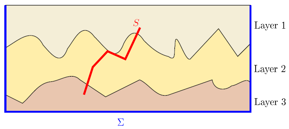
Figure 1. An example of the geometrical setting. A section of a layered medium with $S$, the dislocation surface, and with $\Sigma$, the buried part of $\Omega$.

Such boundary condition model the situation, where the relative motion of rock formations is small away from the fault as compared to that near the fault itself, except at the surface of the Earth due to the traction-free assumption there. A non-zero displacement on $\Sigma$ can also be imposed. Other types of boundary conditions on $\Sigma$ can be treated such as inhomogeneous Neumann boundary conditions, modeling the load bearing on the rock formations at the boundary from nearby formations. We assume the Earth’s crust to be a layered elastic medium, a common assumption in geophysics, that is, we assume that the elastic coefficients are piecewise regular, but may jump across a known partition of $\Omega$, see Figure 1, and impose standard transmission conditions at the interfaces of the partition. This set-up has been considered in the literature to model dislocations in geophysics (see for example [27, 28, 33]). The direct problem consists in solving a mixed-boundary-value-transmission problem for the elasticity system in $\Omega$, given in Equation (6).

In this work, we assume that the slip $\bm{g}$ vanishes at the boundary of the fault. This assumption is not overly restrictive in the geophysical context, where only patches of a fault are assumed active. The support of $\bm{g}$ can still be the entire fault surface, a situation that arises in the inverse problem. Then a variational solution exists for Problem (6), constructed by solving suitable auxiliary Neumann and mixed-boundary-value problems, after [1]. For the direct problem, well-posedness holds if the elasticity tensor $\mathbb{C}$ is an (anisotropic) bounded, strongly convex tensor.

For the inverse problem, we require more. On one hand, we need to guarantee that unique continuation for the elasticity system holds. This can be achieved by assuming that $\Omega$ is partitioned into finitely many Lipschitz subdomains and assuming that $\mathbb{C}$ is isotropic with Lamé coefficients Lipschitz continuous in each subdomain (see [3, 9, 10, 12] where a similar approach has been used to determine internal properties of an elastic medium from boundary measurements). On the other, the uniqueness proof, which uses an argument by contradiction, can be guaranteed to hold when $S$ is a graph with respect to an arbitrary, but chosen, coordinate system. This assumption is again not too restrictive in the geophysical context and allows for an arbitrary orientation of the surface (horizontal, vertical, or oblique). Differently than in [8], however, due the fact that the slip vanishes on the boundary of $S$, one does not need to assume $S$ has a corner singularity or assume a specific direction for the slip field $\bm{g}$. Therefore, the results presented here are a substantial generalization over known results for both the well-posedness of the direct and the uniqueness of the inverse problem.

The inverse dislocation problem has been treated both within the mathematics community [36], as well as in the geophysics community (among the extensive literature we mention [7, 25, 26] and references therein). Reconstruction has been tested primarily through iterative algorithms [36], based on Newton’s methods or constrained optimization of a suitable misfit functional, using either Boundary Integral methods or Finite Element methods, as well as Green’s function methods to solve the direct problem. For stochastic and statistical approaches to inversion we mention [20, 35] and references therein. We do not address here the question of reconstruction and its stability (see [11, 32]). This is focus of future work, which we plan to tackle by using appropriate iterative algorithms and solving the direct problem via Discontinuous Galerkin methods (for example adapting the methods in [5, 6]).

We close this Introduction with a brief outline of the paper. In Section 2, we introduce the relevant notation and the function spaces used throughout. In Section 3, we discuss the main assumptions on the coefficients and the geometry, and we address the well-posedness of the direct problem, while we discuss additional assumptions and prove uniqueness for the inverse problem in Section 4.

2. Notation and Functional Setting

We begin by introducing needed notation and the functional setting for both the direct as well as the inverse problem.

Notation: We denote scalar quantities in italics, e.g. $\lambda,\mu,\nu$, points and vectors in bold italics, e.g. $\bm{x},\bm{y},\bm{z}$ and $\bm{u},\bm{v},\bm{w}$, matrices and second-order tensors in bold face, e.g. $\mathbf{A},\mathbf{B},\mathbf{C}$, and fourth-order tensors in blackboard face, e.g. $\mathbb{A},\mathbb{B},\mathbb{C}$.

The symmetric part of a second-order tensor $\mathbf{A}$ is denoted by $\widehat{\mathbf{A}}=\tfrac{1}{2}\left(\mathbf{A}+\mathbf{A}^{T}\right)$, where $\mathbf{A}^{T}$ is the transpose matrix. In particular, $\widehat{\nabla\bm{u}}$ represents the deformation tensor. We utilize standard notation for inner products, that is, $\bm{u}\cdot\bm{v}=\sum_{i}u_{i}v_{i}$, and $\mathbf{A}:\mathbf{B}=\sum_{i,j}a_{ij}b_{ij}$. $|\mathbf{A}|$ denotes the norm induced by the inner product on matrices:

$$|\mathbf{A}|=\sqrt{\mathbf{A}:\mathbf{A}}.$$

Domains: Given $r>0$, we denote the ball of radius $r$ and center $\bm{x}$ by $B_{r}(\bm{x})\subset\mathbb{R}^{3}$ and a circle of radius $r$ and center $\bm{y}$ by $B^{\prime}_{r}(\bm{y})\subset\mathbb{R}^{2}$.

Definition 2.1 ($C^{k,\alpha}$ regularity of domains).

Let $\Omega$ be a bounded domain in $\mathbb{R}^{3}$. Given $k,\alpha$, with $k\in\mathbb{N}$ and $0<\alpha\leq 1$, we say that a portion $\Upsilon$ of $\partial\Omega$ is of class $C^{k,\alpha}$ with constant $r_{0}$, $E_{0}$, if for any $\bm{P}\in\Upsilon$, there exists a rigid transformation of coordinates under which we have $\bm{P}=\bm{0}$ and

$$\Omega\cap B_{r_{0}}(\bm{0})=\{\bm{x}\in B_{r_{0}}(\bm{0})\,:\,x_{3}>\psi(\bm{x}^{\prime})\},$$

where ${\psi}$ is a $C^{k,\alpha}$ function on $B^{\prime}_{r_{0}}(\bm{0})\subset\mathbb{R}^{2}$ such that

$${\psi}(\bm{0}) =0,$$

$$\nabla{\psi}(\bm{0}) =\mathbf{0},\qquad\text{for}\,k\geq 1$$

$$\|{\psi}\|_{C^{k,\alpha}(B^{\prime}_{r_{0}}(\bm{0}))} \leq E_{0}.$$

When $k=0,\alpha=1$, we also say that $\Upsilon$ is of Lipschitz class with constants $r_{0}$, $E_{0}$.

Given a bounded domain $\Omega\subset\mathbb{R}^{3}$ such that $\overline{\Omega}:=\overline{\Omega^{+}}\cup\overline{\Omega^{-}}$, where $\Omega^{+}$ and $\Omega^{-}$ are bounded domains, we call $f^{+}$ and $f^{-}$ the restriction of a function or distribution $f$ to ${\Omega^{+}}$ and $\Omega^{-}$, respectively. We denote the jump of a function or tensor field $\bm{f}$ across a bounded, oriented surface $S$ by $[\bm{f}]_{S}:=\bm{f}^{+}_{S}-\bm{f}^{-}_{S}$, where $\pm$ denotes a non-tangential limit to each side of the oriented surface $S$, $S^{+}$ and $S^{-}$, where $S^{+}$ is by convention the side where the unit normal vector $\bm{n}$ points into and $\bm{n}$ is determined by the given orientation on $S$.

Functional setting: we use standard notation to denote the usual functions spaces, e.g. $H^{s}(\Omega)$ denotes the $L^{2}$-based Sobolev space with regularity index $s\in\mathbb{R}$. $C^{\infty}_{0}(\Omega)$ is the space of smooth functions with compact support in $\Omega$.

We will need to consider trace spaces on open bounded surfaces that have a good extension property to closed surfaces containing them. (We refer to [19, 31] for an in-depth discussion). In what follows, $D$ is a given open bounded Lipschitz domain in $\mathbb{R}^{n}$, $n=2$ or $n=3$.

We recall that fractional Sobolev spaces on $D$ can be defined via real interpolation, and that $H^{s}_{0}(D):=\overline{C^{\infty}_{0}(D)}^{\|\cdot\|_{H^{s}(D)}}$, $s\geq 0$. We also recall that $H^{s}(D)=H^{s}_{0}(D)$, $0\leq s\leq 1/2$. If $s<1/2$, it is possible to extend an element of $H^{s}(D)$ by zero in $\mathbb{R}^{n}\setminus D$ to an element of $H^{s}(\mathbb{R}^{n})$. When $s=1/2$ such an extension is possible for elements that are suitably weighted by the distance to the boundary, since the extension operator from $H^{\frac{1}{2}}_{0}(D)$ to $H^{\frac{1}{2}}_{0}(\mathbb{R}^{n})$ is not continuous. Following Lions and Magenes [19], we introduce a smooth function, which is used to construct the weight, comparable to the distance to the boundary $d(x,\partial D)$.

Definition 2.2.

A function $\varrho$ such that $\varrho\in C^{\infty}(\overline{D})$, is positive in $D$, and vanishes on $\partial D$ with the same order as the distance to the boundary:

(1) $$\lim\limits_{x\to x_{0}}\frac{\varrho(x)}{d(x,\partial D)}=d\neq 0,\qquad\forall x_{0}\in\partial D,$$

is called a weight function.

Then we introduce the space $H^{\frac{1}{2}}_{00}(D)$ defined as

(2) $$H^{\frac{1}{2}}_{00}(D):=\Big{\{}u\in H^{\frac{1}{2}}_{0}(D),\varrho^{-1/2}u\in L^{2}(D)\Big{\}}.$$

This space is equipped with its natural norm, i.e.:

$$\|f\|_{H^{\frac{1}{2}}_{00}(D)}:=\|f\|_{H^{\frac{1}{2}}(D)}+\|\varrho^{-1/2}\,f\|_{L^{2}(D)},$$

which gives a finer topology than that in $H^{\frac{1}{2}}(D)$. If $v\in H^{\frac{1}{2}}_{00}(D)$, then its extension by zero to $\mathbb{R}^{n}\setminus D$ is an element of $H^{\frac{1}{2}}(\mathbb{R}^{n})$ and the extension operator is bounded. In particular, $v=0$ on $\partial D$ in trace sense. The space $H^{\frac{1}{2}}_{00}$ can also be identified with the real interpolation space

$$H^{\frac{1}{2}}_{00}(D)=(H^{1}_{0}(D),L^{2}(D))_{\frac{1}{2},2}.$$

Let $\mathcal{R}$ be the space of infinitesimal rigid motions in $\mathbb{R}^{3}$. To study the well-posedness of the direct problem, we introduce two variational spaces

(3) $$\mathring{H}^{1}(D)=\Bigg{\{}\bm{\eta}\in H^{1}(D):\,\,\,\int_{D}\bm{\eta}\cdot\bm{r}\,d\bm{x}=0,\forall\bm{r}\in\mathcal{R}\Bigg{\}},$$

and

(4) $${H}^{1}_{\Sigma}(D)=\Bigg{\{}\bm{\eta}\in H^{1}(D):\,\,\,\bm{\eta}|_{\Sigma}=\bm{0}\Bigg{\}},$$

where $\Sigma$ denotes the closure of an open subset of $\partial D$.

Finally, we denote the duality pairing between a Banach space $X$ and its dual $X^{\prime}$ with $\langle\cdot,\cdot\rangle_{(X^{\prime},X)}$. When clear from the context, we will omit the explicit dependence on the spaces, writing $\langle\cdot,\cdot\rangle$. We will write $\langle\cdot,\cdot\rangle_{D}$ to denote the pairing restricted to a domain $D$.

3. The direct problem

We first discuss the main assumptions on the dislocation surface $S$ and the elastic tensor $\mathbb{C}$, used in the rest of the paper. Then, we study the well-posedness of the forward problem.
Below $\Omega$ is a bounded Lipschitz domain.

Assumption 1 - elasticity tensor:

The elasticity tensor $\mathbb{C}=\mathbb{C}(\bm{x})$, a fourth-order totally symmetric tensor, is assumed uniformly bounded, $\mathbb{C}\in L^{\infty}(\Omega)$, and uniformly strongly convex, that is, $\mathbb{C}$ defines a positive-definite quadratic form on symmetric matrices:

$$\mathbb{C}(\bm{x})\widehat{\mathbf{A}}:\widehat{\mathbf{A}}\geq c|\widehat{\mathbf{A}}|,\qquad\textrm{a.e in}\,\,\Omega,$$

for $c>0$.

Assumption 2 - dislocation surface:

We model the dislocation surface $S$ by an open, bounded, oriented Lipschitz surface, with Lipschitz boundary, such that

(5) $$\overline{S}\subset\Omega.$$

We assume that $S$ can be extended to a closed Lipschitz, orientable surface $\Gamma$ satisfying

$$\Gamma\cap\partial\Omega=\emptyset.$$

Moreover, we indicate the domain enclosed by $\Gamma$ with $\Omega^{-}$ and $\Omega^{+}=\Omega\setminus\overline{\Omega^{-}}$. We choose the orientation on $S$ so that the associated normal $\bm{n}$ coincides with the unit outer normal to $\Omega^{-}$.

In this section, we study the following mixed-boundary-value problem:

(6) $$\begin{cases}\textrm{{div}}\,(\mathbb{C}\widehat{\nabla}\bm{u})=\bm{0},&\textrm{in}\,\,\Omega\setminus\overline{S},\\ (\mathbb{C}\widehat{\nabla}\bm{u})\bm{\nu}=\bm{0},&\textrm{on}\,\,\partial\Omega\setminus\Sigma,\\ \bm{u}=\bm{0},&\textrm{on}\,\,\Sigma\\ [\bm{u}]_{S}=\bm{g},\\ [(\mathbb{C}\widehat{\nabla}\bm{u})\bm{n}]_{S}=\bm{0},\\ \end{cases}$$

where $\Sigma$ is the closure of an open subset in $\partial\Omega$, $\bm{n}$ is the normal vector induced by the orientation on $S$ (see Assumption 2 - dislocation surface: ), $\bm{\nu}$ is the unit outer normal vector on $\partial\Omega$.

$\Omega$ represents a portion of the Earth’s crust where the fault $S$ lies and where both the direct and inverse problems are studied. $\Sigma$ models the buried part of the boundary of $\Omega$. Assuming that the rock displacement is zero on $\Sigma$ is justified from a geophysical point of view, as the relative motion of rock formations can be assumed much slower than rock slippage along an active fault. The complement of $\Sigma$ models the part of the boundary on the Earth’s crust and hence can be taken traction free. (See e.g. [33].)

The vector field $\bm{g}$ on $S$ models the slip along the active patch of the fault. We assume that

(7) $$\bm{g}\in H^{\frac{1}{2}}_{00}(S).$$

Recall that elements in this space have zero trace at the boundary, which is geophysically feasible as typically only parts of a fault are active.

Remark 3.1.

By hypothesis (see Assumption 2 - dislocation surface: ), $S$ is part of a closed Lipschitz surface $\Gamma$. Then, $\bm{g}\in H^{\frac{1}{2}}_{00}(S)$ implies that $\bm{g}$ can be extended by zero in $\Gamma\setminus S$ to a function $\widetilde{\bm{g}}\in H^{\frac{1}{2}}(\Gamma)$:

(8) $$\widetilde{\bm{g}}(\bm{x})=\begin{cases}\bm{g}(\bm{x}),&\textrm{if}\,\,\,\bm{x}\in S,\\ \bm{0},&\textrm{if}\,\,\,\bm{x}\in\Gamma\setminus S.\end{cases}$$

By a weak solution of (6) we mean that

(9) $$\begin{cases}\textrm{{div}}\,(\mathbb{C}\widehat{\nabla}\bm{u})=\bm{0},&\textrm{in}\,\,\left(H^{1}_{\Sigma}(\Omega)\right)^{\prime}\\ (\mathbb{C}\widehat{\nabla}\bm{u})\bm{\nu}=\bm{0},&\textrm{in}\,\,H^{-\frac{1}{2}}(\partial\Omega\setminus\Sigma),\\ \bm{u}=\bm{0},&\textrm{in}\,\,H^{\frac{1}{2}}(\Sigma)\\ [\bm{u}]_{S}=\bm{g},&\textrm{in}\,\,H^{\frac{1}{2}}_{00}(S)\\ [(\mathbb{C}\widehat{\nabla}\bm{u})\bm{n}]_{S}=\bm{0},&\textrm{in}\,\,H^{-\frac{1}{2}}(S)\\ \end{cases}$$

The strategy that we follow here is an adaptation of the procedure described in [2] to solve classical transmission problems. Given the closed surface $\Gamma$ and the extension (8), we decompose $\Omega$ into two domains $\Omega^{-}$ and $\Omega^{+}$, as in Assumption 2 - dislocation surface: . Then we construct a weak solution of Problem (6) by solving two boundary-value problems, one in $\Omega^{-}$ and one $\Omega^{+}$, imposing suitable Neumann conditions on $\Gamma$. The key step in this procedure consists in identifying the proper Neumann boundary condition on $\Gamma$ such that $[\bm{u}]_{\Gamma}=\bm{u}^{+}_{\Gamma}-\bm{u}^{-}_{\Gamma}=\widetilde{\bm{g}}$, where $\bm{u}^{+}_{\Gamma}$ and $\bm{u}^{-}_{\Gamma}$ are the traces on $\Gamma$ of the solutions $\bm{u}^{+}$ in $\Omega^{+}$ and $\bm{u}^{-}$ in $\Omega^{-}$, respectively. In $\Omega^{-}$, the solution $\bm{u}^{-}$ will be sought in the auxiliary space $\mathring{H}^{1}(\Omega^{-})$ to ensure uniqueness. This choice imposes apparently artificial normalization conditions in $\Omega^{-}$, which are not needed to solve the original problem (6). However, we can verify a posteriori that such conditions are in fact satisfied by the unique solution to the original problem.

We shall first prove some preliminary results.

Lemma 3.2.

Let $\overline{\Omega}=\overline{\Omega^{+}}\cup\overline{\Omega^{-}}$, where $\Omega^{+}$ and $\Omega^{-}$ are defined in Assumption 2 - dislocation surface: . Let

(10) $$\widetilde{H}:=\Big{\{}f\in L^{2}(\Omega):\,\,f^{+}\in H^{1}(\Omega^{+}),\,f^{-}\in H^{1}(\Omega^{-}),\textup{{and}}\,\,[f]_{\Gamma\setminus\overline{S}}=0\Big{\}},$$

where $f^{+}=f\lfloor_{\Omega^{+}}$ and $f^{-}=f\lfloor_{\Omega^{-}}$. Then

$$H^{1}(\Omega\setminus\overline{S})\cong\widetilde{H}.$$

This result is classical (see e.g. [1] for a proof using Green’s formula in Lipschitz domains, obtained in [21]). We include here the proof for the reader’s sake.

Proof.

Let $f\in\widetilde{H}$ and let $\bm{\varphi}\in C^{\infty}(\overline{\Omega})$ with support in $\Omega\setminus\overline{S}$. We apply the Divergence Theorem in $\Omega^{+}$ and $\Omega^{-}$, obtaining

$$\int_{\Omega^{-}}\nabla f^{-}\cdot\bm{\varphi}\,d\bm{x}=\int_{\Gamma}f^{-}\bm{n}\cdot\bm{\varphi}^{-}\,d\sigma(\bm{x})-\int_{\Omega^{-}}f^{-}\,\textrm{div}\,\bm{\varphi}\,d\bm{x},$$

where $\bm{n}$ is the unit outer normal vector to $\Omega^{-}$. Similarly

$$\int_{\Omega^{+}}\nabla f^{+}\cdot\bm{\varphi}\,d\bm{x}=-\int_{\Gamma}f^{+}\bm{n}\cdot\bm{\varphi}^{+}\,d\sigma(\bm{x})-\int_{\Omega^{+}}f^{+}\,\textrm{div}\,\bm{\varphi}\,d\bm{x}.$$

Therefore, we find

$$\int_{\Omega^{-}}\nabla f^{-}\cdot\bm{\varphi}\,d\bm{x}+\int_{\Omega^{+}}\nabla f^{+}\cdot\bm{\varphi}\,d\bm{x}=\int_{\Gamma\setminus\overline{S}}\left(f^{-}\bm{\varphi}^{-}-f^{+}\bm{\varphi}^{+}\right)\cdot\bm{n}\,d\sigma(\bm{x})-\int_{\Omega\setminus\overline{S}}f\,\textrm{div}\,\bm{\varphi}\,d\bm{x},$$

noting in the terms on the right that $\bm{\varphi}$ and $\textrm{div}\,\bm{\varphi}$ have compact support in $\Omega\setminus\overline{S}$ and, as an $L^{2}$ function, $f=f^{+}\chi_{\Omega^{+}}+f^{-}\chi_{\Omega^{-}}$. Moreover, $\bm{\varphi}$ is regular across $\Gamma\setminus\overline{S}$ by hypothesis and $f^{+}=f^{-}$ on $\Gamma\setminus\overline{S}$, since $f\in\widetilde{H}$, so that

$$\int_{\Gamma\setminus\overline{S}}\left(f^{-}\bm{\varphi}^{-}-f^{+}\bm{\varphi}^{+}\right)\cdot\bm{n}\,d\sigma(\bm{x})=\int_{\Gamma\setminus\overline{S}}\bm{\varphi}\,\left(f^{-}-f^{+}\right)\cdot\bm{n}\,d\sigma(\bm{x})=0.$$

Consequently,

$$\int_{\Omega\setminus\overline{S}}f\,\textrm{div}\,\bm{\varphi}\,d\bm{x}=-\int_{\Omega^{+}}\nabla f^{+}\cdot\bm{\varphi}\,d\bm{x}-\int_{\Omega^{-}}\nabla f^{-}\cdot\bm{\varphi}\,d\bm{x},$$

which means that the distributional gradient of $f$ is an $L^{2}$ function in $\Omega\setminus\overline{S}$ and agrees with

$$\nabla f^{+}\chi_{\Omega^{+}}+\nabla f^{-}\chi_{\Omega^{-}}.$$

Reversing the argument gives the opposite implication. ∎

For the next lemma, we follow [2, Proposition 12.8.2], adapting that result to the case of the Lamé operator with discontinuous coefficients.

Lemma 3.3.

Let $\mathbb{C}\in L^{\infty}(\Omega)$, and let $\bm{\eta}\in{H}^{1}(\Omega\setminus\overline{S})$ be a weak solution of the system $\textrm{div}(\mathbb{C}\widehat{\nabla}\bm{\eta})=\bm{0}$ in $\Omega\setminus\overline{S}$. Then $[(\mathbb{C}\widehat{\nabla}\bm{\eta})\bm{n}]_{\Gamma\setminus\overline{S}}=\bm{0}$ in $H^{-\frac{1}{2}}(\Gamma\setminus\overline{S})$.

Proof.

We fix a point $\bm{x}_{0}\in\Gamma\setminus\overline{S}$ and we consider a ball $B_{r}(\bm{x}_{0})$ with $r>0$ sufficiently small so that $B_{r}(\bm{x}_{0})\cap\overline{S}=\emptyset$ and $B_{r}(\bm{x}_{0})\cap\partial\Omega=\emptyset$.
Let $\bm{\varphi}\in H^{1}_{0}(B_{r}(\bm{x}_{0}))$, then

(11) $$0=\langle\textrm{div}(\mathbb{C}\widehat{\nabla}\bm{\eta}),\bm{\varphi}\rangle=-\int_{B_{r}(\bm{x}_{0})}\mathbb{C}\widehat{\nabla}\bm{\eta}:\widehat{\nabla}\bm{\varphi}\,d\bm{x}.$$

(This identity can be established by approximating $\bm{\varphi}$ with smooth fields supported in $B_{r}(\bm{x}_{0})$.)

Next we apply Green’s identities, which hold for $H^{1}$-functions, in $D^{+}=B_{r}(\bm{x}_{0})\cap\Omega^{+}$ and $D^{-}=B_{r}(\bm{x}_{0})\cap\Omega^{-}$. Therefore, for all $\bm{\varphi}\in H^{1}_{0}(B_{r}(\bm{x}_{0}))$,

(12) $$0=-\int_{D^{+}}\mathbb{C}\widehat{\nabla}\bm{\eta}:\widehat{\nabla}\bm{\varphi}\,d\bm{x}-\langle\mathbb{C}\widehat{\nabla}\bm{\eta}^{+}\bm{n},\bm{\varphi}^{+}\rangle_{(H^{-\frac{1}{2}}(\Gamma\cap\partial D^{+}),H^{\frac{1}{2}}(\Gamma\cap\partial D^{+}))}$$

and, analogously,

(13) $$0=-\int_{D^{-}}\mathbb{C}\widehat{\nabla}\bm{\eta}:\widehat{\nabla}\bm{\varphi}\,d\bm{x}+\langle\mathbb{C}\widehat{\nabla}\bm{\eta}^{-}\bm{n},\bm{\varphi}^{-}\rangle_{(H^{-\frac{1}{2}}(\Gamma\cap\partial D^{-}),H^{\frac{1}{2}}(\Gamma\cap\partial D^{-}))}.$$

Since $\bm{\varphi}\in H^{1}_{0}(B_{r}(\bm{x}_{0}))$, $\bm{\varphi}^{+}_{|_{\Gamma\cap B_{r}(\bm{x}_{0})}}=\bm{\varphi}^{-}_{|_{\Gamma\cap B_{r}(\bm{x}_{0})}}=:\bm{\varphi}_{|_{\Gamma\cap B_{r}(\bm{x}_{0})}}$. Hence, adding (12) and (13) gives:

$$0=-\int_{D^{+}}\mathbb{C}\widehat{\nabla}\bm{\eta}:\widehat{\nabla}\bm{\varphi}\,d\bm{x}-\int_{D^{-}}\mathbb{C}\widehat{\nabla}\bm{\eta}:\widehat{\nabla}\bm{\varphi}\,d\bm{x}-\langle[\mathbb{C}\widehat{\nabla}\bm{\eta}\bm{n}],\bm{\varphi}\rangle_{(H^{-\frac{1}{2}}(\Gamma\cap B_{r}(\bm{x}_{0})),H^{\frac{1}{2}}(\Gamma\cap B_{r}(\bm{x}_{0})))},$$

where $[,]$ denotes the jump across $\Gamma\cap B_{r}(\bm{x}_{0})$. Consequently,

$$0=-\int_{B_{r}(\bm{x}_{0})}\mathbb{C}\widehat{\nabla}\bm{\eta}:\widehat{\nabla}\bm{\varphi}\,d\bm{x}-\langle[\mathbb{C}\widehat{\nabla}\bm{\eta}\bm{n}],\bm{\varphi}\rangle_{(H^{-\frac{1}{2}}(\Gamma\cap B_{r}(\bm{x}_{0})),H^{\frac{1}{2}}(\Gamma\cap B_{r}(\bm{x}_{0})))},$$

using that, by hypothesis, both $\nabla\bm{\varphi}$ and $\nabla\bm{\eta}$ exists as $L^{2}$ functions in $B_{r}(\bm{r}_{0})$. From (11) it follows that

$$\langle[\mathbb{C}\widehat{\nabla}\bm{\eta}\bm{n}],\bm{\varphi}\rangle_{(H^{-\frac{1}{2}}(\Gamma\cap B_{r}(\bm{x}_{0})),H^{\frac{1}{2}}(\Gamma\cap B_{r}(\bm{x}_{0})))}=0.$$

Since $\bm{\varphi}$ is an arbitrary function in $H^{1}_{0}(B_{r}(\bm{x}_{0}))$, we have that $[\mathbb{C}\widehat{\nabla}\bm{\eta}\bm{n}]_{{\Gamma\cap B_{r}(\bm{x}_{0})}}=\bm{0}$ in $H^{-\frac{1}{2}}(\Gamma\setminus\overline{S})$. We conclude by covering $\Gamma\setminus\overline{S}$ with a finite number of balls $B_{r}(\bm{x}_{i})$, $i=1,\ldots,N$. ∎

We are now ready to tackle the well-posedness of Problem (6). We begin by addressing the uniqueness of weak solutions.

Theorem 3.4.

(Uniqueness) Problem (6) has at most one weak solution in ${H}^{1}_{\Sigma}(\Omega\setminus\overline{S})$.

Proof.

Assume that there exist two solutions $\bm{u}^{1},\bm{u}^{2}\in{H}^{1}_{\Sigma}(\Omega\setminus\overline{S})$. Let $\bm{v}=\bm{u}^{1}-\bm{u}^{2}$. From the transmission conditions on $S$ (see (6)), we have

$$[\bm{v}]_{S}=\bm{0},\qquad\qquad[(\mathbb{C}\widehat{\nabla}\bm{v})\bm{n}]_{S}=\bm{0}.$$

Hence, by Lemma 3.2, $\bm{v}\in{H}^{1}_{\Sigma}(\Omega)$. It follows that $\bm{v}$ is a weak solution of the problem

(14) $$\begin{cases}\textrm{div}(\mathbb{C}\widehat{\nabla}\bm{v})=\bm{0}\,&\text{in}\,\,\Omega\\ (\mathbb{C}\widehat{\nabla}\bm{v})\bm{\nu}=\bm{0}&\textrm{on}\,\,\partial\Omega\setminus\Sigma\\ \bm{v}=\bm{0}&\textrm{on}\,\,\Sigma,\end{cases}$$

which has a unique solution, $\bm{v}=\bm{0}$.

∎

Theorem 3.5.

(Existence) There exists a weak solution $\bm{u}\in{H}^{1}_{\Sigma}(\Omega\setminus\overline{S})$ to Problem (6).

Proof.

We consider the following Neumann boundary-value problem in $\mathring{H}^{1}(\Omega^{-})$ (the space is chosen in order to avoid rigid motions in $\Omega^{-}$):

(15) $$\begin{cases}\textrm{div}(\mathbb{C}\widehat{\nabla}\bm{u}^{-})=\bm{0},&\textrm{in}\,\,\,\Omega^{-}\\ (\mathbb{C}\widehat{\nabla}\bm{u}^{-})\bm{n}=\bm{\varphi},&\textrm{on}\,\,\,\Gamma\end{cases}$$

and the following mixed-boundary-value problem in ${H}^{1}_{\Sigma}(\Omega^{+})$:

(16) $$\begin{cases}\textrm{div}(\mathbb{C}\widehat{\nabla}\bm{u}^{+})=\bm{0},&\textrm{in}\,\,\,\Omega^{+}\\ (\mathbb{C}\widehat{\nabla}\bm{u}^{+})\bm{\nu}=\bm{0},&\textrm{on}\,\,\,\partial\Omega\setminus\Sigma\\ \bm{u}^{+}=\bm{0},&\textrm{on}\,\,\,\Sigma\\ (\mathbb{C}\widehat{\nabla}\bm{u}^{+})\bm{n}=\bm{\varphi},&\textrm{on}\,\,\,\Gamma,\end{cases}$$

where $\Omega^{-}$ and $\Omega^{+}$ are defined in Assumption 2 - dislocation surface: .
The key point of the proof is to identify $\bm{\varphi}$ in order to represent the solution $\bm{u}$ of (6) as $\bm{u}=\bm{u}^{-}\chi_{\Omega^{-}}+\bm{u}^{+}\chi_{\Omega^{+}}$, where $\chi_{\Omega^{-}}$ and $\chi_{\Omega^{+}}$ are the characteristic functions of the sets $\Omega^{-}$ and $\Omega^{+}$, respectively. To this end, we define the bounded Neumann-Dirichlet operators

$$N^{+}:H^{-\frac{1}{2}}(\Gamma)\to H^{\frac{1}{2}}(\Gamma),\qquad\qquad N^{-}:H^{-\frac{1}{2}}(\Gamma)\to H^{\frac{1}{2}}(\Gamma),$$

where $N^{+}$ and $N^{-}$ are such that $N^{+}\bm{\varphi}=\widetilde{\bm{g}}^{+}$ and $N^{-}\bm{\varphi}=\widetilde{\bm{g}}^{-}$, where $\widetilde{\bm{g}}^{+}:=\bm{u}^{+}_{\Gamma}$ and $\widetilde{\bm{g}}^{-}:=\bm{u}^{-}_{\Gamma}$, the traces of $\bm{u}^{+}$ and $\bm{u}^{-}$ on $\Gamma$. Therefore, we need to identify $\bm{\varphi}\in H^{-\frac{1}{2}}(\Gamma)$ such that

(17) $$(N^{+}-N^{-})\bm{\varphi}=\widetilde{\bm{g}},$$

where $\widetilde{\bm{g}}$ is the extension of $\bm{g}$ on $\Gamma\setminus S$, as defined in (8).
The invertibility of the operator $N^{+}-N^{-}$ guarantees that $\bm{\varphi}=(N^{+}-N^{-})^{-1}(\widetilde{\bm{g}})$, and follows from the continuity of both the Neumann-to-Dirichlet and the Dirichlet-to-Neumann maps. Such continuity is well known. We briefly outline here a proof of invertibility in our setting for the reader’s sake.

First, by using the weak formulation of (15) in $\mathring{H}^{1}(\Omega^{-})$ and (16) in ${H}^{1}_{\Sigma}(\Omega^{+})$, we find a relation between the quadratic form associated to (15) and $\langle\bm{\varphi},N^{-}\bm{\varphi}\rangle_{\Gamma}$, and between the quadratic form associated to (16) and $\langle\bm{\varphi},N^{+}\bm{\varphi}\rangle_{\Gamma}$. Indeed, from the weak formulation of problems (15) and (16), we find that

(18) $$\int_{\Omega^{+}}\mathbb{C}\widehat{\nabla}\bm{u}^{+}\cdot\widehat{\nabla}\bm{v}^{+}\,d\bm{x}=-\langle\bm{\varphi},\bm{v}^{+}\rangle_{\Gamma},\qquad\qquad\forall\bm{v}^{+}\in{H}^{1}_{\Sigma}(\Omega^{+}),$$

as $\bm{n}$ points inwards in $\Omega^{+}$, and that

(19) $$\int_{\Omega^{-}}\mathbb{C}\widehat{\nabla}\bm{u}^{-}\cdot\widehat{\nabla}\bm{v}^{-}\,d\bm{x}=\langle\bm{\varphi},\bm{v}^{-}\rangle_{\Gamma},\qquad\qquad\forall\bm{v}^{-}\in H^{1}(\Omega^{-}).$$

Next, we observe that we can extend any function $\bm{v}\in H^{\frac{1}{2}}(\Gamma)$ to, respectively, functions $\bm{v}^{+}\in H^{1}_{\Sigma}(\Omega^{+})$ and $\bm{v}^{-}\in H^{1}(\Omega^{-})$, for instance by solving suitable Dirichlet problems for the Laplace operator in $\Omega^{+}$ and $\Omega^{-}$. Then, the above identities imply:

$$|\langle\bm{\varphi},\bm{v}\rangle_{\Gamma}|\leq C_{\pm}\,\|\bm{u}^{\pm}\|_{H^{1}(\Omega^{\pm})}\,\|\bm{v}^{\pm}\|_{H^{1}(\Omega^{\pm})}\leq C_{\pm}\,\|\bm{u}^{\pm}\|_{H^{1}(\Omega^{\pm})}\,\|\bm{v}\|_{H^{\frac{1}{2}}(\Gamma)}.$$

Using the definition of the norm in $H^{-\frac{1}{2}}(\Gamma)$ as the operator norm of functionals on $H^{\frac{1}{2}}(\Gamma)$, it follows that

(20) $$\|\bm{\varphi}\|_{H^{-\frac{1}{2}}(\Gamma)}\leq C_{\pm}\|\bm{u}^{\pm}\|_{H^{1}(\Omega^{\pm})}.$$

Moreover, by choosing $\bm{v}^{+}=\bm{u}^{+}$ in (18) and $\bm{v}^{-}=\bm{u}^{-}$ in (19), we have:

$$\int_{\Omega^{+}}\mathbb{C}\widehat{\nabla}\bm{u}^{+}\cdot\widehat{\nabla}\bm{u}^{+}\,d\bm{x}=-\langle\bm{\varphi},N^{+}\bm{\varphi}\rangle_{\Gamma},$$

and

$$\int_{\Omega^{-}}\mathbb{C}\widehat{\nabla}\bm{u}^{-}\cdot\widehat{\nabla}\bm{u}^{-}\,d\bm{x}=\langle\bm{\varphi},N^{-}\bm{\varphi}\rangle_{\Gamma}.$$

Then Assumption 1 - elasticity tensor: , Korn’s and Poincaré’s inequalities (see e.g. [24]) give that

(21) $$-\langle\bm{\varphi},N^{+}\bm{\varphi}\rangle_{\Gamma}=\int_{\Omega^{+}}\mathbb{C}\widehat{\nabla}\bm{u}^{+}\cdot\widehat{\nabla}\bm{u}^{+}\,d\bm{x}\geq C\|\bm{u}^{+}\|^{2}_{{H}^{1}(\Omega^{+})},$$

and that

(22) $$\langle\bm{\varphi},N^{-}\bm{\varphi}\rangle_{\Gamma}=\int_{\Omega^{-}}\mathbb{C}\widehat{\nabla}\bm{u}^{-}\cdot\widehat{\nabla}\bm{u}^{-}\,d\bm{x}\geq C\|\bm{u}^{-}\|^{2}_{\mathring{H}^{1}(\Omega^{-})}.$$

Therefore, by using (20) in both (21) and (22), we can establish the coercivity of the bilinear form associated to Equation (17), that is,

(23) $$\|\bm{\varphi}\|^{2}_{H^{-\frac{1}{2}}(\Gamma)}\leq C\langle\bm{\varphi},(-N^{+}+N^{-})\bm{\varphi}\rangle_{\Gamma}.$$

The continuity of this form follows directly from the continuity of the solution operators for (15)-(16) and the Trace Theorem. The Lax-Milgram Theorem then ensures that there exists a unique solution $\bm{\varphi}\in H^{-\frac{1}{2}}(\Gamma)$ such that

(24) $$\langle\bm{\psi},(-N^{+}+N^{-})\bm{\varphi}\rangle_{\Gamma}=\langle\bm{\psi},-\widetilde{\bm{g}}\rangle_{\Gamma},\qquad\forall\bm{\psi}\in H^{-\frac{1}{2}}(\Gamma),$$

namely the operator $-N^{+}+N^{-}$ is invertible.

With this choice of $\bm{\varphi}$, Problems (15) and (16) admit unique solutions $\bm{u}^{-}\in\mathring{H}^{1}(\Omega^{-})$ and $\bm{u}^{+}\in{H}^{1}_{\Sigma}(\Omega^{+})$, respectively. Next, we let

$$\bm{u}=\bm{u}^{-}\chi_{\Omega^{-}}+\bm{u}^{+}\chi_{\Omega^{+}}.$$

Then, $\bm{u}=\bm{u}^{-}\in H^{1}(\Omega^{-})$, $\bm{u}=\bm{u}^{+}\in H^{1}(\Omega^{+})$, $\bm{u}$ is a distributional solution of $\text{div}(\mathbb{C}\widehat{\nabla}\bm{u})=\bm{0}$ in $\Omega^{+}$ and $\Omega^{-}$. To conclude, we show that $\bm{u}$ is a weak solution of (6). By construction, it follows that $\bm{u}$ satisfies the boundary conditions on $\partial\Omega$ in trace sense. Again by construction

$$[\bm{u}]_{\Gamma}=\bm{u}^{+}_{\Gamma}-\bm{u}^{-}_{\Gamma}=\widetilde{\bm{g}}\quad\text{in }H^{\frac{1}{2}}(\Gamma).$$

That is, by (8),

(25) $$[\bm{u}]_{\Gamma\setminus\overline{S}}=\bm{0},\qquad\qquad[\bm{u}]_{{S}}=\bm{g},$$

hence, by Lemma 3.2, it follows that $\bm{u}\in H^{1}(\Omega\setminus\overline{S})$. Moreover,

(26) $$[\mathbb{C}\widehat{\nabla}\bm{u}\,\bm{n}]_{\Gamma}=\bm{0}\quad\text{in }H^{-\frac{1}{2}}(\Gamma),$$

which follows immediately by construction. In particular, $[\mathbb{C}\widehat{\nabla}\bm{u}\,\bm{n}]_{S}=\bm{0}$. Now, recalling that $\bm{u}$ is a weak solution in $\Omega^{-}$ and in $\Omega^{+}$ and satisfies (26), reversing the steps in the proof of Lemma 3.3, we obtain that $\bm{u}$ is a weak solution of $\textrm{div}(\mathbb{C}\widehat{\nabla}\bm{u})=\bm{0}$ in $\Omega\setminus\overline{S}$. ∎

We note that, from the proof of the existence theorem above, a weak solution is also a variational solution in the following sense: $\bm{u}\in H^{1}_{\Sigma}(\Omega^{+})$, $\bm{u}\in{H}^{1}(\Omega^{-})$, $[\bm{u}]_{\Gamma}=\widetilde{\bm{g}}$ in $H^{\frac{1}{2}}(\Gamma)$ and $\bm{u}$ is such that, for every $\bm{v}\in H^{1}_{\Sigma}(\Omega)$,

(27) $$\int_{\Omega^{+}}\mathbb{C}\widehat{\nabla}\bm{u}\cdot\widehat{\nabla}\bm{v}\,d\bm{x}+\int_{\Omega^{-}}\mathbb{C}\widehat{\nabla}\bm{u}\cdot\widehat{\nabla}\bm{v}\,d\bm{x}=0.$$

We observe that a variational solution could also be obtained by a suitable lift, see for example [17].

Corollary 3.6.

There exists a unique solution $\bm{u}\in H^{1}_{\Sigma}(\Omega\setminus\overline{S})$ to Problem (6).

We observe that other types of boundary conditions can, in principle, be imposed on the buried part $\Sigma$ of $\partial\Omega$. For example, one can impose a non-homogeneous traction there, modeling the load of contiguous rock formations on $\Omega$ itself.

Remark 3.7.

The approach to proving well-posedness for (6) can be adapted to other boundary value problems as well, such as Neumann problems with non-homogeneous boundary conditions on $\partial\Omega$. In fact, given $\bm{h}\in H^{-\frac{1}{2}}(\partial\Omega)$, one can show that there exists a unique solution $\bm{u}_{N}\in\mathring{H}^{1}(\Omega\setminus\overline{S})$ for the following problem:

(28) $$\begin{cases}\textrm{{div}}\,(\mathbb{C}\widehat{\nabla}\bm{u}_{N})=\bm{0},&\textrm{in}\,\,\Omega\setminus\overline{S},\\ (\mathbb{C}\widehat{\nabla}\bm{u}_{N})\bm{\nu}=\bm{h},&\textrm{on}\,\,\partial\Omega,\\ [\bm{u}_{N}]_{S}=\bm{g},\\ [(\mathbb{C}\widehat{\nabla}\bm{u}_{N})\bm{n}]_{S}=\bm{0},\\ \end{cases}$$

The proof of uniqueness in $\mathring{H}^{1}(\Omega\setminus\overline{S})$ follows exactly as in Theorem 3.4. For the proof of existence, we notice that due to the linearity property of (28), $\bm{u}_{N}$ can be decomposed as $\bm{u}_{N}:=\mathring{\bm{u}}+\bm{w}$, where $\mathring{\bm{u}}\in\mathring{H}^{1}(\Omega\setminus\overline{S})$ is the unique solution to

(29) $$\begin{cases}\textrm{{div}}\,(\mathbb{C}\widehat{\nabla}\mathring{\bm{u}})=\bm{0},&\textrm{in}\,\,\Omega\setminus\overline{S},\\ (\mathbb{C}\widehat{\nabla}\mathring{\bm{u}})\bm{\nu}=\bm{0},&\textrm{on}\,\,\partial\Omega,\\ [\mathring{\bm{u}}]_{S}=\bm{g},\\ [(\mathbb{C}\widehat{\nabla}\mathring{\bm{u}})\bm{n}]_{S}=\bm{0},\\ \end{cases}$$

and $\bm{w}\in\mathring{H}^{1}(\Omega)$ is solution to

(30) $$\begin{cases}\textrm{{div}}\,(\mathbb{C}\widehat{\nabla}\bm{w})=\bm{0},&\textrm{in}\,\,\Omega\setminus\overline{S},\\ (\mathbb{C}\widehat{\nabla}\bm{w})\bm{\nu}=\bm{h},&\textrm{on}\,\,\partial\Omega,\\ [\bm{w}]_{S}=\bm{0},\\ [(\mathbb{C}\widehat{\nabla}\bm{w})\bm{n}]_{S}=\bm{0}.\end{cases}$$

The proof of existence of a solution $\mathring{\bm{u}}\in\mathring{H}^{1}(\Omega\setminus\overline{S})$ for (29) then follows the same ideas as in Theorem 3.5, but with the simplification that both $\bm{u}^{+}$ and $\bm{u}^{-}$ belong now to the same space $\mathring{H}^{1}$. Problem (30) is reduced to a standard transmission problem, hence the existence of a unique solution in $\mathring{H}^{1}(\Omega)$ follows easily.

4. The Inverse Problem: a uniqueness result

In this section we address the uniqueness for the inverse dislocation problem, which consists in identifying the dislocation $S$ and the slip $\bm{g}$ on it from displacement measurements made at the surface of the Earth. Uniqueness will be proved under additional assumptions on the geometry and the data for Problem (6). In particular, we consider a domain $\Omega$ which is partitioned in finitely-many Lipschitz subdomains, we assume that the elasticity tensor is isotropic with Lamé coefficients Lipschitz continuous in each subdomain, and we take the dislocation surface to be a graph with respect to a fixed, but arbitrary, coordinate frame. Such assumptions are not unrealistic in the context of geophysical applications and underscores the ill-posedness of the inverse problems without additional a priori information.

Specifically, in additions to Assumption 1 - elasticity tensor: and Assumption 2 - dislocation surface: , we assume the following:

Assumption 3 - domain and partition:

We denote by $\Xi\subseteq(\partial\Omega\setminus\overline{\Sigma})$ an open patch of the boundary where the measurements of the displacement field are given. Moreover, we assume that

$$\overline{\Omega}=\bigcup\limits_{k=1}^{N}\overline{D_{k}}$$

where $D_{k}$, for $k=1,\cdots N$, are pairwise non-overlapping bounded Lipschitz domains. We assume, without loss of generality, that $\Xi$ is contained in $\partial D_{1}$.

Assumption 4 - elasticity tensor:

The elasticity tensor $\mathbb{C}=\mathbb{C}(\bm{x})$ is assumed isotropic in each element of the partition of $\Omega$, i.e.,

(31) $$\mathbb{C}(\bm{x})=\sum_{k=1}^{N}\mathbb{C}_{k}(\bm{x})\chi_{D_{k}}(\bm{x}),\qquad\mathbb{C}_{k}(\bm{x}):=\lambda_{k}(\bm{x})\mathbf{I}\otimes\mathbf{I}+2\mu_{k}(\bm{x})\mathbb{I},$$

where $\lambda_{k}=\lambda_{k}(\bm{x})$ and $\mu_{k}=\mu_{k}(\bm{x})$, for $k=1,\cdots,N$, are the Lamé coefficients related to the subdomain $D_{k}$, $\mathbf{I}$ and $\mathbb{I}$ the identity matrix and the identity fourth-order tensor, respectively. Each Lamé parameter, $\lambda_{k},\mu_{k}$, for $k=1,\cdots,N$, belongs to $C^{0,1}(\overline{D_{k}})$, that is, there exists $M>0$ such that

(32) $$\|\mu_{k}\|_{C^{0,1}(\overline{D_{k}})}+\|\lambda_{k}\|_{C^{0,1}(\overline{D_{k}})}\leq M,$$

with $\|\cdot\|_{C^{0,1}(\overline{D_{k}})}=\|\cdot\|_{L^{\infty}(\overline{D_{k}})}+\|\nabla\cdot\|_{L^{\infty}(\overline{D_{k}})}$. Finally, there exist two positive constants $\alpha_{0},\beta_{0}$ such that,

(33) $$\mu_{k}(\bm{x})\geq\alpha_{0}>0,\quad 3\lambda_{k}(\bm{x})+2\mu_{k}(\bm{x})\geq\beta_{0}>0,\qquad\forall\bm{x}\in\overline{D_{k}},\quad k=1,\ldots,N.$$

These conditions ensures the uniform strong convexity of $\Omega$.

Our main result for the inverse problem is the following theorem.

Theorem 4.1.

Under Assumption 3 - domain and partition: and Assumption 4 - elasticity tensor: , let $S_{1},S_{2}$ be as in Assumption 2 - dislocation surface: and such that ${S}_{1},{S}_{2}$, are graphs with respect to a fixed but arbitrary coordinate frame. Let $\bm{g}_{i}\in H^{\frac{1}{2}}_{00}(S_{i})$, for $i=1,2$, with Supp$\,\bm{g}_{i}=\overline{S}_{i}$, for $i=1,2$, and $\bm{u}_{i}$, for $i=1,2$, be the unique solution of (6) in $H^{1}_{\Sigma}(\Omega\setminus\overline{S})$ corresponding to $\bm{g}=\bm{g}_{i}$ and $S=S_{i}$. If $\bm{u}_{1\big{|}_{\Xi}}=\bm{u}_{2\big{|}_{\Xi}}$, then $S_{1}=S_{2}$ and $\bm{g}_{1}=\bm{g}_{2}$.

We denote by $G$ the connected component of $\Omega\setminus\overline{S_{1}\cup S_{2}}$ containing $\Xi$. By definition we have that $G\subseteq(\Omega\setminus\overline{S_{1}\cup S_{2}})$. In addition, we define

(34) $$\mathcal{G}:=\partial G\setminus\partial\Omega.$$

Before proving Theorem 4.1, we recall the following lemma proved in [8] in the special case where $\Omega$ is a half-space. However, this result is clearly true for bounded domains as well.

Lemma 4.2.

Let $S_{1},S_{2}$ as in Assumption 2 - dislocation surface: and such that ${S}_{1},{S}_{2}$, are graphs with respect to a fixed but arbitrary coordinate frame. Then $\mathcal{G}=\overline{S_{1}\cup S_{2}}$.

Proof of Theorem 4.1.

We first show that $\bm{w}:=\bm{u}_{1}-\bm{u}_{2}$ is identically zero in $G$. We can assume, without loss of generality, that $\Xi$ is the graph of a Lipschitz function in some coordinate frame, say with respect to the $z$-axis. In fact, it is enough to take a possibly small open subset of $\Xi$ instead of the entire $\Xi$, and then this hypothesis is always satisfied as $\partial\Omega$ is assumed globally Lipschitz. On $\Xi$ we have that

$$\bm{w}=\bm{0},\qquad(\mathbb{C}\widehat{\nabla}\bm{w})\bm{\nu}=\bm{0},$$

Then, fixing a point $\bm{x}_{0}\in\Xi$, we consider $B_{R}(\bm{x}_{0})$, the ball of radius $R$ and center $\bm{x}_{0}$, where $R$ is taken sufficiently small so that $B_{R}(\bm{x}_{0})\cap\Xi\subseteq\Xi$ and we denote by $B^{-}_{R}(\bm{x}_{0}):=B_{R}(\bm{x}_{0})\cap\overline{\Omega}$ and $B^{+}_{R}(\bm{x}_{0})=(B^{-}_{R}(\bm{x}_{0}))^{C}$, the complementary domain. We define

(35) $$\widetilde{\bm{w}}:=\begin{cases}\bm{w}&\textrm{in}\,\,B^{-}_{R}(\bm{x}_{0})\\ \bm{0}&\textrm{in}\,\,B^{+}_{R}(\bm{x}_{0}).\end{cases}$$

We note that $\widetilde{\bm{w}}\in H^{1}(B_{R}(\bm{x}_{0}))$.
We observe next that, since $\Xi$ is the graph of a Lipschitz function, the restriction of $\mathbb{C}$ on $\Xi$ is Lipschitz as well. Then we can extend $\mathbb{C}$ to a Lipschitz elasticity tensor $\widetilde{\mathbb{C}}$ in $B^{-}_{R}(\bm{x}_{0})\cup B^{+}_{R}(\bm{x}_{0})$ as follows: for each $\bm{\xi}$ on the graph of $\Xi$, we extend $\mathbb{C}$ in $B^{+}_{R}(\bm{x}_{0})$, keeping the constant value $\mathbb{C}(\bm{\xi})$ along the vertical direction of the coordinate frame. Note that this argument can be applied for each component of the tensor. Consequently, arguing as in [4], we obtain that $\widetilde{\bm{w}}$ is a weak solution of

$$\textrm{div}(\widetilde{\mathbb{C}}\widehat{\nabla}\widetilde{\bm{w}})=\bm{0},\qquad\textrm{in}\,\,B_{R}(\bm{x}_{0}).$$

We apply now the weak continuation property, see [18]. In fact, since $\widetilde{\bm{w}}=\bm{0}$ in $B^{+}_{R}(\bm{x}_{0})$ and since the weak continuation property holds in $B_{R}(\bm{x}_{0})$, it follows that

$$\widetilde{\bm{w}}=\bm{0},\qquad\textrm{in}\,\,B_{R}(\bm{x}_{0}).$$

In particular, $\bm{w}=\bm{0}$ in $B^{-}_{R}(\bm{x}_{0})$. Furthermore, applying again the weak continuation property, we find that $\bm{w}=\bm{0}$ in $D_{1}$.

Next, thanks to the hypotheses on $S_{i}$, $i=1,2$, there exists a path-connected open subdomain of $\Omega$ that connects $\Xi$ with every elements of the partition which belong to $G$. Along this path, we can always assume that the boundary of the partition is Lipschitz. Consequently, we can recursively apply the previous argument and we get that $\bm{w}\equiv\bm{0}$ in $G$. We then distinguish two cases:

1. $G=\Omega\setminus\overline{S_{1}\cup S_{2}}$;

2. $G\subset\Omega\setminus\overline{S_{1}\cup S_{2}}$.

For Case (i), see Figure 2,

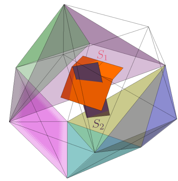
Figure 2. An example of the geometrical setting in Case (i). Graphics generated using Wolfram Mathematica${}^{\text{\copyright}}$.

we assume that $\overline{S}_{1}\neq\overline{S}_{2}$. For all $\bm{y}\in{S}_{1}$ such that $\bm{y}\notin\overline{S}_{2}$, there exists a ball $B_{r}(\bm{y})$ that does not intersect $\overline{S}_{2}$. Hence,

$$\bm{0}=[\bm{w}]_{B_{r}(\bm{y})\cap S_{1}}=[\bm{u}_{1}]_{B_{r}(\bm{y})\cap S_{1}}=\bm{g}_{1},$$

and this identity leads to a contradiction, as supp($\bm{g}_{1}$)=$\overline{S}_{1}$. We can repeat the same argument, switching the role of $S_{1}$ and $S_{2}$, to conclude that $\overline{S}_{1}=\overline{S}_{2}$. Therefore,

$$\bm{0}=[\bm{w}]_{S_{1}}=[\bm{w}]_{S_{2}}\Rightarrow[\bm{u}_{1}]_{S_{1}}=[\bm{u}_{2}]_{S_{2}}\Rightarrow\bm{g}_{1}=\bm{g}_{2}.$$

Next, we analyze Case (ii), see Figure 3.

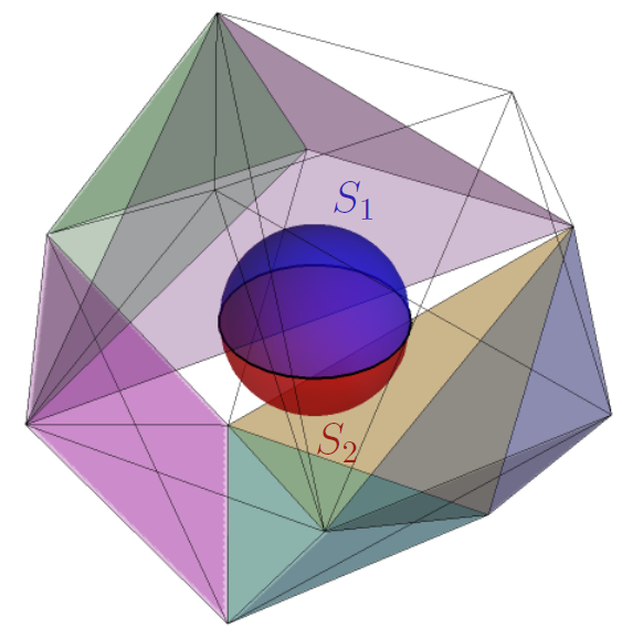
Figure 3. An example of the geometrical setting in Case (ii). Graphics generated using Wolfram Mathematica${}^{\text{\copyright}}$.

By Lemma 4.2, we can assume, without loss of generality, that there exists a bounded connected domain $D$ such that $\partial D=\overline{S_{1}\cup S_{2}}$. Then $\bm{w}=\bm{0}$ in a neighborhood of $\partial D$ in $\Omega\setminus\overline{D}$, since $\bm{w}=\bm{0}$ in $G$. The continuity of the tractions $(\mathbb{C}\widehat{\nabla}\bm{u}_{1})\bm{n}$ and $(\mathbb{C}\widehat{\nabla}\bm{u}_{2})\bm{n}$ in trace sense across $S_{1}$ and $S_{2}$, respectively, implies that

(36) $$(\mathbb{C}\widehat{\nabla}\bm{w}^{-})\bm{n}=\bm{0},$$

in $H^{-\frac{1}{2}}(\partial D)$ and hence a.e. on $\partial D$, where $\bm{w}^{-}$ indicates the function $\bm{w}$ restricted to $D$ and $\bm{n}$ the outward unit normal to $D$. Moreover, $\bm{w}^{-}$ satisfies

(37) $$\textrm{div}(\mathbb{C}\widehat{\nabla}\bm{w}^{-})=\bm{0}\,\quad\textrm{in}\,\,D.$$

We conclude from (36) and (37) that $\bm{w}^{-}$ is in the kernel of the operator for elastostatics in $H^{1}(D)$, i.e., it is a rigid motion:

$$\bm{w}^{-}=\mathbf{A}\bm{x}+\bm{c},$$

where $\bm{c}\in\mathbb{R}^{3}$ and $\mathbf{A}\in\mathbb{R}^{3\times 3}$ is a skew matrix. We conclude the proof by showing that this rigid motion can only be the trivial one. To this end, let $\mathcal{C}=\partial S_{1}\cap\partial S_{2}$. By construction $\bm{w}^{-}=[\bm{w}]_{S_{i}}=\bm{g}_{i}$ on $S_{i}$, so in particular it must vanish along $\partial S_{i}$, i.e., on $\mathcal{C}$ due to the hypothesis $\bm{g}_{i}\in H^{\frac{1}{2}}_{00}(S_{i})$. On the other hand the set of solutions of the linear system $\mathbf{A}\,\bm{x}=\bm{c}$, for any given $\bm{c}\in\mathbb{R}^{3}$ is a one-dimensional linear subspace of $\mathbb{R}^{3}$, since $\mathbf{A}$ is anti-symmetric, and therefore it cannot contain a closed curve. It follows that necessarily $\mathbf{A}=\mathbf{0}$ and $\bm{c}=\bm{0}$. Consequently, $\bm{w}^{-}=\bm{0}$ in $D$, hence $[\bm{w}]=\bm{0}$ on $\partial D$. In particular, $[\bm{w}]_{S_{1}}=\bm{0}=[\bm{u}_{1}]=\bm{g_{1}}\neq\bm{0}$, by the assumption that $\text{Supp}(\bm{g}_{i})=\overline{S_{i}}$. We reach a contradiction and, therefore, Case (ii) does not occur. ∎

References

- [1] M. S. Agranovich. Second-order strongly elliptic systems with boundary conditions on a nonclosed Lipschitz surface. Funktsional. Anal. i Prilozhen., 45(1):1–15, 2011.
- [2] M. S. Agranovich. Sobolev spaces, their generalizations and elliptic problems in smooth and Lipschitz domains. Springer Monographs in Mathematics. Springer, Cham, 2015. Revised translation of the 2013 Russian original.
- [3] G. Alessandrini, M. Di Cristo, A. Morassi, and E. Rosset. Stable determination of an inclusion in an elastic body by boundary measurements. SIAM J. Math. Anal., 46(4):2692–2729, 2014.
- [4] G. Alessandrini, L. Rondi, E. Rosset, and S. Vessella. The stability for the Cauchy problem for elliptic equations. Inverse Problems, 25(12):123004, 47, 2009.
- [5] P. F. Antonietti, F. Bonaldi, and I. Mazzieri. A high-order discontinuous Galerkin approach to the elasto-acoustic problem. Comput. Methods Appl. Mech. Engrg., 358:112634, 29, 2020.
- [6] P. F. Antonietti, A. Ferroni, I. Mazzieri, and A. Quarteroni. -version discontinuous Galerkin approximations of the elastodynamics equation. In Spectral and high order methods for partial differential equations—ICOSAHOM 2016, volume 119 of Lect. Notes Comput. Sci. Eng., pages 3–19. Springer, Cham, 2017.
- [7] T. Arnadottir and P. Segall. The 1989 loma-prieta earthquake imaged from inversion of geodetic data. Journal of Geophysical Research-solid Earth, 99(B11):21835–21855, 1994.
- [8] A. Aspri, E. Beretta, A. L. Mazzucato, and M. V. De Hoop. Analysis of a Model of Elastic Dislocations in Geophysics. Arch. Ration. Mech. Anal., 236(1):71–111, 2020.
- [9] E. Beretta, M. V. de Hoop, E. Francini, S. Vessella, and J. Zhai. Uniqueness and Lipschitz stability of an inverse boundary value problem for time-harmonic elastic waves. Inverse Problems, 33(3):035013, 27, 2017.
- [10] E. Beretta, E. Francini, A. Morassi, E. Rosset, and S. Vessella. Lipschitz continuous dependence of piecewise constant Lamé coefficients from boundary data: the case of non-flat interfaces. Inverse Problems, 30(12):125005, 18, 2014.
- [11] E. Beretta, E. Francini, and S. Vessella. Determination of a linear crack in an elastic body from boundary measurements—Lipschitz stability. SIAM J. Math. Anal., 40(3):984–1002, 2008.
- [12] E. Beretta, E. Francini, and S. Vessella. Uniqueness and Lipschitz stability for the identification of Lamé parameters from boundary measurements. Inverse Probl. Imaging, 8(3):611–644, 2014.
- [13] P. G. Ciarlet. Mathematical elasticity. Vol. I, volume 20 of Studies in Mathematics and its Applications. North-Holland Publishing Co., Amsterdam, 1988. Three-dimensional elasticity.
- [14] J. D. Eshelby. Dislocation theory for geophysical applications. Philosophical Transactions of the Royal Society A, 274(1239):331–338, 1973.
- [15] M. E. Gurtin. An introduction to continuum mechanics, volume 158 of Mathematics in Science and Engineering. Academic Press, Inc. [Harcourt Brace Jovanovich, Publishers], New York-London, 1981.
- [16] A. Hooper, D. Bekaert, K. Spaans, and M. Arikan. Recent advances in SAR interferometry time series analysis for measuring crustal deformation. Tectonophysics, 514:1–13, 2012.
- [17] O. A. Ladyzhenskaya and N. N. Ural’tseva. Linear and quasilinear elliptic equations. Translated from the Russian by Scripta Technica, Inc. Translation editor: Leon Ehrenpreis. Academic Press, New York-London, 1968.
- [18] C.-L. Lin, G. Nakamura, and J.-N. Wang. Optimal three-ball inequalities and quantitative uniqueness for the Lamé system with Lipschitz coefficients. Duke Math. J., 155(1):189–204, 2010.
- [19] J.-L. Lions and E. Magenes. Non-homogeneous boundary value problems and applications. Vol. III. Springer-Verlag, New York-Heidelberg, 1973. Translated from the French by P. Kenneth, Die Grundlehren der mathematischen Wissenschaften, Band 183.
- [20] S. E. Minson, M. Simons, and J. L. Beck. Bayesian inversion for finite fault earthquake source models I-theory and algorithm. Geophysical Journal International, 194(3):1701–1726, 2013.
- [21] J. Nečas. Les méthodes directes en théorie des équations elliptiques. Masson et Cie, Éditeurs, Paris; Academia, Éditeurs, Prague, 1967.
- [22] M. Nikkhoo, T. R. Walter, Paul R. Lundgren, and Pau Prats-Iraola. Compound dislocation models (CDMs) for volcano deformation analyses. Geophysical Journal International, 208(2):877–894, 2017.
- [23] Y. Okada. Internal deformation due to shear and tensile fault in a half-space. Bulletin of the Seismo-logical Society of America, 82(2):1018–1040, 1992.
- [24] O. A. Oleĭnik, A. S. Shamaev, and G. A. Yosifian. Mathematical problems in elasticity and homogenization, volume 26 of Studies in Mathematics and its Applications. North-Holland Publishing Co., Amsterdam, 1992.
- [25] S. Ozawa, T. Nishimura, H. Suito, T. Kobayashi, M. Tobita, and T. Imakiire. Coseismic and postseismic slip of the 2011 magnitude-9 Tohoku-Oki earthquake. Nature, 475(7356):373–U123, Jul 21 2011.
- [26] Y. Panara, G. Toscani, M. L. Cooke, S. Seno, and C. Perotti. Coseismic Ground Deformation Reproduced through Numerical Modeling: A Parameter Sensitivity Analysis. Geosciences, 9(9), 2019.
- [27] E. Rivalta, W. Mangiavillano, and M. Bonafede. The edge dislocation problem in a layered elastic medium. Geophysical Journal International, 149(2):508–523, 2002.
- [28] R. Sato. Crustal deformation due to a dislocation in a multi-layered medium. Journal of Physics of the Earth, 19(1):31–46, 1971.
- [29] P. Segall. Earthquake and Volcano Deformation. pages 1–432. Princeton University Press, 2010.
- [30] P. Segall and J. L. Davis. GPS applications for geodynamics and earthquake studies. Annual Review of Earth and Planetary Sciences, 25:301–336, 1997.
- [31] L. Tartar. An introduction to Navier-Stokes equation and oceanography, volume 1 of Lecture Notes of the Unione Matematica Italiana. Springer-Verlag, Berlin; UMI, Bologna, 2006.
- [32] F. Triki and D. Volkov. Stability estimates for the fault inverse problem. Inverse Problems, 35(7):075007, 20, 2019.
- [33] G. J. van Zwieten, R. F. Hanssen, and M. A. Gutiérrez. Overview of a range of solution methods for elastic dislocation problems in geophysics. Journal of Geophysical Research: Solid Earth, 118(4):1721–1732, 2013.
- [34] G.J. van Zwieten, E.H. van Brummelen, K.G. van der Zee, M.A. Guti̩rrez, and R.F. Hanssen. Discontinuities without discontinuity: The weakly-enforced slip method. Computer Methods in Applied Mechanics and Engineering, 271:144 Р166, 2014.
- [35] D. Volkov and J. Calafell Sandiumenge. A stochastic approach to reconstruction of faults in elastic half space. Inverse Probl. Imaging, 13(3):479–511, 2019.
- [36] D. Volkov, C. Voisin, and I. R. Ionescu. Reconstruction of faults in elastic half space from surface measurements. Inverse Problems, 33(5):055018, 27, 2017.
- [37] H. Yang. Recent advances in imaging crustal fault zones: a review. Earthquake Science, 28(2):151–162, 2015.
- [38] J. Zhang, Y. Bock, H. Johnson, P. Fang, S. Williams, J. Genrich, S. Wdowinski, and J. Behr. Southern California Permanent GPS Geodetic Array: Error analysis of daily position estimates and site velocities. Journal of Geophysical Research-Solid Earth, 102(B8):18035–18055, 1997.