1 Introduction

The GN model describes Dirac fermions with $N_{\mathrm{f}}$ flavors interacting via quartic interactions in $1+1$ dimensions. It was originally introduced as a toy model that shares several fundamental features with QCD [1]: it is renormalizable, asymptotically free, exhibits dynamical symmetry breaking of the $\mathbb{Z}_{2}$ chiral symmetry, and has a large $N_{\mathrm{f}}$ limit that behaves like the ’t Hooft large $N_{\mathrm{c}}$ limit of QCD. The particle spectrum and thermodynamics of the theory in the $N_{\mathrm{f}}\to\infty$ limit is known analytically. Similarly, the $1$-flavor model is equivalent to the $1$-flavor Thirring model which can be solved analytically in the massless limit [2] (it has a vanishing $\beta$-function). But for intermediate numbers of flavors $1<N_{\mathrm{f}}<\infty$ there is – despite many analytical and numerical studies – no complete understanding of the thermodynamics and particle spectrum.

The GN model and related four-Fermi theories in $1+1$ dimensions have been used in particle physics, condensed matter physics and quantum information theory. For example, in condensed matter physics the GN model describes the charge-soliton-conducting to metallic phase transition in polyacetylene (CH)_x as a function of a doping parameter [3]. It is equivalent to the Takayama-Lin-Liu-Maki model [4] which describes the electron-phonon interactions in CH in an effective low-energy continuum description, see Ref. [5]. The multi-flavor chiral GN model is related to the interacting Su-Schrieffer-Heeger model [6] which is used to investigate cold atoms in an optical lattice. Four-Fermi models are intensively studied to better understand and classify symmetry-protected topological phases of strongly interacting systems. For more details we refer to the nice summary in Ref. [7].

Recently we have seen a renewed interest in the physics of the GN model at low temperature and high baryon density, because it is the region of the QCD phase diagram which is particularly challenging for first-principles QCD approaches. Corresponding results are only available at asymptotically high densities, where the QCD coupling constant is small so that perturbation theory can be applied, at vanishing density, where lattice QCD does not suffer from the sign problem, or for unphysically large quark masses, where effective theories exist that mitigate the sign problem. At moderate densities and realistic values of the quark masses, i.e. the regime, which is probed by heavy-ion experiments and which is relevant for supernovae and compact stars, neither approach can be applied. In this regime our current picture of the QCD phase diagram is, thus, mostly based on QCD-inspired models, e.g. the GN model, the Nambu-Jona-Lasinio (NJL) model or the quark-meson model. In early calculations within these models it was assumed that the chiral condensate is homogeneous, i.e. constant with respect to the spatial coordinate(s). However, allowing for spatially varying condenates it turned out that there exist regions in the phase diagram, where inhomogeneous chiral phases are favored [8, 9]. The majority of the existing calculations have been performed in the limit $N_{\mathrm{f}}\rightarrow\infty$ or, equivalently, the mean-field approximation (see Ref. [10] for a review and Refs. [11, 12, 13, 14, 15, 16, 17, 18] for examples of recent work). Using lattice field theory and related numerical methods and considering $N_{\mathrm{f}}\rightarrow\infty$, the GN model has been explored in $1+1$ and $2+1$ dimensions, the chiral GN model in 1+1 dimensions and the NJL model in $1+1$ and $3+1$ dimension [19, 20, 21, 22, 23]. However, a full lattice simulation and investigation of the phase diagram of any of these models at finite number of fermion flavors, where quantum fluctuations are taken into account, is still missing. The main goal of the present work is to make a step in this direction and to explore, whether such inhomogeneous phases also exist in the $1+1$-dimensional GN model at finite $N_{\mathrm{f}}$.

In this work we shall use naive fermions and SLAC fermions to study the multi-flavor GN model. These fermion discretizations are all chiral and no fine tuning is required to end up with a chirally symmetric continuum limit. But the theorem of Nielsen and Ninomyia [24] tells us that we have to pay a price for using (strictly) chiral fermions. And indeed, with naive fermions we can only simulate $4,8,\dots$ flavors. With SLAC fermions we can simulate $1,2,\dots$ flavors, but the associated Dirac operator is non-local. It has been argued elsewhere that there is no problem with SLAC fermions for lattice systems without local symmetries, see for example Ref. [25]. We shall consider GN models with $2,8$ and $16$ flavors which have no sign-problem. The results for $8$ and $16$ flavors can be compared with the results obtained with naive fermions. We find full agreement of the results obtained with both fermion species. Note that with Wilson fermions the full chiral symmetry cannot be restored in the continuum limit with just one bare coupling. One needs to introduce a bare mass plus two bare couplings and fine tune these three parameters to arrive at a chirally symmetric continuum limit [26]. An alternative would be to use fermions which obey the Ginsparg-Wilson relation. We did not use such fermions, because we sample the full $\mu$-$T$ parameter space and carefully check for discretization and finite size effects. With Ginsparg-Wilson fermions this would be would be too time-consuming.

This paper is organized as follows. In section 2 we summarize some known features of the GN model that are relevant for its thermodynamical properties. These include properties of the fermion determinant in the continuum and on the lattice, homogeneous and inhomogeneous phases in the $N_{\mathrm{f}}\rightarrow\infty$ limit and some comments concerning the spontaneous symmetry breaking (SSB) of translation invariance. In section 3 we discuss different lattice discretizations, the scale setting and some details of the simulations. Our numerical results are presented in section 4. The main focus concerns the behavior of the two-point function of the order parameter for chiral symmetry breaking and the resulting consequences for the phase diagram in the plane spanned by the chemical potential $\mu$ and the temperature $T$. We shall see that the GN model with $N_{\mathrm{f}}=2$, $8$ and $16$ flavors behaves qualitatively similar to the model in the $N_{\mathrm{f}}\rightarrow$ limit. In particular we localize three regions in $\mu$-$T$ parameter space, where the two-point function shows a qualitatively different dependence on the spatial separation. The model with $N_{\mathrm{f}}=2$ is also simulated on rather large lattices with spatial extent $N_{s}$ up to $725$ lattice points to carefully investigate the long-range behavior of the correlator. In appendix A we discuss, why the lattice GN model with naive fermions may have an incorrect continuum limit, and how to modify the interaction term to end up with an (almost) naive fermion discretization with correct continuum limit.

2 Theoretical basics

2.1 The Gross-Neveu model

The Gross-Neveu model (GN model) is a relativistic quantum field theory describing $N_{\mathrm{f}}$ flavors of Dirac fermions with a four fermion interaction. In this work we investigate this asymptotically free model in 2 spacetime dimensions. The fermions are described by a field $\psi=(\psi_{1},\dots,\psi_{N_{\mathrm{f}}})$, the components of which are two-component Dirac spinors. Originally it has been studied in the $1/N_{\mathrm{f}}$ expansion. The action and partition function are

$$S_{\psi}=\int\mathrm{d}^{2}x\,\bigg{(}\bar{\psi}\mathrm{i}\not{\partial}\psi+\frac{g^{2}}{2N_{\mathrm{f}}}(\bar{\psi}\psi)^{2}\bigg{)}\,,\qquad Z=\int\mathcal{D}\bar{\psi}\mathcal{D}\psi\,\mathrm{e}^{-S_{\psi}}\,,$$ (1)

where the fermion bilinears contain sums over flavor indices, e.g. $\bar{\psi}\psi=\sum_{i}\bar{\psi}_{i}\psi_{i}$.

To be able to perform the fermion integration one follows Hubbard and Stratonovich by introducing a fluctuating auxiliary scalar field $\sigma$ to linearize the operator $\bar{\psi}\psi$ in the interaction term,

$$S_{\sigma}=\int\mathrm{d}^{2}x\,\bigg{(}\bar{\psi}\mathrm{i}D\psi+\frac{N_{\mathrm{f}}}{2g^{2}}\sigma^{2}\bigg{)}\,,\qquad Z=\int\mathcal{D}\bar{\psi}\mathcal{D}\psi\,\mathcal{D}\sigma\,e^{-S_{\sigma}}\,,$$ (2)

where

$$D=\not{\partial}+\sigma+\mu\gamma^{0}$$ (3)

is the Dirac operator. The four-Fermi term in (1) is recovered after eliminating $\sigma$ by its equation of motion or equivalently by integrating over $\sigma$ in the functional integral. In eqs. (2) and (3) we also introduced a chemical potential $\mu$ to study the system at finite fermion density. Expectation values of operators $\mathcal{O}(\psi,\bar{\psi},\sigma)$ in the grand canonical ensemble are given by

$$\langle\mathcal{O}\rangle=\frac{1}{Z}\int\mathcal{D}\bar{\psi}\mathcal{D}\psi\,\mathcal{D}\sigma\,\mathrm{e}^{-S_{\sigma}}\mathcal{O}(\psi,\bar{\psi},\sigma)\,.$$ (4)

Note that the integration is over fermion fields, which are anti-periodic in the Euclidean time direction, with period $\beta=1/T$, while the auxiliary scalar field is periodic.

Integrating over the fermion fields leads to

$$S_{\textrm{eff}}=\frac{1}{2g^{2}}\int d^{2}x\,\sigma^{2}-\log\det D\,,\qquad Z=\int\mathcal{D}\sigma\,e^{-N_{\mathrm{f}}S_{\textrm{eff}}}$$ (5)

with expectation values of operators $\mathcal{O}(\sigma)$ given by

$$\langle\mathcal{O}\rangle=\frac{1}{Z}\int\mathcal{D}\sigma\,\mathrm{e}^{-N_{\mathrm{f}}S_{\textrm{eff}}}\mathcal{O}(\sigma)\,.$$ (6)

Of particular interest in the present work is the chiral condensate, which distinguishes the different phases of the GN model. Translation invariance of the integral over $\mathrm{d}\sigma_{x}$ in the (well-defined) functional integral on the lattice implies a Ward-identity which states, that the condensate is proportional to the average auxiliary field,

$$\langle\bar{\psi}(\boldmathe{x})\psi(\boldmathe{x})\rangle=\frac{\mathrm{i}N_{\mathrm{f}}}{g^{2}}\langle\sigma(\boldmathe{x})\rangle\,,\qquad\boldmathe{x}=(x^{\mu})=\left(t\atop x\right)\,.$$ (7)

Also of interest is the Ward-identity relating the two-point function of the condensate to the two-point function of the auxiliary field,

$$\langle(\bar{\psi}\psi)(\boldmathe{x})(\bar{\psi}\psi)(\boldmathe{y})\rangle=\frac{N_{\mathrm{f}}}{g^{2}}\,\delta^{2}(\boldmathe{x}-\boldmathe{y})-\bigg{(}\frac{N_{\mathrm{f}}}{g^{2}}\bigg{)}^{2}\,\langle\sigma(\boldmathe{x})\sigma(\boldmathe{y})\rangle\,.$$ (8)

In our analysis of the phase diagram at finite temperature and density, the two-point function of the auxiliary field on the right hand side will play a crucial role (see section 4.3).

2.2 The fermion determinant

In this section we study some relevant spectral properties of the Euclidean Dirac operator $D$ with auxiliary field and chemical potential as defined in eq. (3).

Clearly, in the continuum the free massless Dirac operator $\not{\partial}=\gamma^{\mu}\partial_{\mu}$ and the partial derivatives $\partial_{\mu}$ have the following properties:

1. the differential operator $\not{\partial}$ is anti-hermitean and anti-commutes with $\gamma_{*}=\mathrm{i}\gamma^{0}\gamma^{1}$,

2. the partial derivatives $\partial_{\mu}$ are real, $\partial_{\mu}^{*}=\partial_{\mu}$.

Later on we shall discretize Euclidean spacetime on a lattice such that $\partial_{\mu}$ turns into a difference operator. For most discretizations one does not retain the above properties without introducing doublers – this is what the celebrated Nielsen-Ninomiya theorem tells us [24]. In the present work, however, we shall use chiral lattice fermions with the above properties, naive fermions (having doublers) and SLAC fermions. Now we investigate the spectral properties of the neither hermitian nor anti-hermitian operator $D$ with eigenvalue equation

$$D\psi=(\not{\partial}+\sigma+\mu\gamma^{0})\psi=\lambda\psi$$ (9)

in the continuum or on the lattice under the assumption that a) and b) hold true.

Charge conjugation: In $2$ Euclidean spacetime dimensions there exists a symmetric charge conjugation matrix $\mathcal{C}$ with $\mathcal{C}^{-1}\gamma^{\mu}\mathcal{C}=\gamma^{\mu T}$. Since the (Euclidean) $\gamma$-matrices are hermitian we have $\gamma^{\mu*}=\gamma^{\mu T}$, and property b) implies

$$D^{*}=\gamma^{\mu*}\partial_{\mu}+\sigma+\mu\gamma^{0*}=\mathcal{C}^{-1}D\,\mathcal{C}\,.$$ (10)

It follows that all non-real eigenvalues come in complex conjugated pairs $(\lambda,\lambda^{*})$ such that $\det D$ is real. Hence there is no sign problem for an even number of flavors, since then $(\det D)^{N_{\mathrm{f}}}$ is non-negative.

Chiral symmetry: The four-Fermi term breaks the $\textrm{U}_{A}(N_{\mathrm{f}})$ chiral symmetry of the kinetic term. But a discrete discrete $\mathbb{Z}_{2}$ chiral symmetry still remains under which $\bar{\psi}\psi$ and $\sigma$ change their signs. Under this discrete chiral symmetry the Dirac operator is conjugated with $\gamma_{*}=\mathrm{i}\gamma^{0}\gamma^{1}$:

$$\gamma_{*}D\gamma_{*}=-\not{\partial}+\sigma-\mu\gamma^{0}.$$ (11)

Since (on a finite lattice) the number of eigenvalues of $D$ is even, we conclude that the determinant is an even function of the auxiliary field,

$$(\det D)[\sigma,\mu]=(\det D)[-\sigma,\mu]\,.$$ (12)

Hermitean conjugation: The Dirac operator in eq. (9) is the sum of one anti-hermitean and two hermitean terms and

$$D^{\dagger}[\sigma,\mu]=-D[-\sigma,-\mu]\,.$$ (13)

Since the determinant is real (and the number of eigenvalues is even) it follows that $\det D$ is invariant under a simultaneous sign change of $\sigma$ and $\mu$,

$$(\det D)[\sigma,\mu]=(\det D)[-\sigma,-\mu]\,.$$ (14)

Together with (12) this leads to a determinant which is an even function of the chemical potential,

$$(\det D)[\sigma,\mu]=(\det D)[\sigma,-\mu]\,.$$ (15)

Note that for most lattice fermions not all of the above properties hold true, for example for Wilson fermions the $\mathbb{Z}_{2}$ chiral symmetry is explicitly broken.

2.3 Summary of existing results in large -$N_{\mathrm{f}}$ limit

Before 2003 most field-theoreticians and particle physicists took for granted that in thermal equilibrium translation invariance is realized such that the chiral condensate $\langle\bar{\psi}\psi\rangle$ is constant. Assuming translation invariance one can analytically determine the phase diagram of the GN model at finite temperature and fermion density in the large -$N_{\mathrm{f}}$ limit [27]. But in the condensed matter community it has been known for a while that the Peierls instability may trigger a breaking of translation invariance. This explains, for example, the inhomogenous Fulde-Ferrell-Larkin-Ovchinnikov equilibrium state for ultracold fermions [28, 29] (see [30] for a recent review). Subsequently it was shown that for $N_{\mathrm{f}}\to\infty$ the relativistic GN model exhibits an inhomogeneous condensate at low temperature and high density. In a series of interesting papers [8, 9] an explicit expression for the condensate in terms of Jacobi elliptic functions has been derived.

2.3.1 Homogeneous phases in large $N_{\mathrm{f}}$-limit

For $N_{\mathrm{f}}\to\infty$ the saddle point approximation to the functional integral with integrand
$\exp(-N_{\mathrm{f}}S_{\mathrm{eff}})$ in eq. (5) becomes exact. This means that the condensate $\langle\sigma\rangle$ is identical to the field $\sigma$ which minimizes $S_{\mathrm{eff}}$. In particular, if we assume translation invariance then we may minimize $S_{\mathrm{eff}}[\sigma]$ on the set of constant fields. But for a constant $\sigma$ the regularized action is proportional to the Euclidean spacetime volume,

$$S_{\mathrm{eff}}=(\beta L)\,U_{\mathrm{eff}},\quad U_{\mathrm{eff}}=\frac{1}{2g_{\Lambda}^{2}}\sigma^{2}-\frac{1}{\beta L}\log{\det}_{\Lambda}D\,.$$ (16)

We renormalize the theory such that the minimum of the effective potential at zero temperature and zero chemical potential is at some $\sigma_{0}>0$. This determines the bare coupling $g_{\Lambda}$ as function of the dimensional parameter $\sigma_{0}$ and the momentum-cutoff $\Lambda$,

$$\frac{1}{g_{\Lambda}^{2}}=\frac{1}{2\pi}\log\bigg{(}\frac{2\Lambda}{\sigma_{0}}\bigg{)}^{2}\,.$$ (17)

The renormalized potential has the simple form

$$U_{\mathrm{eff}}=\frac{\sigma^{2}}{4\pi}\Big{(}\log\frac{\sigma^{2}}{\sigma_{0}}-1\Big{)}-\frac{1}{\pi}\int_{0}^{\infty}\mathrm{d}k\;\frac{k^{2}}{\varepsilon_{k}}\,\bigg{(}\frac{1}{1+\mathrm{e}^{\beta(\varepsilon_{k}+\mu)}}+\frac{1}{1+\mathrm{e}^{\beta(\varepsilon_{k}-\mu)}}\bigg{)}$$ (18)

with one-particle energies $\epsilon_{k}=\sqrt{k^{2}+\sigma^{2}}$. In accordance with our previous discussion it is an even function of the auxiliary field and of the chemical potential.

The minimizing field as function of the temperature and chemical potential is depicted in Figure 1, left. Throughout the present work we use $\sigma_{0}$ to set the scale and thus measure the chemical potential, temperature and condensate field in units of $\sigma_{0}$. The phase diagram shows a symmetric phase with vanishing condensate and a broken phase with homogeneous condensate.

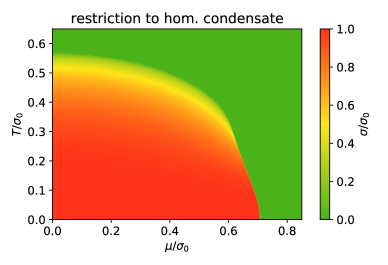
Figure 1: (left) The symmetric phase and the broken phase of the large-$N_{\mathrm{f}}$ GN model assuming a homogeneous condensate $\sigma$. The value of the condensate in units of $\sigma_{0}$ is color-coded. For large temperature or large chemical potential (the green region) the condensate vanishes. (right) The corrected phase diagram of the large-$N_{\mathrm{f}}$ GN model with homogeneous and inhomogeneous condensates. The first order line from the Lifshitz point to $T=0$ (red dashed line) obtained, when assuming a homogeneous condensate (see plot on the left side), turns into two second order lines (orange and green). In the region with large $\mu$ and low $T$ the condensate is inhomogeneous.

The system undergoes a phase transition from the symmetric phase at high temperature or large chemical potential to the broken phase at low $T$ and small $\mu$ [27, 31]. At vanishing chemical potential the transition happens at $T_{c}=e^{\gamma}/\pi\approx 0.567$. The second order line extends up to the Lifshitz point at $(\mu_{0},T)\approx(0.318,0.608)$, where it turns into a first order line. The latter intersects the zero-temperature axis at $\mu_{c}=1/\sqrt{2}\approx 0.707$. At $\mu_{c}$ and $T=0$ the condensate jumps from $1$ to $0$.

2.3.2 Inhomogeneous phase in large $N_{\mathrm{f}}$-limit

At low temperature and large chemical potential the minimum of $S_{\mathrm{eff}}$ does not correspond to a homogeneous but to a spatially inhomogeneous condensate $\langle\sigma(x)\rangle$. For a time-independent but spatially varying auxiliary field $\sigma$ the eigenfunctions of $D$ have the form $\psi_{nm}(\boldmathe{x})=e^{\mathrm{i}\omega_{n}t}\psi_{m}(x)$ with Matsubara frequency $\omega_{n}$. Summing over these frequencies in $\log\det D$ one arrives at the renormalized effective action

$$S_{\mathrm{eff}}[\sigma] =\frac{\beta L}{4\pi}\,{\hbox{\vbox{\hrule height=0.5pt\kern 2.15277pt\hbox{\kern-1.00006pt$\sigma$\kern-1.00006pt}}}}^{\,2}\Big{(}\log\frac{{\hbox{\vbox{\hrule height=0.5pt\kern 2.15277pt\hbox{\kern-1.00006pt$\sigma$\kern-1.00006pt}}}}^{\,2}}{\sigma_{0}^{2}}-1\Big{)}+\beta\Big{(}\sum_{n:\varepsilon_{m}<0}\varepsilon_{m}-\sum_{m:\bar{\varepsilon}_{m}<0}\bar{\varepsilon}_{m}\Big{)}$$

$$-\sum_{m:\varepsilon_{m}>0}\left(\log\big{(}1+e^{-\beta(\varepsilon_{m}+\mu)}\big{)}+\log\big{(}1+e^{-\beta(\varepsilon_{m}-\mu)}\big{)}\right)\,,$$ (19)

where the same renormalization prescription as in the homogeneous case has been adopted. The $\varepsilon_{m}$ are the real eigenvalues of the hermitean Dirac-Hamiltonian

$$h_{\sigma}\psi_{m}=\varepsilon_{m}\psi_{m},\qquad h_{\sigma}=\gamma^{0}\gamma^{1}\partial_{x}+\gamma^{0}\sigma$$ (20)

which appears in the decomposition

$$\gamma^{0}D=\partial_{0}+\mu+h_{\sigma}\,.$$ (21)

The $\bar{\varepsilon}_{m}$ are the eigenvalues of the Dirac Hamiltonian with constant auxiliary field $\bar{\sigma}$ given by

$${\bar{\sigma}}^{2}=\frac{1}{L}\int\mathrm{d}x\,\sigma^{2}(x)\,.$$ (22)

The two sums over the negative one-particle energies in the first line of (19) are easily identified as difference of two divergent vacuum energies: one for the prescribed auxiliary field $\sigma(x)$ and the other for the constant reference field  $\sigma$ defined in (22). A heat kernel regularization reveals that the first line in (19) is UV-finite if and only if the reference field is chosen as in (22). The $T$- and $\mu$- dependent traces in the second line in (19) are manifestly UV-finite and represent the finite temperature and density corrections.

In the large-$N_{\mathrm{f}}$ limit only auxiliary fields which minimize $S_{\mathrm{eff}}[\sigma]$ contribute to the functional integral in (2). With the Hellman-Feynman formula for the expectation values $\varepsilon_{m}=\langle\psi_{m}|h_{\sigma}|\psi_{m}\rangle$ the variational derivative of $S_{\mathrm{eff}}$ with respect to $\sigma$ can be calculated and one ends up with the Gap equation

$$\frac{1}{2\pi}\sigma(x)\log\frac{\bar{\sigma}^{2}}{\sigma_{0}^{2}} +\sum_{m:\varepsilon_{m}<0}\psi_{m}^{\dagger}(x)\gamma^{0}\psi_{m}(x)-\sum_{m:\bar{\varepsilon}_{m}<0}\bar{\psi}^{\dagger}_{m}(x)\gamma^{0}\bar{\psi}_{m}(x)$$

$$+\sum_{m:\varepsilon_{m}>0}\bigg{(}\frac{1}{1+e^{\beta(\varepsilon_{m}+\mu)}}+\frac{1}{1+e^{\beta(\varepsilon_{m}-\mu)}}\bigg{)}\psi_{m}^{\dagger}(x)\gamma^{0}\psi_{m}(x)=0\,.$$ (23)

This renormalized self-consistency equation is a complicated functional equation, whose solutions have been investigated at various times in the literature. Most derivations given previously derived the regularized gap equation from the regularized trace of the Green-function with bare coupling constant and cutoff parameter [32, 33, 34, 35]. Here the point of departure is the renormalized effective action (19) with physical scale parameter $\sigma_{0}$ and only finite quantities enter the derivation of the gap equation.

To summarize, to calculate the chiral condensate at finite temperature and finite density in the large-$N_{\mathrm{f}}$ limit one must solve the spectral problem for the $\sigma$-dependent Dirac Hamiltonian (20) and find a self-consistent solution $\sigma(x)$ of the gap equation (23). At zero temperature and fermion density Dashen et al. indeed could solve the coupled system for the modes $\psi_{n}(x)$ and the scalar field $\sigma(x)$ by using powerful inverse scattering methods [32]. They observed that a scalar field could only solve the gap equation if the solutions of the Dirac equation $\psi_{n}$ are not reflected. Their space-dependent solutions describe $n$-particle bound states with filled Dirac sea and masses

$$m_{B}=\frac{2\sigma_{0}}{\pi}\left(\frac{\sin\theta}{\theta}\right),\qquad\theta=\frac{n\pi}{2N_{\mathrm{f}}},\quad\quad n=2,\dots,N_{\mathrm{f}}-1\,.$$ (24)

Self-consistent solutions at finite temperature and fermion density have been constructed by Thies et al. [8, 9] by some (nonlinear) superposition of kink-antikink solutions. They succeeded to construct periodic solutions $\sigma(x)$ with associated Bloch waves $\psi_{n}(x)$ of the coupled system (20) and (23) in a certain region of the $(T,\mu)$ phase diagram. The Bloch waves (they are solutions of the Lamé equation) and the scalar field $\sigma(x)$ are given in terms of Jacobi’s elliptic functions, see Ref. [9]. The associated Dirac-Hamiltonian has one gap in the spectrum and the periodic and anti-periodic states at the band-edges are given by particular simple Jacobi functions. Thus, the property that $h_{\sigma}$ shows no reflection for baryon excitations above the vacuum is replaced by the property of having exactly one band gap in the spectrum if the system has high density.

In the large-$N_{\mathrm{f}}$ limit where the saddle point approximation to the functional integral (5) becomes exact the inhomogeneous condensate $\langle\sigma(x)\rangle$ minimizes the effective action (19) and thus is given by the solution of the gap equation, i.e. by a Jacobi elliptic function. For points in the phase diagram where the inhomogeneous solution has a lower effective action as any homogeneous solution the system is in a inhomogeneous phase. The correct phase diagram in the large-$N_{\mathrm{f}}$ limit is depicted in Figure 1, right. Note that the metastable phases and first order transition line (to guide the eye this line is kept as dashed line) disappear and are replaced by two second order transition lines. At low temperature and small chemical potential there is a homogeneous phase with broken chiral symmetry, at sufficiently high temperature we are in the homogeneous symmetric phase and at low temperature and large chemical potential we are in the inhomogeneous phase with an oscillating chiral condensate.

The wave length and amplitude of the condensate in the inhomogeneous phase are determined by the chemical potential or equivalently by the Fermi-momentum and by the temperature. If one moves within the inhomogeneous phase towards the symmetric phase, the amplitude of the condensate vanishes. If one moves towards the homogeneously broken phase, then the wave length of the condensate increases. In this work we mainly address the question whether there exists an inhomogeneous phase for a finite number of flavors $N_{\mathrm{f}}$ or whether such a phase is an artifact of the large-$N_{\mathrm{f}}$ limit.

2.4 Spontaneous breaking of a continuous symmetry in 1+1 dimensions

A well-known theorem by N. D. Mermin and H. Wagner in statistical mechanics states that a continuous symmetry cannot be spontaneously broken at finite temperature in 1- and 2-dimensional statistical systems with short range interaction [36]. A similar theorem has been proven by S. Coleman for relativistic quantum field theory in $d\leq 2$ dimensions [37]. Indeed, if spontaneous symmetry breaking of a continuous symmetry would occur, then as a consequence of the Goldstone theorem [38, 39] one would expect to find massless Nambu-Goldstone bosons (NGBs) in the particle spectrum. But massless scalars with a relativistic dispersion relation have an infrared divergent correlation function in lower dimensions and thus should not exist.

When proving the Goldstone theorem one makes basic assumptions: the theory should be Lorentz invariant, the Hilbert space should be positive and a global symmetry group $G$ should be broken to a subgroup $H$. Then there exists one massless scalar particle for each broken symmetry (or broken generator) such that there are $n_{\text{BG}}=\text{dim}(G/H)$ massless Goldstone bosons. In non-relativistic systems and for spacetime symmetries the situation is more intricate, since sometimes NGBs have unusual dispersion relations or they are even redundant.

• For example, in a ferromagnet and antiferromagnet we may have the same spontaneous symmetry breaking O(3)$\to$O(2), but in the first case we have only one NGB (the magnon) whereas in the second case there are two NGB. Since quantum field theories at high densities may be described by quasi-excitations with non-relativistic dispersion relations a similar reduction of NGB may happen in the high-density GN model.

• In addition, for a breaking of spacetime symmetries the simple counting rule does not apply. For example, crystals have phonons for spontaneously broken translations but no gapless excitations for equally spontaneously broken rotations. Again a reduction of the number of NGB may happen if we are dealing with spacetime symmetries instead of inner symmetries.

• Finally, it may happen that the NGB completely decouple from the rest of the system. Then one may evade the conclusion of Coleman’s theorem about the non-existence of NGB in $2$ spacetime dimensions. This seems to happen in the large $N_{\mathrm{f}}$-limit of the GN model [40], where translation invariance is definitely broken for high fermion density.

In 1976, Nielsen and Chadha [41] presented a general counting rule of NGBs valid either with or without relativistic invariance. They divided the modes into two classes, based on the behavior of their dispersion relations for small $|k|$:

$$\varepsilon_{k}\propto\begin{cases}\;|k|^{2n+1}&n\geq 0,\quad\text{type I}\\ \;|k|^{2n}&n>0,\quad\text{type II}\,.\end{cases}$$ (25)

Relativistic modes are of type I and non-relativistic modes are of type II. By examining analytic properties of correlation functions they showed that

$$n_{\text{NGB}}\leq n_{\text{BG}}\leq n_{\mathrm{I}}+2n_{\mathrm{II}}\,,$$ (26)

where $n_{\text{NGB}}$ is the total number of NGBs and $n_{\mathrm{I}}$ and $n_{\mathrm{II}}$ are the number of type I and type II NGBs. The number of broken generators $n_{\text{BG}}=\text{dim}(G/H)$ agrees with the number of “flat directions” of fluctuations of the order parameter.

In passing we note that there exists a related, but in general slightly different division of NGBs into type A and B [42, 43]. It is an algebraic classification based on the Lie algebra of symmetry generators. To each pair of non-commuting symmetry generators $\hat{Q}_{i},\hat{Q}_{j}$ (the conserved charges belonging to the symmetry group $G$) a NGB of type B is associated. The NGBs of type A tend to be linearly dispersive for small $|k|$. There is a simple counting for these NGBs:

$$n_{A}=n_{\text{BG}}-\text{rank}\,\rho,\quad n_{B}=\frac{1}{2}\text{rank}\,\rho\quad\text{such that}\quad n_{\text{NGB}}=n_{\text{BG}}-\frac{1}{2}\text{rank}\,\rho\,,$$ (27)

where $\rho$ is the Watanabe-Brauner matrix build from the conserved charges related to the symmetry group $G$, $\rho_{ij}\propto\langle[\hat{Q}_{i},\hat{Q}_{j}]\rangle$. For more details we refer to Refs. [44, 45].

Strictly speaking the above results hold for internal symmetries only. But it is believed that the NGBs originating from a spontaneously broken translation symmetry can be treated in essentially the same way as those associated with internal symmetries [44]. This leaves us with the following scenarios for the finite-temperature GN model at high density:

• Only the (abelian) spatial translation symmetry is broken such that the Watanabe-Brauner matrix $\rho$ vanishes. Then the results (27) would imply that there is just one type A NGB. If this would be – as expected – a NGB of type I with relativistic dispersion relation then we would be confronted with infrared divergences. The way out could be that it is not of type I but of type II or that it fully decouples from the system.

• Alternatively, if the above results do not apply to the breaking of translation invariance at high density systems, then we may as well find no NGB or a NGB of type II with non-relativistic dispersion relation $\varepsilon_{k}\sim|k|^{2}$. Its correlation function is not infrared divergent and the problem with the spontaneous breaking would go away.

Since the inhomogeneous condensate appears (at least in the large-$N_{\mathrm{f}}$ limit) at high density, a non-relativistic dispersion relation seems to be more likely than a relativistic one. Unfortunately, with the available ensembles on lattices of spatial extent up to $N_{s}=725$ lattice sites we cannot reliably measure the dispersion relation of the NGB (if it exists) in the model with $N_{\mathrm{f}}=2$ flavors in the infrared and thus cannot decide whether the NGB has a non-relativistic or a relativistic dispersion relation. It may even be that for finite $N_{\mathrm{f}}$ there is no SSB of translation invariance in the strict sense and that the model behaves like a simple atomic liquid, for example as liquid argon. Indeed, the correlator of the condensate on large lattices as presented in section 4 resembles the radial pair correlation function in an atomic fluid, see the reviews [46, 47]. In a forthcoming accompanying publication we will further substantiate, by studying the baryon number as function of the chemical potential, that the GN model at high density is either a crystal or an extremely viscous fluid.

3 Lattice field theory techniques

3.1 Notation

The number of lattice sites in temporal and spatial direction are denoted by $N_{t}$ and $N_{s}$, respectively. Consequently, the temperature is given by $T=1/N_{t}a$ and the extent of the periodic spatial direction by $L=N_{s}a$, where $a$ is the lattice spacing.

In the following we consider spacetime averages of observables $O[\sigma]$ for given field configurations $\sigma(\boldmathe{x})$ with $\boldmathe{x}=(t,x)$,

$$\hbox{\vbox{\hrule height=0.5pt\kern 2.15277pt\hbox{\kern-1.00006pt$O$\kern-1.00006pt}}}=\frac{1}{N_{t}N_{s}}\sum_{\boldmathe{x}}O[\sigma]\,.$$ (28)

We also compute ensemble averages,

$$\big{\langle}O\big{\rangle}=\frac{1}{N_{\textrm{conf}}}\sum_{\sigma}O[\sigma]\approx\frac{1}{Z}\int D\sigma\,e^{-S_{\textrm{eff}}[\sigma]}O[\sigma]\,,$$ (29)

where the sum over $\sigma$ extends over $N_{\textrm{conf}}$ field configurations $\sigma(\boldmathe{x})$ generated by Monte Carlo sampling according to $e^{-S_{\textrm{eff}}[\sigma]}$. The “$\approx$” sign in eq. (29) becomes the identity “$=$” in the limit $N_{\textrm{conf}}\rightarrow\infty$.

Moreover, we use the discrete Fourier transform either with respect to spacetime

$$\tilde{F}(\boldmathe{k})=\mathcal{F}(F)(\boldmathe{k})=\frac{1}{\sqrt{N_{t}N_{s}}}\sum_{t,x}e^{-\mathrm{i}\boldmathe{k}\cdot\boldmathe{x}}F(\boldmathe{x})\,,\qquad\boldmathe{k}=\left(\omega\atop k\right)$$ (30)

or space

$$\tilde{F}(k)=\mathcal{F}_{x}(F)(k)=\frac{1}{\sqrt{N_{s}}}\sum_{x}e^{-\mathrm{i}kx}F(x)\,,$$ (31)

with time and space restricted to the lattice sites, i.e.

$$\boldmathe{x}=a\boldmathe{m},\quad m_{0}=0,1,\dots,N_{t}-1,\quad m_{1}=0,1,\dots,N_{s}-1\,.$$ (32)

The corresponding momenta are

$$k_{0}\equiv\omega\in\left\{\frac{2\pi}{aN_{t}}n_{0}\right\},\quad k_{1}\equiv k\in\left\{\frac{2\pi}{aN_{s}}n_{1}\right\}\,.$$ (33)

For fermions we impose antiperiodic boundary conditions (BC) in $t$-direction such that the integer-spaced $n_{0}$ are half-integer valued. For bosons we impose periodic BC in $t$-direction such that the integer-spaced $n_{0}$ are integer valued. Both bosons and fermions are periodic in $x$-direction such that the integer-spaced $n_{1}$ are integer valued.

3.2 Lattice discretizations of fermions

We use two different lattice discretizations of fermions, naive fermions and SLAC fermions. Both discretizations have certain advantages but come also with subtleties, which are discussed in the following.

In section 4 we present numerical results for both discretizations and find agreement, which we consider an important cross check. Another comparison of the two discretizations can be found in section 3.2.3, where we show the $N_{\mathrm{f}}\rightarrow\infty$ phase diagram with the restriction to homogeneous condensate $\sigma$.

3.2.1 Naive fermions

The naive discretization is at first glance the most straightforward lattice discretization of fermions (see e.g. the textbooks [48, 49, 50]). In contrast to other common fermion discretizations, e.g. Wilson fermions, the free massless naive fermion action is chirally symmetric, which is an essential and necessary property in the context of this work. Naive fermions, however, lead to fermion doubling according to the Nielsen-Nynomia theorem [24]. Thus, for most applications, e.g. QCD with 2, 2+1 or 2+1+1 quark flavors, naive fermions are not appropriate. In our case of $1+1$ spacetime dimensions the number of fermion flavors is restricted to multiples of $4$. This is not a severe limitation, since we are not interested in a particular number of flavors $<4$, but mostly in simulating finite numbers of flavors, e.g. $N_{\mathrm{f}}=8$ or $N_{\mathrm{f}}=16$.

Besides fermion doubling there are, however, further pitfalls, which might lead to a continuum limit different from the theory of interest. In the context of the GN model, this was first observed and discussed in Ref. [51]. In appendix A we reproduce the arguments of Ref. [51] and we derive a modification of the straightforward naive discretization of the GN model, which has the correct continuum limit. This modified naive lattice action is

$$S_{\textrm{GN}}=\sum_{i=1}^{N_{\mathrm{f}}/4}S_{\textrm{free}}[\chi_{i},\bar{\chi}_{i}]+\frac{\mathrm{i}}{\sqrt{N_{t}N_{s}}}\sum_{i=1}^{N_{\mathrm{f}}/4}\sum_{\boldmathe{x},\boldmathe{y}}\bar{\chi}_{i}(\boldmathe{x})W(\boldmathe{x}-\boldmathe{y})\sigma(\boldmathe{y})\chi_{i}(\boldmathe{x})+\frac{N_{\mathrm{f}}}{2g^{2}}\sum_{\boldmathe{x}}\sigma^{2}(\boldmathe{x})$$ (34)

with the well-known action for naive free fermions coupled to a chemical potential

$$S_{\textrm{free}}[\chi,\bar{\chi}]=\sum_{\boldmathe{x}}\sum_{\nu=0,1}\frac{\mathrm{i}}{2a}\bar{\chi}(\boldmathe{x})\,\gamma^{\nu}\left(e^{a\mu\,\delta_{\nu 0}}\chi(\boldmathe{x}+a\boldmathe{e}_{\nu})-e^{-a\mu\,\delta_{\nu 0}}\chi(\boldmathe{x}-a\boldmathe{e}_{\nu})\right)$$ (35)

and the auxiliary field summed over neighbors with separation $a$ and $\sqrt{2}a$

$$\frac{1}{\sqrt{N_{t}N_{s}}}\sum_{\boldmathe{y}}W(\boldmathe{x}-\boldmathe{y})\sigma(\boldmathe{y})=\frac{1}{4}\sigma(\boldmathe{x})+\frac{1}{8}\sum_{\boldmathe{y}:|\boldmathe{y}-\boldmathe{x}|=a}\sigma(\boldmathe{y})+\frac{1}{16}\sum_{\boldmathe{y}:|\boldmathe{y}-\boldmathe{x}|=\sqrt{2}a}\sigma(\boldmathe{y})\,,$$ (36)

where $N_{\mathrm{f}}$ is a multiple of $4$ and $N_{t},N_{s}$ are even integers such that all doublers obey the same BC (for details see appendix A). For all computations with naive fermions presented in the following sections we use the action (34).

3.2.2 SLAC fermions

For SLAC-fermions the non-local derivatives in the Dirac operator are easily characterized in momentum space [54],

$$\mathcal{F}(\partial^{\mathrm{slac}}_{\mu}\psi)(\boldmathe{k})=\mathrm{i}k_{\mu}\mathcal{F}(\psi)(\boldmathe{k})$$ (37)

with the Fourier transform $\mathcal{F}$ as defined in eq. (30). We choose the discrete momenta $k_{\mu}$ symmetric to the origin to end up with a real and antisymmetric matrix $\partial_{\mu}$ [55]. This means that in spatial direction (with periodic BC) the lattice has an odd number $N_{s}$ of lattice sites, whereas in temporal direction (with antiperiodic BC) the lattice has an even number $N_{t}$ of lattice sites [50],

$$k_{0}=\frac{2\pi}{N_{t}a}n_{0}\quad,\quad n_{0}=\frac{N_{t}-1}{2},\frac{N_{t}-3}{2},\ldots,\frac{1-N_{t}}{2}\quad,\quad N_{t}\textrm{ even}$$

$$k_{1}=\frac{2\pi}{N_{s}a}n_{1}\quad,\quad n_{1}=\frac{N_{s}-1}{2},\frac{N_{s}-3}{2},\dots,\frac{1-N_{s}}{2}\quad,\quad N_{s}\textrm{ odd}.$$ (38)

Both the naive and the SLAC derivative define chiral fermions, for which $\mathrm{i}\not{\partial}$ is hermitean and anticommutes with $\gamma_{*}=\mathrm{i}\gamma^{0}\gamma^{1}$. In contrast to naive fermions, however, there are no doublers for SLAC-fermions. Thus they can be used to study any positive integer number of fermion flavors. We point out that the non-local SLAC-derivative must not be used in gauge theories, where the edge of the Brillouin zone (where $k_{\mu}$ jumps) is probed in the functional integral, which leads to a clash with Euclidean Lorentz invariance [56]. But SLAC-fermions have been successfully applied to non-gauge theories, for example scalar field theories [57], non-linear sigma models [58], supersymmetric Yukawa models [57] and more recently to interacting fermion systems [25].

For SLAC-fermions the chemical potential $\mu$ is introduced as in the continuum theory,

$$\bar{\psi}(x)\gamma_{0}\Big{(}\partial_{0}+\mu\Big{)}\psi(x)\ \ \rightarrow\ \ \bar{\psi}(x)\gamma_{0}\Big{(}\partial^{\mathrm{slac}}_{0}+\mu\Big{)}\psi(x).$$ (39)

Note that the chemical potential $\mu$ enters linearly and not via $\exp(\pm a\mu)$ multiplying a hopping term as e.g. for naive fermions (see e.g. eq. (35)) For some observables, for example the fermion density, this introduces an additional term $\propto\mu$ in the continuum limit, which can be easily subtracted, since (in $2$ spacetime dimensions) the term is finite and can be calculated analytically. We emphasize that this term is not a lattice artifact – it also exists in continuum theories when appropriate care is taken in manipulating divergent integrals [59]. After the subtraction is performed, results obtained with SLAC-fermions converge much faster to the continuum limit than for other fermion discretizations. A similar observation has been made when using a linear $\mu$ for naive fermions in $4$ spacetime dimensions [59]. All observables considered in the present work need no such subtraction.

3.2.3 Comparison of naive and SLAC fermions for $N_{\mathrm{f}}\rightarrow\infty$ and homogeneous condensate

In Figure 2 we show the $N_{f}\rightarrow\infty$ phase diagram with the restriction to a homogeneous condensate $\sigma$ for naive and for SLAC fermions. The corresponding computations are straightforward and computationally rather cheap, when using techniques similar to those discussed in Refs. [19, 20, 21]. For both discretizations we performed computations for several significantly different values of the lattice spacing, $a\approx 0.41/\sigma_{0}$ and $a\approx 0.20/\sigma_{0}$ (naive and SLAC) and $a\approx 0.10/\sigma_{0}$ (only naive), but similar spatial extent $L$. When decreasing the lattice spacing, the results obtained with each of the two discretizations approach the continuum result from Ref. [27]. Note, however, that discretization errors for SLAC fermions are almost negligible, i.e. significantly smaller than discretization errors for naive fermions.

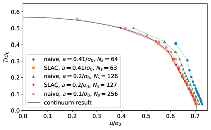
Figure 2: $N_{f}\rightarrow\infty$ phase diagram with the restriction to homogeneous condensate $\sigma$ for naive and for SLAC fermions (three different lattice spacings, $a\approx 0.41/\sigma_{0},0.20/\sigma_{0},0.10/\sigma_{0}$, similar spatial extent $L$). The solid grey line represents the continuum result from Ref. [27].

3.3 Simulation setup

We use a standard RHMC (Rational Hybrid Monte Carlo) algorithm [60] to perform numerical simulations. In detail we use the implementation described in Ref. [61], which was also used in Refs. [25, 62, 63].

3.3.1 Scale setting

We assume that at chemical potential $\mu=0$ and temperature $T=0$ the system is in a homogeneously broken phase and use the (positive) expectation value

$$\sigma_{0}=\lim_{L\rightarrow\infty}\langle\,\hbox{\vbox{\hrule height=0.5pt\kern 2.15277pt\hbox{\kern-1.00006pt$\sigma$\kern-1.00006pt}}}\,\rangle=\lim_{L\rightarrow\infty}\langle|\hskip 1.13809pt\hbox{\vbox{\hrule height=0.5pt\kern 2.15277pt\hbox{\kern-1.00006pt$\sigma$\kern-1.00006pt}}}\hskip 0.56905pt|\rangle\Big{|}_{\mu=0,T=0}$$ (40)

to set the scale. In other words, we express all dimensionful quantities in units of $\sigma_{0}$, e.g. we use for the chemical potential $\mu/\sigma_{0}$, for the temperature $T/\sigma_{0}$, etc. Setting the scale via $\sigma_{0}$ was also done in previous analytical and numerical studies of the phase diagram of the GN model in the $N_{\mathrm{f}}\rightarrow\infty$ limit (see e.g. [8, 9, 19, 20, 21]), i.e. expressing dimensionful quantities in units of $\sigma_{0}$ allows a straightforward comparison of our results at finite $N_{\mathrm{f}}$ to existing $N_{\mathrm{f}}\rightarrow\infty$ results.

The determination of $\sigma_{0}$ in lattice units is technically straightforward. When increasing the number of lattice sites in temporal direction $N_{t}$ as well as in spatial direction $N_{s}$ at fixed coupling $g^{2}$, the ensemble average $\langle|\hskip 1.13809pt\hbox{\vbox{\hrule height=0.5pt\kern 2.15277pt\hbox{\kern-1.00006pt$\sigma$\kern-1.00006pt}}}\hskip 0.56905pt|\rangle|_{\mu=0,T}$ quickly approaches the constant $\sigma_{0}$. Thus, in practice, one just has to compute $\langle|\hskip 1.13809pt\hbox{\vbox{\hrule height=0.5pt\kern 2.15277pt\hbox{\kern-1.00006pt$\sigma$\kern-1.00006pt}}}\hskip 0.56905pt|\rangle|_{\mu=0,T}$ on a lattice with sufficiently large $N_{t}$ and $N_{s}$, where $\langle|\hbox{\vbox{\hrule height=0.5pt\kern 2.15277pt\hbox{\kern-1.00006pt$\sigma$\kern-1.00006pt}}}|\rangle|_{\mu=0,T}\approx\sigma_{0}$. This is illustrated in Figure 3 for $N_{\mathrm{f}}=8$, SLAC fermions and two different $g^{2}$.

Figure 3: $a\langle|\hskip 1.13809pt\hbox{\vbox{\hrule height=0.5pt\kern 1.93748pt\hbox{\kern-0.90005pt$\sigma$\kern-0.90005pt}}}\hskip 0.56905pt|\rangle|_{\mu=0,T}$ as a function of $1/N_{t}=Ta$ for $\mu=0$, $N_{\mathrm{f}}=8$, SLAC fermions, two different $g^{2}$ and two different $N_{s}=L/a$. The plateau values at small $1/N_{t}$ correspond to $a\sigma_{0}$.

As e.g. in lattice simulations of 4-dimensional Yang-Mills theory or QCD, the lattice spacing $a$ is a function of the dimensionless coupling $g^{2}$ and can be set by choosing appropriate values for $g^{2}$. This is reflected by the two plateau values at small $1/N_{t}$ in Figure 3 representing $a\sigma_{0}$ (the lattice spacing in units of $\sigma_{0}$), which correspond to $g^{2}=0.192$ (larger lattice spacing) and $g^{2}=0.161$ (smaller lattice spacing).

3.3.2 Ensembles of field configurations

To explore the $\mu$-$T$ phase diagram of the $1+1$-dimensional GN model and its dependence on the number of fermion flavors $N_{\mathrm{f}}$ and to exclude sizable lattice discretization and finite volume corrections, we generated a large number of ensembles of field configurations $\sigma(\boldmathe{x})$. These ensembles are listed in Table 1.

$N_{\mathrm{f}}$	$N_{s}=L/a$	$N_{t}=1/Ta$	$\mu/\sigma_{0}$	$g^{2}$	$a\sigma_{0}$
SLAC, thermodynamics
$2$	$63$	$4,6,\dots,24,28,32,$ $40,\dots,64,80$	$0.0,\ldots,1.4$	$1.9569$	$0.4100(5)$
$8$	$31,47,63,127$	$4,6,\dots,24,28,32,$ $40,\dots,64,80$	$0.0,\ldots,1.4$	$1.5384$	$0.4100(5)$
				$1.2904$	$0.2495(5)$
				$1.1680$	$0.195(5)$
$16$	$63$	$4,6,\dots,24,28,32,$ $40,\dots,64\phantom{,80}$	$0$	$1.4953$	$0.4100(5)$
Naive, thermodynamics
$8$	$64$	$2,4,\dots,44,48,$ $52,\dots,64$	$0.0,\ldots,1.4$	$1.8132$	$0.4113(3)$
			$0.0,\ldots,1.1$	$1.4172$	$0.2518(5)$
	$128$	$100$	$0.7,0.9$	$1.0960$	$0.1253(3)$
SLAC, long-range behavior of the correlation function
$2$	$65,125,185,255,$ $375,525,725$	$80$	$0.5$	$1.9569$	$0.4100(5)$

Table 1: Ensembles of field configurations.

For given coupling $g^{2}$, i.e. for fixed lattice spacing $a$, we vary the temperature $T=1/N_{t}a$ by changing $N_{t}$, the number of lattice sites in temporal direction. Thus, at fixed $g^{2}$ the temperature $T$ can only be changed in discrete steps. The chemical potential $\mu$, on the other hand, is not restricted in such a way and can be set to any value.

The majority of simulations were carried out for $N_{\mathrm{f}}=8$:

• We simulated at several different spatial extents with $31\leq N_{s}\leq 128$ corresponding to $L=N_{s}a$ to check for finite volume corrections.

• We simulated at several different values of the coupling $g^{2}$ corresponding to four different lattice spacings $a\approx 0.41/\sigma_{0},0.25/\sigma_{0},0.20/\sigma_{0},0.13/\sigma_{0}$ (the lattice spacing is listed in units defined by $\sigma_{0}$ in the column “$a\sigma_{0}$” of Table 1).

• We simulated at many different values of the chemical potential, to explore the phase diagram.

• We carried out a sizable amount of these simulations using both fermion discretizations, i.e. SLAC fermions and naive fermions, to cross-check our results (the corresponding coupling constants $g^{2}$ have been tuned in such a way, that the simulated lattice spacings are almost identical).

Simulations at $N_{\mathrm{f}}=2$ and $N_{\mathrm{f}}=16$ were done with SLAC fermions, but not with naive fermions. For each ensemble between $300$ and $10\,000$ configurations were generated.

4 Numerical results

The majority of results shown in the following (section 4.2 to section 4.3) correspond to $N_{\mathrm{f}}=8$, the minimal number of flavors where computations are possible for both naive and SLAC fermions. Results for $N_{\mathrm{f}}=2$ and $N_{\mathrm{f}}=16$ are presented in section 4.4 and section 4.5.

4.1 Qualitative expectations

In the $1+1$-dimensional GN model in the limit $N_{\mathrm{f}}\rightarrow\infty$ there are three phases, a symmetric phase, a homogeneously broken phase and an inhomogeneous phase (see the discussion in section 2.3). The structure of the field configurations $\sigma(\boldmathe{x})$ generated during our simulations by the HMC algorithm suggest that there is a similar phase structure at finite $N_{\mathrm{f}}$. At large $T$ the field $\sigma(\boldmathe{x})$ mostly fluctuates around zero, while at small $T$ and small $\mu$ either $\sigma(\boldmathe{x})\approx+\sigma_{0}$ or $\sigma(\boldmathe{x})\approx-\sigma_{0}$. Most interestingly, however, at small $T$ and large $\mu$ the field $\sigma(\boldmathe{x})$ exhibits spatial periodic oscillations similar to a cos-function, which might signal an inhomogeneous phase. An example of a typical field configuration at $(\mu/\sigma_{0},T/\sigma_{0})\approx(0.450,0.030)$ with such periodic oscillations is shown in Figure 4.

Thus, we expect that the field configurations $\sigma(\boldmathe{x})$ generated by the Monte Carlo algorithm are crudely described by the following model:

• Inside a symmetric phase

  $$\sigma(\boldmathe{x})=\varepsilon\eta(\boldmathe{x})\,.$$ (41)

• Inside a homogeneously broken phase

  $$\sigma(\boldmathe{x})=\pm\,\zeta\sigma_{0}+\varepsilon\eta(\boldmathe{x})\,.$$ (42)

• Inside an inhomogeneous phase

  $$\sigma(\boldmathe{x})=A\cos\bigg{(}\frac{2\pi(x+\delta x)}{\lambda}\bigg{)}+\varepsilon\eta(\boldmathe{x})\,.$$ (43)

Figure 4: A typical field configuration $\sigma(\boldmathe{x})/\sigma_{0}$ generated by the HMC algorithm at large $\mu/\sigma_{0}\approx 0.450$ and small $T/\sigma_{0}\approx 0.030$, where an inhomogeneous phase is expected ($N_{\mathrm{f}}=8$, SLAC fermions, $a\approx 0.410/\sigma_{0}$, $N_{s}=127$). The clearly visible vertical stripes indicate six oscillations in spatial direction.

$\varepsilon\geq 0$, $\zeta>0$ and $A\geq 0$ are real parameters, which depend on $\mu$ and $T$. $\eta(\boldmathe{x})$ are independent continuous random variables with Gaussian probability distributions $p(\eta(\boldmathe{x}))\propto\exp(-\eta(\boldmathe{x})^{2}/2)$, which represent statistical fluctuations. $\lambda=L/(q+\delta q)$ is the wavelength of $\sigma$ in an inhomogeneous phase, where $q\geq 1$ is an integer parameter and $\delta q$ is an integer-valued discrete random variable with Gaussian probabilities $p(\delta q)\propto\exp(-\delta q^{2}/2\Delta q^{2})$. $\Delta q\ll q$, the width of the Gaussian, is another real parameter. $\delta x\in[0,L)$ is also a random variable, where it is a priori not clear, what kind of distribution to expect. The distribution could depend on the details of the HMC algorithm, and whether translation symmetry is spontaneously broken or not. Note, however, that the observables we are studying are constructed in such a way that they are independent of this distribution. To summarize, the model defined by eqs. (41) to (43) describes field configurations $\sigma(\boldmathe{x})$, which fluctuate around $0$ in a symmetric phase, around $\pm\zeta\sigma_{0}$ in a homogeneously broken phase and around a cos-function with varying wavelength $\lambda$ in an inhomogeneous phase.

With this model in mind, which is based on existing results in the $N_{\mathrm{f}}\rightarrow\infty$ limit [8, 9], we designed several observables, which are able to distinguish the three phases. Note that the sole purpose of this model is to provide some guidelines for the construction of observables and to develop expectations, in which way they characterize the three phases. The model is not used elsewhere in this work, in particular not for the analysis of our numerical results.

4.2 Squared spacetime average of $\sigma(\boldmathe{x})$

A rather simple observable is

$$\Sigma^{2}=\frac{\langle\hskip 1.13809pt\hbox{\vbox{\hrule height=0.5pt\kern 2.15277pt\hbox{\kern-1.00006pt$\sigma$\kern-1.00006pt}}}\hskip 0.56905pt^{2}\rangle}{\sigma_{0}^{2}},$$ (44)

the normalized ensemble average of the squared spacetime average of $\sigma(\boldmathe{x})$. It is not suited to characterize an inhomogeneous phase, but still useful to distinguish a homogeneously broken phase from a symmetric phase and an inhomogeneous phase. Note that our numerical results do not allow to decide, whether these regions in the $\mu$-$T$ plane are phases in a strict thermodynamical sense or rather regimes, which strongly resemble phases. In any case, throughout this paper we denote these regions as “phases”.

Within the model defined in section 4.1 one finds

• inside a symmetric phase

  $$\Sigma^{2}=\varepsilon^{2}/N_{t}N_{s}\sigma_{0}^{2}.$$ (45)

• inside a homogeneously broken phase

  $$\Sigma^{2}=\zeta^{2}+\varepsilon^{2}/N_{t}N_{s}\sigma_{0}^{2}.$$ (46)

• inside an inhomogeneous phase

  $$\Sigma^{2}=\varepsilon^{2}/N_{t}N_{s}\sigma_{0}^{2}.$$ (47)

Thus, we expect $\Sigma^{2}\approx 0$ both inside a chirally symmetric phase and inside an inhomogeneous phase, while it should be significantly larger, $\Sigma^{2}\approx 1$, inside a homogeneously broken phase.

In Figure 5 we show $\Sigma^{2}$ in the $\mu$-$T$ plane for naive fermions and SLAC fermions. The red regions clearly indicate a homogeneously broken phase, while the green regions represents a symmetric and/or an inhomogenous phase. The two plots are very similar. The main reason for the small discrepancies are lattice discretization errors, which are expected to be significantly larger for naive fermions than for SLAC fermions (see section 3.2.3). To ease comparison with $N_{\mathrm{f}}\rightarrow\infty$ results, we included the corresponding phase boundary of the homogeneously broken phase from Refs. [8, 9]. It is obvious that the homogeneously broken phase at finite $N_{\mathrm{f}}=8$ is of similar shape, but of smaller size than its analog at $N_{\mathrm{f}}\rightarrow\infty$. Such a reduction in size is expected, because at finite $N_{\mathrm{f}}$ there are fluctuations in $\sigma(\boldmathe{x})$, which increase disorder and, thus, favor a symmetric phase. Note that at small $T$ the boundary between the red and the green region starts to deviate significantly from the $N_{\mathrm{f}}\rightarrow\infty$ boundary and turns towards $(\mu,T)=(0,0)$. Our numerical results indicate that this is caused by the finite lattice spacing (see e.g. Figure 8). A qualitatively similar behavior was observed in an $N_{\mathrm{f}}\rightarrow\infty$ lattice study of the GN model [19].

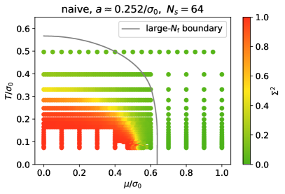
Figure 5: $\Sigma^{2}$ in the $\mu$-$T$ plane for naive fermions (left plot) and SLAC fermions (right plot) ($N_{\mathrm{f}}=8$). The red regions correspond to a homogeneously broken phase and the green regions to a symmetric and/or an inhomogenous phase. The gray lines represent the $N_{\mathrm{f}}\rightarrow\infty$ phase boundary of the homogeneously broken phase [8, 9].

4.3 The spatial correlation function of $\sigma(\boldmathe{x})$

In the limit $N_{\mathrm{f}}\rightarrow\infty$ in the inhomogeneous phase, $\sigma(\boldmathe{x})$ is a periodic function of the spatial coordinate $x$. It has a kink-antikink structure with large wavelength close to the boundary to the homogeneously broken phase and is sin-like with smaller wavelength for larger $\mu$. We expect a similar behavior also at finite $N_{\mathrm{f}}$ (see also eq. (43)).

Since the action $S_{\textrm{eff}}$ is invariant under spatial translations, field configurations, which are spatially shifted relative to each other, i.e. $\sigma(t,x)$ and $\sigma(t,x+\delta x)$, contribute with the same weight $e^{-S_{\textrm{eff}}}$ to the partition function and, thus, should be generated with the same probability by the HMC algorithm (see also the discussion on the distribution of $\delta x$ in section 4.1). Consequently, simple observables like $\langle\sigma(\boldmathe{x})\rangle$ are not suited to detect an inhomogeneous phase in a finite system, because destructive interference should lead to $\langle\sigma(\boldmathe{x})\rangle=0$ in a finite system, even in cases, where all field configurations exhibit spatial oscillations with the same wavelength. An observable, which does not suffer from destructive interference and is able to exhibit information about possibly present inhomogeneous structures, is the spatial correlation function of $\sigma(\boldmathe{x})$, i.e.

$$C(x)=\left\langle\sigma(t_{0},x)\sigma(t_{0},0)\right\rangle=\frac{1}{N_{t}N_{s}}\sum_{t,y}\big{\langle}\sigma(t,y+x)\sigma(t,y)\big{\rangle}\,.$$ (48)

The equality holds in thermal equilibrium and a finite box of length $L$ with periodic boundary conditions since $\langle\sigma(t,x+y)\sigma(t,y)\rangle$ does neither depend on $t$ nor on $y$. Actually, our HMC algorithm is able to sample all field configurations and, thus, to produce $y$-independent expectation values $\langle\sigma(t,x+y)\sigma(t,y)\rangle$. We use the sum over $t$ and $y$ in Eq. (48) to decrease statistical errors in the Monte Carlo average.

The correlator $C(x)$ is our main observable to detect and to distinguish the three expected phases, in particular an inhomogeneous phase. In contrast to the typical exponential decay of correlation functions, $C(x)$ is expected to oscillate in an inhomogeneous phase, i.e. $C(x)$ should be positive, if $x/\lambda$ is close to an integer, and negative, if $x/\lambda$ is close to a half-integer, where $\lambda$ denotes the wavelength of the spatial periodic structure of $\sigma(\boldmathe{x})$. Such oscillations are also found in the $N_{\mathrm{f}}\rightarrow\infty$ limit [65]. The expectation is also supported by analytical calculations within our model defined in section 4.1, where

• inside a symmetric phase

  $$C(x)=\varepsilon^{2}\delta_{x,0}$$ (49)

• inside a homogeneously broken phase

  $$C(x)=(\zeta^{2}\sigma_{0})^{2}+\varepsilon^{2}\delta_{x,0}$$ (50)

• inside an inhomogeneous phase

  $$\quad C(x)\approx\frac{A^{2}}{2}\frac{\vartheta(x/L,i/2\pi\Delta q^{2})}{\vartheta(0,i/2\pi\Delta q^{2})}\cos\bigg{(}\frac{2\pi qx}{L}\bigg{)}+\varepsilon^{2}\delta_{x,0}$$ (51)

with the Jacobi $\vartheta$ function

$$\vartheta(z,\tau)=1+2\sum_{n=1}^{\infty}e^{i\pi n^{2}\tau}\cos(2\pi nz)\,.$$ (52)

The cos-term in eq. (51) leads to oscillations with wave length $L/q$, while the factor including the $\vartheta$ function causes a damping of these oscillations for increasing separations $x$. This damping is due to the random fluctuations of the wave number $q+\delta q$ entering eq. (43) via $\lambda$, which cause destructive interference for larger $x$. The damping is strong for large fluctuations, i.e. large $\Delta q$, and not present in the limit $\Delta q\rightarrow 0$. Note that the result for $C(x)$ inside an inhomogeneous phase, i.e. the right hand side of eq. (51), is independent of the distribution of the random variable $\delta x$ introduced in section 4.1.

Of similar interest as $C(x)$ is its Fourier transform

$$\tilde{C}(k)=\mathcal{F}_{x}(C)(k)$$ (53)

(see eq. (31)). The expected behavior is the following:

• inside a symmetric phase $\tilde{C}(k)$ is rather small and smooth without any pronounced peak.

• inside a homogeneously broken phase $\tilde{C}(k)$ has a pronounced peak at $k=0$ and is rather small and smooth at $k\neq 0$.

• inside an inhomogeneous phase $\tilde{C}(k)$ has pronounced peaks at $k=\pm q$, where $q$ is related to the wavelength of the spatial oscillations of $C(x)$ via $\lambda=L/q$.

This expectation is in agreement with results obtained within our model from section 4.1, where

• inside a symmetric phase

  $$\tilde{C}(k)=\frac{1}{\sqrt{N_{s}}}\varepsilon^{2},$$ (54)

• inside a homogeneously broken phase

  $$\tilde{C}(k)=\sqrt{N_{s}}(\zeta\sigma_{0})^{2}\delta_{k,0}+\frac{1}{\sqrt{N_{s}}}\varepsilon^{2},$$ (55)

• inside an inhomogeneous phase

  $$\tilde{C}(k)\approx\frac{\sqrt{N_{s}}A^{2}}{4\vartheta(0,i/2\pi\Delta q^{2})}\bigg{(}\exp\bigg{(}-\frac{(k-q)^{2}}{2\Delta q^{2}}\bigg{)}+\exp\bigg{(}-\frac{(k+q)^{2}}{2\Delta q^{2}}\bigg{)}\bigg{)}+\frac{1}{\sqrt{N_{s}}}\varepsilon^{2}.$$ (56)

Exemplary results for $C(x)$ and $\tilde{C}(k)$ are shown in Figure 6 inside the symmetric phase
($(\mu/\sigma_{0},T/\sigma_{0})\approx(0,0.993)$), inside the homogeneously broken phase ($(\mu/\sigma_{0},T/\sigma_{0})\approx(0,0.083)$) and inside the inhomogeneous phase ($(\mu/\sigma_{0},T/\sigma_{0})\approx(0.700,0.083)$ and
$(\mu/\sigma_{0},T/\sigma_{0})\approx(0.900,0.083)$). In all cases there is reasonable agreement between our results for naive fermions and for SLAC fermions. Since lattice discretization errors are expected to be significantly larger for naive fermions, as discussed in section 3.2.3, we show results obtained with naive fermions in the inhomogeneous phase for two different lattice spacings, $a\approx 0.252/\sigma_{0}$ and $a\approx 0.126/\sigma_{0}$. Those corresponding to the finer lattice spacing are closer to the SLAC results, where $a\approx 0.250/\sigma_{0}$. We interpret this as indication that both discretizations agree in the continuum limit. Moreover, on a qualitative level there is agreement with our crude expectations summarized by eqs. (49) to (51) and eqs. (54) to (56), when the parameters in these equations are chosen appropriately. In particular the plots in the lower half of Figure 6 clearly indicate the existence of an inhomogeneous phase. $C(x)$ exhibits cos-like oscillations with decreasing wavelength $\lambda$ for increasing $\mu$, as observed in the $N_{\mathrm{f}}\rightarrow\infty$ limit. This is also reflected by the symmetric pair of peaks of $\tilde{C}(k)$ at the corresponding wave numbers $q=L/\lambda$. The gray curves in these plots represent the model expectations (eqs. (51) and (56)) with parameters $A$, $q$, $\Delta q$ and $\epsilon$ determined by fits to the lattice results for $C(x)$ and $\tilde{C}(k)$.

symmetric phase

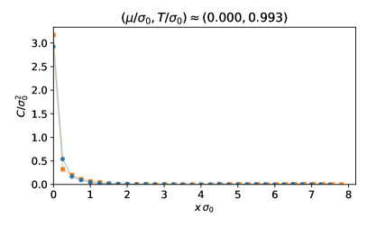
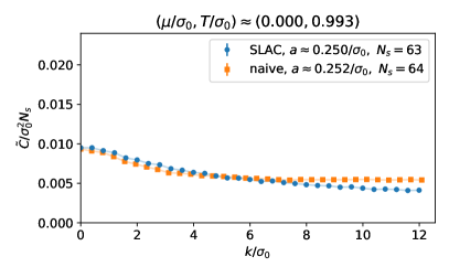
homogeneously broken phase

inhomogeneous phase

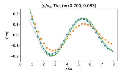
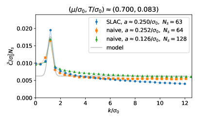
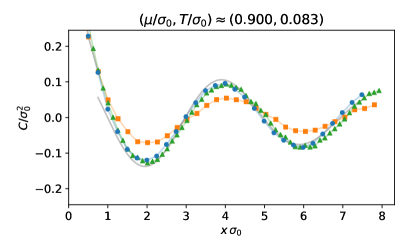
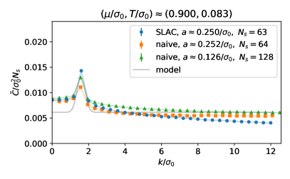
Figure 6: The spatial correlation function $C(x)/\sigma_{0}^{2}$ (left column, where the $x-$range extends to half the box length) and its Fourier transform $\tilde{C}(k)/\sigma_{0}^{2}N_{s}$ (right column) for SLAC fermions (blue dots) and naive fermions (orange and green dots) in the symmetric, the homogeneously broken and the inhomogeneous phase ($N_{\mathrm{f}}=8$) together with model expectations for the inhomogeneous phase (eqs. (51) and (56); gray curves).

A straightforward calculation leads to

$$\tilde{C}(k)=\bigg{\langle}\frac{1}{N_{t}\sqrt{N_{s}}}\sum_{t}|\tilde{\sigma}(t,k)|^{2}\bigg{\rangle}\,,$$ (57)

where

$$\tilde{\sigma}(t,k)=\mathcal{F}_{x}(\sigma)(t,k)$$ (58)

is the Fourier transform of $\sigma(\boldmathe{x})$ with respect to the spatial coordinate (see eq. (31)). The absolute values $|\tilde{\sigma}(t,k)|$ are invariant under spatial translations $x\rightarrow x+\delta x$, because

$$\mathcal{F}_{x}(\sigma(t,x+\delta x))(t,k)=e^{-\mathrm{i}k\delta x}\mathcal{F}_{x}(\sigma(t,x))(t,k).$$ (59)

This shows again that both $C(x)$ and $\tilde{C}(k)$ do not suffer from destructive interference, as already discussed at the beginning of this subsection. Moreover, eq. (57) shows in an explicit way that the Fourier transformed correlation function $\tilde{C}(k)$ also provides information about the absolute values of the Fourier coefficients of the field $\sigma(\boldmathe{x})$. In particular the peaks in $\tilde{C}(k)$ at non-vanishing $k$ in the plots in the lower half of Figure 6 indicate that inside an inhomogeneous phase strong oscillations with the same wavelength are present in the majority of the generated field configurations.

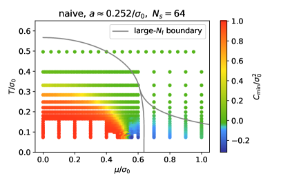
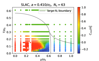
Figure 7: $C_{\textrm{min}}/\sigma_{0}^{2}$ in the $\mu$-$T$ plane for naive fermions (left plot) and SLAC fermions (right plot) ($N_{\mathrm{f}}=8$). The red regions correspond to a homogeneously broken phase, the green regions to a symmetric phase and the blue regions to an inhomogenous phase. The gray lines represent the $N_{\mathrm{f}}\rightarrow\infty$ phase boundaries [8, 9].

From Figure 6 one can see

$$C_{\textrm{min}}=\min_{x}\,C(x)\left\{\begin{array}[]{rl}\gg 0&\text{inside a homogeneously broken phase}\\ \approx 0&\text{inside a symmetric phase}\\ \ll 0&\text{inside an inhomogeneous phase}\end{array}\right.\,.$$ (63)

Thus, the minimum of the correlation function $C(x)$ is suited to plot a crude phase diagram as shown in Figure 7 both for naive and for SLAC fermions.

Figure 8: $C_{\textrm{min}}/\sigma_{0}^{2}$ in the $\mu$-$T$ plane for three different values of the lattice spacing $a$ (the columns) and four different numbers of lattice sites in spatial direction $N_{s}$ (the rows) ($N_{\mathrm{f}}=8$, SLAC fermions).

The red region indicates a homogeneously broken phase, the green region a symmetric phase and the blue region an inhomogeneous phase. As before, results obtained with these two different fermion discretizations are in fair agreement. Moreover, the phase diagram is qualitatively similar to the $N_{\mathrm{f}}\rightarrow\infty$ phase diagram from Refs. [8, 9], whose phase boundaries are also shown in Figure 7. The homogeneously broken phase and the inhomogeneous phase are, however, somewhat smaller for finite $N_{\mathrm{f}}$ than for $N_{\mathrm{f}}\rightarrow\infty$, presumably because quantum fluctuations at finite $N_{\mathrm{f}}$ increase disorder and, thus, favor a symmetric phase. Note, however, that $C_{\textrm{min}}$ is not the expectation value of a product of local operators as for example $C(x)$, which is the two-point function of the order parameter. In general one must be cautious, when using non-local quantities like $C_{\textrm{min}}$, since they can fake non-existing phase transitions [66, 67]. But in the present case transition lines have been localized by $C_{\textrm{min}}$ as well as the correlator $C(x)$ of the local field $\sigma$.

We also checked the stability of the phase diagram with respect to variations of the lattice spacing and the spatial volume. To this end we performed simulations using SLAC fermions at three different values of the lattice spacing, $a\approx 0.410/\sigma_{0},0.250/\sigma_{0},0.195/\sigma_{0}$ (the columns in Figure 8), and for four different numbers of lattice sites in spatial direction, $N_{s}=31,47,63,127$ (the rows in Figure 8). Approaching the infinite volume limit at fixed lattice spacing corresponds to moving from the top to the bottom of the figure, while approaching the continuum limit at approximately fixed spatial volume corresponds to moving right and downwards at the same time. There is little difference in the crude phase diagrams shown in these twelve plots. We consider this as indication that our results, at our current level of accuracy, are consistent with results in the continuum and infinite spatial volume.

      homogeneously broken $\leftrightarrow$ symmetric (blue points)

      inhomogeneous $\leftrightarrow$ symmetric (orange points)

                 

      homogeneously broken $\leftrightarrow$ inhomogeneous

Figure 9: $C_{\textrm{min}}/\sigma_{0}^{2}$ as function of $T$ for $\mu=0$ and for $\mu/\sigma_{0}\approx 0.600$ (left plot) and $C_{\textrm{min}}/\sigma_{0}^{2}$ as function of $\mu$ for $T/\sigma_{0}\approx 0.102$ (right plot) ($N_{\mathrm{f}}=8$, SLAC fermions, $a\approx 0.410/\sigma_{0}$, $N_{s}=63$).

In the limit $N_{\mathrm{f}}\rightarrow\infty$ the phase boundaries between the three phases are of second order. In the following we present selected results for finite $N_{\mathrm{f}}$ and discuss, whether there are also phase transitions or rather crossovers.

• For the transition between the symmetric and the homogeneously broken phase we computed $C_{\textrm{min}}$ as function of the temperature $T$ for vanishing chemical potential $\mu=0$ (see Figure 9, left plot, blue points). There is a rapid decrease of $C_{\textrm{min}}$ at around $T/\sigma_{0}=0.25$, which is qualitatively reminiscent to the $N_{\mathrm{f}}\rightarrow\infty$ result and, thus, might indicate that there is also a second order phase transition at finite $N_{\mathrm{f}}$.

• For the transition between the homogeneously broken and the inhomogeneous phase we computed $C_{\textrm{min}}$ as function of the chemical potential $\mu$ for rather low temperature $T/\sigma_{0}\approx 0.102$ (see Figure 9, right plot). We observe a rapid decrease of $C_{\textrm{min}}$ at around $\mu/\sigma_{0}=0.5$, which indicates a phase transition similar to the $N_{\mathrm{f}}\rightarrow\infty$ case.

• As can also be seen from the phase diagram in Figure 7, the transition between the symmetric and the inhomogeneous phase is somewhat washed-out. This is also reflected by Figure 9, left plot, where the orange points represent $C_{\textrm{min}}$ as function of the temperature $T$ for chemical potential $\mu/\sigma_{0}\approx 0.600$. These results favor a weak phase transition of second or higher order or just a crossover.

As has been pointed out earlier, these conclusions may not be fully coherent since $C_{\textrm{min}}$ is a non-local quantity.

4.4 The long-range behavior of $C(x)$

We have argued in section 2.4 that SSB of a continuous (spacetime) symmetry in $1+1$ dimensions is a delicate issue. To decide, whether there are NGB and if so, what type of NGB, we investigate the long-range correlations of the GN model with $N_{\mathrm{f}}=2$ flavors. The question is, whether the long-range order (which in the present context means that $C(x)$ oscillates with a constant non-zero amplitude for arbitrarily large $|x|$), which is necessary to form a crystal at $N_{\mathrm{f}}=\infty$, remains at finite $N_{\mathrm{f}}$ long-range or becomes almost long-range à la Berezinskii, Kosterlitz and Thouless (BKT) [68, 69] (in which case the amplitude decreases with distance like an inverse power). Indeed, by studying the long-range behavior of the SU$(N_{\mathrm{f}})$ Thirring model (this is a four-Fermi theory with current-current interaction) in $1+1$ dimensions, Witten argued that for finite $N_{\mathrm{f}}$ the correlations have almost long-range order,

$$\langle\bar{\psi}\psi(\boldmathe{x})\bar{\psi}\psi(0)\rangle\sim\frac{1}{|\boldmathe{x}|^{1/N_{\mathrm{f}}}}\,,\qquad|\boldmathe{x}|\to\infty\,,$$ (64)

such that only for $N_{\mathrm{f}}\to\infty$ the continuous chiral symmetry is broken, i.e. $\langle\bar{\psi}\psi\rangle\neq 0$ [70]. This way the system circumvents the no-go theorems for SSB of continuous inner symmetries. In what follows we try to answer the question whether a similar mechanism is at work for translation symmetry in the GN model.

To detect SSB of translation invariance directly we could break translation symmetry explicitly in a finite box with periodic BC, for example by adding a term $\varepsilon(x)\sigma(t,x)$ to the Lagrangian, perform the infinite volume limit and finally remove the source $\varepsilon(x)$. Assuming clustering in thermal equilibrium and

$$\lim_{\varepsilon\to 0}\lim_{L\to\infty}\langle\sigma(t,x)\sigma(t,0)\rangle_{\varepsilon}=\lim_{L\to\infty}\langle\sigma(t,x)\sigma(t,0)\rangle_{\varepsilon=0}=C(x)$$ (65)

we conclude that $C(x)$ is for large $|x|$ proportional to the condensate (calculated with first $L\to\infty$ and afterwards an adapted $\varepsilon\to 0$), i.e.

$$C(x)=\big{\langle}\sigma(t,x)\sigma(t,0)\big{\rangle}\to\big{\langle}\sigma(t,x)\big{\rangle}\big{\langle}\sigma(t,0)\big{\rangle}\quad\textrm{for}\quad|x|\to\infty\,.$$ (66)

In the inhomogeneous phase we can write

$$C(x)=A(x)C_{\mathrm{periodic}}(x)\,,$$ (67)

where $A(x)$ is the non-increasing amplitude function, while $C_{\mathrm{periodic}}(x)$ represents the periodic oscillations. If the system forms a crystal, the amplitude function $A(x)$ should approach a non-zero constant for sufficiently large separations $|x|$. In case the system has almost long-range order à la BKT, the amplitude function decreases with $|x|$ as an inverse power. To distinguish the two scenarios we study $C(x)$ for small $N_{\mathrm{f}}=2$, to detect a possible deviation of $A(x)$ from the asymptotically constant behavior in the large-$N_{\mathrm{f}}$ limit (for small $N_{\mathrm{f}}$ quantum fluctuations might be strong enough to change long-range into almost long-range order as it happens in the chirally invariant SU($N_{\mathrm{f}}$) Thirring model for finite $N_{\mathrm{f}}$ [70]). Thus, we expect one of the following amplitude functions:

1. In a BKT-like phase without SSB we expect the amplitude function $A(x)$ to have the following behavior for large $|x|$:

   $$A(x)=A_{\mathrm{BKT}}(x)\sim\frac{\alpha}{|x|^{\beta}}+\ldots$$ (68)

   The dots indicate sub-leading terms and terms arising from the finite spatial extent of the system.

2. If there is SSB of translation invariance, $C(x)$ oscillates with constant non-zero amplitude at large $|x|$, where the short-ranged contributions from excited states are suppressed. The amplitude function would then be

   $$A(x)=A_{\mathrm{SSB}}(x)\sim\gamma+\alpha e^{-m|x|}+\ldots\qquad\text{or}\qquad A(x)=A_{\mathrm{SSB^{\prime}}}(x)\sim\gamma+\frac{\alpha}{|x|^{\beta}}+\ldots$$ (69)

   depending on whether the excitations over the oscillating condensate are massive or massless. If the NGB decouple from the system, the amplitude function approaches the constant amplitude $\gamma\neq 0$ exponentially fast. If not, $A(x)$ will approach $\gamma\neq 0$ with an inverse power of $|x|$.

Before discussing the long-range behavior of $C(x)$ we present the phase diagram from $C_{\textrm{min}}$ for $N_{\mathrm{f}}=2$ in Figure 10. Again we recognize the same phases as in the large-$N_{\mathrm{f}}$ limit: a homogeneously broken phase which (as expected) is significantly smaller than for $N_{\mathrm{f}}=8$ and $N_{\mathrm{f}}\to\infty$, a symmetric phase for sufficiently large temperature and a region, where $C_{\textrm{min}}$ is clearly negative. One unexpected and striking feature of the latter phase is that the temperature range with negative $C_{\textrm{min}}$ grows with increasing $\mu$, which is qualitatively different from the situation at large $N_{\mathrm{f}}$. This already happens for $N_{\mathrm{f}}=8$ in a small region of parameter space (see Figure 8) but is so pronounced at $N_{\mathrm{f}}=2$ that up to $\mu/\sigma_{0}=1.4$ we found no evidence that the transition line separating the inhomogeneous and the restored phase will bend down to the $\mu$ axis.

Figure 10: $C_{\textrm{min}}/\sigma_{0}^{2}$ in the $\mu$-$T$ plane for $N_{\mathrm{f}}=2$. The red region corresponds to a homogeneously broken phase, the green region to a symmetric phase and the blue region to an inhomogenous phase. The grey lines represent the $N_{\mathrm{f}}\rightarrow\infty$ phase boundaries [8, 9].

Now we investigate the long-range behavior of the amplitude function $A(x)$ defined in eq. (67) for $N_{\mathrm{f}}=2$ on lattices with a rather large number of sites in spatial direction. Figure 11 shows the correlator $C(x)$ and its Fourier transform $\tilde{C}(k)$ for $(\mu/\sigma_{0},T/\sigma)=(0.500,0.030)$ and various $N_{s}$ up to $725$ corresponding to spatial extents up to $L\approx 297.3/\sigma_{0}$. We observe $32$ periods of statistically significant oscillations in $C(x)$ over the whole range of separations and a pronounced peak of $\tilde{C}(k)$ at the corresponding wave number. The position of the peak is essentially the same for all $L$ demonstrating once more that the wave length is independent of the spatial extent.

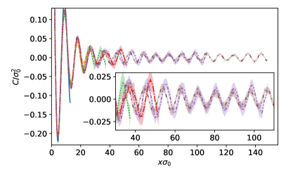
Figure 11: The spatial correlation function $C(x)/\sigma_{0}^{2}$ (left) and its Fourier transform $\tilde{C}(k)\sqrt{N_{s}}/\sigma_{0}^{2}$ (right) at $(\mu/\sigma_{0},T/\sigma)=(0.500,0.030)$ for $N_{\mathrm{f}}=2$ and $N_{s}=65,125,185,255,525,$ $725$. Except for the inset on the right, for clarity interpolating lines are shown instead of the data points.

The amplitude function $A(x)$ is extracted from the peaks of the correlation function $C(x)$ (which we identified using the scipy.signal.find_peaks method [71] with prominence=0.01) for all $N_{s}$, as exemplified for $N_{s}=725$ in the left plot of Figure 12. The peaks of $C(x)$ for various $N_{s}$ are depicted in the right plot of Figure 12. There is a rapid drop for small separations $x$ that flattens out for asymptotically large $x$. We performed $\chi^{2}$-minimizing fits of symmetrized versions of the expectations for the amplitude function $A(x)$ (eqs. (68) and (69)) to the extracted peaks for $N_{s}=725$ (see Figure 12, left plot). We only used data points with $x\geq x_{\min}$ in the fitting procedure, because all three fit functions are expected to model the amplitude function for large $|x|$. Since $\chi_{\textrm{red}}^{2}$ as a function of $x_{\min}$ is almost constant for large $|x|$ (see Figure 13, upper plot), we chose (independently for each of the three fits) the minimal value $x_{\min}$, where $\chi_{\textrm{red}}^{2}$ is consistent with the asymptotic constant, i.e. that value, where the constant behavior sets in. In the lower plot of Figure 13 we show the extracted parameters $\gamma$ appearing in the two fit functions in eq. (68) as functions of $x_{\min}$. It is reassuring that both parameters $\gamma$ are essentially independent of $x_{\min}$ as long as the corresponding $\chi_{\textrm{red}}^{2}$ is small. Since there are massive excitations in the SSB model and massless excitations in the SSB’ and BKT models, one should not expect to find the same $x_{\min}$ for the three models, but a smaller $x_{\min}$ for the SSB model, where the excitations are short-range. This expectation is confirmed by our numerical results (see column “$x_{\min}$” in Table 2).

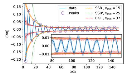
Figure 12: The left plot shows the correlation function $C(x)/\sigma_{0}^{2}$ at $(\mu/\sigma_{0},T/\sigma)=(0.500,0.030)$ for $N_{s}=725$, the extracted peaks and fits with the functions defined in eqs. (68) and (69) (the parameters obtained by these fits are shown in Table 2). For clarity interpolating lines are shown instead of the data points. The right plot shows the extracted peaks for $N_{s}=65,125,185,255,525,725$.

	$x_{\min}$	$\alpha$	$\beta$ resp. $m$	$\gamma$	$\chi_{\mathrm{red}}^{2}$
SSB	$15$	$0.231\pm 0.026$	$0.0895\pm 0.0054$	$0.00936\pm 0.00036$	$0.23$
SSB’	$25$	$\left(1.3\pm 2.2\right)\cdot 10^{3}$	$3.33\pm 0.50$	$0.00913\pm 0.00046$	$0.23$
BKT	$38$	$0.190\pm 0.082$	$0.66\pm 0.13$	-	$0.25$

Table 2: Parameters of the amplitude functions $A(x)$ in eqs. (68) and (69) obtained by fits to the extracted peaks for $N_{s}=725$.

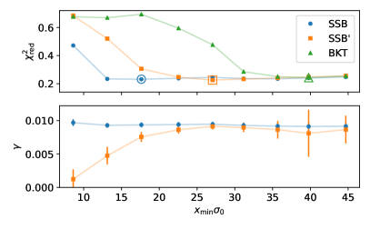
Figure 13: Top: $\chi_{\textrm{red}}^{2}$ as a function of $x_{\min}$ for all three models ($N_{s}=725$). Bottom: Extracted parameters $\gamma$ for the SSB and SSB’ model as functions of $x_{\min}$.

The fit results for the parameters of the amplitude functions $A(x)$ from eqs. (68) and (69) for $N_{s}=725$ are collected in Table 2. There are several points to note:

• The SSB model admits the most stable fits with resulting parameters almost independent of $x_{\min}$ and the initial values used in the fitting algorithm. $\gamma$ is cleary different from zero.

• Fits for the SSB’ model are less stable, which is reflected by the large uncertainties obtained for $\alpha$ and $\beta$. $\gamma$, however, can be determined in a reliable way and the result is again different from zero. Moreover, it is in excellent agreement with the corresponding result for the SSB model. It is also interesting to note that the SSB’ model, which differs from the BKT model by the additive constant $\gamma$, leads to significantly smaller $\chi_{\mathrm{red}}^{2}$ (and $\gamma\neq 0$) than the BKT model, when the same $x_{\min}$ is used.

• The BKT model is only able to describe the amplitude function for rather large $|x|$, i.e. the corresponding $x_{\min}$ is significantly larger than for the SSB model and SSB’ model. The fit result for the exponent is $\beta=0.66\pm 0.13$, which is similar to the corresponding analytically known value $\beta=1/N_{\mathrm{f}}=1/2$ of the $\textrm{SU}(N_{\mathrm{f}})$ Thirring model.

To summarize, it seems that the excitations are probably massive, because the SSB model is able to describe the extracted peaks for significantly smaller separations $x$, than it is possible with the SSB’ model or the BKT model. When allowing for a constant $\gamma$ (as in the SSB model and the SSB’ model), the fits lead to stable and clearly non-zero results. Thus, our current data is best described by the SSB scenario, where the NGB completely decouples from the system. However, this does not imply that this is the physical situation in the thermodynamic limit, since we saw that even $N_{s}=725$ lattice sites in spatial direction are not sufficient, to rule out the $1/|x|^{\beta}$ almost long-range behavior of the BKT scenario. In other words, a constant behavior $\propto\gamma$ and an inverse power $\propto 1/|x|^{\beta}$ are very similar for large $|x|$, in particular in a periodic spatial volume, such that even larger lattices or higher accuracy is needed to clearly distinguish between these scenarios.

Despite the fact that we could not fully reveal the nature of the inhomogeneous phase, we can still argue that there exists a phase transition between the inhomogeneous low-temperature phase and the symmetric high temperature phase. This can be seen from Figure 14, where we show the spatial correlation function $C(x)$ together with $\cosh$-fits for three different $(\mu,T)$ in the symmetric phase. It is evident that the $\cosh$-functions perfectly fit the data points, which indicates that in the symmetric phase the excitations are massive. In contrast to that, at low temperature in the inhomogeneous phase $C(x)$ is long-range or almost long-range (see Figure 11). Since $C(x)$ behaves qualitatively different in the inhomogeneous phase and in the symmetric phase, i.e. long-range or almost long-range versus exponentially decaying, we expect a phase transition, either a symmetry-restoring transition or a BKT-like transition from the low-temperature inhomogeneous phase to the high-temperature symmetric phase.

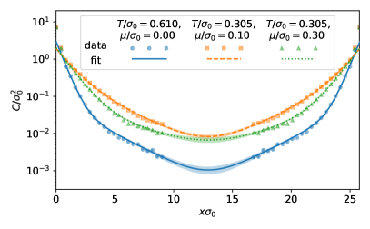
Figure 14: The spatial correlation function $C(x)/\sigma_{0}^{2}$ for three different $(\mu,T)$ in the symmetric phase and fits with $A_{1}\cosh(m_{1}(x-L/2))+A_{2}\cosh(m_{2}(x-L/2))$. We do not show data points in the region $9\leq x\sigma_{0}\leq 16$ because of large systematic errors due to autocorrelations.

4.5 Approaching the $N_{\mathrm{f}}\rightarrow\infty$ results with computations at finite $N_{\mathrm{f}}$

In sections 4.2 to 4.4 we have presented results at $N_{\mathrm{f}}=2$ and $N_{\mathrm{f}}=8$, which are similar to the analytically known $N_{\mathrm{f}}\rightarrow\infty$ results [8, 9], e.g. for the phase diagram. To check and to confirm that results at finite $N_{\mathrm{f}}$ approach for increasing $N_{\mathrm{f}}$ the $N_{\mathrm{f}}\rightarrow\infty$ results, we also performed simulations at $N_{\mathrm{f}}=16$. An exemplary plot is shown in Figure 15, where $\Sigma^{2}$ is shown as a function of the temperature $T$ for vanishing chemical potential $\mu=0$ and $N_{\mathrm{f}}=2,8,16,\infty$. While results for $N_{\mathrm{f}}=2$ agree with the $N_{\mathrm{f}}\rightarrow\infty$ result only for rather small $T/\sigma_{0}$, there is agreement also for larger $T/\sigma_{0}$, when $N_{\mathrm{f}}$ is increased, indicating that one can approach the analytically known $N_{\mathrm{f}}\rightarrow\infty$ results with computations at finite $N_{\mathrm{f}}$.

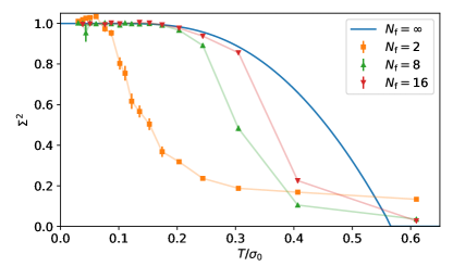
Figure 15: $\Sigma^{2}$ as a function of $T$ for $\mu=0$ and $N_{\mathrm{f}}=2,8,16,\infty$ (SLAC fermions, $a\approx 0.410/\sigma_{0}$, $N_{s}=63$).

5 Conclusions

In the present work we could localize three regimes in the space of thermodynamic control parameters $T$ and $\mu$, in which the two-point function of the order parameter shows qualitatively different behaviors. We spotted a homogeneously broken phase, a symmetric phase and a region with oscillating correlation function $C(x)$ defined in eq. (48). The results of our Monte Carlo simulations with two different types of chiral fermions for systems with $2$, $8$ and $16$ flavors on lattices with sizes up to $N_{t}=80$ and $N_{s}=725$ were presented, analyzed and discussed in the main body of the text. Although we could not answer the question, whether in GN models with a finite number of flavors translation invariance is spontaneously broken at low $T$ and large $\mu$, or whether the system is in a Berezinskii-Kosterlitz-Thouless like phase, we clearly spotted a low-temperature and high-density region, where the model exhibits oscillating spatial correlators. The wave-length of the spatial oscillation is determined by the chemical potential and temperature and not by the lattice spacing and the spatial extent of the lattice, i.e. spatial oscillations are neither a lattice artifact nor a finite size effect. We argued that there is a transition between the inhomogeneous phase and the symmetric phase which could be an infinite order transition (according to the Ehrenfest classification). In an accompanying paper we shall demonstrate that the ratio of the system size and the dominant wave length of the condensate oscillations is equal to the number of baryons in the systems. This further substantiates the physical picture that the GN model in equilibrium at low temperature and large fermion density either forms a crystal of baryons or a viscous fluid of baryons. In this work we also showed that the amplitude of oscillations stays constant or decays very slowly as suggested by a related result [70]. The first behavior is expected for a baryonic crystal the second behavior for a viscous baryonic fluid. To better understand, how the long range behavior at low temperature and high density does not clash with the absence of Nambu-Goldstone bosons in $1+1$ dimensions, needs further high-precision results on the two-point function of the order parameter. If the dispersion relation is non-relativistic or if the massless modes fully decouple from the system then there should be no problem.

Independent of whether the oscillating correlator $C(x)$ points to a baryonic crystal or a baryonic liquid for finite $N_{\mathrm{f}}$ we have seen that mean-field/large-$N_{\mathrm{f}}$ approximations may keep more information on the physics at finite $N_{\mathrm{f}}$ than one might expect. This is reassuring since in particle physics and even more so in solid state physics we often rely on mean-field type approximations. An important question is, of course, whether our results have any relevance for QCD at finite baryon density. On the one hand, we established that the interpretation as baryonic matter is not spoiled by taking quantum fluctuations into account. On the other hand, although recent numerical investigations of four-Fermi theories in $2+1$ dimensions and for $N_{\mathrm{f}}\to\infty$ spotted inhomogenous condensates [22], the spatial modulation is related to the cutoff scale and seems to disappear in the continuum limit [23]. Clearly, if this happens then we cannot expect a breaking of translation invariance for a finite number of flavors. Thus, extending our lattice studies to higher dimensions is of relevance for QCD. Simulations of interacting Fermi theories in $2+1$ dimensions are under way and we hope to report on our findings soon.

Appendix A Lattice discretization of the GN model with naive fermions

A.1 Free naive fermions

The action of free naive fermions with chemical potential $\mu$ is given in eq. (35). The Fourier representations of the fermion fields are

$$\chi(\boldmathe{x})=\frac{1}{\sqrt{N_{t}N_{s}}}\sum_{\boldmathe{k}}e^{\mathrm{i}\boldmathe{k}\cdot\boldmathe{x}}\tilde{\chi}(\boldmathe{k})\,,\qquad\bar{\chi}(\boldmathe{x})=\frac{1}{\sqrt{N_{t}N_{s}}}\sum_{\boldmathe{k}}e^{-\mathrm{i}\boldmathe{k}\cdot\boldmathe{x}}\tilde{\bar{\chi}}(\boldmathe{k})\,,$$ (70)

where the discrete $2$-momenta $\boldmathe{k}=(k_{0},k_{1})$ are in the first Brillouin zone, $-\pi\leq k_{\mu}a\leq\pi$, and are chosen such that BC in $t$ direction are antiperiodic and in $x$ direction are periodic (see section 3.1, in particular eq. (30)). Inserting these Fourier representations into eq. (35) leads to

$$S_{\textrm{free}}[\tilde{\chi},\tilde{\bar{\chi}}]=-\sum_{k}\tilde{\bar{\chi}}(k)\big{(}\gamma^{0}\mathaccent 28695{k}_{0}+\gamma^{1}\mathaccent 28695{k}_{1}\big{)}\tilde{\chi}(k)\,,$$ (71)

where we abbreviated

$$\mathaccent 28695{k}_{0}=\cosh(\mu a)\frac{\sin(k_{0}a)}{a}-\mathrm{i}\sinh(\mu a)\frac{\cos(k_{0}a)}{a}\,,\qquad\mathaccent 28695{k}_{1}=\frac{\sin(k_{1}a)}{a}\,.$$ (72)

In the limit $a\rightarrow 0$ the sums over $k_{0}$ and $k_{1}$ can be restricted to the “soft modes”, where both $|\mathaccent 28695{k}_{0}a|\ll 1$ and $|\mathaccent 28695{k}_{1}a|\ll 1$. There are four regions of soft modes in the first Brillouin zone, and they are denoted by $\mathcal{R}_{uv}$ with $u,v\in\{0,1\}$. The momenta of the soft modes in region $\mathcal{R}_{uv}$ are in the neighborhood of the four momenta

$$\boldmathe{k}_{uv}=\frac{\pi}{a}\left(u\atop v\right)\,,\qquad u,v\in\{0,1\}\,,$$ (73)

at which (for $\mu=0$) the lattice momenta $\mathaccent 28695{k}_{0}$ and $\mathaccent 28695{k}_{1}$ vanish. For $\boldmathe{k}\in\mathcal{R}_{uv}$ we have

$$\mathaccent 28695{k}_{0}=(-1)^{u}k_{0}-\mathrm{i}\mu+O(a^{2})\,,\qquad\mathaccent 28695{k}_{1}=(-1)^{v}k_{1}+O(a^{2})\,.$$ (74)

Now we define the soft modes in the four regions according to $\tilde{\chi}_{uv}(\boldmathe{k})=\tilde{\chi}(\boldmathe{k}_{uv}+\boldmathe{k})$ (and analogous for $\bar{\tilde{\chi}}$) with small $|k_{\mu}a|$. Neglecting the $O(a^{2})$ corrections in (74) we can approximate the free lattice action (71) by

$$S_{\textrm{free}}[\tilde{\chi},\tilde{\bar{\chi}}]\approx-\sum_{u,v}\sum_{\boldmathe{k}\in\mathcal{R}_{uv}}\tilde{\bar{\chi}}_{uv}(\boldmathe{k})\,\Big{(}\gamma^{0}((-1)^{u}k_{0}-\mathrm{i}\mu)+\gamma^{1}(-1)^{v}k_{1}\Big{)}\,\tilde{\chi}_{uv}(\boldmathe{k})\,.$$ (75)

This short calculation exhibits the well-known fermion flavor doubling for each spacetime dimension. It also shows that both $N_{t}$ and $N_{s}$ must be even to obey anti-periodic boundary conditions in $t$ direction and periodic boundary conditions in $x$ direction for each of the four fermion flavors.

It is important to note that the action (75) differs in a couple of minus signs in front of the $\gamma$ matrices for flavors $(u,v)\neq(0,0)$ from the corresponding continuum expression for four free fermion flavors. These minus signs can be eliminated by changing field coordinates via

$$\tilde{\chi}_{uv}=(\gamma^{0})^{u}(\gamma^{1})^{v}\tilde{\psi}_{uv}\,,\qquad\bar{\tilde{\chi}}_{uv}=\bar{\tilde{\psi}}_{uv}(\gamma^{1})^{v}(\gamma^{0})^{u}\,,\qquad u,v\in\{0,1\}\,.$$ (76)

Then eq. (75) becomes

$$S_{\textrm{free}}[\tilde{\psi},\tilde{\bar{\psi}}]\approx-\sum_{u,v}\ \sum_{\boldmathe{k}}\tilde{\bar{\psi}}_{uv}(\boldmathe{k})\big{(}\gamma^{0}(k_{0}-\mathrm{i}\mu)+\gamma^{1}k_{1}\big{)}\tilde{\psi}_{uv}(\boldmathe{k})\,.$$ (77)

This shows that the lattice action (35) corresponds in the continuum limit to four massless non-interacting fermion flavors.

A.2 Naive fermions and the GN model

Discretizing the GN model (2) with $N_{\mathrm{f}}=4$ flavors in a straightforward way using the fields $\chi$ and $\bar{\chi}$ via

$$S_{\sigma}[\chi,\bar{\chi},\sigma]=S_{\textrm{free}}[\chi,\bar{\chi}]+\mathrm{i}\sum_{\boldmathe{x}}\bar{\chi}(\boldmathe{x})\sigma(\boldmathe{x})\chi(\boldmathe{x})+\frac{N_{\mathrm{f}}}{2g^{2}}\sum_{\boldmathe{x}}\sigma^{2}(\boldmathe{x})\,,\qquad N_{\mathrm{f}}=4$$ (78)

actually results in a theory different from the GN model. To show this, we insert again the Fourier representations of the fermionic fields (70) as well as of the real scalar field $\sigma$,

$$\sigma(\boldmathe{x})=\frac{1}{\sqrt{N_{t}N_{s}}}\sum_{\boldmathe{k}}e^{\mathrm{i}\boldmathe{k}\cdot\boldmathe{x}}\,\tilde{\sigma}(\boldmathe{k})\,,$$ (79)

where $\tilde{\sigma}(-\boldmathe{k})={\tilde{\sigma}}^{\ast}(\boldmathe{k})$ and the discrete momenta $\boldmathe{k}$ are chosen such that $\sigma$ is periodic in $x^{0}$ and $x^{1}$ direction. The action (78) becomes

$$S_{\sigma}[\tilde{\chi},\tilde{\bar{\chi}},\tilde{\sigma}]=S_{\textrm{free}}[\tilde{\chi},\tilde{\bar{\chi}}]+\frac{\mathrm{i}}{\sqrt{N_{t}N_{s}}}\sum_{\boldmathe{k}}\sum_{\boldmathe{k}^{\prime}}\tilde{\bar{\chi}}(\boldmathe{k})\tilde{\sigma}(\boldmathe{k}-\boldmathe{k}^{\prime})\tilde{\chi}(\boldmathe{k}^{\prime})+\frac{N_{\mathrm{f}}}{2g^{2}}\sum_{\boldmathe{k}}\big{|}\tilde{\sigma}(\boldmathe{k})\big{|}^{2}\,,\qquad N_{\mathrm{f}}=4\,.$$ (80)

In the limit $a\rightarrow 0$ only the soft fermion modes contribute, as discussed in appendix A.1. Note, however, that there is no kinetic term for the field $\sigma$ and, thus, no corresponding suppression of $\sigma$ modes. Consequently, for $a\rightarrow 0$ the interaction term in eq. (80) can be written as

$$\frac{\mathrm{i}}{\sqrt{N_{t}N_{s}}}\sum_{\boldmathe{k},\boldmathe{k}^{\prime}}\sum_{u,v,u^{\prime},v^{\prime}}\bar{\tilde{\chi}}_{uv}(\boldmathe{k})\tilde{\sigma}_{uv,u^{\prime}v^{\prime}}(\boldmathe{k}-\boldmathe{k}^{\prime})\tilde{\chi}_{u^{\prime}v^{\prime}}(\boldmathe{k}^{\prime})\,,$$ (81)

with symmetric kernel in momentum space

$$\tilde{\sigma}_{uv,u^{\prime}v^{\prime}}(\boldmathe{k})=\tilde{\sigma}_{u^{\prime}v^{\prime},uv}(\boldmathe{k})=\tilde{\sigma}(\boldmathe{k}_{uv}-\boldmathe{k}_{u^{\prime}v^{\prime}}+\boldmathe{k})\,.$$ (82)

In terms of the usual field coordinates $\tilde{\psi}_{uv}$, related to $\tilde{\chi}_{uv}$ via eq. (76), the interaction term is

$$\frac{\mathrm{i}}{\sqrt{N_{t}N_{s}}}\sum_{\boldmathe{k},\boldmathe{k}^{\prime}}\sum_{u,v,u^{\prime}v^{\prime}}\bar{\tilde{\psi}}_{uv}(\boldmathe{k})(\gamma^{1})^{v}(\gamma^{0})^{u}\sigma_{uv,u^{\prime}v^{\prime}}(\boldmathe{k}-\boldmathe{k}^{\prime})(\gamma^{0})^{u^{\prime}}(\gamma^{1})^{v^{\prime}}\tilde{\psi}_{u^{\prime}v^{\prime}}(\boldmathe{k}^{\prime})\,.$$ (83)

Now it is obvious that the action (78) is not a discretization of the GN model with $N_{\mathrm{f}}=4$ fermion flavors. While the four terms with $uv=u^{\prime}v^{\prime}$ in eq. (83) represent the correct GN interaction for the four fermion flavors,

$$\frac{\mathrm{i}}{\sqrt{N_{t}N_{s}}}\sum_{u,v}\ \sum_{\boldmathe{k},\boldmathe{k}^{\prime}}\tilde{\bar{\psi}}_{uv}(\boldmathe{k})\tilde{\sigma}(\boldmathe{k}-\boldmathe{k}^{\prime})\tilde{\psi}_{u^{\prime}v^{\prime}}(\boldmathe{k}^{\prime}),$$ (84)

there are twelve additional terms not present in the GN model, where the field $\sigma$ couples two different fermion flavors,

$$\frac{\mathrm{i}}{\sqrt{N_{t}N_{s}}}\sum_{\boldmathe{k},\boldmathe{k}^{\prime}}\tilde{\bar{\psi}}_{10}(\boldmathe{k})\gamma^{0}\tilde{\sigma}(\pi/a+k_{0}-k_{0}^{\prime},k_{1}-k_{1}^{\prime})\tilde{\psi}_{00}(\boldmathe{k}^{\prime})+\text{eleven more terms}\,,$$ (85)

as was already pointed out in Ref. [51]. Including these twelve terms in a numerical simulation, i.e. using the action (78), corresponds to studying a different theory and leads to results significantly different from those obtained with a correct discretization of the GN model (examples are shown at the end of this section).

Figure 16: $\Sigma^{2}$ as a function of $T$ at $\mu=0$ for SLAC fermions, naive fermions and the straightforward, but incorrect naive discretization (78) ($N_{\mathrm{f}}=8$, $a\approx 0.410/\sigma_{0}$).

Now we derive a proper lattice discretization of the GN model. To this end, we note that only the soft fermion modes contribute in the limit $a\rightarrow 0$ and that the four correct interaction terms are proportional to $\tilde{\sigma}_{uv,uv}$, while the twelve spurious interaction terms are proportional to $\tilde{\sigma}_{uv,u^{\prime}v^{\prime}}$ with $uv\neq u^{\prime}v^{\prime}$. Thus, one can eliminate the spurious terms by replacing $\tilde{\sigma}(\boldmathe{k})$ in the interaction term in eq. (80) by $\tilde{W}(\boldmathe{k})\tilde{\sigma}(\boldmathe{k})$. Here $\tilde{W}$ is a weight-function with

• $\tilde{W}(\boldmathe{k})\rightarrow 1$ for $\boldmathe{k}\approx\boldmathe{k}_{00}=(0,0)$ (i.e. in region $\mathcal{R}_{00}$),

• $\tilde{W}(\boldmathe{k})\rightarrow 0$ for $\boldmathe{k}\approx\boldmathe{k}_{uv}$ with $(u,v)\neq(0,0)$ (i.e. in the other regions $\mathcal{R}_{uv}$).

A simple choice, which we use for our numerical simulations, is

$$\tilde{W}(\boldmathe{k})=\frac{1}{4}\prod_{\mu=0}^{1}\Big{(}1+\cos(ak_{\mu})\Big{)}\,.$$ (86)

Expressing this modified action in terms of $\chi(x)$, $\bar{\chi}(x)$ and $\sigma(x)$ is straightforward,

$$S_{\textrm{GN}}[\chi,\bar{\chi},\sigma]=S_{\textrm{free}}[\chi,\bar{\chi}]+\frac{\mathrm{i}}{\sqrt{N_{t}N_{s}}}\sum_{\boldmathe{x},\boldmathe{x}^{\prime}}\bar{\chi}(\boldmathe{x})W(\boldmathe{x}-\boldmathe{x}^{\prime})\sigma(\boldmathe{x}^{\prime})\chi(\boldmathe{x})+\frac{N_{\mathrm{f}}}{2g^{2}}\sum_{\boldmathe{x}}\sigma^{2}(\boldmathe{x})\,,\qquad N_{\mathrm{f}}=4\,,$$ (87)

where $W$ is the Fourier transform of $\tilde{W}$ and given in eq. (36). All calculations and arguments presented in this section apply to $N_{\mathrm{f}}=8,12,16,\ldots$ flavors in a trivial way. The generalization of eq. (87) is eq. (34).

In Figure 16 we show numerical evidence that using the straightforward naive discretization of the GN model (78) leads to incorrect results, i.e. results not corresponding to the GN model. We plot $\Sigma^{2}$ as a function of the temperature $T$ for chemical potential $\mu=0$. The blue and orange curves correspond to the SLAC discretization (see section 3.2.2) and the correct naive discretization (34) (or equivalently (87)). These curves are rather similar and get closer, when decreasing the lattice spacing, indicating that they have the same continuum limit. The green curve, on the other hand, corresponding to the straightforward naive discretization (78) is quite different and does not approach the blue and orange curves, when decreasing the lattice spacing. We obtained similar results also for non-vanishing chemical potenial.

References

- [1] D. J. Gross and A. Neveu, Dynamical Symmetry Breaking in Asymptotically Free Field Theories, Phys. Rev. D10 (1974) 3235.
- [2] I. Sachs and A. Wipf, Generalized Thirring models, Annals Phys. 249 (1996) 380, arXiv:hep-th/9508142.
- [3] A. Chodos and H. Minakata, The Gross-Neveu model as an effective theory for polyacetylene, Phys. Lett. A191 (1994) 39.
- [4] H. Takayama, Y. R. Lin-Liu and K. Maki, Continuum model for solitons in polyacetylene, Phys. Rev. B21 (1980) 2388.
- [5] H. Caldas, An Effective Field Theory Model for One-Dimensional Chains: Effects at Finite Chemical Potential, Temperature and External Zeeman Magnetic Field, J. Stat. Mech. 1110 (2011), no. 10 P10005, arXiv:1106.0948.
- [6] Y. Kuno, Phase structure of the interacting Su-Schrieffer-Heeger model and the relationship with the Gross-Neveu model on lattice, Phys. Rev. B99 (2019) 064105, arXiv:1811.01487.
- [7] A. Bermudez, E. Tirrito, M. Rizzi, M. Lewenstein and S. Hands, Gross-Neveu-Wilson model and correlated symmetry-protected topological phases, Annals Phys. 399 (2018) 149, arXiv:1807.03202.
- [8] M. Thies and K. Urlichs, Revised phase diagram of the Gross-Neveu model, Phys. Rev. D67 (2003) 125015, arXiv:hep-th/0302092.
- [9] O. Schnetz, M. Thies and K. Urlichs, Phase diagram of the Gross-Neveu model: Exact results and condensed matter precursors, Annals Phys. 314 (2004) 425, arXiv:hep-th/0402014.
- [10] M. Buballa and S. Carignano, Inhomogeneous chiral condensates, Prog. Part. Nucl. Phys. 81 (2015) 39, arXiv:1406.1367.
- [11] G. Basar, G. V. Dunne and M. Thies, Inhomogeneous Condensates in the Thermodynamics of the Chiral NJL(2) model, Phys. Rev. D79 (2009) 105012, arXiv:0903.1868.
- [12] D. Nickel, Inhomogeneous phases in the Nambu-Jona-Lasino and quark-meson model, Phys. Rev. D80 (2009) 074025, arXiv:0906.5295.
- [13] S. Carignano, D. Nickel and M. Buballa, Influence of vector interaction and Polyakov loop dynamics on inhomogeneous chiral symmetry breaking phases, Phys. Rev. D82 (2010) 054009, arXiv:1007.1397.
- [14] S. Carignano and M. Buballa, Two-dimensional chiral crystals in the NJL model, Phys. Rev. D86 (2012) 074018, arXiv:1203.5343.
- [15] A. Heinz, F. Giacosa and D. H. Rischke, Chiral density wave in nuclear matter, Nucl. Phys. A933 (2015) 34, arXiv:1312.3244.
- [16] J. Braun, F. Karbstein, S. Rechenberger and D. Roscher, Crystalline ground states in Polyakov-loop extended Nambu-Jona-Lasinio models, Phys. Rev. D93 (2016), no. 1 014032, arXiv:1510.04012.
- [17] M. Buballa and S. Carignano, Inhomogeneous chiral phases away from the chiral limit, Phys. Lett. B791 (2019) 361, arXiv:1809.10066.
- [18] S. Carignano and M. Buballa, Inhomogeneous chiral condensates in three-flavor quark matter, Phys. Rev. D101 (2020), no. 1 014026, arXiv:1910.03604.
- [19] P. de Forcrand and U. Wenger, New baryon matter in the lattice Gross-Neveu model, PoS LAT2006 (2006) 152, arXiv:hep-lat/0610117.
- [20] M. Wagner, Fermions in the pseudoparticle approach, Phys. Rev. D76 (2007) 076002, arXiv:0704.3023.
- [21] A. Heinz, F. Giacosa, M. Wagner and D. H. Rischke, Inhomogeneous condensation in effective models for QCD using the finite-mode approach, Phys. Rev. D93 (2016), no. 1 014007, arXiv:1508.06057.
- [22] M. Winstel, J. Stoll and M. Wagner, Lattice investigation of an inhomogeneous phase of the 2+1-dimensional Gross-Neveu model in the limit of infinitely many flavors (2019), arXiv:1909.00064.
- [23] R. Narayanan, Phase diagram of the large Gross-Neveu model in a finite periodic box (2020), arXiv:2001.09200.
- [24] H. B. Nielsen and M. Ninomiya, No Go Theorem for Regularizing Chiral Fermions, Phys. Lett. 105B (1981) 219.
- [25] B. H. Wellegehausen, D. Schmidt and A. Wipf, Critical flavor number of the Thirring model in three dimensions, Phys. Rev. D96 (2017), no. 9 094504, arXiv:1708.01160.
- [26] S. Aoki and K. Higashijima, The Recovery of the Chiral Symmetry in Lattice Gross-Neveu Model, Prog. Theor. Phys. 76 (1986) 521.
- [27] U. Wolff, The phase diagram of the inifinite N Gross-Neveu model at finite temperature and chemical potential, Phys. Lett. 157B (1985) 303.
- [28] P. Fulde and R. A. Ferrell, Superconductivity in a Strong Spin-Exchange Field, Phys. Rev. 135 (1964) A550.
- [29] A. I. Larkin and Y. N. Ovchinnikov, Nonuniform state of superconductors, Zh. Eksp. Teor. Fiz. 47 (1964) 1136.
- [30] J. J. Kinnunen, J. E. Baarsma, J.-P. Martikainen and P. Törmä, The Fulde-Ferrell-Larkin-Ovchinnikov state for ultracold fermions in lattice and harmonic potentials: a review, Rept. Prog. Phys. 81 (2018), no. 4 046401, arXiv:1706.07076.
- [31] A. Barducci, R. Casalbuoni, M. Modugno, G. Pettini and R. Gatto, Thermodynamics of the massive Gross-Neveu model, Phys. Rev. D51 (1995) 3042, arXiv:hep-th/9406117.
- [32] R. F. Dashen, B. Hasslacher and A. Neveu, Semiclassical Bound States in an Asymptotically Free Theory, Phys. Rev. D12 (1975) 2443.
- [33] R. Pausch, M. Thies and V. L. Dolman, Solving the Gross-Neveu model with relativistic many body methods, Z. Phys. A338 (1991) 441.
- [34] J. Feinberg, All about the static fermion bags in the Gross-Neveu model, Annals Phys. 309 (2004) 166, arXiv:hep-th/0305240.
- [35] G. Basar and G. V. Dunne, Self-consistent crystalline condensate in chiral Gross-Neveu and Bogoliubov-de Gennes systems, Phys. Rev. Lett. 100 (2008) 200404, arXiv:0803.1501.
- [36] N. D. Mermin and H. Wagner, Absence of ferromagnetism or antiferromagnetism in one-dimensional or two-dimensional isotropic Heisenberg models, Phys. Rev. Lett. 17 (1966) 1133.
- [37] S. R. Coleman, There are no Goldstone bosons in two-dimensions, Commun. Math. Phys. 31 (1973) 259.
- [38] J. Goldstone, Field Theories with Superconductor Solutions, Nuovo Cim. 19 (1961) 154.
- [39] Y. Nambu, Axial vector current conservation in weak interactions, Phys. Rev. Lett. 4 (1960) 380.
- [40] S.-S. Shei, Semiclassical Bound States in a Model with Chiral Symmetry, Phys. Rev. D14 (1976) 535.
- [41] H. B. Nielsen and S. Chadha, On How to Count Goldstone Bosons, Nucl. Phys. B105 (1976) 445.
- [42] H. Watanabe and T. Brauner, On the number of Nambu-Goldstone bosons and its relation to charge densities, Phys. Rev. D84 (2011) 125013, arXiv:1109.6327.
- [43] H. Watanabe and H. Murayama, Unified Description of Nambu-Goldstone Bosons without Lorentz Invariance, Phys. Rev. Lett. 108 (2012) 251602, arXiv:1203.0609.
- [44] H. Watanabe, Counting Rules of Nambu-Goldstone Modes, Ann. Rev. Condensed Matter Phys. 11 (2020) 169, arXiv:1904.00569.
- [45] M. Ammon, M. Baggioli and A. Jiménez-Alba, A Unified Description of Translational Symmetry Breaking in Holography, JHEP 09 (2019) 124, arXiv:1904.05785.
- [46] J. A. Barker and D. Henderson, What is ’liquid’? Understanding the states of matter, Rev. Mod. Phys. 48 (1976) 587.
- [47] D. Chandler, Introduction to modern statistical mechanics, Oxford University Press, New York (1987).
- [48] H. J. Rothe, Lattice Gauge Theories, World Scientific, 4th edn. (2012).
- [49] J. Smit, Introduction to quantum fields on a lattice: A robust mate, Cambridge Lect. Notes Phys. 15 (2002) 1.
- [50] A. Wipf, Statistical Approach to Quantum Field Theory, Lecture Notes in Physics 864 (2013).
- [51] Y. Cohen, S. Elitzur and E. Rabinovici, A Monte Carlo study of the Gross-Neveu model, Nucl. Phys. B220 (1983) 102.
- [52] L. Pannullo, J. Lenz, M. Wagner, B. Wellegehausen and A. Wipf, Inhomogeneous phases in the 1+1 dimensional Gross-Neveu model at finite number of fermion flavors, Acta Phys. Polon. Supp. 13 (2020) 127, arXiv:1902.11066.
- [53] L. Pannullo, J. Lenz, M. Wagner, B. Wellegehausen and A. Wipf, Lattice investigation of the phase diagram of the 1+1 dimensional Gross-Neveu model at finite number of fermion flavors, in 37th International Symposium on Lattice Field Theory (Lattice 2019) Wuhan, Hubei, China, June 16-22, 2019 (2019) arXiv:1909.11513.
- [54] S. D. Drell, M. Weinstein and S. Yankielowicz, Variational Approach to Strong Coupling Field Theory. 1. Phi**4 Theory, Phys. Rev. D14 (1976) 487.
- [55] G. Bergner, T. Kaestner, S. Uhlmann and A. Wipf, Low-dimensional Supersymmetric Lattice Models, Annals Phys. 323 (2008) 946, arXiv:0705.2212.
- [56] L. H. Karsten and J. Smit, The Vacuum Polarization With SLAC Lattice Fermions, Phys. Lett. 85B (1979) 100.
- [57] C. Wozar and A. Wipf, Supersymmetry Breaking in Low Dimensional Models, Annals Phys. 327 (2012) 774, arXiv:1107.3324.
- [58] R. Flore, D. Korner, A. Wipf and C. Wozar, Supersymmetric Nonlinear O(3) Sigma Model on the Lattice, JHEP 11 (2012) 159, arXiv:1207.6947.
- [59] R. V. Gavai and S. Sharma, Divergences in the quark number susceptibility: The origin and a cure, Phys. Lett. B749 (2015) 8, arXiv:1406.0474.
- [60] M. A. Clark and A. D. Kennedy, The RHMC algorithm for two flavors of dynamical staggered fermions, Nucl. Phys. Proc. Suppl. 129 (2004) 850, arXiv:hep-lat/0309084.
- [61] B. H. Wellegehausen, Phase diagrams of exceptional and supersymmetric lattice gauge theories, Ph.D. thesis, University Jena (2012).
- [62] J. J. Lenz, B. H. Wellegehausen and A. Wipf, Absence of chiral symmetry breaking in Thirring models in 1+2 dimensions, Phys. Rev. D100 (2019), no. 5 054501, arXiv:1905.00137.
- [63] D. August, M. Steinhauser, B. H. Wellegehausen and A. Wipf, Mass spectrum of -dimensional super Yang-Mills theory on the lattice, JHEP 01 (2019) 099, arXiv:1802.07797.
- [64] F. Karsch, J. B. Kogut and H. W. Wyld, The Gross-Neveu Model at Finite Temperature and Density, Nucl. Phys. B280 (1987) 289.
- [65] M. Thies (2019), unpublished notes.
- [66] J. Kertesz, Existence of weak singularities when going around the liquid-gas critical point, Physica A 58 (1989) 58.
- [67] S. Wenzel, E. Bittner, W. Janke, A. M. J. Schakel and A. Schiller, Kertesz line in the three-dimensional compact U(1) lattice Higgs model, Phys. Rev. Lett. 95 (2005) 051601, arXiv:cond-mat/0503599.
- [68] V. L. Berezinskii, Destruction of Long-range Order in One-dimensional and Two-dimensional Systems having a Continuous Symmetry Group I. Classical Systems, Sov. Phys. JETP 32 (1971) 493.
- [69] J. M. Kosterlitz and D. J. Thouless, Ordering, metastability and phase transitions in two-dimensional systems, J. Phys. C6 (1973) 1181.
- [70] E. Witten, Chiral Symmetry, the 1/n Expansion, and the SU(N) Thirring Model, Nucl. Phys. B145 (1978) 110.
- [71] SciPy Contributors, SciPy 1.0–Fundamental Algorithms for Scientific Computing in Python, Nature Meth. (2020), arXiv:1907.10121.
- [72] W. McKinney, Data Structures for Statistical Computing in Python, in Proceedings of the 9th Python in Science Conference (2010) pages 51 – 56.
- [73] S. van der Walt, S. C. Colbert and G. Varoquaux, The NumPy Array: A Structure for Efficient Numerical Computation, Comput. Sci. Eng. 13 (2011), no. 2 22, arXiv:1102.1523.
- [74] J. D. Hunter, Matplotlib: A 2D Graphics Environment, Comput. Sci. Eng. 9 (2007), no. 3 90.