Molecular fields and statistical field theory of fluids. Application to interface phenomena.

Abstract

Using the integral transformation, the field-theoretical Hamiltonian of the statistical field theory of fluids is obtained, along with the microscopic expressions for the coefficients of the Hamiltonian. Applying this approach to the liquid-vapor interface, we derive an explicit analytical expression for the surface tension in terms of temperature, density and parameters of inter-molecular potential. We also demonstrate that a clear physical interpretation may be given to the formal statistical field arising in the integral transformation – it may be associated with the one-body local microscopic potential. The results of the theory, lacking any ad-hoc or fitting parameters are in a good agreement with available simulation data.

I Introduction

The growing popularity of the field theoretical (FT) methods in statistical physics reflects recognition of the power and flexibility of such methods Amit (1978); Brézin (2010). In most of the FT approaches the configuration integral, associated with a thermodynamic potential (free energy, Gibbs free energy, etc.) is expressed in terms of a functional integral over one or few space-dependent fluctuating fields, emerging in the Kac-Siegert-Stratonovich-Hubbard-Edwards (KSSHE) transformation Stratonovich (1957); Kac (1959); Hubbard (1959); Hubbard and Schofield (1972); Edwards (1965, 1959); Siegert (1960). Commonly, this field for simple fluids is treated as a formal mathematical object facilitating the analysis. Up to our knowledge, the query, whether a physical interpretation to this field may be given, has not been risen yet.

Once the functional integral representation is obtained, one can apply standard field-theoretical techniques to find the configuration integral and space correlation functions. These tools comprise the mean-field (or saddle-point) approximation, e.g. Amit (1978); Brézin (2010); Caillol (2003); Caillol et al. (2005); Russier and Caillol (2010); Brilliantov (1998); Ivanchenko and Lisyansky (1984), random phase approximation, e.g. Budkov (2019a, 2018, b); Zakharov and Loktionov (1999); Adžić and Podgornik (2014), Gaussian equivalent representation, e.g. Efimov and Nogovitsin (1996); Baeurle (2002), many-loop expansion, e.g. Netz (2001), variation method, e.g. Lue (2006), and renormalization group theory, e.g. Brézin and Feng (1984); Brilliantov et al. (1998).

The field theoretical methods are successfully applied to describe thermodynamic and structural properties of simple and complex fluids, non-homogeneous fluids and fluid interfaces and have already a half-century history Storer (1969); Ivanchenko and Lisyansky (1984); di Caprio and Badiali (2008); Caillol (2003); Caillol et al. (2005, 2006); Parola and Reatto (1995); Efimov and Nogovitsin (1996); Russier and Caillol (2010); Frusawa (2018); Edwards (1959, 1965); Hubbard and Schofield (1972); Brilliantov (1998). In the pioneering paper Storer (1969) Storer outlined the derivation of the equation of state of simple fluid, treating separately the repulsive (short range) and attractive parts of the interaction potential. He expressed the grand partition function in terms of the functional integral, with the coefficients depending on the thermodynamic and structural properties of the reference fluid with the short-range potential. The properties of the reference fluid, such as the equation of state and structure factor, were supposed to be known. The functional integration has been then performed under the random phase approximation. The approach was close to the one developed by Edwards Edwards (1959) for ionic fluids, where the excluded volume interactions between ions were taken into account to improve the Debye-Hueckel theory.

A similar field theory of simple fluids has been proposed by Hubbard and Schofield Hubbard and Schofield (1972). They also divided the total inter-molecular potential into repulsive and attractive parts and recast the grand partition function into the form of a functional integral Hubbard and Schofield (1972). The exponential factor in the functional integral was written as an effective magnetic-like Hamiltonian, expressed in terms of functional series of a fluctuating field $\phi(\mathbb{r})$. The latter mimics the magnetization field in magnetics. The coefficients of the effective Hamiltonian were, in their turn, written as multi-particle correlation functions of the reference fluid with purely repulsive interactions.

Using this effective Hamiltonian, the authors further discussed, whether the Wilson’s theory of criticality was applicable to fluid criticality. They demonstrated that the modified RG analysis applied to the magnetic-like Hamiltonian, proved the Ising-like criticality of simple fluids. Although the main focus of the study Hubbard and Schofield (1972) was the fluid criticality, the authors also showed that the coefficients of the field-theoretical Hamiltonian could be related to the microscopic properties of the reference system. This was in a sharp contrast to the phenomenological theories, see e.g. Stanley (1971); Landau and Lifshitz (2013); Kendon et al. (2001), where such Hamiltonians, used to analyse the near-critical behavior of fluids and interface phenomena had phenomenological coefficients.

The derivation of the effective field theoretical Hamiltonian has been completed in Brilliantov (1998). Here all the coefficients have been found and explicitly expressed in terms of the thermodynamic and structural characteristics of the reference hard-core fluid, namely, in terms of its compressibility and zero moments of multi-particle correlation functions. The microscopic expression for the Gizburg criterion Landau and Lifshitz (2013) for fluid criticality has been also reported Brilliantov (1998). Somewhat alternative approaches for the field-theoretical description of simple fluids and liquid-vapor interface have been developed in Refs. Ivanchenko and Lisyansky (1984); Caillol et al. (2006); Caillol (2003); Russier and Caillol (2010). Although the microscopic expressions for the coefficients of the field-theoretical Hamiltonain could be, in principle, obtained in such approaches, this was beyond the scope of the above studies; the physical nature of the field was not also addressed.

As it has been already mentioned, the KSSHE integral transformation yields the Hamiltonian that depends on the statistical field, which mimics the magnetization field in magnetics Brilliantov (1998). The magnetic-like form of the Hamiltonian is very convenient to analyze critical and interface phenomena Brézin and Feng (1984); Kendon et al. (2001). In particular, one can find an equilibrium space distribution of the magnetization with an interface. Finding then the free energy per unit area of the interface, one obtains the surface tension. Still, this purely phenomenological approach does not provide surface tension in terms of molecular parameters, but rather the expressions in terms of the phenomenological coefficients of the magnetic-like Hamiltonian Landau and Lifshitz (2013). It seems also interesting to find a possible physical interpretation of the formal field in the field-theoretical Hamiltonian.

In the present study we provide the microscopic, molecular expressions for the parameters of the magnetic-like field theoretical Hamiltonian and reveal the physical nature of the stochastic field exploited in the field theories of fluids. Using these microscopic relations and general theory of interface phenomena for magnetics, we obtain an explicit expression for the surface tension which is in a good agreement with simulation data. The rest of the article is organized as follows. In the next Sec. II we outline the Hubbard-Schofield transformation and derivation of the microscopic expressions for the effective magnetic-like Hamiltonian. In Sec. III we discuss the application of the effective Hamiltonian to the liquid-vapor interface and compute the surface tension; we also compare the theoretical results with the available simulation data. Finally, in Sec. IV we summarize our findings.

II Hubbard-Schofield transformation and magnetic-like Hamiltonian

II.1 Hubbard-Schofield transformation

There is a variety of approaches to perform integral transformations that result in field-theoretical Hamiltonian. We outline here the derivation of Ref. Hubbard and Schofield (1972), which has been further developed in Brilliantov (1998), making focus on the derivation detail that will help to understand the nature of the stochastic field. In what follows we will use the reference system with only repulsive interactions .

We start from the fluid Hamiltonian $H=H_{R}+H_{A}+H_{\rm ex}$:

$$H=\sum_{i<j}v_{r}({\bf r}_{ij})-\sum_{i<j}v({\bf r}_{ij})+\sum_{j}g({\bf r}_{j}),$$ (1)

where $v_{r}(r)$ denotes the repulsive part of the interaction potential, $-v(r)$ – the attractive part and $g({\bf r})$ – the external potential; ${\bf r}_{i}$ are the coordinates of $i$-th particle, $i=1,\ldots N$ and ${\bf r}_{ij}={\bf r}_{i}-{\bf r}_{j}$. The last two terms of the Hamiltonian (1) may be written using the Fourier transforms of the density fluctuations,

$$n_{\bf k}=\frac{1}{\sqrt{\Omega}}\sum_{j=1}^{N}e^{-i{\bf k}\cdot{\bf r}_{j}},$$

of the attractive potential, $v_{k}=\int v(r)e^{-i{\bf k}\cdot{\bf r}}d{\bf r}$ and of the external potential $g_{k}=\Omega^{-1/2}\int g({\bf r})e^{-i{\bf k}\cdot{\bf r}}d{\bf r}$ as

$$-\frac{1}{2}\sum_{\bf k}v_{k}n_{\bf k}n_{-{\bf k}}+\frac{1}{2}v(0)N+\sum_{\bf k}g_{\bf k}n_{-{\bf k}}\,,$$ (2)

where $\Omega=L^{3}$ is the volume of the system, and summation over $k_{l}={2\pi n_{l}}/{L}$ with $l=x,y,z$, and $n_{l}=0,\pm 1,\ldots$ is implied. Let $\mu$ be the chemical potential of the system with the complete Hamiltonian, (1), and $\mu_{R}$ be the chemical potential of the reference system, with the Hamiltonian, $H_{R}$, which has only repulsive interactions. If $\left<N\right>=\partial\Xi/\partial\mu$ is the average number of particles in the system, so that $\rho=\left<N\right>/\Omega$ is the average number density, we choose the reference system with such chemical potential $\mu_{R}$, that the average density $\rho$ is the same in the both systems.

Following Hubbard and Schofield Hubbard and Schofield (1972) we express the grand partition function $\Xi(\mu,\Omega,T)$ in terms of the grand partition function $\Xi_{R}(\mu_{R},\Omega,T)$ of the reference fluid as

$$\Xi=\Xi_{R}\left\langle\exp\left\{\beta\mu^{\prime}N+\beta\sum_{\bf k}\left[\frac{v_{k}}{2}n_{\bf k}n_{-{\bf k}}-n_{\bf k}g_{-{\bf k}}\right]\right\}\right\rangle_{R}\,.\\$$ (3)

Here $\beta=(k_{B}T)^{-1}$, with $k_{B}$ being the Boltzmann constant, $\mu^{\prime}=\mu-\mu_{R}+\frac{1}{2}v(0)$ and $\left\langle\,\,\,\right\rangle_{R}$ denotes the average over the reference system with the chemical potential $\mu_{R}$. Using the identity:

$$e^{\frac{1}{2}a^{2}x^{2}-bx}=\frac{1}{\sqrt{2\pi a^{2}}}\int_{-\infty}^{\infty}e^{-(y+b)^{2}/(2a^{2})+xy}dy$$

for each ${\bf k}$ in (3), we obtain after some algebra the ratio $Q=\Xi/\Xi_{R}$:

$$Q\!\! \propto \!\!\int\prod_{\bf k}d\phi_{\bf k}\left\langle\exp\left\{\sum_{\bf k}\phi_{\bf k}n_{-{\bf k}}\right\}\right\rangle_{R}\,\,\exp\left\{\,\frac{\mu^{\prime}}{v_{0}}\Omega^{1/2}\phi_{0}\right\}$$ (4)

$$\times \!\!\exp\left\{-\frac{1}{2\beta}\sum_{\bf k}v_{k}^{-1}\left(\phi_{\bf k}\!+\!\beta g_{\bf k}\right)\left(\phi_{-{\bf k}}\!+\!\beta g_{-{\bf k}}\right)\right\}.$$

The integration in Eq. (4) is to be performed under the constraint $\phi_{-{\bf k}}=\phi_{\bf k}^{*}$, and a factor which does not affect the subsequent analysis is omitted. Applying the cumulant theorem to the factor $\left\langle\exp\left\{\sum_{\bf k}\phi_{\bf k}n_{-{\bf k}}\right\}\right\rangle_{R}$ we arrive at Hubbard and Schofield (1972),

$$Q\propto\int\prod_{\bf k}d\phi_{\bf k}\exp(-\beta{\cal H})$$ (5)

$$\beta{\cal H}=-\tilde{h}\,\Omega^{1/2}\phi_{0}+\sum_{n=2}^{\infty}\Omega^{1-n/2}\sum_{{\bf k}_{1},\ldots{\bf k}_{n}}\tilde{u}_{n}\,\phi_{{\bf k}_{1}}\cdots\phi_{{\bf k}_{n}}\,,$$

where the coefficients of the effective magnetic-like Hamiltonian ${\cal H}$ read for $g({\bf r})=0$ Brilliantov (1998):

$$\tilde{h}=\mu^{\prime}v_{0}^{-1}+\rho$$ (6)

$$\tilde{u}_{2}({\bf k}_{1},{\bf k}_{2})=\frac{1}{2!}\,\delta_{{\bf k}_{1}+{\bf k}_{2},0}\left\{\beta^{-1}v_{k_{1}}^{-1}-\left\langle n_{{\bf k}_{1}}n_{-{\bf k}_{1}}\right\rangle_{cR}\right\}\,,$$

$$\tilde{u}_{n}\left({\bf k}_{1},\ldots{\bf k}_{n}\right)=-\frac{\Omega^{n/2-1}}{n!}\left\langle n_{{\bf k}_{1}}\cdots n_{{\bf k}_{n}}\right\rangle_{cR}\,\qquad n\geq 3\,.$$

Here $\left\langle\,\,\,\right\rangle_{cR}$ denotes the cumulant average calculated in the (homogeneous) reference system with density $\rho=\left<N\right>/\Omega$. According to (5), $Q$ has the form of a partition function of the system with the field-theoretical Hamiltonian ${\cal H}$, which depends on the order parameter $\phi({\bf r})$ ($\phi_{\bf k}$ are the Fourier components of the order parameter).

Let us analyze the physical meaning of the order parameter $\phi({\bf r})$. From Eq. (3) directly follows:

$$\frac{\partial\log\Xi}{\partial g_{-{\bf k}}}=\frac{\partial\log Q}{\partial g_{-{\bf k}}}=-\beta\left\langle n_{\bf k}\right\rangle.$$

On the other hand Eq. (4) yields for $g\to 0$:

$$\frac{\partial\log Q}{\partial g_{-{\bf k}}}=-v_{k}^{-1}\left\langle\phi_{\bf k}\right\rangle,$$

where the averaging is to be understood as the integration over all distributions of the order parameter. Thus, we conclude that $\langle\phi_{\bf k}\rangle=\beta v_{k}\langle n_{\bf k}\rangle$, which may be written in terms of space-dependent field as

$$\left\langle\phi({\bf r})\right\rangle=\beta\int\rho({\bf r}_{1})v({\bf r}-{\bf r}_{1})d{\bf r}_{1}+\bar{\phi}\,,$$ (7)

where $\rho({\bf r})=\left\langle n({\bf r})\right\rangle$ is the average density and we add an arbitrary constant, $\bar{\phi}$. This equation suggests the following physical interpretation of the order parameter: $\phi({\bf r})$ gives the microscopic one-body molecular potential at point ${\bf r}$ (in units of $k_{B}T=\beta^{-1}$) emerging due to the attractive part of interaction potential $-v(r)$ from particles distributed in space with microscopic density $n({\bf r})=\sum_{i}\delta({\bf r}-{\bf r}_{i})$. Eq. (7) relates the average quantities. This microscopic potential is associated with the microscopic force acting on a particle, which may be written for the average values as

$$\beta\left\langle f(\mathbb{r})\right\rangle=\nabla\left\langle\phi(\mathbb{r})\right\rangle=\beta\int\nabla\rho({\bf r}-{\bf r}_{1})v({\bf r}_{1})d{\bf r}_{1}.$$

This force is zero in a uniform system with $\rho({\bf r})=const$ and is directed along the density gradient for non-uniform systems. In particular, such force arises at an interface, pulling the molecules towards a more dense phase, thus manifesting the interphase surface tension. This illustrates that the stochastic field that formally appears in the KSSHE and HS transformations has a clear physical meaning.

II.2 Microscopic expressions for the coefficients of magnetic Hamiltonian

As it is seen from Eq. (6) the coefficients of ${\cal H}$ depend on the correlation functions of the reference fluid having only repulsive interactions. Using the definition of $l$-particle correlation functions $g_{l}({\bf r}_{1},\ldots{\bf r}_{l})$ Gray and Gubbins (1984); Barker and Henderson (1976), one can express the cumulant averages $\left\langle n_{{\bf k}_{1}}\cdots n_{{\bf k}_{n}}\right\rangle_{cR}$, and thus the coefficients $\tilde{u}_{n}\left({\bf k}_{1},\ldots{\bf k}_{n}\right)$ in terms of the Fourier transforms of $g_{l}$. Actually, $\tilde{u}_{n}$ depend on the connected correlation functions $h_{1},h_{2},\ldots h_{n}$, defined as Brilliantov (1998),

$$h_{1}({\bf r}_{1})=\delta({\bf r}_{1}),$$ (8)

$$h_{2}({\bf r}_{1},{\bf r}_{2})=g_{2}({\bf r}_{1},{\bf r}_{2})-1,$$

$$h_{3}({\bf r}_{1},{\bf r}_{2},{\bf r}_{3})=g_{3}({\bf r}_{1},{\bf r}_{2},{\bf r}_{3})-g_{2}({\bf r}_{1},{\bf r}_{2})$$ (9)

$$~{}~{}~{}~{}~{}~{}~{}~{}~{}~{}~{}~{}~{}~{}~{}~{}~{}~{}~{}~{}~{}~{}~{}~{}-g_{2}({\bf r}_{1},{\bf r}_{3})-g_{2}({\bf r}_{2},{\bf r}_{3})+2\,,$$

etc. For instance, $\tilde{u}_{2}({\bf k}_{1},{\bf k}_{2})$ depends on $\tilde{h}_{2}({\bf k}_{1})$ ($\tilde{h}_{l}$ is the Fourier transforms of $h_{l}$) as

$$\tilde{u}_{2}=\frac{1}{2!}\left[(\beta v_{k})^{-1}-\rho(1+\rho\tilde{h}_{2}({\bf k}_{1})\right]\delta_{{\bf k}_{1}+{\bf k}_{2},0}\,.$$ (10)

Similarly, $\tilde{u}_{3}$ depends on $\tilde{h}_{2}({\bf k}_{1/2/3})$ and $\tilde{h}_{3}({\bf k}_{1},{\bf k}_{2},{\bf k}_{3})$, and $\tilde{u}_{4}$ depends on $\tilde{h}_{2}$, $\tilde{h}_{3}$ and $\tilde{h}_{4}$, and so on Brilliantov (1998).

For the subsequent analysis it is instructive to use in the effective Hamiltonian the space-dependent order parameter $\phi({\bf r})$, instead of its Fourier components $\phi_{\bf k}$. Writing ${\cal H}$ in terms of $\phi({\bf r})$, we assume that $\phi({\bf r})$ varies smoothly in space and make the gradient expansion. This corresponds to small ${\bf k}$ expansion of the coefficients $\tilde{u}_{n}\left({\bf k}_{1},\ldots{\bf k}_{n}\right)$. We keep only the square-order gradient terms $\sim(\nabla\phi)^{2}$ which correspond to $\sim k^{2}\phi_{k}\phi_{-k}$ and omit high-order gradient terms and cross-terms $\sim(\nabla\phi)^{2}\phi^{k}$ with $k>0$. In the square gradient approximation $\tilde{u}_{2}$ should be expanded as $\tilde{u}_{2}=\tilde{u}_{2}(0)-\tilde{u}_{2}^{\prime\prime}(0)k^{2}+\cdots$, since $(\nabla\phi)^{2}\sim k^{2}\phi_{\bf k}\phi_{-{\bf k}}$. The other coefficients $\tilde{u}_{n}$, where $n\geq 3$ are to be taken at zero wave-vectors, as $\tilde{u}_{n}\left(0,0,\ldots 0\right)$, since the terms $\sim(\nabla\phi)^{2}\phi^{k}$ should be omitted. Thus, as it follows from Eq. (10) and the discussion below (10), only $\tilde{h}^{\prime\prime}_{2}(0)$ and $\tilde{h}_{l}({\bf 0})\equiv\tilde{h}_{l}(0,0,\ldots 0)$, with $l\geq 2$, are needed. Using the expansions $v_{k}=v_{0}-v_{0}^{\prime\prime}k^{2}+\ldots$ and $\tilde{h}_{2}(k)=\tilde{h}_{2}(0)-\tilde{h}_{2}^{\prime\prime}(0)k^{2}+\ldots$ (the functions $v_{k}$ and $\tilde{h}_{2}$ are even) we obtain for the coefficients:

$$\tilde{u}_{2}\!\! = \!\!\left[\!\frac{k_{B}T}{v_{0}}\!-\!\rho\!-\!\rho^{2}\tilde{h}_{2}({\bf 0})\!+\!k^{2}\left(\frac{k_{B}T}{v_{0}^{2}}v_{0}^{\prime\prime}\!-\!\rho^{2}\tilde{h}_{2}^{\prime\prime}({\bf 0})\right)\right]\delta_{1,2}$$

$$\tilde{u}_{3}\!\! = \!\!-\rho\left[1+3\rho\tilde{h}_{2}({\bf 0})+\rho^{2}\tilde{h}_{3}({\bf 0})\right]\delta_{1,2,3}$$ (11)

$$\tilde{u}_{4}\!\! = \!\!-\rho\left[1+7\rho\tilde{h}_{2}({\bf 0})+6\rho^{2}\tilde{h}_{3}({\bf 0})+\rho^{3}\tilde{h}_{4}({\bf 0})\right]\delta_{1,2,3,4},$$

where we apply the shorthand notation $\delta_{1,2,\ldots,n,0}\equiv\delta_{{\bf k}_{1}+{\bf k}_{2}+\ldots{\bf k}_{n},0}/n!$. In what follows we will use the relation for the isothermal compressibility $\chi_{R}=\rho^{-1}(\partial\rho/\partial P_{R})_{T}$ of the reference fluid ($P_{R}$ is the pressure of the reference fluid),

$$1+\rho\tilde{h}_{2}(0)=\rho k_{B}T\chi_{R}\equiv z_{0}.$$ (12)

We will also use the general relation between the successive $l$-particle correlation function $g_{l}({\bf r}_{1},\ldots{\bf r}_{l})$ Gray and Gubbins (1984),

$$\chi\rho^{2}\frac{\partial}{\partial\rho}\rho^{l}g_{l}=\beta\rho^{l}\left[lg_{l}+\rho\int d{\bf r}_{l+1}(g_{l+1}-g_{l})\right].$$

With Eqs. (8) one can express the $l$-particle correlation functions $g_{l}$ in terms of the connected correlation functions $h_{l}$. Applying the Fourier transform to the resulting equations for $h_{l}$, we finally arrive at the following relation for the Fourier transforms of the functions $\tilde{h}_{l}$, taken at zero wave vectors ${\bf k}_{1}={\bf k}_{2}=\ldots{\bf k}_{l}=0$ Brilliantov (1998):

$$z_{0}\,\rho\frac{\partial}{\partial\rho}\rho^{l}\tilde{h}_{l}({\bf 0})=\rho^{l}\left[l\,\tilde{h}_{l}({\bf 0})+\tilde{h}_{l+1}({\bf 0})\right]\,.$$ (13)

The equation (13) will be applied for the reference system, where $z_{0}$ as defined by Eq. (12), is the reduced compressibility of the reference fluid.

Eq. (13) allows to express $\tilde{h}_{l+1}({\bf 0})$ in terms of $\tilde{h}_{l}({\bf 0})$ and its density derivative. Using this equation iteratively, along with $\tilde{h}_{1}({\bf 0})=1$, one can express all functions $\tilde{h}_{l}({\bf 0})$ in terms of the reduced compressibility $z_{0}$ and its density derivatives. With Eqs. (II.2) we obtain for the coefficients of the effective Hamiltonian:

$$\tilde{u}_{3}\!\! = \!\!-\rho z_{0}(z_{0}+z_{1})\delta_{1,2,3}\equiv u_{3}^{\prime}\,\delta_{1,2,3}$$ (14)

$$\tilde{u}_{4}\!\! = \!\!-\rho z_{0}\left[z_{1}^{2}+z_{0}(z_{0}+4z_{1}+z_{2})\right]\delta_{1,2,3,4}\equiv u_{4}^{\prime}\,\delta_{1,2,3,4}\,,$$

where $z_{1}=\rho(\partial z_{0}/\partial\rho)$ and $z_{2}=\rho^{2}(\partial^{2}z_{0}/\partial\rho^{2})$. Similarly, one can obtain all coefficients $\tilde{u}_{n}$ of the magnetic-like Hamiltonian.

For a reference system with only repulsive interactions one can use the hard–sphere fluid with an appropriately chosen diameter Gray and Gubbins (1984); Barker and Henderson (1976). For soft (not impulsive) repulsive forces a simple Barker-Henderson relation Barker and Henderson (1976)

$$d=\int_{0}^{R}\left[1-\exp\left(-\beta v_{r}(r)\right)\right]dr$$ (15)

gives the effective diameter of the hard-sphere system, corresponding to a repulsive potential $v_{r}(r)$ vanishing at $r\geq R$. The fairly accurate Carnahan-Starling equation of state for this system Gray and Gubbins (1984); Barker and Henderson (1976) yields for the reduced compressibility

$$z_{0}=\left(1-\eta\right)^{4}/\left(1+4\eta+4\eta^{2}-4\eta^{3}+\eta^{4}\right)$$ (16)

with the packing fraction $\eta={\pi d^{3}\rho}/{6}$. For the hard-sphere reference system one can also find $\tilde{h}^{\prime\prime}_{2}(0)$. This may be done expressing $\tilde{h}_{2}(k)$ in terms of the direct correlation function $\tilde{c}_{2}(k)$, as $\tilde{h}_{2}(k)=\tilde{c}_{2}(k)/\left[1-\rho\tilde{c}_{2}(k)\right]$  Gray and Gubbins (1984); Barker and Henderson (1976) and expanding $\tilde{c}_{2}(k)$ as $\tilde{c}_{2}(k)=\tilde{c}_{2}(0)-\tilde{c}^{\prime\prime}_{2}(0)k^{2}+\cdots$,

$$\tilde{h}_{2}(k)=\tilde{h}_{2}(0)-z_{0}^{2}\tilde{c}^{\prime\prime}_{2}(0)k^{2}+\ldots,$$ (17)

where we use Eq. (12) for $\tilde{h}_{2}(0)$. Hence $\tilde{h}^{\prime\prime}_{2}(0)=z_{0}^{2}\tilde{c}^{\prime\prime}_{2}(0)$. The value of $\tilde{c}^{\prime\prime}_{2}(0)$ may be found from the the Wertheim-Thiele solution for the direct correlation function of a hard sphere fluid Gray and Gubbins (1984); Barker and Henderson (1976):

$$\tilde{c}^{\prime\prime}_{2}(0)=\frac{\pi d^{5}}{120}\,\frac{\left(16-11\eta+4\eta^{2}\right)}{\left(1-\eta\right)^{4}}.$$ (18)

Substituting $\tilde{h}^{\prime\prime}_{2}(0)$, expressed through $\tilde{c}^{\prime\prime}_{2}(0)$ from Eq. (18), into Eq. (II.2) we recast $\tilde{u}_{2}$ into the form:

$$\tilde{u}_{2} = (a_{2}^{\prime}+b_{2}^{\prime}k^{2})\delta_{1,2}$$ (19)

$$a_{2}^{\prime} = (\beta v_{0})^{-1}-\rho z_{0}$$

$$b_{2}^{\prime} = (\beta v_{0})^{-1}(v_{0}^{\prime\prime}/v_{0})+\rho^{2}z_{0}^{2}\tilde{c}^{\prime\prime}_{2}(0).$$

Now we perform a transformation from the variables $\phi_{\bf k}$ to the space-dependent field $\phi({\bf r})$. Under this transformation the integration over the set $\{\phi_{\bf k}\}$ in Eq. (5) converts into integration over the field $\phi({\bf r})$ and the term $\sim k^{2}\phi_{\bf k}\phi_{\bf-k}$ transforms into $\sim(\nabla\phi_{\bf k})^{2}$. As the result we obtain,

$$\beta{\cal H}[\phi]=\int d{\bf r}\left[\frac{1}{2}\kappa(\nabla\phi)^{2}+W(\phi)\right]\,,$$ (20)

where

$$W(\phi)\!\!=\!\!-h^{\prime}\phi({\bf r})\!+\!\frac{a_{2}^{\prime}}{2!}\phi^{2}({\bf r})\!+\!\frac{u_{3}^{\prime}}{3!}\phi^{3}({\bf r})\!+\!\frac{u_{4}^{\prime}}{4!}\phi^{4}({\bf r})+\ldots$$ (21)

and we keep only terms up to the fourth order in $\phi({\bf r})$. In Eq. (21) $h^{\prime}=\tilde{h}$ is defined by Eq.  (6), $a_{2}^{\prime}$ by Eq. (19) and $u_{3}^{\prime}$ and $u_{4}^{\prime}$ by Eqs. (14). The coefficient at the gradient term reads,

$$\kappa=\frac{3}{40\pi d}\left[\frac{\lambda_{\rm eff}^{2}}{\beta\epsilon_{\rm eff}}-B\right]$$ (22)

where $B=4\eta^{2}(1-\eta)^{4}(16-11\eta+4\eta^{2})/(1+4\eta+4\eta^{2}-4\eta^{3}+\eta^{4})^{2}$ and the constants $\epsilon_{\rm eff}$ and $\lambda_{\rm eff}$ characterize the effective depth and effective width of the attractive potential $v(r)$:

$$\epsilon_{\rm eff} = \frac{3}{4\pi d^{3}}\int v(r)d{\bf r}$$ (23)

$$\lambda_{\rm eff}^{2} = \frac{5}{3v_{0}d^{2}}\int v(r)r^{2}d{\bf r}.$$ (24)

To obtain $\kappa$ we use Eqs. (19) and (18) for $b_{2}^{\prime}$ and $\tilde{c}^{\prime\prime}_{2}(0)$ respectively.

The cubic term in the potential $W(\phi)$ may be removed by the shift of the field $\phi\to\phi+\bar{\phi}$, with the constant field $\bar{\phi}$, chosen to make the term $\sim\phi^{3}$ vanish. This results in the celebrated Landau-Ginzburg-Wilson (LGW) Hamiltonian (20) with

$$V(\phi)=-h\phi({\bf r})+\frac{a_{2}}{2!}\phi^{2}({\bf r})+\frac{u_{4}}{4!}\phi^{4}({\bf r})\,,$$ (25)

and re-normalized coefficients:

$$u_{4}=-\rho z_{0}[z_{1}^{2}+z_{0}(z_{0}+4z_{1}+z_{2})]$$

$$a_{2}=(\beta v_{0})^{-1}-\rho\left[z_{0}+z_{3}^{2}/(2\rho u_{4})\right]$$ (26)

$$h=\mu^{\prime}v_{0}^{-1}+\left[a_{2}+z_{3}^{2}/(6u_{4})\right](z_{3}/u_{4})+\rho\,,$$

where $z_{0}$, $z_{1}$ and $z_{2}$ have been defined above and $z_{3}\equiv-\rho z_{0}(z_{0}+z_{1})$. The coefficient $\kappa$ is not affected by the field transformation.

The free energy of the system $F$ with the LGW Hamiltonian may be written in terms of the functional integral over the statistical field as

$$\beta F=-\log\left(\int{\cal D}\left[\phi({\bf r})\right]e^{-\beta H(\phi)}\right),$$ (27)

where $H\left(\phi({\bf r})\right)$ is given by Eq. (20) and ${\cal D}[\phi]$ denotes the functional (field) integration. For brevity we skip in (27) the normalization constant.

III Surface tension of liquid-vapor interface

To illustrate some practical application of our approach we calculate the surface tension of the liquid-vapor interface within the mean field (MF) approximation. In the MF approximation only the extremal field $\phi^{*}({\bf r})$, which minimizes the free energy, $\delta F[\phi^{*}({\bf r})]/\delta\phi({\bf r})=0$, is taken into account. Using Eq. (27) we obtain for the mean field free energy (see also Kendon et al. (2001); Brézin and Feng (1984)),

$$F_{\rm mf}\!=\!{\cal H}[\phi^{*}]\!=\!\int\!d{\bf r}\left[\frac{\kappa}{2}(\nabla\phi^{*})^{2}\!+\!V(\phi^{*})\right]\!\!=\!\!\int\!d{\bf r}f(\phi^{*},\!\nabla{\phi^{*}}),$$

where $f(\phi^{*},\nabla{\phi^{*}})=\kappa(\nabla\phi^{*})^{2}/2+V(\phi^{*})$ is the free energy density for a general geometry.

For a flat interface with $\nabla=d/dx$, the equation for the extremal field reads Kendon et al. (2001); Brézin and Feng (1984)

$$\kappa\frac{d^{2}\phi^{*}}{dx^{2}}=\frac{dV(\phi^{*})}{d\phi^{*}}\,.$$ (28)

In the bulk of the two phases, i.e. far from the surface, the order parameter takes constant values, $\phi^{*}_{1}$ at $x\to-\infty$, and $\phi^{*}_{2}$ at $x\to\infty$, which are related to the mean densities of these phases – of the liquid, $\rho_{l}$, and of the vapor, $\rho_{g}$ density respectively. As stated above and follows from Eq. (7), the extremal fields $\phi^{*}_{1,2}$ in the bulk of the phases are linearly related to the densities of the phases, $\phi^{*}_{1,2}=\beta v_{0}\rho_{l,g}+\bar{\phi}$. Hence the standard phase equilibrium conditions for the free energy density, $f^{\prime}(\rho_{l})=f^{\prime}(\rho_{g})$ and $f(\rho_{l})+\rho_{l}f^{\prime}(\rho_{l})=f(\rho_{g})+\rho_{g}f^{\prime}(\rho_{g})$ for two bulk phases may be written as

$$V^{\prime}(\phi^{*}_{1})=V^{\prime}(\phi^{*}_{2})$$

$$V(\phi^{*}_{1})+\phi^{*}_{1}V^{\prime}(\phi^{*}_{1})=V^{\prime}(\phi^{*}_{2})+\phi^{*}_{2}V^{\prime}(\phi^{*}_{2})$$

which is the double-tangent construction for the fields $\phi^{*}_{1}$ and $\phi^{*}_{2}$.

If we choose the interface located at $x=0$, the first integral of Eq. (28) yields:

$$\frac{1}{2}\kappa\left(\frac{d\phi^{*}}{dx}\right)^{2}=\begin{cases}V(\phi^{*})-V(\phi^{*}_{1})&x\leq 0\\ V(\phi^{*})-V(\phi^{*}_{2})&x>0\,.\end{cases}$$ (29)

The surface tension $\gamma$ is equal to the difference per unit area between the free energy, calculated for the space-dependent $\phi^{*}({\bf r})$ and that for $\phi^{*}_{1}$ for $x<0$ and $\phi^{*}_{2}$ for $x>0$. If the order parameter at the interface equals $\phi^{*}_{0}$, which may be chosen from the condition $\phi^{*}_{1}<\phi^{*}_{0}<\phi^{*}_{2}$, $V^{\prime}(\phi^{*}_{0})=0$, straightforward calculations yield for the surface tension with $V_{1,2}=V(\phi^{*}_{1,2})$ (see also Kendon et al. (2001); Brézin and Feng (1984)):

$$\beta\gamma\!=\!\int_{\phi^{*}_{1}}^{\phi^{*}_{0}}\sqrt{2\kappa[V(\phi)-V_{1}]}d\phi+\int_{\phi^{*}_{0}}^{\phi^{*}_{2}}\sqrt{2\kappa[V(\phi)-V_{2}]}d\phi.$$ (30)

Now we choose the system for which the coefficient $h$ in (II.2) vanishes, that is, $V=\frac{1}{2}a_{2}\phi^{*2}+\frac{1}{4!}u_{4}\phi^{*4}$. For this system $\phi^{*}_{1,2}=\pm(-6a_{2}/u_{4})^{1/2}$, $\phi^{*}_{0}=0$, and the solution to Eq.(28) reads,

$$\phi^{*}(x)=(-6a_{2}/u_{4})^{1/2}\tanh(x/\xi_{0})$$

with the interface width $\xi_{0}=(-\kappa/2a_{2})^{1/2}$ Kendon et al. (2001); Brézin and Feng (1984). The solution is symmetric and has zero volume average, $\bar{\phi^{*}}\equiv\Omega^{-1}\int\phi^{*}({\bf r})d{\bf r}=0$.

Averaging Eq. (7) over the volume yields $\bar{\phi^{*}}=\beta\bar{\rho}v_{0}+\bar{\phi}=0$, implying that $\bar{\phi}=-\beta v_{0}\bar{\rho}$, where $\bar{\rho}=\Omega^{-1}\int\rho({\bf r})d{\bf r}=N/\Omega$ is the averaged over the volume density. Since $\phi^{*}_{1}=-\phi^{*}_{2}$ and simultaneously $\phi^{*}_{1,2}=\pm\beta v_{0}\rho_{l,g}+\bar{\phi}$, we conclude that $\bar{\rho}=(\rho_{l}+\rho_{g})/2$, i.e. that the averaged density of our system is the mean between the liquid and vapor density. Naturally, this is the density of our homogeneous reference system, with the same volume and number of particles. With the above values of $\phi^{*}_{1,2}$ and $\phi^{*}_{0}$, the integration in (30) is easily performed yielding:

$$\gamma/k_{B}T=4\left(-2\kappa a_{2}^{3}/u_{4}^{2}\right)^{1/2}\,,$$ (31)

where microscopic expressions for the constants $a_{2}$, $u_{4}$ and $\kappa$, are given by Eqs.(22) and (II.2) where the density ${\rho}=(\rho_{l}+\rho_{g})/2$ of the reference fluid is to be used.

Not far from the critical point ($\rho_{c}$, $T_{c}$), one can approximate, $(\rho_{l}+\rho_{g})/2\simeq\rho_{c}$ and thus use $\rho_{c}$ as the reference density. In particular one can write for $a_{2}$: $a_{2}\simeq a_{2}(\beta,\rho_{c})=(\beta v_{0})^{-1}-\rho_{c}[z_{0}+z_{3}^{2}/(2\rho u_{4})]_{c}$ (see (II.2)). If we then use the the mean field condition for the critical point, $a_{2}(\beta_{c},\rho_{c})=0$ Amit (1978), we obtain $a_{2}=(\beta v_{0})^{-1}-(\beta_{c}v_{0})^{-1}=-\alpha\tau$, and finally for the surface tension:

$$\frac{\gamma}{k_{B}T}=4\left(\frac{2\kappa_{c}\alpha^{3}}{u_{4c}^{2}}\right)^{1/2}\tau^{3/2}\,,$$ (32)

where $\alpha=(\beta_{c}v_{0})^{-1}$, $\tau=(T_{c}-T)/T_{c}$, and the coefficients $u_{4,c}$ and $\kappa_{c}$ are to be calculated at $\rho=\rho_{c}$, $T=T_{c}$. Eq. (32) is the main result of the present study. It gives an explicit analytical expression for the surface tension in terms of temperature, density and parameters of the interaction potential. It is worth noting that Eq. (32) demonstrates (as expected for the mean-field analysis), the classical critical exponent $3/2$, that is, $\gamma\sim\tau^{3/2}$, as was firstly observed by Widom Widom (1965); Landau and Lifshitz (2013).

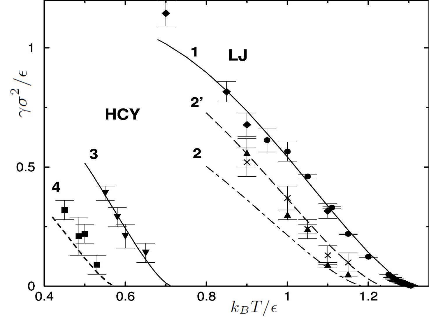
Figure 1: Reduced surface tension $\gamma\sigma^{2}/\epsilon$ as a function of the reduced temperature $k_{B}T/\epsilon$. Curves – theory, Eq. (32), points – numerical data. LJ-fluid: curve $1$, diamonds Mecke et al. (1997); Holcomb et al. (1993) and circles Potoff and Panagiotopoulos (2000). HCY-fluid: curves $2$, $2^{\prime}$, $3$ and $4$, stars and triangles up ($\lambda=1.8$ Gonzalez-Melchor et al. (2001)), triangles down ($\lambda=3.0$, Gonzalez-Melchor et al. (2001)) and squares ($\lambda=4.0$, Gonzalez-Melchor et al. (2001)). Critical parameters and $\sigma$, $\epsilon$, $\lambda$ are taken from Refs. Potoff and Panagiotopoulos (2000); Lomba and Almarza (1994); Duh and Mier-Y-Terán (1997); Gonzalez-Melchor et al. (2001), see the text for detail.

The theoretical predictions, Eq. (32), have been compared with the available data of numerical experiments for the Lennard-Jones (LJ) and hard-core Yukawa (HCY) fluids. For these systems the standard WCA partition (see e.g. Barker and Henderson (1976)) of the potential into attractive and repulsive parts has been applied Brilliantov (1998). The numerical data have been obtained for the LJ-fluid by means of molecular dynamics (MD) Mecke et al. (1997); Holcomb et al. (1993) and Monte Carlo Potoff and Panagiotopoulos (2000). For the HCY-fluid the MC and MD Gonzalez-Melchor et al. (2001) have been also applied. The critical parameters for the LJ-fluid were taken from Ref. Potoff and Panagiotopoulos (2000). For the HCY fluid we used the critical parameters from Ref. Lomba and Almarza (1994) for the curves $2$, $3$, $4$, and parameters from Ref. Duh and Mier-Y-Terán (1997) for the curve $2^{\prime}$. The values of $\sigma$ and $\epsilon$ for the LJ potential were taken from Ref. Potoff and Panagiotopoulos (2000) and $\sigma$, $\epsilon$, $\lambda$ for the HCY potential from Ref. Gonzalez-Melchor et al. (2001).

As follows from Fig. 1 our theory is in a good agreement with the numerical experiments. It is expected, however, that the agreement would be worse in the very close vicinity of the critical point, where the mean field theory loses its accuracy. The accuracy of numerical simulations also decreases in the vicinity of the critical point Brilliantov and Valleau (1998). Eq. (32) is quite sensitive to the critical parameters $\rho_{c}$, $T_{c}$. While these are known rather accurately for the LJ fluid, they are estimated with much larger uncertainty for the HCY fluid. This is demonstrated in Fig. 1, where two theoretical curves ($2$ and $2^{\prime}$) correspond to the same HCY fluid but with $\rho_{c}$, $T_{c}$, taken from different sources ($\rho_{c}$ and $T_{c}$ differ by about $4\%$).

IV Conclusion

We develop a theory of inhomogeneous simple fluids based on the microscopic one-body potential in fluid, which naturally emerges in the Hubbard-Schofield (HS) transformation. We demonstrate that the ”technical” field variable $\phi({\bf r})$, associated with the HS transformation, possesses a clear physical meaning. It gives the molecular potential at point ${\bf r}$ (in units of $k_{B}T$) from the attractive part of the inter-particle potential of molecules located in the vicinity of ${\bf r}$. Hence $\phi({\bf r})$ depends on both – on the particle density $\rho({\bf r})$ and on the attractive potential $v(r)$, being the convolution of $\rho({\bf r})$ and $v({\bf r})$. As the result, the microscopic field $\phi({\bf r})$ varies much more smoothly, even in the interface region than the local density $\rho({\bf r})$ itself. The smooth variation of $\phi({\bf r})$ guarantees the accuracy of the small gradient expansion, applied for the field-dependent Hamiltonian. Moreover, any additional smoothing procedure is not required. This makes the approach more simple and presumably more reliable. In contrast, the density functional theory, based on the local density, see e.g. Henderson (1992), exploits the smoothing of $\rho({\bf r})$ due to its sharp variation at the interface. The smoothing weight function is commonly chosen ad hoc, see e.g. Henderson (1992); Iatsevitch and Forstmann (1997, 2001).

Using the microscopic molecular field approach, which steams from the HS transformation we calculate the surface tension $\gamma$ for the liquid-vapor interface. Here we apply the mean-field approximation which considers only average molecular field and ignores the field fluctuations. We obtain an explicit analytical result for $\gamma$, which expresses this quantity in terms of temperature and density of the system and parameters of the inter-molecular potential. The theoretical predictions for the surface tension are in a good agreement with the results of numerical experiments. The mean-field approach loses however its accuracy in the very close vicinity to the critical point, where the near-critical fluctuations become important. The account of the critical fluctuation for $\gamma$ is straightforward and may be done applying the technique developed in Ref. Brézin and Feng (1984). Up to our knowledge, our study reports for the first time simple analytical expression for the surface tension that agrees well with the numerical experiments.

V Acknowledgements

NB gratefully acknowledges the financial support from the Russian Foundation for Basic Research under grant 18-29-19198. YB thanks Russian Foundation for Basic Research Grant No 18-29-06008 for financial support. JMR has been supported by MICINN of the Spanish Government under Grant No. PGC2018-098373-B-I00 and by the Catalan Goverment under the Grant 2017-SGR-884

References

- Amit (1978) D. Amit, Field theory, critical phenomena and the renormalization group (1978).
- Brézin (2010) E. Brézin, Introduction to Statistical Field Theory (Cambridge University Press, Cambridge, UK, 2010).
- Stratonovich (1957) R. L. Stratonovich, in Doklady Akademii Nauk (Russian Academy of Sciences, 1957), vol. 115, pp. 1097–1100.
- Kac (1959) M. Kac, The Physics of Fluids 2, 8 (1959).
- Hubbard (1959) J. Hubbard, Physical Review Letters 3, 77 (1959).
- Hubbard and Schofield (1972) J. Hubbard and P. Schofield, Physics Letters A 40, 245 (1972).
- Edwards (1965) S. F. Edwards, Proceedings of the Physical Society 85, 613 (1965).
- Edwards (1959) S. Edwards, Philosophical Magazine 4, 1171 (1959).
- Siegert (1960) A. Siegert, Physica 26 (1960).
- Caillol (2003) J.-M. Caillol, Molecular Physics 101, 1617 (2003).
- Caillol et al. (2005) J.-M. Caillol, O. Patsahan, and I. Mryglod, Journal of Physics: Condensed Matter 8, 665 (2005).
- Russier and Caillol (2010) V. Russier and J.-M. Caillol, Condensed Matter Physics 13, 23602 (2010).
- Brilliantov (1998) N. V. Brilliantov, Physical Review E 58, 2628 (1998).
- Ivanchenko and Lisyansky (1984) Y. M. Ivanchenko and A. A. Lisyansky, Teoreticheskaya i Matematicheskaya Fizika 58, 146 (1984).
- Budkov (2019a) Y. A. Budkov, Journal of Physics: Condensed Matter 32, 055101 (2019a).
- Budkov (2018) Y. A. Budkov, Journal of Physics: Condensed Matter 30, 344001 (2018).
- Budkov (2019b) Y. A. Budkov, Fluid Phase Equilibria 490, 133 (2019b).
- Zakharov and Loktionov (1999) A. Y. Zakharov and I. K. Loktionov, Theoretical and Mathematical Physics 119, 532 (1999).
- Adžić and Podgornik (2014) N. Adžić and R. Podgornik, The European Physical Journal E 37, 49 (2014).
- Efimov and Nogovitsin (1996) G. V. Efimov and E. A. Nogovitsin, Physica A: Statistical Mechanics and its Applications 234, 506 (1996).
- Baeurle (2002) S. A. Baeurle, Physical review letters 89, 080602 (2002).
- Netz (2001) R. R. Netz, The European Physical Journal E 5, 557 (2001).
- Lue (2006) L. Lue, Fluid phase equilibria 241, 236 (2006).
- Brézin and Feng (1984) E. Brézin and S. Feng, Physical Review B 29, 472 (1984).
- Brilliantov et al. (1998) N. V. Brilliantov, C. Bagnuls, and C. Bervillier, Physics Letters A 245, 274 (1998).
- Storer (1969) R. Storer, Australian Journal of Physics 22, 747 (1969).
- di Caprio and Badiali (2008) D. di Caprio and J. P. Badiali, J. Phys. A: Math. Theor. 41, 125401 (2008).
- Caillol et al. (2006) J.-M. Caillol, O. Patsahan, and I. Mryglod, Physica A: Statistical Mechanics and its Applications 368, 326 (2006).
- Parola and Reatto (1995) A. Parola and L. Reatto, Advances in Physics 44, 211 (1995).
- Frusawa (2018) H. Frusawa, Physical Review E 98, 052130 (2018).
- Stanley (1971) E. H. Stanley, Introduction to phase transitions and critical phenomena (1971).
- Landau and Lifshitz (2013) L. Landau and E. Lifshitz, Statistical Physics, Course of theoretical physics, v.5 (Elsevier, 2013).
- Kendon et al. (2001) V. M. Kendon, M. E. Cates, I. Pagonabarraga, J.-C. Desplat, and P. Bladon, Journal of Fluid Mechanics 440, 147 (2001).
- Gray and Gubbins (1984) C. Gray and K. Gubbins, Theory of Molecular Fluids: Vol. 1: Fundamentals (Clarendon Press, 1984).
- Barker and Henderson (1976) J. A. Barker and D. Henderson, Reviews of Modern Physics 48, 587 (1976).
- Widom (1965) B. Widom, The Journal of Chemical Physics 43, 3892 (1965).
- Mecke et al. (1997) M. Mecke, J. Winkelmann, and J. Fischer, The Journal of chemical physics 107, 9264 (1997).
- Holcomb et al. (1993) C. D. Holcomb, P. Clancy, and J. A. Zollweg, Molecular Physics 78, 437 (1993).
- Potoff and Panagiotopoulos (2000) J. J. Potoff and A. Z. Panagiotopoulos, The Journal of Chemical Physics 112, 6411 (2000).
- Gonzalez-Melchor et al. (2001) M. Gonzalez-Melchor, A. Trokhymchuk, and J. Alejandre, The Journal of Chemical Physics 115, 3862 (2001).
- Lomba and Almarza (1994) E. Lomba and N. G. Almarza, The Journal of chemical physics 100, 8367 (1994).
- Duh and Mier-Y-Terán (1997) D.-M. Duh and L. Mier-Y-Terán, Molecular Physics 90, 373 (1997).
- Henderson (1992) D. Henderson, Fundamentals of inhomogeneous fluids (CRC Press, 1992).
- Iatsevitch and Forstmann (1997) S. Iatsevitch and F. Forstmann, The Journal of chemical physics 107, 6925 (1997).
- Iatsevitch and Forstmann (2001) S. Iatsevitch and F. Forstmann, Journal of Physics: Condensed Matter 13, 4769 (2001).
- Trokhymchuk et al. (2017) A. Trokhymchuk, R. Melnyk, M. Holovko, and I. Nezbeda, Journal of Molecular Liquids 228, 194 (2017).
- Brilliantov and Valleau (1998) N. Brilliantov, and J. Valleau, The Journal of Chemical Physics 108, 1123-1130 (1998).