Statistical Verification of Autonomous Systems using Surrogate Models and Conformal Inference

Abstract

In this paper, we propose conformal inference based approach for statistical verification of CPS models. Cyber-physical systems (CPS) such as autonomous vehicles, avionic systems, and medical devices operate in highly uncertain environments. This uncertainty is typically modeled using a finite number of parameters or input signals. Given a system specification in Signal Temporal Logic (STL), we would like to verify that for all (infinite) values of the model parameters/input signals, the system satisfies its specification. Unfortunately, this problem is undecidable in general. Statistical model checking (SMC) offers a solution by providing guarantees on the correctness of CPS models by statistically reasoning on model simulations. We propose a new approach for statistical verification of CPS models for user-provided distribution on the model parameters. Our technique uses model simulations to learn surrogate models, and uses conformal inference to provide probabilistic guarantees on the satisfaction of a given STL property. Additionally, we can provide prediction intervals containing the the quantitative satisfaction values of the given STL property for any user-specified confidence level. We also propose a refinement procedure based on Gaussian Process (GP)-based surrogate models for obtaining fine-grained probabilistic guarantees over sub-regions in the parameter space. This in turn enables the CPS designer to choose assured validity domains in the parameter space for safety-critical applications. Finally, we demonstrate the efficacy of our technique on several CPS models.

1 Introduction

Cyber-physical systems (CPS) such as robotic ground and aerial vehicles, medical devices and industrial controllers are highly complex systems with nonlinear behaviors that operate in uncertain operating environments. As these systems are often safety-critical, it is desirable to obtain strong assurances on their safe operation. To achieve this goal, recent research has been focused on effective and sound verification algorithms [9, 19, 21, 38, 39, 10, 18, 45], and scalable best-effort approaches which lack explicit coverage guarantees [17, 28, 44]. However, factors like complexity and stochasticity of the operating environments, curse of dimensionality, the nonlinearity of dynamics pose a significant scalability challenge for verification procedures.

In this paper, we address the problem of analyzing the effects of uncertainty in the environment on the correctness of a given CPS model $\mathcal{M}$. We assume that the aleatoric uncertainty in the environment is modeled as discrete-time input signals to $\mathcal{M}$, where the signal value at each discrete time-step is assumed to come from some distribution. In addition, we also consider static parameters of $\mathcal{M}$, i.e. parameters that have a fixed value during a simulation run; examples include design parameters of $\mathcal{M}$ or parameters modeling variability in the sensor measurements and actuation errors. We can effectively lump these different parameters into a single multivariate random variable $\theta$ that takes values from some compact set $\Theta$, distributed according to some user-provided distribution $\mathcal{D}_{\Theta}$. For any single sample of $\theta$, we assume that the output trajectories of the model (denoted $\xi_{\theta}$) are deterministic, i.e. the model is free of any internal stochastic behavior. A distribution on the parameters induces a distribution on the output trajectories $\xi_{\theta}$ of the model.

The correctness of CPS models can be expressed using Signal Temporal Logic (STL) [26] formulas over the model trajectories. STL formulas are evaluated on trajectories, i.e. signals, and in this paper we assume signals to be finite sequences of time-value pairs. STL formulas have both Boolean and quantitative satisfaction semantics. The Boolean semantics are interpreted as follows: a signal $x$ either satisfies a formula $\varphi$ (denoted $x\models\varphi$) or it does not satisfy $\varphi$ (denoted $x\not\models\varphi$). The quantitative semantics are defined using a robustness value $\rho(\varphi,x)$ [8, 11]. Intuitively, $\rho(\varphi,x)$ gives a degree of satisfaction of $\varphi$ by $x$. In this paper we are interested in answering the following two questions:

1. For some user-provided threshold $\epsilon$, and $\theta\sim\mathcal{D}_{\Theta}$, is the probability of the model behavior satisfying a given STL property $\varphi$ more than $1-\epsilon$, or

   $$\theta\sim\mathcal{D}_{\Theta}\implies P(\mathcal{M}(\theta)\models\varphi)\geq 1-\epsilon$$ (1.1)

2. For some user-provided threshold $\epsilon$, and $\theta\sim\mathcal{D}_{\Theta}$, can we find an interval $[\ell,u]$ s.t. the probability that the robustness value of a model behavior $\mathcal{M}(\theta)$ w.r.t. a given STL property $\varphi$ lies in $[\ell,u]$ with probability greater than $1-\epsilon$? I.e.,

   $$\theta\sim\mathcal{D}_{\Theta}\implies P(\rho(\varphi,\mathcal{M}(\theta))\in[\ell,u])>1-\epsilon$$ (1.2)

Statistical model checking (SMC) [23, 2, 46, 45, 33, 36] approaches have been used in the past to establish assertions such as (1.1). The most popular SMC methods use statistical hypothesis testing procedures to check whether the hypothesis that (1.1) is true can be accepted with confidence exceeding user-specified thresholds $\alpha,\beta$ for respectively committing a type I error (i.e. accepting the hypothesis when it is not true), or a type II error( i.e. rejecting the hypothesis when it is true). SMC methods provide the user with conditions on the number of simulations required, $\alpha$, $\beta$ and $\epsilon$ in order to accept or reject the hypothesis (1.1).

Approach. To establish assertions such as (1.1) or (1.2), we present an approach based on conformal inference, a technique for giving confidence intervals with marginal coverage guarantees. A unique feature of our technique is that it does not make any assumptions on the user-provided distribution on the parameter space or the dynamics represented by the model.

We now give an overview of our approach as illustrated in Fig. 1. Given the parameterized system model $\mathcal{M}(\theta)$, a distribution $\mathcal{D}_{\Theta}$ over the space $\Theta$ of parameter values, and an STL property $\varphi$, we perform $N$ simulations model with these parameter values to obtain trajectories $\xi_{\theta}$. We then compute the robust satisfaction value $\rho(\varphi,\xi_{\theta})$ for each model trajectory.

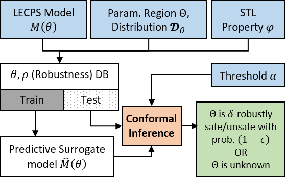
Figure 1: Overview of our approach.

Next, we consider some subset of the generated $\theta$ and corresponding $\rho(\varphi,\xi_{\theta})$ values and train a surrogate model $\hat{\mu}$ that takes in a parameter value $\theta$ and predicts a robustness value $\hat{\mu}(\theta)$ for all parameter values in the given region $\Theta$. Finally, we use the test set and a user-provided threshold $\epsilon$ as inputs to a combination of the conformal inference procedure with a global optimizer to compute a bound $d$ that guarantees that for all $\theta^{\prime}\in\Theta$,

$$P\left(\rho(\varphi,\xi_{\theta^{\prime}})\in\left[\hat{\mu}(\theta^{\prime})-d,\ \ \hat{\mu}(\theta^{\prime})+d\right]\right)\geq 1-\epsilon.$$

The above guarantee allows us to construct a confidence interval for the robustness of the property $\varphi$ over the given region $\Theta$. A strictly positive or strictly negative interval indicates that the $\Theta$ is respectively safe or unsafe. However, if the interval contains $0$, then the status of $\Theta$ remains unknown.

The above procedure naturally yields a refinement procedure which allows us to start with a larger region in the parameter space, and split it into smaller regions if the region is deemed unknown. In a smaller region, the accuracy of the surrogate model improves (due to more data in a smaller region), and hence previously inconclusive regions can be resolved as safe/unsafe. A naïve version of this splitting algorithm faces the curse of dimensionality – if the parameter space is high-dimensional then the branch-and-bound procedure ends up creating too many branches which can make the procedure intractable. In order to address this shortcoming, we investigate a procedure that uses a Gaussian Process based surrogate model combined with Bayesian optimization to split the parameter regions in a smart manner. Gaussian processes explicitly encode sample uncertainty, which allows us to perform splitting that adapts to the robustness surface, thereby reducing the number of regions that the algorithm examines.

Our method can scale to CPS models encoding complex dynamics and large state spaces, as well as reasonably large parameter spaces. The results of our method can be used to characterize safe operating regions in the parameter space, and to build (probabilistic) safety assurance cases. With respect to analysis times, our method compares favorably with approaches based on statistical model checking (SMC). However, unlike SMC and PAC based methods the provided guarantee is not a function of the number of samples. In fact, our method can potentially provide the needed level of probabilistic guarantees with any number of samples. This is because we build a surrogate model from samples; if the surrogate model is of poor accuracy due to a limited number of samples, conformal inference will predict a wider interval of robustness values with the same level of guarantees $1-\alpha$, while for a more accurate model, the robustness interval will be narrower. Thus, conformal inference allows a trade-off between sample complexity and the tightness of the guarantee independent of the level of the guarantee itself.

The main contributions of this paper are:

1. A technique based on surrogate models to approximate the robustness of a given specification learned using off-the-shelf regression techniques.

2. A new technique for generating prediction intervals for the robustness of a specification with user-specified probabilistic thresholds.

3. Algorithms to partition the parameter space of a model into safe, unsafe and unknown regions based on conformal inference on the surrogate models.

4. Experimental validation on CPS models demonstrating the real-world applicability of our methods.

The rest of the paper is organized as follows. Section 2 provides the background and notation. Section 3 explains how we use conformal inference for providing probabilistic guarantees on satisfaction/violation of a given STL property over a region in the parameter space. Section 4 presents our algorithm for refining parameter spaces using Gaussian Processes. Finally, Section 5, illustrates our approach using several case studies and Section 6 presents our conclusions.

2 Preliminaries

Definition 1 (Signals, Black-box Models)

We define a signal or a trajectory $\xi$ as a function from a set ${\mathsf{dom}}=[0,T]$ for some $T\in\mathbb{R}^{\geq 0}$ to a compact set of values $\mathcal{X}$. The signal value at time $t$ is denoted as $\xi(t)$. A parameter space $\Theta$ is some compact subset of $\mathbb{R}^{k}$. A model $\mathcal{M}$ is a function that maps a parameter value $\theta\in\Theta$ to an output signal $\xi_{\theta}$.

We note that the above definition permits parameterized input signals for the model. We can define such signals using a function known as a signal generator that maps specific parameter values to signals. For example, a piecewise linear signal containing $k$ linear segments can be described using $k+1$ parameters, $k$ corresponding to the starting point for each segment and $1$ for the end-point of the final segment.

We assume that $\theta\in\Theta$ is a random variable that follows a (truncated) distribution $\mathcal{D}_{\theta}$ with probability density function (PDF) $f(\theta)$ and $\forall\theta\notin\Theta,f(\theta)=0$. If we only wish to draw samples from a subset $S\subseteq\Theta$ (by dropping samples from $\Theta\setminus S$), the corresponding distribution of the samples is denoted by $\mathcal{D}_{\theta}\mathrel{\downarrow}S$ and follows the PDF shown below.

$$f^{\prime}(\theta)=\left\{\begin{array}[]{ll}\frac{f(\theta)}{\int_{\tau\in S}f(\tau)d\tau}&\mbox{if~{}}\theta\in S\\ 0&\mbox{otherwise}.\end{array}\right.$$ (2.1)

Instead of closed form descriptions of the generator for $\xi_{\theta}$ (e.g. differential or difference equations), we assume that there is a simulator that can generate signals compatible with the semantics of the model $\mathcal{M}$.

Definition 2

A simulator for a (deterministic) set $\Xi$ of trajectories is a function (or a program) ${\mathsf{sim}}$ that takes as input a parameter $\theta\in\Theta$, and a finite sequence of time points $t_{0},\ldots,t_{k}$, and returns the signal ($t_{0},{\mathsf{sim}}(\theta,t_{0})$, $\ldots$, $t_{k},{\mathsf{sim}}(\theta,t_{k})$), where for each $i\in\{0,\ldots,k\}$, ${\mathsf{sim}}(\theta,t_{i})=\xi_{\theta}(t_{i})$.

In rest of the paper, unless otherwise specified, we ignore the distinction between the signals ${\mathsf{sim}}(\theta,\cdot)$ and $\xi_{\theta}$.

2.1 Signal Temporal Logic

Signal Temporal Logic [26] is a popular formalism that has been used widely used to express safety specifications for many CPS applications. STL formulas are defined over signal predicates of the form $f(\xi)\geq c$ or $f(\xi)\leq c$, where $\xi$ is a signal and $f:\mathbb{R}^{n}\rightarrow\mathbb{R}$ is a real-valued function and $c\in\mathbb{R}$. STL formulas are written using the grammar shown in Eq. (2.2). Here, we assume that $I=[a,b]$, where $a,b\in\mathbb{R}^{\geq 0},a\leq b$, and $\sim\in\{\leq,\geq\}$.

$$\varphi,\psi:=\mathit{true}\mid f(\xi)\sim c\mid\neg\varphi\mid\varphi\wedge\psi\mid\varphi\vee\psi\mid\mathbf{F}_{I}\varphi\mid\mathbf{G}_{I}\varphi\mid\varphi~{}\mathbf{U}_{I}~{}\psi$$ (2.2)

In the above syntax, $\mathbf{F}$ (eventually), $\mathbf{G}$ (always), and $\mathbf{U}$ (until) are temporal operators. Given $t\in\mathbb{R}^{\geq 0}$ and $I=[a,b]$, we use $t+I$ to denote $[t+a,t+b]$. Given a signal $\xi$ and a time $t$, we use $(\xi,t)\models\varphi$ to denote that $\xi$ satisfies $\varphi$ at time $t$, and $\xi\models\varphi$ as short-hand for $(\xi,0)\models\varphi$. The Boolean satisfaction semantics of an STL formula can be recursively in terms of the satisfaction of its subformulas over the a signal. For $\sim\in\{\leq,\geq\}$, $\xi$: $(\xi,t)\models f(\xi)\sim c$ if $f(\xi(t))\sim c$ is true. The semantics of the Boolean operators for negation ($\neg$), conjunction ($\wedge$) and disjunction ($\vee$) can be obtained in the usual fashion by applying the operator to the Boolean satisfaction of its operand(s). The value of $(\xi,t)\models\mathbf{F}_{I}\varphi$ is true iff $\exists t^{\prime}\in t+I$ s.t. $(\xi,t^{\prime})\models\varphi$, while $(\xi,t)\models\mathbf{G}_{I}\varphi$ iff $\forall t^{\prime}\in t+I$, $(\xi,t^{\prime})\models\varphi$. The formula $\varphi\mathbf{U}_{I}\psi$ is satisfied at time $t$ if there exists a time $t^{\prime}$ s.t. $\psi$ is true, and for all $t^{\prime\prime}\in[t,t^{\prime})$, $\varphi$ is true.

STL is also equipped with quantitative semantics that define the robust satisfaction value or robustness – a function mapping a formula $\varphi$ and the signal $\xi$ to a real number [11, 8]. Informally, robustness can be viewed as a degree of satisfaction of an STL formula $\varphi$. While many competing definitions for robust satisfaction value exist [3, 31, 20], we use the original definitions [8] in this paper.

Definition 3

The robustness value is a function $\rho$ mapping $\varphi$, the trajectory $\xi$, and a time $t\in\xi.{\mathsf{dom}}$ as follows:

$$\small\begin{array}[]{rcl}\rho(f(\xi)\geq c,\xi,t)&=&f(\xi(t))-c\\ \rho(\neg\varphi,\xi,t)&=&-\rho(\varphi,\xi,t)\\ \rho(\varphi\wedge\psi,\xi,t)&=&\min(\rho(\varphi,\xi,t),\rho(\psi,\xi,t))\\ \rho(\varphi~{}\mathbf{U}_{I}~{}\psi)&=&\sup\limits_{t_{1}\in t+I}\min(\rho(\psi,\xi,t_{1}),\inf\limits_{t_{2}\in[t,t_{1})}\rho(\varphi,\xi,t_{2}))\\ \end{array}$$

The robustness values for other Boolean and temporal operators can be derived from the above definition; for example, $\mathbf{G}_{I}\varphi$ and $\mathbf{F}_{I}\varphi$ are a special case of the semantics for until ($\mathbf{U}_{I}$) respectively evaluating to the minimum and maximum of the robustness of $\varphi$ over the interval $I$.

Example 1

Consider the time-reversed van Der Pol oscillator specified as $\dot{x_{1}}=-x_{2}$, $\dot{x_{2}}=4(x_{1}^{2}-1)x_{2}+x_{1}$. Figure 2 illustrates the satisfaction (indicated in blue) and violation (indicated in red) of two example specifications by $x_{1}(t)$: (a) $\varphi_{1}$ specifies that for any time $t\in[0,10]$, the value of the trajectory $x(t)$ should be less than $0.5$ and (b) $\varphi_{2}$ specifies that from some time within the first $2$ time units, $x(t)$ settles in the region $[-0.3,0.3]$ for $8$ time units.

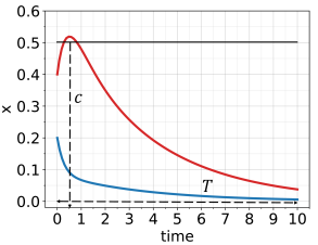
(a) $\varphi_{1}=\mathbf{G}_{[0,10]}(x(t)<0.5)$

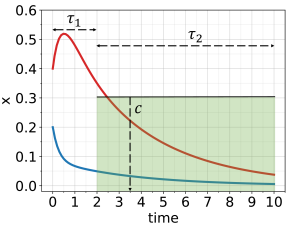
(b) $\varphi_{2}=\mathbf{F}_{[0,2]}\mathbf{G}_{[0,8]}(\|x(t)\|<0.3)$

Figure 2: Example of trajectories satisfying (blue) and violating (red) the STL formulas.

2.2 Learning Surrogate Models

In this section we discuss learning of surrogate models for a given black-box model $\mathcal{M}$. A surrogate model is essentially a quantitative abstraction of the original black-box model. Quantitative abstractions have been explored in the theory of weighted transition systems (WTS) [6]. A WTS is a transition system where every transition is associated with weights, and a quantitative property of the WTS maps sequences of states of the WTS to a real number computed using some arithmetic operations on the weights. Quantitative abstractions focus on sound proofs for quantitative properties. We observe that we can view the robustness of an STL property as a quantitative property evaluated on the system trajectory. We introduce two new notions of quantitative abstractions defined on the trajectories of a system.

Definition 4 ($\delta$-surrogate model)

Let $\xi_{\theta}$ be the trajectory obtained by simulating the $\mathcal{M}$ with the parameter $\theta$, where $\theta\in\Theta$. Let $\gamma$ be a quantitative property on $\xi_{\theta}$, i.e. $\gamma$ maps $\xi_{\theta}$ to a real number. We say that a model $\hat{\mu}$ that maps $\theta$ to a real number is an $\delta$-distance-preserving quantitative abstraction or an $\delta$-surrogate model of $\mathcal{M}$ and $\gamma$ if

$$\exists\delta:\forall\theta\in\Theta:|\gamma(\xi_{\theta})-\hat{\mu}(\theta)|\leq\delta$$ (2.3)

Essentially, the $\delta$-surrogate model guarantees that the value of the quantitative property $\gamma$ evaluated on $\xi_{\theta}$ (obtained from the original model $\mathcal{M}$) is no more than $\delta$ away from the value that it predicts. The idea is that the $\delta$-surrogate model could be systematically derived from the original model, and could be significantly simpler than the original model making it amenable to formal analysis. For example, if we have an $\delta$-surrogate model, then we can prove that a given property holds by systematically sampling the parameter space $\Theta$.

In general, such models could be hard to obtain; hence, we propose a probabilistic relaxation known as the $(\delta,\epsilon)$-probabilistic surrogate model, where condition (2.3) is replaced by (2.4).

Definition 5 ($(\delta,\epsilon)$-probabilistic surrogate model)

Given a model $\mathcal{M}$, a quantitative property $\gamma$, and a user-specified bound $\epsilon\in[0,1)$, we say that $\hat{\mu}$ is a $(\delta,\epsilon)$-probabilistic surrogate model if:

$$\exists\delta\in\mathbb{R},\epsilon\in[0,1):P\left(|\gamma(\xi_{\theta})-\hat{\mu}(\theta)|\leq\delta\mid\theta\sim\mathcal{D}_{\theta}\right)\geq 1-\epsilon$$ (2.4)

We now explain how we can obtain $(\delta,\epsilon)$-probabilistic surrogate models for an arbitrary quantitative property $\gamma$. The basic idea is to use statistical learning techniques: we sample $\Theta$ in accordance with the distribution $\mathcal{D}_{\theta}$ to obtain a finite set of parameter values $\widehat{\Theta}$. For each $\theta_{i}\in\widehat{\Theta}$, we simulate the model to obtain $\xi_{\theta_{i}}$ and compute $\gamma(\xi_{\theta_{i}})$. We then compute the surrogate model $\hat{\mu}$ using parametric regression models (e.g. linear, polynomial functions) or nonparametric regression methods (e.g. neural networks and Gaussian Processes) [14, 4, 30]. We now briefly review some of these regression methods, and in Section 3 explain how we can obtain $\delta$ values for a user-provided bound $\epsilon$.

Polynomial Regression. Polynomial regression assumes a polynomial relationship between independent variables $X$ and the dependent variable $Y$. It aims to fit a polynomial curve to the input and output data in a way that minimizes a suitable loss function. A commonly used loss function is the least square error (or the sum of squares of residuals). Typically, a polynomial regression requires the user to specify the degree of the polynomial to use. Polynomial regression generally has high tolerance to the function’s curvature level, but has high sensitivity to the outliers. In our experiments, we restrict the polynomial degree to 2.

Neural Network Regression. Neural networks [5] offer a high degree of flexibility for regressing arbitrary nonlinear functions. While there are many different NN architectures, we use a simple multi-layer perceptron model with a stochastic gradient-based optimizer. This model simply updates its parameters based on iterative steps along the partial derivatives of the loss function.

Gaussian Process based Regression Model [30]. A Gaussian Process (GP) is a stochastic process, i.e., it is a collection of random variables $W_{\theta}$ indexed by $\theta$, where $\theta$ ranges over some discrete or dense set. The key property of GP is that any finite sub-collection of these random variables has a multi-variate Gaussian distribution. GP models are popular as non-parametric regression methods used for approximating arbitrary continuous functions with the appropriate kernel functions. A GP can be used to express a prior distribution on the space of functions, e.g. from a domain $\mathbb{R}^{n}$ to $\mathbb{R}$. Let $F:\mathbb{R}^{n}\to\mathbb{R}$ be a random function. Then, we say that $F$ is a centered Gaussian process with kernel $k$, if for every $(x_{1},\ldots,x_{n})\in\mathbb{R}^{n}$, there exists a positive semi-definite matrix $\Sigma$ such that $[F(x_{1}),\ldots,F(x_{n})]\sim(0,\Sigma)$. The $(i,j)^{th}$ entry of $\Sigma$, i.e. $\Sigma_{ij}=k(x_{i},x_{j})$ for some kernel function $k$. The matrix $\Sigma$ is called the covariance matrix, and the function $k$ measures the joint variability of $x_{i}$ and $x_{j}$. There are several kernel functions that are popular in literature: the squared exponential kernel, the 5/2 Matérn kernel, etc. In our experiments, we use a sum kernel function that is the addition of a dot product kernel and a white noise kernel (explained in Section 4).

3 Conformal Inference

Conformal inference [24, 25] is a framework to quantify the accuracy of predictions in a regression framework [41]. It can provide guarantees using a finite number of samples, without making assumptions on the distribution of data used for regression or the technique used for regression. We explain the basic idea of conformal inference, and then explain how we adapt it to our problem setting.

3.1 Conformal Inference Recap

Consider i.i.d. regression data $Z_{1},\cdots,Z_{m}$ drawn from an arbitrary joint $\mathcal{D}_{XY}$, where each $Z_{i}=(X_{i},Y_{i})$ is a random variable in $\mathbb{R}^{n}\times\mathbb{R}$, consisting of $n$-dimensional feature vectors $X_{i}$ and a response variable $Y_{i}$. Suppose we fit a surrogate model to the data, and we now wish to use this model to predict a new response $Y_{m+1}$ for a new feature value $X_{m+1}$, with no assumptions on $\mathcal{D}_{XY}$. Formally, given a positive value $\alpha\in(0,1)$, conformal inference constructs a prediction band $C\subseteq\mathbb{R}^{n}\times\mathbb{R}$ based on $Z_{1},\cdots,Z_{n}$ with property (3.1).

$$P(Y_{m+1}\in C(X_{m+1}))\geq 1-\alpha.$$ (3.1)

Here, the probability is over $m+1$ i.i.d. draws $Z_{1},\cdots,Z_{m+1}\sim\mathcal{D}_{XY}$, and for a point $x\in\mathbb{R}^{n}$ we denote $C(x)=\{y\in\mathbb{R}:(x,y)\in C\}$. The parameter $\alpha$ is called the miscoverage level and $1-\alpha$ is called the probability threshold. Let

$$\mu(x)=\mathbb{E}(Y\ |\ X=x),x\in\mathbb{R}^{n}$$

denote the regression function, where $\mathbb{E}(W)$ denotes the expected value of the random variable $W$. The regression problem is to estimate such a conditional mean of the test response $Y_{m+1}$ given the test feature $X_{m+1}=x$. Common regression methods use a regression model $g(x,\eta)$ and minimize the sum of squared residuals of such model on the $m$ training regression data $Z_{1},\cdots,Z_{m}$, where $\eta$ are the parameters of the regression model. An estimator for $\mu$ is given by $\hat{\mu}(x)=g(x,\hat{\eta})$, where

$$\hat{\eta}=\displaystyle\operatorname*{arg\,min}_{\eta}\frac{1}{m}\sum_{i=1}^{m}\left(Y_{i}-g(X_{i},\eta)\right)^{2}+\mathcal{R}(\eta)$$

and $\mathcal{R}(\eta)$ is a regularizer. In [24], the authors provide a technique called split conformal prediction that we use to construct prediction intervals that satisfy the finite-sample guarantees as in Equation (3.1). The procedure is described in Algorithm 1 as a function $\mathtt{ConfInt}$ which takes as input the i.i.d. training data $\{(X_{i},Y_{i})\}_{i=1}^{m}$, miscoverage level $\alpha$ and any regression algorithm $\mathtt{Reg}$. Algorithm 1 begins by splitting the training data into two equal-sized disjoint subsets. Then a regression estimator $\hat{\mu}$ is fit to the training set $\{(X_{i},Y_{i})\}:i\in\mathcal{I}_{1})$ using the regression algorithm $\mathtt{Reg}$ (Line 1). Then the algorithm computes the absolute residuals $R_{i}$s on the test set $\{(X_{i},Y_{i})\}:i\in\mathcal{I}_{2})$ (Line 1). For the desired probability threshold $\alpha\in[0,1)$, the algorithm sorts the residuals in ascending order $\{R_{i}:i\in\mathcal{I}_{2}\}$ and finds the residual at the position given by the expression: $\left\lceil(n/2+1)(1-\alpha)\right\rceil$. This residual is used as the confidence range $d$. In [24], the authors prove that the prediction interval at a new point $X_{m+1}$ is given by such $\hat{\mu}$ and $d$ that Theorem 3.1 is valid.

input : Data $\{(X_{i},Y_{i})\}_{i=1}^{m}$, miscoverage level $\alpha$, regression algorithm $\mathtt{Reg}$

output : Regression estimator $\hat{\mu}$, confidence range $d$

1 Randomly split $\{1,\cdots,n\}$ into two equal-sized subsets $\mathcal{I}_{1},\mathcal{I}_{2}$;

2 $\hat{\mu}=\mathtt{Reg}((X_{i},Y_{i}):i\in\mathcal{I}_{1})$  ;

3 $R_{i}=|Y_{i}-\hat{\mu}(X_{i})|,i\in\mathcal{I}_{2}$ ;

4 $d=$ the $k$th smallest value in $\{R_{i}:i\in\mathcal{I}_{2}\}$, where $k=\lceil(n/2+1)(1-\alpha)\rceil$ ;

return $\hat{\mu},d$

Algorithm 1 Conformal regression algorithm $\mathtt{ConfInt}(\{(X_{i},Y_{i})\}_{i=1}^{m},\alpha,\mathtt{Reg})$

Theorem 3.1 (Theorem 2.1 in [24])

If $(X_{i},Y_{i}),i=1,\cdots,m$ are i.i.d., then for an new i.i.d. draw $(X_{m+1},Y_{m+1})$, using $\hat{\mu}$ and $d$ constructed in Algorithm 1, we have that $P(Y_{m+1}\in[\hat{\mu}(X_{m+1})-d,\hat{\mu}(X_{m+1})+d])\geq 1-\alpha.$ Moreover, if we additionally assume that the residuals $\{R_{i}:i\in\mathcal{I}_{0}\}$ have a continuous joint distribution, then $P(Y_{m+1}\in[\hat{\mu}(X_{m+1})-d,\hat{\mu}(X_{m+1})+d])\leq 1-\alpha+\frac{2}{m+2}.$ $\square$

Generally speaking, as we improve our surrogate model $\hat{\mu}$ of the underlying regression function $\mu$, the resulting conformal prediction interval decreases in length. Intuitively, this happens because a more accurate $\hat{\mu}$ leads to smaller residuals (or $\epsilon$ in Section 2.2), and conformal intervals are essentially defined by the quantiles of the (augmented) residual distribution. Note that Theorem 3.1 asserts marginal coverage guarantees, which should be distinguished with the conditional coverage guarantee $P(Y_{m+1}\in C(x)\ |\ X_{m+1}=x)\geq 1-\alpha$ for all $x\in\mathbb{R}^{n}$. The latter one is a much stronger property and hard to be achieved without assumptions on $\mathcal{D}_{XY}$.

3.2 Computing $(\delta,\epsilon)$-probabilistic surrogate models

We assume that the parameter value $\theta$ and $\rho(\varphi,\xi_{\theta})$ follow a joint (unknown) distribution $\mathcal{D}_{\theta,\rho(\varphi)}$ that we wish to empirically estimate. As indicated in Section 2.2, the first step to learning a $(\delta,\epsilon)$-probabilistic surrogate model is based on sampling $\mathcal{D}_{\theta,\rho(\varphi)}$ and applying regression methods. We draw $m$ i.i.d samples $\widehat{\Theta}=\{\theta_{1},\cdots,\theta_{m}\}$ from $\mathcal{D}_{\theta}$ and compute the robustness values $\rho_{i}=\rho(\varphi,\xi_{\theta_{i}})$ for each model trajectory corresponding to the parameter $\theta_{i}$. Lemma 1 follows from Theorem 3.1.

Lemma 1

Let $(\hat{\mu},d)=\mathtt{ConfInt}(\{\theta_{i},\rho_{i}\},\epsilon,\mathtt{Reg})$, where $\mathtt{ConfInt}$ is as defined in Algorithm 1, $1-\epsilon$ is a user-provided probability threshold, $\mathtt{Reg}$ is some regression algorithm, and $d\in\mathbb{R}$, then $\hat{\mu}$ is a $(d,\epsilon)$-probabilistic surrogate model.

We now show how we can use $(\delta,\epsilon)$-probabilistic surrogate models to perform statistical verification. Theorem 3.2 gives shows that the confidence range returned by the conformal inference procedure can be extended over the entire parameter space.

Theorem 3.2

Let

1. $(\theta_{i},\rho_{i}),i=1,\cdots,m$ be i.i.d. samples drawn from the joint distribution $\mathcal{D}_{\theta,\rho(\varphi)}$ of $\theta\in\Theta$ and $\rho(\varphi,\xi_{\theta})$,

2. $\mathtt{Reg}$ be a regression algorithm,

3. $1-\epsilon$ be a user-provided probability threshold,

4. $(\hat{\mu},d)=\mathtt{ConfInt}(\{\theta_{i},\rho_{i}\},\epsilon,\mathtt{Reg})$, i.e. $\hat{\mu}$ is the surrogate model and $d$ is the confidence range returned by Algorithm 1,

5. $v^{*}_{\max}=\max_{\theta\in\Theta}\hat{\mu}(\theta)$, and, $v^{*}_{\min}=\min_{\theta\in\Theta}$.

Then,

$$P\left(\rho(\varphi,\xi_{\theta})\in[v^{*}_{\min}-d,v^{*}_{\max}+d]\mid\theta\sim\mathcal{D}_{\theta}\right)\geq 1-\epsilon$$ (3.2)

Proof

From Theorem 3.1, we know that any new i.i.d. sample $(\theta^{\prime},\rho(\varphi,\xi_{\theta^{\prime}}))$ from $\mathcal{D}_{\theta,\rho(\varphi)}$ satisfies:

$$P(\rho(\varphi,\xi_{\theta^{\prime}})\in[\hat{\mu}(\theta^{\prime})-d,\hat{\mu}(\theta^{\prime})+d])\geq 1-\epsilon.$$ (3.3)

By definition, $v^{*}_{\min}\leq\hat{\mu}(\theta^{\prime})\leq v^{*}_{\max}$. Combining this with Eq. (3.3), we get the desired result.

Theorem 3.1 requires us to obtain the minimum/maximum values of the surrogate model over a given region in the parameter space. If $\hat{\mu}(\theta)$ is a non-convex function and the chosen optimization algorithm cannot compute the perfect optimal value $v^{*}_{\min}$ or $v^{*}_{\max}$, but can only give conservative estimates of the optimal value, we can update the predicted interval in Theorem 3.2 as follows.

Corollary 1

Let $v_{\min}$ and $v_{\max}$ be respectively under- and over-approximations of $v^{*}_{\min}$ and $v^{*}_{\max}$, then

$$P\left(\rho(\varphi,\xi_{\theta})\in[v_{\min}-d,v_{\min}+d]\mid\theta\sim\mathcal{D}_{\theta}\right)\geq 1-\epsilon$$ (3.4)

The bounds $v_{\min}$ and $v_{\max}$ in Corollary 1 can be computed using global optimization solvers, SMT sovlers, or range analysis tools for neural networks [39, 10], based on the kind of regression model used.

We can use the bounds obtained in Theorem 3.2 (similarly those with Corollary 1) to derive probabilistic bounds on the Boolean satisfaction of a given STL property $\varphi$, as expressed in Theorem 3.3.

Theorem 3.3

If $v^{*}_{\min}-d>0$, then $P_{\mathcal{D}_{\theta}}(\xi_{\theta}\models\varphi\mid\theta\in\Theta)\geq 1-\epsilon$. If $v^{*}_{\max}+d<0$ then $P_{\mathcal{D}_{\theta}}(\xi_{\theta}\not\models\varphi\mid\theta\in\Theta)\geq 1-\epsilon$.

Proof

From [11], we know that $\rho(\varphi,\xi_{\theta})>0\implies\xi_{\theta}\models\varphi$. Thus, if the lower bound of the prediction interval in Theorem 3.2 is positive, then $\xi_{\theta}\models\varphi$. The second case follows by a similar argument.

If the first statement in the above theorem holds, we say that $\Theta$ safe, if the second statement holds, we say that $\Theta$ is unsafe, and if neither statement holds (i.e. the predicted interval contains $0$), then we say that $\Theta$ is unknown. While Theorem 3.3 allows us a way to identify whether a region in the parameter space is is safe (or unsafe), unfortunately there are two challenges: (1) the function mapping $\theta$ to $\rho(\varphi,\overline{\mathsf{sim}}(\theta))$ is a highly nonlinear function in general, and a priori choice for a regression algorithm $\mathtt{Reg}$ that fits this function with small residual values may be difficult, (2) if there is large variation in the value of the regression function over $\Theta$, it is likely that the conformal interval contains $0$, thereby marking $\Theta$ as unknown. To circumvent this issue, one solution is to split the parameter space $\Theta$ into smaller regions where it may be possible to get narrow conformal intervals at the same level of probability threshold. We present a naïve algorithm based on parameter-space partitioning next.

3.3 Naïve Parameter Space Partitioning

We now present an algorithm that uses Theorem 3.2 (or Corollary 1) to provide probabilistic guarantee by recursively splitting the parameter space $\Theta$ into smaller regions such that each region can be labeled as safe, unsafe or unknown. The basic idea of this algorithm is to compute the conformal interval using Theorem 3.2 and then check if $v^{*}_{\min}-d<0$ and $v^{*}_{\max}+d>0$. If yes, we need to partition the region. After partitioning the region, we have to repeat the process of computing the conformal interval for each of the sub-regions. Note that the probability in Theorem 3.2 (and Theorem 3.1 ) is marginal, being taken over all the i.i.d. samples $\{\theta_{i},\rho_{i}\}$ from $\mathcal{D}_{\theta,\rho(\varphi)}$. Therefore, when we work on each subset $S\subseteq\Theta$ after the partitions, we will have to restrict $\theta$ to be in $S$ (according to Equation (2.1)) to ensure that the Theorem 3.2 is valid. We abuse the notation and denote the joint distribution $\mathcal{D}_{\theta,\rho(\varphi)}$ when $\theta$ is restricted to be sampled from $S\subseteq\Theta$ by $\mathcal{D}_{\theta,\rho(\varphi)}\mathrel{\downarrow}S$.

input : Parameter space $\Theta$ and corresponding distribution $\mathcal{D}_{\theta}$, simulator ${\mathsf{sim}}$ and interpolation method to provide $\overline{\mathsf{sim}}$, miscoverage level $\alpha$, regression algorithm $\mathtt{Reg}$, an STL formula $\varphi$, a vector $\Delta$

output : Parameter set $\Theta^{+}$ that lead to satisfaction of $\varphi$, $\Theta^{-}$ that lead to violation of $\varphi$, and the rest parameter set $\Theta^{U}$ that is undecided

1 $\Theta^{+},\Theta^{-},\Theta^{U}\leftarrow\emptyset$, $\Theta^{r}\leftarrow\{\Theta\}$;

2 while  $\Theta^{r}\neq\emptyset$  do

3       $S\leftarrow\mathtt{Pop}(\Theta^{r})$ ;

4       $\theta_{1},\cdots,\theta_{m}\leftarrow\mathtt{IID\_Sample}(\mathcal{D}_{\theta}\mathrel{\downarrow}S)$ ;

5       for $i=1,\cdots,m$ do

6             $\rho_{i}\leftarrow\rho(\varphi,\xi_{\theta_{i}})$ ;

7            

8      $\hat{\mu},d\leftarrow\mathtt{ConfInt}(\{(\theta_{i},\rho_{i})\}_{i=1}^{m},\alpha,\mathtt{Reg})$;

9       $v_{\max}\leftarrow\max_{\theta\in S}\hat{\mu}(\theta)$, $v_{\min}\leftarrow\min_{\theta\in S}\hat{\mu}(\theta)$;

10       if $v_{\min}-d\geq 0$ then

11             $\Theta^{+}\leftarrow\Theta^{+}\cup(S,[v_{\min}-d,v_{\max}+d])$ ;

12            

13       else if $v_{\max}+d\leq 0$ then

14             $\Theta^{-}\leftarrow\Theta^{-}\cup(S,[v_{\min}-d,v_{\max}+d])$ ;

15            

16       else if $\mathtt{Diameters}(S)<\Delta\mathtt{Diameters}(\Theta)$ then

17             $\Theta^{U}\leftarrow\Theta^{U}\cup(S,[v_{\min}-d,v_{\max}+d])$ ;

18            

19       else

20             $\Theta^{r}.\mathtt{Push}(\mathtt{Partition}(S,\mathtt{Reg}))$ ;

21            

22 return $\Theta^{+},\Theta^{-},\Theta^{U}$;

Algorithm 2 Parameter space partition with respect to STL formulas using conformal regression.

Algorithm 2 searches over the parameter space $\Theta$ and partitions it to sets $\Theta^{+}$, $\Theta^{-}$, and $\Theta^{U}$, along with the prediction intervals for the robustness values in each set. We first check if the robustness value is strictly positive or negative and accordingly add the region being inspected $S$ into $\Theta^{+}$ or $\Theta^{-}$ (Lines 2 and 2). When Algorithm 2 cannot decide whether $S$ belongs to $\Theta^{+}$ or $\Theta^{-}$ the interval contains $0$, we first check if for all $n$, the diameter of $S$ along the $n^{th}$ parameter dimension less than the fraction $\Delta_{n}\mathtt{Diameters}(\Theta)_{n}$. We assume that the vector $\Delta$ is provided by the user. If yes, the region is marked as unknown. Otherwise, we partition $S$ into a number of subregions, that are then added to a worklist of regions (Line 2). In our implementation, in order to keep the number of subsets to be explored bounded, we randomly pick a dimension in the parameter space, and split the parameter space into two equal subsets along that dimension. Note that the partitioning can be accelerated by using parallel computation, but we leave that for future exploration. For each subset $S$, Algorithm 2 additionally gives the corresponding prediction interval, which indicates how good (or bad) the trajectories satisfy (or violate) $\varphi$.

Theorem 3.4

In Algorithm 1, $P(\xi_{\theta}\models\varphi\mid\theta\sim\mathcal{D}_{\theta,\rho(\varphi)}\mathrel{\downarrow}\bigcup S\in\Theta^{+})\geq 1-\epsilon,$, and $P(\xi_{\theta}\not\models\varphi\mid\theta\sim\mathcal{D}_{\theta,\rho(\varphi)}\mathrel{\downarrow}\bigcup S\in\Theta^{-})\geq 1-\epsilon.$

Theorem 3.4 directly follows from Theorems 3.2 and 3.3 and the total probability theorem.

4 Gaussian Processes for Refinement

A drawback of Algorithm 2 is that the naïve splitting procedure is not scalable in high dimensions, and may have poor performance if the safe/unsafe regions have arbitrary shapes. In this section, we instead suggest the use of Gaussian Processes (GP) coupled with Bayesian updates to intelligently partition regions. Recall from Section 2, for each parameter value $\theta$, the GP model allows representing the mean $\mu(\theta)$ and $\sigma^{2}(\theta)$ in terms of samples already explored in the parameter space. In a GP model, at sampled parameter values, the variance is zero, but at points that are away from the sampled values, the variance could be high. We now give the symbolic expressions for the mean and variance of a GP model in terms of a kernel function $k(\theta,\theta)$. For ease of exposition let $\hat{\Theta}$ denote the vector of parameter values already sampled. Then, Let $Y$ denote the vector of robustness values for parameter values in $\hat{\Theta}$. Then, from [30], Chapter 2, we have:

$$\mu(\theta) = k(\theta,\hat{\Theta})^{\top}\,k(\hat{\Theta},\hat{\Theta})^{-1}\,Y$$ (4.1)

$$\Sigma(\theta) = k(\theta,\theta)-k(\theta,\hat{\Theta})\,k(\hat{\Theta},\hat{\Theta})^{-1}\,k(\hat{\Theta},\theta)$$ (4.2)

$$\sigma(\theta) = \sqrt{\Sigma(\theta)}$$ (4.3)

The main idea is to use the mean and variance of the GP model to prioritize searching parameter values where: (a) the robustness may be close to zero, (b) the variance of the GP model may be high. These two choices give us two different ways to partition the parameter region that we now explain.

In the literature on GP-based Bayesian optimization, there is work on defining acquisition functions that are used as targets for optimization. Examples include UCB (Upper Confidence Bound) acquisition function that is a combination of the mean and variance of the GP, EI (Expected Improvement) which focuses on the expected value of the improvement in the function value etc. Inspired by the UCB function that allows a trade off between exploration and exploitation, we consider two acquisition functions: (1) the first is focused on pure exploration and uses the variance of the GP as the objective for maximization, (2) the second is the difference between the mean and the standard deviation. The rationale for the second function is that if $\mu(\theta)-\sigma(\theta)$ is lower than $0$, then it is an indicator of a low robustness region.

input : Parameter set $S$, regression algorithm $\mathtt{Reg}$

output : parameter sets $S_{1},\ldots$ that will be pushed into the set $\Theta^{r}$

1 $f(\theta)$ $\leftarrow$ $\mathsf{acquisition}(\mu(\theta),\sigma(\theta))$ ;

2 $\theta_{1},\ldots,\theta_{k}$ = $\{\theta\mid\psi(f(\theta))\ \text{is true}\}$;

3 return $\mathsf{Split}(S,\theta_{1},\ldots,\theta_{k})$ ;

Algorithm 3 Parameter Space Partition using GP models $\mathtt{Partition}(S,\mathtt{Reg})$

Algorithm 3 presents the new $\mathtt{Partition}$ function of Algorithm 2 using GP-based acquisition. In general, we assume a function $f$ that is an acquisition function, and some property $\psi$ of the acquisition function. We pick points $\theta^{*}$ such that $\psi(f(\theta))$ is true. For the first acquisition function, $\psi$ is the property that chooses $\theta^{*}$ that maximizes the value of $f(\theta)$. For the second acquisition function, we pick $\psi$ as the property where $f(\theta)\approx 0$, that is, based on finding the roots of the function $f(\theta)$. In Algorithm 3, $\mathsf{Split}$ is a function that uses the points $\theta_{1}$, $\ldots$, $\theta_{k}$ to split $S$ into a number of regions. The number of regions depends exponentially on the dimension of the parameter space. For example, when we use the first acquisition function, we use a single parameter value that maximizes the uncertainty. If the dimension of the parameter space is $2$, then each split point will generate $4$ new regions, and this is also called the greatest uncertainty split. For the root-finding based procedure (using the second acquisition function), the number of regions depends on the number of approximate roots of the acquisition function, we also call this the root split method. Essentially, the points identified by $\psi(f(\theta))$ become corner points of new regions.

5 Case Studies

In this section, we present case studies of CPS models, and identify regions in the parameter space that we can mark as safe, unsafe or unknown with high probability. We tried each of the case studies with different regression algorithms, with Gaussian Process regression leading to smaller residuals, ergo, narrower conformal intervals. We tried both (a) the naïve algorithm that recursively splits the parameter space, and (b) the algorithm which adaptively partitions the parameter space exploiting the uncertainty as expressed by a Gaussian Process prior.

For all case studies, we used a miscoverage level of $\epsilon=0.05$ (i.e. providing a probability threshold of $95\%$). The GP regression uses a sum kernel $k(\theta_{i},\theta_{j})=k_{1}(\theta_{i},\theta_{j})+k_{2}(\theta_{i},\theta_{j})$, where $k_{1}$ is the dot product kernel, i.e., $k_{1}(\theta_{i},\theta_{j})=\sigma_{0}^{2}+\theta_{i}\cdot\theta_{j}$, and $k_{2}$ is the white kernel, where $k_{2}(\theta_{i},\theta_{j})=1$ if $\theta_{i}=\theta_{j}$ and $0$ otherwise. Table 1 summarizes the performance of Algorithm 2 using Algorithm 3 with the greatest uncertainty split method on all our benchmarks. Moreover, slightly different from Algorithm 2, when a cover reaches the lower size bound $\delta_{\min}$, it is marked unsafe if we can find a counter-example inside it and unknown otherwise.

Case Study	Ratio of Volumes (%)			Sims./	Spec.
	Safe	Unsafe	Unk.	region
Mountain Car 1	88.72	11.28	0.00	100	$\varphi_{\textsc{mc}}$
Lane Keep Assist 1	100	0.00	0.00	100	$\varphi_{\textsc{lka},\mathrm{bounds}}$
Lane Keep Assist 2	77.23	21.97	0.80	100	$\varphi_{\textsc{lka},\mathrm{settle}}$
F16 Level Flight	67.18	32.81	0.00	100	$\phi_{\textsc{f16,level}}$
F16 Pull up	43.52	56.09	0.40	100	$\phi_{\textsc{f16,pullup}}$
F16 GCAS	3.91	96.09	0.00	100	$\phi_{\textsc{f16,GCAS}}$
Simglucose 2M	45.45	54.55	0.00	10	$\psi_{\textsc{simglucose,2M}}$
Simglucose 2M	100	0.00	0.00	10	$\phi_{\textsc{simglucose,2M}}$
Simglucose 3M	100	0.00	0.00	10	$\phi_{\textsc{simglucose,3M}}$
Simglucose 4M	100	0.00	0.00	10	$\phi_{\textsc{simglucose,4M}}$
Simglucose 5M	100	0.00	0.00	10	$\phi_{\textsc{simglucose,5M}}$

Table 1: Performance of Algorithm 2 using the GP-based greatest uncertainty split method with 95% confidence level

Mountain Car.

A classic problem used in the RL literature the mountain car models an under-powered car attempting to drive up a hill. To successfully climb the steep hill, the car needs to accumulate potential energy by going in the opposite direction and then use the gained momentum to power over the hill. The dynamics of the mountain car [45] are described using $\dot{x}=v,\dot{v}=-mg\cos(3x)+\frac{F}{m}u-\mu\dot{x}$, where $x$, $v$, $m=0.2$ kg, $g=9.8ms^{-2}$, $f=0.2$ N, and $\mu=0.5$ are respectively the position (in meters), velocity (in $ms^{-1}$), mass, acceleration due to gravity, force produced by the car engine, and the friction factor respectively. The input from the controller is denoted by $u(t)$. The parameter space is defined by the initial position $x_{\mathrm{init}}$ and velocity $v_{\mathrm{init}}$ of the car. We wish to identify regions of space that satisfy or violate the property of reaching the goal. The region we choose for analysis is defined as as $\Theta$ = $(x_{\mathrm{init}},v_{\mathrm{init}})\in[-0.7,0.2]\times[-0.5,0.5]$, which is comparable to the region used in [45]. We consider the initial parameter setting safe if it satisfies the STL formula $\varphi_{\textsc{mc}}=\mathbf{F}_{[0,10]}(x(t)>0.45).$

(a) Parameter space partitioning obtained using naive split ($\delta_{\min}=0.02$)

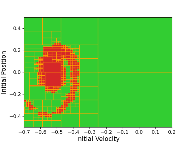
(b) Parameter space partitioning obtained using root split ($\delta_{\min}=0.02$)

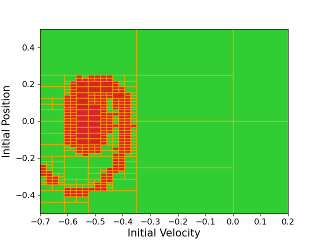
(c) Parameter space partitioning obtained using greatest uncertainty split ($\delta_{\min}=0.02$)

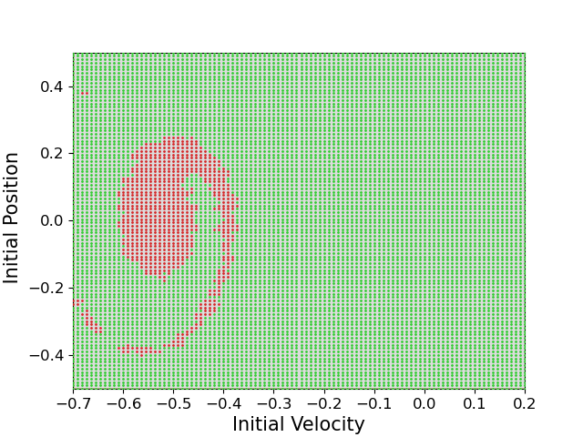
(d) Mountain Car Ground Truth

Figure 3: Mountain Car parameter space partitioning using different approaches

$\mathtt{Partition}$ method	# covers	Ratio of Volumes (%)
		Safe	Unsafe	Unk.
Naïve (Section 3.3)	457	89.01	10.99	0.00
Root split	481	89.23	10.77	0.00
Greatest uncertainty	364	88.72	11.28	0.00

Table 2: Comparison of Algorithm 2 using different $\mathtt{Partition}$ approaches with 95% confidence level.

We compare with approximate ground truth obtained by uniform sampling of the parameter space in Fig. 3d. Green dots indicate parameter values that lead to satisfaction of the property, while red dots indicate violations. In Fig. 3a 3b 3c, we show the results obtained using Algorithm 2. Table 2 summaries the parameter space partitioning results where green regions correspond to parameters that leads to satisfaction of $\varphi_{\textsc{mc}}$, and red regions correspond to parameters that leads to violation of $\varphi_{\textsc{mc}}$. Although the partition covers look different using the different partitioning strategies, the safe/unsafe ratio remain similar and they all provide the same level of probabilistic guarantees. Among the three partitioning approaches, we have the least number of total covers using the greatest uncertainty split method. In general, less number of covers lead to less number of simulations.

Reinforcement Learning Lane Keep Assist.

Lane-keep assist (LKA) is an automated driver assistance technique used in semi autonomous vehicles to keep the ego vehicle traveling along the centerline of a lane. The recent reinforcement learning toolbox from Matlab^® introduces a Deep Q Network (DQN)-based reinforcement learning agent that seeks to keep the ego vehicle centered. The inputs to the RL agent are the lateral deviation $e_{1}$, relative yaw angle (i.e. yaw error) $e_{2}$, their derivatives and their integrals. Specifics of the DQN-based RL agent and its training can be found in [29]. The parameter space for this model is the initial values for $e_{1}$ and $e_{2}$, where we looked at region $\Theta=(e_{1},e_{2})\in[-0.3,0.3]\times[-0.2,0.2]$. We are interested in the signals corresponding to the lateral deviation and yaw error. We are interested in checking the control-theoretic properties such as overshoot/undershoot bounds and the settling time for these signals. In this experiment, we consider two properties characterizing bounds on $e_{2}$ and settling time for $e_{1}$; $\varphi_{\textsc{lka},\mathrm{settle}}:\mathbf{G}_{[2,15]}(|e_{1}|<0.025)$ and $\varphi_{\textsc{lka},\mathrm{bounds}}:\mathbf{G}_{[0,15]}(e_{2}<0.4\wedge e_{2}>-0.4)$.

Figure 4 shows the parameter space partitioning results and the ground truth with respect to $\varphi_{\textsc{lka},\mathrm{settle}}$. Our technique was able to certify that $\varphi_{\textsc{lka},\mathrm{bounds}}$ is satisfied by the entire region with 95% confidence.

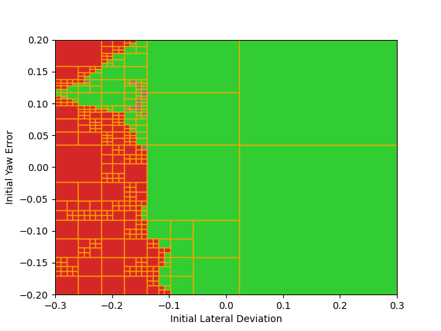
(a) Parameter space partitioning using greatest uncertainty split ($\delta_{\min}=0.01$)

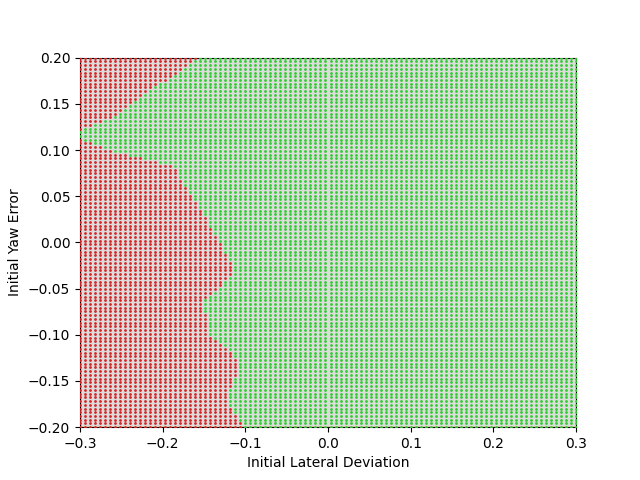
(b) LKA (settle) Ground Truth

Figure 4: Lane Keep Assist

F-16 Control System.

We now present the results of our technique on the verification challenge [16] which requires the analysis of the F-16 flight control loop system. The system is modeled as a hierarchical control system - an outer-loop autopilot and an inner loop tracking and stabilizing controller (ILC), and a $13$ dimensional non-linear dynamical plant model. The plant dynamics are based on a 6 degrees of freedom standard airplane model [37] represented by a system of $13$ ODEs describing the force equations, kinematics, moments and a first-order lag model for the afterburning turbofan engine. These ODEs describe the evolution of the system states, namely velocity $vt$, angle of attack $\alpha$, sideslip $\beta$, altitude $h$, attitude angles: roll $\phi$, pitch $\theta$, yaw $\psi$, and their corresponding rates $p$, $q$, $r$, engine $power$ and two more states for translation along north and east. The non-linear plant model uses linearly interpolated lookup tables to incorporate wind tunnel data. The control system is composed of an autopilot that sets the references on upward acceleration, stability roll rate and the $throttle$. The ILC uses an LQR state feedback law to track the references and computes the control input for the $aileron$, $rudder$ and the $elevator$. We now present our results on three separate scenarios capturing specific contexts. Each scenario defines the parameter set and an associated specification.

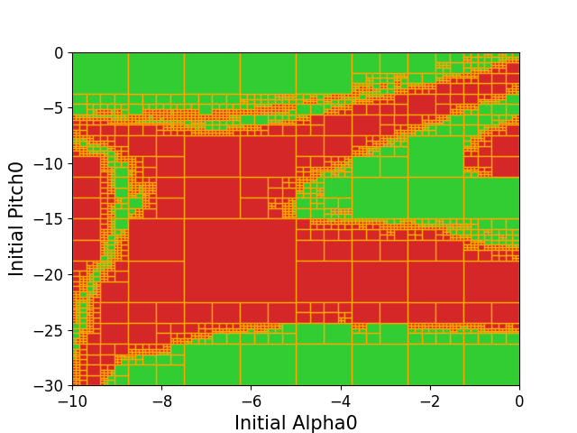
(a) Parameter space partitioning using greatest uncertainty split ($\delta_{\min}=0.1$)

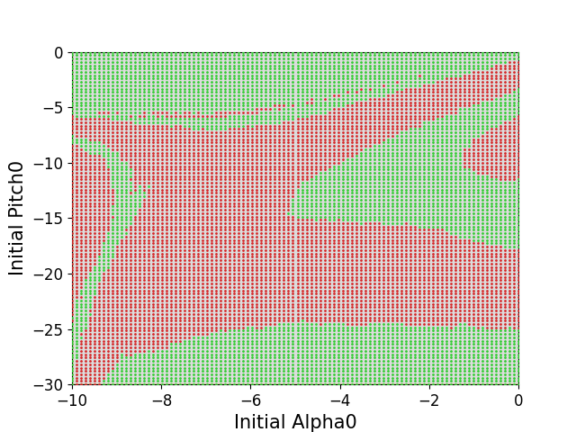
(b) Ground truth

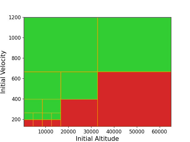
(c) Parameter space partitioning using greatest uncertainty split ($\delta_{\min}=100$)

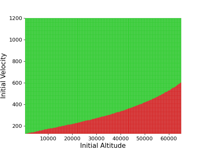
(d) Ground truth

Figure 5: F16 - Level Flight (bottom), Pull up maneuver (top)

F16-Pull up maneuver. This scenario demonstrates the tracking of a constant autopilot command requesting an upward acceleration ($N_{z}=5g$). The ILC tries to track the reference without undesirable transients like pitch oscillations and exceeding pitch rate limits. We modify the controller gains to highlight the violations of the spec $\phi_{\textsc{f16,pullup}}:\mathbf{G}_{[0,10]}q\leq 120deg/s$. The bounded parameter space is described by initial values of $\alpha\in[-10,0]deg,\theta\in[-30,0]deg$ and the results are shown in Figure 5a, 5b.

F16-Level Flight. This scenario describes straight and level flight with a constant attitude and $0$ initial angular rates. The bounded parameter space is defined by the initial altitude $h\in[500,65000]$ and velocity $vt\in[130,1200]$. The autopilot references are set to zero, and the ILC tries to maintain a constant altitude and angle of attack $\alpha$. As the F-16 can fly over a large range of altitudes and velocities, a single LQR computed against the linearzied model can not satisfy the goal and results in a stall defined by $\phi_{\textsc{f16,level}}:\mathbf{G}_{[0,10]}\alpha\leq 35deg$. This is reflected in the results as shown in Figure 5.

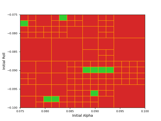
(a) Parameter space partitioning obtained using greatest uncertainty split ($\delta_{\min}$=0.002)

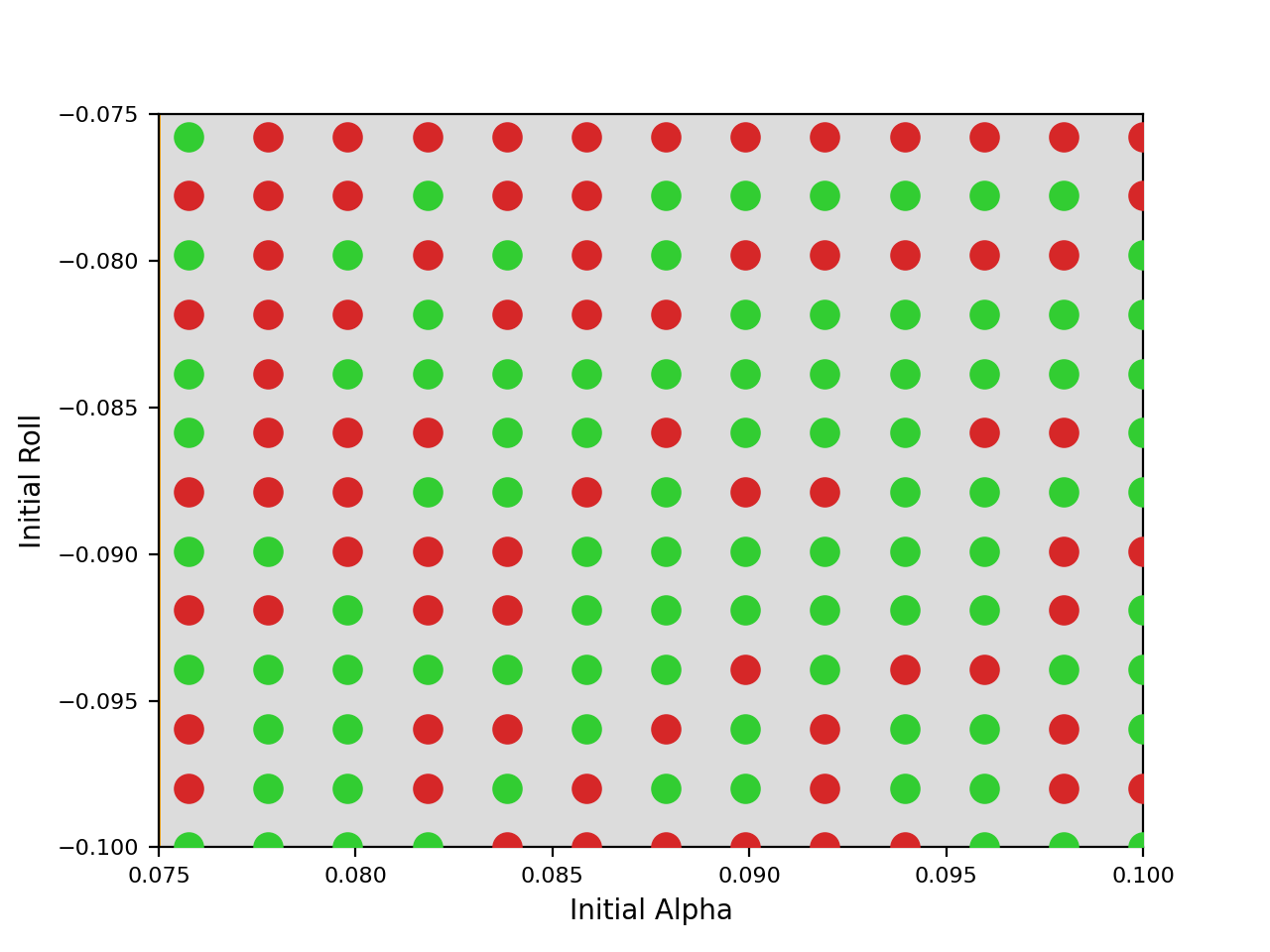
(b) GCAS Ground truth

Figure 7: F16 - Ground Collision Avoidance

F16-Ground Collision Avoidance(GCAS). The final scenario describes the F-16 diving towards the ground and the GCAS autopilot trying to prevent the collision. The GCAS brings the roll angle and its rate to $0$ and then accelerates upwards to avoid ground collision as defined by the spec $\phi_{\textsc{f16,gcas}}:\mathbf{G}_{[0,10]}h\geq 0ft$. The parameter space is described by initial values of $\alpha\in[0.075,0.1]rad$ and $\phi\in[-0.1,-0.075]rad$ . The results are illustrated in Figure 7. In this case study, the ground truth and our results seem to be less well-matched than other case studies. There are a couple of reasons for this. First, observe that the ground truth is highly non-monotonic. Given the nonlinearity of the ground truth, our conformal interval prediction errs on the side of safety and marks a region unsafe. To remedy this, we would have to increase the number of simulations per region used to train the GP regression model and possibly experiment with other regression models (such as a deep neural network regressor).

Artificial Pancreas.

Type-1 diabetes (juvenile diabetes) is a chronic condition caused by the inability of the pancreas to secrete the required amount of insulin. Simglucose [43] is a Python implementation of the FDA-approved Type-1 Diabetes simulator [27] which models glucose kinetics. We input a list of tuples of time and meal size to Simglucose and set the same scenario environment. Choosing patients in different age will result in different simulation trace. The parameter meal time is constrained to be strictly increasing and the last meal time to be less than 24. For each scenario, the simulator provides traces records for different blood indicators based on a given setting environment. We are interested in checking the property of blood glucose(BG), such as if the blood glucose will violate an upper limitation in a day. In this case study, we implement our technique on this system verification by setting alpha as 0.05 and delta as 0.5. Therefore, we present the results with 95% confidence guarantee and any subset size less than 0.5 is considered as an unknown region.

We study $4$ scenarios (Table 3) describing an adolescent patient who takes $2$,$3$,$4$ and $5$ meals a day respectively. The meals of size $s_{i}$ are consumed at time $t_{i}$. The parameters space is then defined by $\Theta=(t_{1},s_{1},\ldots,t_{i},s_{i},\ldots t_{n},s_{n})$, where $n$ is the total number of meals. The properties $\chi_{\textsc{simglucose},n\textsc{M}}:\mathbf{G}_{[0,T]}BG\leq UP$ (where $\chi\in{\phi,\psi}$), asserts that the patient’s blood glucose should not go beyond the upper bound ($UP$) in time $T$. Our results predict the whole region as $100\%$ safe region with $95\%$ confidence. Besides, for the two meal case: $\psi_{\textsc{simglucose,2M}}$, our implementation result of 54.44% matches well based on the ground truth dataset with 52.47% unsafe volume.

Specification	Unsafe Volume (Ground Truth) (%)
$\Theta_{2M}\in[1,12]\times[1,20]\times[13,24]\times[1,20]$
$\psi_{\textsc{simglucose,2M}}:\mathbf{G}_{[0,24]}BG\leq 155$	52.47
$\phi_{\textsc{simglucose,2M}}:\mathbf{G}_{[0,24]}BG\leq 170$	0
$\Theta_{3M}\in[1,8]\times[1,20]\times[9,16]\times[1,20]\times[17,24]\times[1,20]$
$\phi_{\textsc{simglucose,3M}}:\mathbf{G}_{[0,24]}BG\leq 170$	1.2
$\Theta_{4M}\in[1,6]\times[1,20]\times[7,12]\times[1,20]\times[13,18]\times[1,20]\times[19,24]\times[1,20]$
$\phi_{\textsc{simglucose,4M}}:\mathbf{G}_{[0,24]}BG\leq 170$	4.7
$\Theta_{5M}\in[1,4]\times[1,20]\times[5,9]\times[1,20]\times[10,14]\times[1,20]\times[15,19]\times[1,20]\times[20,24]\times[1,20]$
$\phi_{\textsc{simglucose,5M}}:\mathbf{G}_{[0,24]}BG\leq 170$	6.6

Table 3: Simglucose results with 95% confidence level for different parameter spaces and specifications.

Impact of Results. The parameter space partitioning produced by our algorithm helps characterize safe and unsafe regions of operation for CPS applications. This helps in selection of the appropriate model parameters or initial conditions during design time and runtime. Furthermore, if the model parameters are being chosen by an outer loop supervisory control, then the partitions that we generate create conditional contracts on the safety of the CPS model. Ultimately, we envision the results of our tool to be used for constructing safety assurance cases[35].

6 Related Work and Conclusions

Related Work. Several verification techniques for CPS have been proposed in the recent years. Some are specifically developed to analyze models of neural networks (NN) or NN-controlled dynamical systems in order to obtain safety guarantees, using barrier functions [34, 40], reachability analysis [39, 18, 19, 13], Satisfiability Modulo Theory (SMT) based methods or mixed-integer linear program (MILP) optimizer [21, 38, 10]. Most of these methods provide deterministic guarantees but face scalability issues and are restricted by the class of models they can handle (e.g. ReLU activation functions). Unlike these approaches, our method is applicable to a broader class of CPS as it treats learning-enabled CPS as black-boxes and only assumes that they can compute simulations given fixed parameters. Moreover, we reason over the joint distribution of the parameters and corresponding robust values with respect to STL properties. Therefore, our algorithm is independent of the model complexity (except for the computational complexity of the simulations) and more scalable.

Methods based on Statistical Model Checking (SMC) [22, 23, 46] can overcome the hurdles like scalability and nonlinearity and provide probabilistic guarantees [45, 33, 42, 7, 1]. These methods are based on statistical inference methods like sequential probability ratio tests [22, 33, 36, 7], Bayesian statistics [46], and Clopper-Pearson bounds [45]. Another line of works use Probably Approximately Correct (PAC) learning theory to give probabilistic bounds for Markov decision processes and black-box systems [15, 12]. In contrast to SMC and PAC-learning techniques, our approach is sample independent and can provide the required probabilistic guarantees with any number of samples. This is because we build a guaranteed regression model from the system parameters with respect to the robust satisfaction value of the corresponding STL properties. If the regression model is of poor quality (due to few samples), using the calibration step in conformal regression, the predicted (but wider) interval can still have the same level of guarantee. Conformal regression lets us tradeoff the quality of the regression model (w.r.t. the data) and the width of the interval for which we have high-confidence property satisfaction, and not the level of the guarantee itself.

Conclusions. In this paper, we proposed a verification framework that can search the parameter space to find the regions that lead to satisfaction or violation of given specification with probabilistic coverage guarantees. There are a couple of directions we aim to explore as future work: 1) We used a very basic version of conformal regression in Algorithm 1, which gives a constant confidence range $d$ across all $X$. Techniques based on quantile regression [32] and locally-weighed conformal [24] can make $d$ a function of $X$ and give much shorter prediction intervals. 2) We plan to explore probabilistic regret bounds for Gaussian process optimization to help obtain (probabilistic) upper and lower bounds on the value of the surrogate model when using GP-based regression.

Appendix

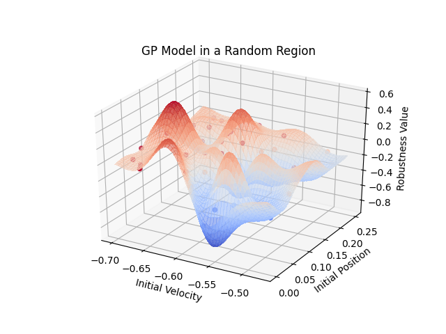
Figure 6: Gaussian Process Regression Visualization for the Mountain Car model

References

- [1] Abbas, H., Hoxha, B., Fainekos, G., Ueda, K.: Robustness-guided temporal logic testing and verification for stochastic cyber-physical systems. In: The 4th Annual IEEE International Conference on Cyber Technology in Automation, Control and Intelligent Systems. pp. 1–6. IEEE (2014)
- [2] Agha, G., Palmskog, K.: A survey of statistical model checking. ACM Transactions on Modeling Computing and Simululation 28(1), 6:1–6:39 (2018). https://doi.org/10.1145/3158668, https://doi.org/10.1145/3158668
- [3] Akazaki, T., Hasuo, I.: Time Robustness in MTL and Expressivity in Hybrid System Falsification. In: CAV. pp. 356–374. Lecture Notes in Computer Science (2015)
- [4] Barron, A.R.: Universal approximation bounds for superpositions of a sigmoidal function. IEEE Transactions on Information theory 39(3), 930–945 (1993)
- [5] Bishop, C.M.: Pattern recognition and machine learning. springer (2006)
- [6] Cerny, P., Henzinger, T.A., Radhakrishna, A.: Quantitative abstraction refinement. In: Proceedings of the 40th annual ACM SIGPLAN-SIGACT symposium on Principles of programming languages. pp. 115–128 (2013)
- [7] Clarke, E.M., Faeder, J.R., Langmead, C.J., Harris, L.A., Jha, S.K., Legay, A.: Statistical model checking in biolab: Applications to the automated analysis of t-cell receptor signaling pathway. In: CMSB. pp. 231–250. Springer (2008)
- [8] Donzé, A., Maler, O.: Robust satisfaction of temporal logic over real-valued signals. In: FORMATS. pp. 92–106. Springer (2010)
- [9] Dreossi, T., Fremont, D.J., Ghosh, S., Kim, E., Ravanbakhsh, H., Vazquez-Chanlatte, M., Seshia, S.A.: Verifai: A toolkit for the formal design and analysis of artificial intelligence-based systems. In: CAV. pp. 432–442. Springer International Publishing, Cham (2019)
- [10] Dutta, S., Jha, S., Sankaranarayanan, S., Tiwari, A.: Learning and verification of feedback control systems using feedforward neural networks. IFAC-PapersOnLine 51(16), 151–156 (2018)
- [11] Fainekos, G.E., Pappas, G.J.: Robustness of temporal logic specifications for continuous-time signals. Theoretical Computer Science 410(42), 4262–4291 (2009)
- [12] Fan, C., Qi, B., Mitra, S., Viswanathan, M.: Dryvr: Data-driven verification and compositional reasoning for automotive systems. In: CAV. pp. 441–461 (2017)
- [13] Fazlyab, M., Robey, A., Hassani, H., Morari, M., Pappas, G.: Efficient and accurate estimation of lipschitz constants for deep neural networks. In: NeurIPS. pp. 11423–11434 (2019)
- [14] Friedman, J., Hastie, T., Tibshirani, R.: The elements of statistical learning, vol. 1. Springer series in statistics New York (2001)
- [15] Fu, J., Topcu, U.: Probably approximately correct mdp learning and control with temporal logic constraints. arXiv preprint arXiv:1404.7073 (2014)
- [16] Heidlauf, P., Collins, A., Bolender, M., Bak, S.: Verification challenges in f-16 ground collision avoidance and other automated maneuvers. In: ARCH@ ADHS. pp. 208–217 (2018)
- [17] Hoxha, B., Bach, H., Abbas, H., Dokhanchi, A., Kobayashi, Y., Fainekos, G.: Towards formal specification visualization for testing and monitoring of cyber-physical systems. In: Int. Workshop on Design and Implementation of Formal Tools and Systems. sn (2014)
- [18] Huang, X., Kwiatkowska, M., Wang, S., Wu, M.: Safety verification of deep neural networks. In: International Conference on Computer Aided Verification. pp. 3–29. Springer (2017)
- [19] Ivanov, R., Weimer, J., Alur, R., Pappas, G.J., Lee, I.: Verisig: Verifying safety properties of hybrid systems with neural network controllers. In: HSCC (2019)
- [20] Jakšić, S., Bartocci, E., Grosu, R., Nguyen, T., Ničković, D.: Quantitative monitoring of STL with edit distance. Formal Methods in System Design 53(1), 83–112 (Aug 2018). https://doi.org/10.1007/s10703-018-0319-x
- [21] Katz, G., Barrett, C., Dill, D.L., Julian, K., Kochenderfer, M.J.: Reluplex: An efficient smt solver for verifying deep neural networks. In: Majumdar, R., Kunčak, V. (eds.) Computer Aided Verification. pp. 97–117. Springer International Publishing, Cham (2017)
- [22] Legay, A., Delahaye, B., Bensalem, S.: Statistical model checking: An overview. In: Runtime Verification. pp. 122–135. Springer Berlin Heidelberg, Berlin, Heidelberg (2010)
- [23] Legay, A., Viswanathan, M.: Statistical model checking: challenges and perspectives (2015)
- [24] Lei, J., G’Sell, M., Rinaldo, A., Tibshirani, R.J., Wasserman, L.: Distribution-free predictive inference for regression. Journal of the American Statistical Association 113(523), 1094–1111 (2018)
- [25] Lei, J., Wasserman, L.: Distribution-free prediction bands for non-parametric regression. Journal of the Royal Statistical Society: Series B (Statistical Methodology) 76(1), 71–96 (2014)
- [26] Maler, O., Nickovic, D.: Monitoring temporal properties of continuous signals. In: FORMATS, pp. 152–166. Springer (2004)
- [27] Man, C.D., Micheletto, F., Lv, D., Breton, M., Kovatchev, B., Cobelli, C.: The uva/padova type 1 diabetes simulator: new features. Journal of diabetes science and technology 8(1), 26–34 (2014)
- [28] Mooney, C.Z.: Monte carlo simulation, vol. 116. Sage publications (1997)
- [29] R2020a, M.: Train dqn agent for lane keep assist. https://www.mathworks.com/help/reinforcement-learning/ug/train-dqn-agent-for-lane-keeping-assist.html, the Mathworks
- [30] Rasmussen, C.E.: Gaussian processes in machine learning. In: Summer School on Machine Learning. pp. 63–71. Springer (2003)
- [31] Rodionova, A., Bartocci, E., Nickovic, D., Grosu, R.: Temporal Logic as Filtering. Proceedings of the 19th International Conference on Hybrid Systems: Computation and Control - HSCC ’16 pp. 11–20 (2016)
- [32] Romano, Y., Patterson, E., Candes, E.: Conformalized quantile regression. In: NeurIPS. pp. 3538–3548 (2019)
- [33] Roohi, N., Wang, Y., West, M., Dullerud, G.E., Viswanathan, M.: Statistical verification of the toyota powertrain control verification benchmark. In: Proceedings of the 20th International Conference on Hybrid Systems: Computation and Control. pp. 65–70. HSCC ’17, Association for Computing Machinery, New York, NY, USA (2017). https://doi.org/10.1145/3049797.3049804
- [34] Royo, V.R., Fridovich-Keil, D., Herbert, S.L., Tomlin, C.J.: Classification-based approximate reachability with guarantees applied to safe trajectory tracking. ArXiv abs/1803.03237 (2018)
- [35] Rushby, J.: Partitioning for safety and security: Requirements, mechanisms, and assurance. AFRL-IF-RS-TR’-2002-85 p. 9 (2002)
- [36] Sen, K., Viswanathan, M., Agha, G.: Statistical model checking of black-box probabilistic systems. In: Alur, R., Peled, D.A. (eds.) Computer Aided Verification. pp. 202–215. Springer Berlin Heidelberg, Berlin, Heidelberg (2004)
- [37] Stevens, B.L., Lewis, F.L., Johnson, E.N.: Aircraft control and simulation: dynamics, controls design, and autonomous systems. John Wiley & Sons (2015)
- [38] Sun, X., Khedr, H., Shoukry, Y.: Formal verification of neural network controlled autonomous systems. In: Proceedings of the 22nd ACM International Conference on Hybrid Systems: Computation and Control. p. 147–156. HSCC ’19, Association for Computing Machinery, New York, NY, USA (2019). https://doi.org/10.1145/3302504.3311802
- [39] Tran, H.D., Manzanas Lopez, D., Musau, P., Yang, X., Nguyen, L.V., Xiang, W., Johnson, T.T.: Star-based reachability analysis of deep neural networks. In: ter Beek, M.H., McIver, A., Oliveira, J.N. (eds.) Formal Methods – The Next 30 Years. pp. 670–686. Springer International Publishing, Cham (2019)
- [40] Tuncali, C.E., Kapinski, J., Ito, H., Deshmukh, J.V.: Reasoning about safety of learning-enabled components in autonomous cyber-physical systems. In: Proceedings of the 55th Annual Design Automation Conference. DAC ’18, Association for Computing Machinery, New York, NY, USA (2018). https://doi.org/10.1145/3195970.3199852
- [41] Vovk, V., Gammerman, A., Shafer, G.: Algorithmic learning in a random world. Springer Science & Business Media (2005)
- [42] Wang, Y., Zarei, M., Bonakdarpour, B., Pajic, M.: Statistical verification of hyperproperties for cyber-physical systems. ACM Trans. Embed. Comput. Syst. 18(5s) (Oct 2019). https://doi.org/10.1145/3358232, https://doi.org/10.1145/3358232
- [43] Xie, J.: Simglucose v0.2.1. https://github.com/jxx123/simglucose (2018)
- [44] Yaghoubi, S., Fainekos, G.: Gray-box adversarial testing for control systems with machine learning components. In: Proceedings of the 22nd ACM International Conference on Hybrid Systems: Computation and Control. pp. 179–184 (2019)
- [45] Zarei, M., Wang, Y., Pajic, M.: Statistical verification of learning-based cyber-physical systems. In: Proceedings of the 23nd ACM International Conference on Hybrid Systems: Computation and Control (2020)
- [46] Zuliani, P., Platzer, A., Clarke, E.M.: Bayesian statistical model checking with application to simulink/stateflow verification. In: Proceedings of the 13th ACM international conference on Hybrid systems: computation and control. pp. 243–252 (2010)