Anisotropic and crystalline mean curvature flow of mean-convex sets

Abstract

We consider a variational scheme for the anisotropic and crystalline mean curvature flow of sets with strictly positive anisotropic mean curvature. We show that such condition is preserved by the scheme, and we prove the strict convergence in $BV$ of the time-integrated perimeters of the approximating evolutions, extending a recent result of De Philippis and Laux to the anisotropic setting. We also prove uniqueness of the flat flow obtained in the limit.

Keywords: Anisotropic mean curvature flow, crystal growth, minimizing movements, mean convexity, arrival time, $1$-superharmonic functions.

MSC (2020): 53E10, 49Q20, 58E12, 35A15, 74E10.

1 Introduction

We are interested in the anisotropic mean curvature flow of sets with positive anisotropic mean curvature. More precisely, following [14, 12] we consider a family of sets $t\mapsto E(t)$ governed by the geometric evolution law

$$V(x,t)=-\psi(\nu_{E(t)})\,\kappa_{E(t)}^{\phi}(x),$$ (1)

where $V(x,t)$ denotes the normal velocity of the boundary $\partial E(t)$ at $x$, $\phi$ is a given norm or, more generally, a possibly non-symmetric convex, one-homogeneous function on $\mathbb{R}^{d}$, $\kappa_{E(t)}^{\phi}$ is the anisotropic mean curvature of $\partial E(t)$ associated with the anisotropy $\phi$, and $\psi$ is another convex, one-homogeneous function, usually called mobility, evaluated at the outer unit normal $\nu_{E(t)}$ to $\partial E(t)$. Both $\phi$ and $\psi$ are real-valued and positive away from $0$. We recall that when $\phi$ is differentiable in $\mathbb{R}^{d}\setminus\{0\}$, then $\kappa_{E}^{\phi}$ is given by the tangential divergence of the so-called Cahn-Hoffman vector field [8]

$$\kappa_{E}^{\phi}=\textup{div}\,_{{\tau}}\left(\nabla\phi(\nu_{E})\right),$$ (2)

while in general (2) should be replaced with the differential inclusion

$$\kappa_{E}^{\phi}=\textup{div}\,_{{\tau}}\left(n_{E}^{\phi}\right),\qquad n_{E}^{\phi}\in\partial\phi(\nu_{E}).$$

It is well-known that (1) can be interpreted as gradient flow of the anisotropic perimeter

$$P_{\phi}(E)=\int_{\partial E}\phi(\nu_{E})d\mathcal{H}^{d-1}\,,$$

and one can construct global-in-time weak solutions by means of the variational scheme introduced by Almgren, Taylor and Wang [3] and, independently, by Luckhaus and Sturzenhecker [18]. Such scheme consists in building a family of tme-discrete evolutions by an iterative minimization procedure and in considering any limit of these discrete evolutions, as the time step $h>0$ vanishes, as an admissible solution to the geometric motion, usually referred to as a flat flow. The problem which is solved at each step takes the form [3, §2.6] $E_{h}^{n}:=T_{h}E_{h}^{n-1}$, where $T_{h}E$ is a solution of

$$\min_{F}P_{\phi}(F)+\frac{1}{h}\int_{F}d^{{\psi^{\circ}}}_{E}(x)dx,$$ (3)

where $d^{{\psi^{\circ}}}_{E}$ is the signed distance function of $E$, with respect to the anisotropy ${\psi^{\circ}}$, which is defined as

$$d^{\psi^{\circ}}_{E}(x):=\inf_{y\in E}{\psi^{\circ}}(x-y)-\inf_{y\not\in E}{\psi^{\circ}}(y-x).$$ (4)

In [3] it is proved that the discrete solution $E_{h}(t):=E_{h}^{[\frac{t}{h}]}$, with $\psi=1$ and $\phi$ smooth, converges to a limit flat flow which is contained in the zero-level set of the (unique) viscosity solution of (1). Such a result has been extended in [14, 12] to general anisotropies $\psi,\phi$. In the isotropic case $\phi=\psi=|\cdot|$ it is shown in [18] that $E_{h}(t)$ converges to a distributional solution $E(t)$ of (1), under the assumption that the perimeter is continuous in the limit, that is,

$$\lim_{h\to 0}\int_{0}^{T}P(E_{h}(t))\,dt=\int_{0}^{T}P(E(t))\qquad\text{for }T>0.$$ (5)

Recently, it has been shown in [15] that the continuity of the perimeter holds if the initial set is outward minimizing for the perimeter (see Section 2.1), a condition which implies the mean convexity and which is preserved by the variational scheme (3).

In this paper we generalize the result in [15] to the general anisotropic case, where the continuity of the perimeter was previously known only in the convex case [7], as a consequence of the convexity preserving property of the scheme. Such result is obtained under a stronger condition of strong outward minimality of the initial set, which is also preserved by the scheme and implies the strict positivity of the anisotropic mean curvature. As a corollary, we obtain the continuity of the volume and of the (anisotropic) perimeter of the limit flat flow.

The plan of the paper is the following: In Section 2 we introduce the notion of outward minimizing set, and we recall the variational scheme proposed by Almgren, Taylor and Wang in [3]. We also show that the scheme preserves the strict outward minimality. In section 3 we show the strict $BV$-convergence of the discrete arrival time functions, we prove the uniqueness of the limit flow, and we show continuity in time of volume and perimeter, and in Section 4 we give some examples. Eventually, in Appendix A we recall some results on $1$-superharmonic functions, adapted to the anisotropic setting.

2 Preliminary definitions

2.1 Outward minimizing sets

Definition 2.1.

Let $\Omega$ be an open subset of $\mathbb{R}^{d}$ and let $E\subset\subset\Omega$ be a finite perimeter set. We say that $E$ is outward minimizing in $\Omega$ if

$$P_{\phi}(E)\leq P_{\phi}(F)\quad\forall F\supset E,F\subset\subset\Omega.$$

Note that, if $E$, $\phi$ are regular, $(MC)$ implies that the $\phi$-mean curvature of $\partial E$ is non-negative.

We observe that such a set satisfies the following density bound: There exists $\gamma>0$ such that, for all points $x\in E$ satisfying $|B(x,\rho)\setminus E|>0$ for all $\rho>0$, it holds:

$$\frac{|B(x,\rho)\setminus E|}{|B(x,\rho)|}\geq\gamma,$$ (6)

whenever $B(x,\rho)\subset\Omega$. As a consequence, whenever $x\in E$ is a point of Lebesgue density $1$, there exists $\rho>0$ small enough such that $|B(x,\rho)\setminus E|=0$. Therefore, identifying the set $E$ with its points of density $1$, we always assume (unless otherwise explicitly stated) that $E$ is an open subset of $\mathbb{R}^{d}$.

Conversely if $E\subset\mathbb{R}^{d}$ is bounded and $C^{2}$, $\phi$ is $C^{2}(\mathbb{R}^{d}\setminus\{0\})$, and its mean curvature is positive, then one can find $\Omega\supset\supset E$ such that $E$ is outward minimizing in $\Omega$. More precisely, if $E$ is of class $C^{2}$ then, in a neighborhood of $\partial E$, $d^{\phi^{\circ}}_{E}$ is $C^{2}$, while in a smaller neighborhood we even have $\textup{div}\,\nabla\phi(\nabla d^{\phi^{\circ}}_{E})\geq\delta$, for some $\delta>0$. Let $\Omega$ be the union of $E$ and this neighborhood, and set $n_{E}^{\phi}:=\nabla\phi(\nabla d^{\phi^{\circ}}_{E})$: then if $E\subset F\subset\subset\Omega$,

$$P_{\phi}(F)\geq\int_{\partial^{*}F}n^{\phi}_{E}\cdot\nu_{F}d\mathcal{H}^{d-1}=-\int_{\Omega}n^{\phi}_{E}\cdot D\chi_{F}$$

while by construction $P_{\phi}(E)=-\int_{\Omega}n^{\phi}_{E}\cdot D\chi_{E}$. Hence,

$$P_{\phi}(F)\geq P_{\phi}(E)-\int_{\Omega}n^{\phi}_{E}\cdot D(\chi_{F}-\chi_{E})=P_{\phi}(E)+\int_{F\setminus E}\textup{div}\,n^{\phi}_{E}\geq P_{\phi}(E)+\delta|F\setminus E|.$$

Observe (see [15, Lemma 2.5]) that equivalently, one can express this as:

$$P_{\phi}(E\cap F)\leq P_{\phi}(F)-\delta|F\setminus E|\quad\forall F\subset\subset\Omega.$$

Clearly, condition $(MC_{\delta})$ is stronger and reduces to $(MC)$ whenever $\delta=0$.

Remark 2.2 (Non-symmetric distances).

As in the standard case (that is when ${\psi^{\circ}}$ is smooth and even), the signed “distance” function defined in (4) is easily seen to satisfy the usual properties of a signed distance function. First, it is Lipschitz continuous, hence differentiable almost everywhere. Then, if $x$ is a point of differentiability, $d^{\psi^{\circ}}_{E}(x)>0$ and $y\in\partial E$ is such that ${\psi^{\circ}}(x-y)=d^{\psi^{\circ}}_{E}(x)$, then for $s>0$ small and $h\in\mathbb{R}^{d}$ $d^{\psi^{\circ}}_{E}(x+sh)\geq{\psi^{\circ}}(x+sh-y)\geq{\psi^{\circ}}(x-y)+sz\cdot h$ for any $z\in\partial{\psi^{\circ}}(x-y)$ and one deduces that $\partial{\psi^{\circ}}(x-y)=\{\nabla d^{\psi^{\circ}}_{E}(x)\}$. If $d^{\psi^{\circ}}_{E}(x)<0$, one writes that ${\psi^{\circ}}(y-x)=-d^{\psi^{\circ}}_{E}(x)$ for some $y\in\partial E$ and uses ${\psi^{\circ}}(y-x-sh)\geq{\psi^{\circ}}(y-x)-sz\cdot h$ for some $z\in\partial{\psi^{\circ}}(y-x)$, hence $d^{\psi^{\circ}}_{E}(x+sh)-d^{p}_{E}(x)\leq sz\cdot h$ to deduce now that $\partial{\psi^{\circ}}(y-x)=\{\nabla d^{\psi^{\circ}}_{E}(x)\}$. In all cases, one has $\psi(\nabla d^{\psi^{\circ}}_{E}(x))=1$ a.e. in $\{d^{\psi^{\circ}}_{E}\neq 0\}$ (while of course $\nabla d^{\psi^{\circ}}_{E}(x)=0$ a.e. in $\{d^{\psi^{\circ}}_{E}=0\}$), and $\nabla d^{\psi^{\circ}}_{E}(x)\cdot(x-y)=d^{\psi^{\circ}}_{E}(x)$, which shows that $y\in x-d^{\psi^{\circ}}_{E}(x)\partial\phi(\nabla d^{\psi^{\circ}}_{E}(x))$).

2.2 The discrete scheme

We now consider here the discrete scheme introduced in [18, 3] and its generalization in [11, 7, 14, 13]. It is based on the following process: given $h>0$, and $E$ a (bounded) finite perimeter set, we define $T_{h}E$ as a minimizer of

$$\min_{F}P_{\phi}(F)+\frac{1}{h}\int_{F}d_{E}^{\psi^{\circ}}(x)dx$$

where $d^{\psi^{\circ}}_{E}$ is defined in (4). If $E\subset\subset\Omega$ satisfies $(MC)$ in $\Omega$, it is clear that for $h>0$ small enough, one has $T_{h}E\subset E$. Indeed, for $h$ small enough one has $\overline{T_{h}E}\subset\Omega$, and it follows from $(MC)$ (more precisely, in the form $(MC_{\delta})$ for $\delta=0$) that

$$P_{\phi}(T_{h}E\cap E)+\frac{1}{h}\int_{T_{h}E\cap E}d^{\psi^{\circ}}_{E}(x)dx\leq P_{\phi}(T_{h}E)+\frac{1}{h}\int_{T_{h}E}d^{\psi^{\circ}}_{E}(x)dx-\frac{1}{h}\int_{T_{h}E\setminus E}d^{\psi^{\circ}}_{E}(x)dx,$$ (7)

which implies that $|T_{h}E\setminus E|=0$. We recall in addition that in this case, $T_{h}E$ is also $\phi$-mean convex in $\Omega$, see the proof of [15, Lemma 2.7]. If $E$ satisfies $(MC_{\delta})$ in $\Omega$ for some $\delta>0$, we can improve the inclusion $T_{h}E\subset E$.

Lemma 2.3.

Assume that $E\subset\subset\Omega$ satisfies $(MC_{\delta})$ in $\Omega$, for some $\delta>0$. Then for $h>0$ small enough, it holds

$$T_{h}E+\{{\psi^{\circ}}\leq\delta h\}\subset E.$$

In particular, $d^{\psi^{\circ}}_{T_{h}E}\geq d^{\psi^{\circ}}_{E}+\delta h$ and $T_{h}E\subset\{d^{\psi^{\circ}}_{E}\leq-\delta h\}$.

Proof.

Let $h>0$ small enough so that $T_{h}E\subset E$ and $E+\{{\psi^{\circ}}\leq\delta h\}\subset\Omega$. Choose $\tau$ with ${\psi^{\circ}}(\tau)<\delta h$ and consider $F:=T_{h}E+\tau$. We show that also $F\subset E$. The set $F\subset\subset\Omega$ is a minimizer of

$$P_{\phi}(F)+\frac{1}{h}\int_{F}d^{\psi^{\circ}}_{E}(x-\tau)dx.$$

In particular, we have

$$P_{\phi}(F)+\frac{1}{h}\int_{F}d^{\psi^{\circ}}_{E}(x-\tau)dx\leq P_{\phi}(F\cap E)+\frac{1}{h}\int_{F\cap E}d^{\psi^{\circ}}_{E}(x-\tau)dx\\ \leq P_{\phi}(F)+\frac{1}{h}\int_{F}d^{\psi^{\circ}}_{E}(x-\tau)dx-\int_{F\setminus E}\frac{1}{h}d^{\psi^{\circ}}_{E}(x-\tau)+\delta\,dx.$$

By definition of the signed distance function, for $x\not\in E$, $d^{\psi^{\circ}}_{E}(x-\tau)\geq-{\psi^{\circ}}(x-(x-\tau))=-{\psi^{\circ}}(\tau)>-\delta h$ so that if $|F\setminus E|>0$ we have a contradiction. We deduce that $T_{h}E+\{{\psi^{\circ}}\leq\delta h\}\subset E$.

In particular, if $x\in T_{h}E$ and $y\not\in E$ is such that $d^{\psi^{\circ}}_{E}(x)=-{\psi^{\circ}}(y-x)$, then $y^{\prime}=y-\delta h(y-x)/{\psi^{\circ}}(y-x)\not\in T_{h}E$ hence $d^{\psi^{\circ}}_{T_{h}E}\geq-{\psi^{\circ}}(y^{\prime}-x)=d^{\psi^{\circ}}_{E}(x)-\delta h$. If $x\in E\setminus T_{h}E$, $d^{\psi^{\circ}}_{E}(x)=-\psi(y-x)$ for some $y\in\overline{\Omega\setminus E}$, and $d_{T_{h}E}^{\psi^{\circ}}(x)=\psi(x-y^{\prime})$ for some $y^{\prime}\in T_{h}E$. Since $\psi(x-y^{\prime})+\psi(y-x)\geq\psi(y-y^{\prime})\geq\delta h$ we conclude. Eventually if $x\not\in E$, for $y\in T_{h}E$ with $d^{\psi^{\circ}}_{T_{h}E}(x)={\phi^{\circ}}(x-y)$ we have $y+\delta h(x-y)/{\phi^{\circ}}(x-y)\in E$, so that $d^{\psi^{\circ}}_{E}(x)\leq{\phi^{\circ}}(x-y)-\delta h=d^{\psi^{\circ}}_{T_{h}E}(x)-\delta h$. This shows that $d^{\psi^{\circ}}_{T_{h}E}\geq d^{\psi^{\circ}}_{E}+\delta h$. ∎

Corollary 2.4.

Under the assumptions of Lemma 2.3, for any $n\geq 1$, we have $T_{h}^{n+1}E+\{{\psi^{\circ}}\leq\delta h\}\subset T_{h}^{n}E$ and $d^{\psi^{\circ}}_{T_{h}^{n}E}\geq d^{\psi^{\circ}}_{E}+\delta nh.$

Proof.

The first statement is obvious by induction: Assuming that for $\tau$ with ${\psi^{\circ}}(\tau)\leq\delta h$ one has $T_{h}^{n}E+\tau\subset T_{h}^{n-1}E$ which is true for $n=1$, applying $T_{h}$ again and using the translational invariance we get that $T_{h}^{n+1}E+\tau\subset T_{h}^{n}E$. The second statement is obviously deduced. Indeed we can reproduce the end of the previous proof to find that $d^{\psi^{\circ}}_{T_{h}^{n}E}\geq d^{\psi^{\circ}}_{T_{h}^{n-1}E}+\delta h$, the conclusion follows by induction. ∎

Remark 2.5 (Density estimates).

There exists $\gamma>0$, depending only on $\phi$ and the dimension, and $r_{0}>0$, depending also on $\psi$, such that the following holds: for $x$ such that $|B(x,r)\cap T_{h}E|>0$ for all $r>0$ one has $|B(x,r)\cap T_{h}E|\geq\gamma r^{d}$ if $r<r_{0}h$. For the complement, as $T_{h}E$ is $\phi$-mean convex in $\Omega$, we have as before that for $x$ such that $|B(x,r)\setminus T_{h}E|>0$ for all $r>0$, one has $|B(x,r)\setminus T_{h}E|\geq\gamma r^{d}$ for all $r$ with $B(x,r)\subset\Omega$, cf (6).

2.3 Preservation of the outward minimality

In the sequel, we show some further properties of the discrete evolutions and their limit. An interesting result in [15] is that the $(MC_{\delta})$-condition is preserved during the evolution. We prove that it is also the case in the anisotropic setting.

We first show the following result:

Lemma 2.6.

Let $\delta>0$ be such that there exists a set $E\subset\subset\Omega$ satisfying $(MC_{\delta})$ in $\Omega$. Then $\delta|F|\leq P_{\phi}(F)$ for any $F\subset\subset\Omega$, that is, the empty set also satisfies $(MC_{\delta})$ in $\Omega$.

Proof.

By $(MC_{\delta})$ we have $\delta|F|=\delta|F\cap E|+\delta|F\setminus E|\leq\delta|F\cap E|+(P_{\phi}(F)-P_{\phi}(F\cap E))$, so that it is enough to show the result for $F\subset E$. For $s>0$, we let $E_{s}$ be the largest minimizer of

$$P_{\phi}(E_{s})+\frac{1}{s}\int_{E_{s}}d^{\psi^{\circ}}_{E}\,dx,$$ (8)

which is obtained as the level set $\{w_{s}\leq 0\}$ of the (Lipschitz continuous) solution $w_{s}$ of the equation

$$-s\textup{div}\,z_{s}+w_{s}=d^{\psi^{\circ}}_{E},\quad z_{s}\in\partial\phi(\nabla w_{s}),$$ (9)

see for instance [11, 1] for details. A standard translation argument shows that the function $w_{s}$ satisfies $\psi(\nabla w_{s})\leq\psi(\nabla d_{E}^{\psi^{\circ}})=1$ a.e. in $\mathbb{R}^{d}$. We also let $E^{\prime}_{s}:=\{w_{s}<0\}$ be the smallest minimizer of (8). By construction, the set $E_{s}$ is closed while $E^{\prime}_{s}$ is open.

By Lemma 2.3 it follows that there exists $s_{0}>0$ such that $E_{s}\subset\subset E$ for all $s<s_{0}$. Moreover, being $E$ an open set, we also have $|E_{s}\Delta E|\to 0$ as $s\to 0$. Indeed, given $x,\rho$ with $B(x,\rho)\subset E$, by comparison we have that $x\in E_{s}$ for all $s<c\rho^{2}$, where $c>0$ depends only on $d,\phi$ and ${\psi^{\circ}}$.

Since $P_{\phi}(E_{s})\leq P_{\phi}(E)$, by the lower semicontinuity of $P_{\phi}$ we get that $\lim_{s\to 0}P_{\phi}(E_{s})=P_{\phi}(E).$ We also claim that

$$\lim_{s\to 0}P_{\phi}(F\cap E_{s})=P_{\phi}(F).$$ (10)

Indeed, it holds

$$P_{\phi}(F\cup E_{s})+P_{\phi}(F\cap E_{s})\leq P_{\phi}(E_{s})+P_{\phi}(F),$$

and $|E\setminus(F\cup E_{s})|\to 0$ as $s\to 0$, so that

$$P_{\phi}(E)+\limsup_{s\to 0}P_{\phi}(F\cap E_{s})\leq\limsup_{s\to 0}\left(P_{\phi}(F\cup E_{s})+P_{\phi}(F\cap E_{s})\right)\leq P_{\phi}(E)+P_{\phi}(F),$$

which shows the claim.

Again by Lemma 2.3 we know that $d_{E}^{\psi^{\circ}}\leq-s\delta$ on $\partial E_{s}=\{w_{s}\leq 0\}$. If $x\in E_{s}$ and $y\in\partial E_{s}$, $w_{s}(x)\geq w_{s}(y)-{\psi^{\circ}}(y-x)=-{\psi^{\circ}}(y-x)$ (using $\psi(\nabla w_{s})\leq 1$). If $z\not\in E$ and $y\in[x,z]\cap\partial E_{s}$, by one-homogeneity of ${\psi^{\circ}}$ we get one has ${\psi^{\circ}}(z-x)={\psi^{\circ}}(z-y)+{\psi^{\circ}}(y-x)$, so that $0\leq w_{s}(x)+{\psi^{\circ}}(y-x)=w_{s}(x)+{\psi^{\circ}}(z-x)-{\psi^{\circ}}(z-y)\leq w_{s}(x)+{\psi^{\circ}}(z-x)-s\delta$. Taking the infimum over $z$, we see that $s\delta\leq w_{s}(x)-d^{\psi^{\circ}}_{E}(x)$. Hence $\textup{div}\,z_{s}\geq\delta$ a.e. in $E_{s}$, so that

$$P_{\phi}(F\cap E_{s})\geq\int_{\Omega}\textup{div}\,z_{s}\chi_{F\cap E_{s}}\geq\delta|F\cap E_{s}|.$$ (11)

The thesis now follows recalling (10) and letting $s\to 0$ in (11). ∎

Remark 2.7.

Notice that the constant $\delta$ in Lemma 2.6 is necessarily bounded above by the anisotropic Cheeger constant of $\Omega$ (see [10]) defined as

$$h_{\phi}(\Omega):=\inf_{F\subset\subset\Omega,F\neq\emptyset}\ \frac{P_{\phi}(F)}{|F|}\,.$$

We can now deduce the following:

Lemma 2.8.

Let $\delta>0$, $E\subset\subset\Omega$ satisfy $(MC_{\delta})$ in $\Omega$, $h>0$ small enough, and let $T_{h}E\subset E$ be the solution of $(ATW)$. Then $T_{h}E$ also satisfies $(MC_{\delta})$ in $\Omega$.

Proof.

We remark that the sets $E_{s}$, $E^{\prime}_{s}$ defined in the proof of Lemma 2.6 satisfy $E_{s}\subset E^{\prime}_{s^{\prime}}$ for $s>s^{\prime}$. This follows from the fact that the term $s\mapsto d^{\psi^{\circ}}_{E}(x)/s<0$ is increasing for $x\in E$. As a consequence $E_{s}\setminus E^{\prime}_{s}=\partial E_{s}=\partial E^{\prime}_{s}$ and is Lebesgue negligible, for all $s$ but a countable number. Also, if $s_{n}\to s$, $s_{n}<s$, then $E_{s_{n}}\to E_{s}$, while if $s_{n}>s$, $\Omega\setminus E^{\prime}_{s_{n}}$ converges to $\Omega\setminus E^{\prime}_{s}$. Moreover, as the sets satisfy uniform density estimates (for $n$ large enough), these convergences are also in the Hausdorff sense. In particular, we deduce that $E\setminus E^{\prime}_{s}=\bigcup_{0<s^{\prime}\leq s}(E_{s^{\prime}}\setminus E^{\prime}_{s^{\prime}})$ (we recall $E_{s^{\prime}}\setminus E^{\prime}_{s^{\prime}}=\{w_{s^{\prime}}=0\}$).

Let $\varepsilon>0$. From the proof of Lemma 2.6, if $h$ small enough so that Lemma 2.3 is valid, we know that $\textup{div}\,z_{s}\geq\delta$ a.e. in $E_{s}$. In addition, since $w_{s}$ in (9) satisfies $\psi(\nabla w_{s})\leq\psi(\nabla d^{\psi^{\circ}}_{E})=1$ a.e., then $\textup{div}\,z_{s}$ is $(C/s)$-Lipschitz for a constant $C$ depending only on $\psi$. We deduce that there exists $\eta>0$ (depending only on $\varepsilon,\psi$) such that for any $s\in(0,h)$, in $N_{s}=\{x:\textup{dist}(x,E_{s})<s\eta\}$, one has $\textup{div}\,z_{s}\geq\delta-\varepsilon$.

Let $h>\bar{s}>\underline{s}>0$, with $\bar{s}$ and $\underline{s}$ chosen so that $\partial E^{\prime}_{\bar{s}}=\partial E_{\bar{s}}$ and $\partial E^{\prime}_{\underline{s}}=\partial E_{\underline{s}}$ . The set $E_{\underline{s}}\setminus E^{\prime}_{\bar{s}}$ is covered by the open sets $\tilde{N}_{s}=\{x:0<\textup{dist}(x,E^{\prime}_{s})\leq\textup{dist}(x,E_{s})<\underline{s}\eta/2\}\subset N_{s}$, $\underline{s}/2<s<h$. Indeed, for $x\in E_{\underline{s}}\setminus E^{\prime}_{\bar{s}}$, either $x\in E_{s}\setminus\overline{E^{\prime}}_{s}\subset\tilde{N}_{s}$ for some $s\in[\underline{s},\bar{s}]$, or $x$ is approached by points in $x_{n}\in E_{s_{n}}$, $s_{n}\downarrow s$, so that $\textup{dist}(x,E_{s_{n}})<\underline{s}\eta/2$ for $n$ large enough and $x\in\tilde{N}_{s_{n}}$.

Hence one can extract a finite covering indexed by $s_{1}>s_{2}>\dots>s_{N-1}$. We observe that necessarily, $h>s_{1}>\bar{s}$ and we let $s_{N}:=\underline{s}$. In addition, for $1\leq i\leq N-1$ one must have $\partial E^{\prime}_{s_{i+1}}\subset\tilde{N}_{s_{i}}$. Indeed, $\partial E^{\prime}_{s_{i+1}}\cap\tilde{N}_{s_{j}}=\emptyset$ for $j\geq i+1$, while if $x\in\partial E^{\prime}_{s_{i+1}}\cap\tilde{N}_{s_{j}}$ for some $j<i$, since $\partial E_{s_{i}}$ is in between $\partial E_{s_{j}}$ and $\partial E^{\prime}_{s_{i+1}}$ one also has $x\in\tilde{N}_{s_{i}}$. In fact, we deduce $E^{\prime}_{s_{i+1}}\setminus\overline{E^{\prime}}_{s_{i}}\subset\tilde{N}_{s_{i}}$

Let $F\subset\subset\Omega$ and up to an infinitesimal translation, assume $\mathcal{H}^{d-1}(\partial^{*}F\cap\partial E^{\prime}_{s_{i}})=0$ for $i=1,\dots,N$. One has for $i\in\{1,\dots,N\}$,

$$P_{\phi}(E^{\prime}_{s_{i+1}}\cap F)-P_{\phi}(E^{\prime}_{s_{i}}\cap F)\ =\int_{\partial^{*}(E^{\prime}_{s_{i+1}}\cap F)\setminus\overline{E^{\prime}}_{s_{i}}}\phi(\nu_{E^{\prime}_{s_{i}}\cap F})d\mathcal{H}^{d-1}-\int_{F\cap\partial E^{\prime}_{s_{i}}}\phi(\nu_{E^{\prime}_{s_{i}}})d\mathcal{H}^{d-1}\\ \geq\int_{\partial^{*}[F\cap E^{\prime}_{s_{i+1}}\!\setminus E^{\prime}_{s_{i}}]}z_{s_{i}}\cdot\nu_{[F\cap E^{\prime}_{s_{i+1}}\!\setminus E^{\prime}_{s_{i}}]}\,d\mathcal{H}^{d-1}=\int_{F\cap E^{\prime}_{s_{i+1}}\!\setminus E^{\prime}_{s_{i}}}\textup{div}\,z_{s_{i}}dx\geq(\delta-\varepsilon)|F\cap E^{\prime}_{s_{i+1}}\!\setminus E^{\prime}_{s_{i}}|.$$

In the first inequality, we have used that $z_{s_{i}}\in\partial\phi(\nu_{E^{\prime}_{s_{i}}})$ so that $z_{s_{i}}\cdot\nu_{E^{\prime}_{s_{i}}}=\phi(\nu_{E_{s_{i}}})$ a.e. on $\partial E^{\prime}_{s_{i}}$ (and $z_{s_{i}}\cdot\nu\leq\phi(\nu)$ for all $\nu$), while in the last inequality, we have used $\textup{div}\,z_{s_{i}}\geq\delta-\varepsilon$ in $\tilde{N}_{s_{i}}$. Hence, summing from $i=1$ to $N$, we find that (recalling that $E^{\prime}_{\underline{s}}=E_{\underline{s}}$ up to a negligible set)

$$P_{\phi}(E^{\prime}_{s_{1}}\cap F)\leq P_{\phi}(E_{\underline{s}}\cap F)-(\delta-\varepsilon)|(E_{\underline{s}}\setminus E^{\prime}_{s_{1}})\cap F|.$$

Since $E_{\underline{s}}$ is outward minimizing, $P_{\phi}(E_{\underline{s}}\cap F)\leq P_{\phi}(E\cap F)\leq P_{\phi}(F)-(\delta-\varepsilon)|F\setminus E|$, so that:

$$P_{\phi}(E^{\prime}_{s_{1}}\cap F)\leq P_{\phi}(F)-(\delta-\varepsilon)(|F\setminus E|+|(E_{\underline{s}}\setminus E^{\prime}_{s_{1}})\cap F|).$$

Sending $\bar{s}<s_{1}$ to $h$ and $\underline{s}$ to $0$, we deduce that $P_{\phi}(E_{h}\cap F)\leq P_{\phi}(F)-(\delta-\varepsilon)|F\setminus E_{h}|$ hence the thesis holds, since $\varepsilon$ is arbitrary. ∎

Remark 2.9.

Let us observe that both in Lemma 2.3 and in Lemma 2.8, as well as in Corollary 2.4, the conclusion holds as soon $h$ is small enough to have $\overline{T_{h}E}\subset\Omega$ (since in this case (7) holds and $T_{h}E\subset E$), and $E+\{{\psi^{\circ}}\leq\delta h\}\subset\Omega$. In particular, in all these results if $E^{\prime}\subset E$ is another set satisfying $(MC_{\delta})$ and $h$ is small enough for $E$, then it is also small enough for $E^{\prime}$.

3 The arrival time function

Consider an open set $\Omega\subset\mathbb{R}^{d}$ and a set $E^{0}\subset\subset\Omega$ such that $(MC_{\delta})$ holds for some $\delta>0$. As usual [18, 3] we let $E_{h}(t):=T_{h}^{[t/h]}(E^{0})$, here $[\cdot]$ denotes the integer part. Being the sets $T_{h}^{n}(E^{0})$ mean-convex, we can choose an open representative. We can define the discrete arrival time function as

$$u_{h}(x):=\max\{t\chi_{E_{h}(t)}(x),t\geq 0\},$$

which is a l.s.c. function which, thanks to the co-area formula, satisfies

$$\int_{\Omega}\phi(-Du_{h})\leq\int_{\overline{\Omega}}\phi(-Dv)$$ (12)

for any $v\in BV(\mathbb{R}^{d})$ with $v\geq u_{h}$ and $v=0$ in $\mathbb{R}^{d}\setminus\Omega$. In particular, $u_{h}$ is ($\phi$-)$1$-superharmonic in the sense of Definition A.1. One can easily see that $(u_{h})_{h}$ is uniformly bounded in $BV(\Omega)$ so that a subsequence $u_{h_{k}}$ converges in $L^{1}(\Omega)$ to some $u$, which again is ($\phi$-)$1$-superharmonic.

In addition, since $E^{0}$ satisfies $(MC_{\delta})$, thanks to Corollary 2.4 we have that $u_{h}$ satisfies a global Lipschitz bound. More precisely, for $x,y\in\Omega$ there holds

$$u_{h}(x)-u_{h}(y)\leq h+\frac{{\phi^{\circ}}(y-x)}{\delta}.$$

Indeed, one has $u_{h}(x)=t\Rightarrow u_{h}(x+\tau)\geq t-h$ for any $t\geq 0$ and $\tau$ with ${\phi^{\circ}}(\tau)\leq\delta h$. The claim follows by induction.

As a consequence we obtain that $u_{h}$ converges uniformly, up to a subsequence, to a limit function $u$, which is also Lipschitz continuous, and satisfies

$$u(x)-u(y)\leq\frac{{\phi^{\circ}}(y-x)}{\delta}$$ (13)

for any $x,y\in\Omega$. Moreover, recalling Lemma 2.8, we have that the functions $u_{h}$ and $u$ are $(\phi,\delta)$-$1$-superharmonic, in the sense of Definition A.1 below.

We now show that the function $u$ is unique, and is the arrival time function of the anisotropic curvature flow starting form $E^{0}$, in the sense of [12]. In particular, there is no need to pass to a subsequence for the convergence of $u_{h}$ to $u$ in the argument above.

Theorem 3.1.

Under the previous assumption on $E^{0}$, the arrival time function $u_{h}$ converge, as $h\to 0$, to a unique limit $u$ such that $t\mapsto\{u\leq t\}$ is a solution of $\eqref{eq:MCF}$ starting from $E^{0}$. Moreover it holds

$$\lim_{h\to 0}\int_{\Omega}\phi(-Du_{h})=\int_{\Omega}\phi(-Du)\,.$$

Proof.

For $s>0$ we let $E^{s}:=\{u>s\}$. Notice that, since $E^{0}$ is open, as in the proof of Lemma 2.6 we have $\bigcup_{s>0}E^{s}=E^{0}$.

As a consequence of the existence and uniqueness result in [14, 12], for a.e. $s>0$ the arrival time functions $u^{s}_{h}\leq u_{h}$ of the discrete flows $T^{[t/h]}_{h}E^{s}$ converge uniformly to a unique limit $u^{s}$. In particular, considering the subsequence $u_{h_{k}}$, one has $u^{s}\leq u$. On the other hand, thanks to Corollary 2.4 and the Remark 2.5, given $s>0$ there is $\tau_{s}>0$ such that $T^{[\tau_{s}/h]}_{h}E^{0}\subset E^{s}$. Then, $T^{[\tau_{s}/h]+n}_{h}E^{0}\subset T^{n}_{h}E^{s}$ by induction so that $u_{h}-\tau_{s}-h\leq u^{s}_{h}$. If $v$ is the limit of a converging subsequence of $(u_{h})$, we deduce $v-\tau_{s}\leq u^{s}\leq u$. Sending $s\to 0$ we deduce $v\leq u$. Since this is true for any pair $(u,v)$ of limits of converging subsequences of $(u_{h})$, this limit is unique and $u_{h}\to u$.

The last statement is already proved in [15] in a simple way: One just needs to show that

$$\limsup_{h}\int_{\Omega}\phi(-Du_{h})\leq\int_{\Omega}\phi(-Du)\,.$$

Since $(u_{h})_{h}$ converges uniformly to $u$, given $\varepsilon>0$, one has $u_{h}\leq u+\varepsilon$ for $h$ small enough. On the other hand, since all these functions vanish out of $E^{0}$, it follows $u_{h}\leq u+\varepsilon\chi_{E^{0}}$. Hence, being $u_{h}$ $\phi$-$1$-superharmonic,

$$\int_{\Omega}\phi(-Du_{h})\leq\int_{\Omega}\phi(-D(u+\varepsilon\chi_{E^{0}}))=\int_{\Omega}\phi(-Du)+\varepsilon P_{\phi}(E^{0})$$

for $h$ small enough, and the thesis follows. ∎

Theorem 3.1 shows that the scheme starting from a strict $\phi$-mean convex set always converges to a unique flow, with no loss of anisotropic perimeter. In particular, in dimension $d\leq 3$ and if $\phi$ is smooth and elliptic, following [18] one can show that the limit satisfies a distributional formulation of the anisotropic curvature flow. More precisely, we say that a couple of functions $(X,v)$, with

$$X:\Omega\times[0,+\infty)\to\{0,1\}\in L^{\infty}(0,+\infty;BV(\Omega)),\quad v:\Omega\times[0,+\infty)\to\mathbb{R}\in L^{1}(0,+\infty;L^{1}(\Omega,|DX(t)|)),$$

is a $BV$-solution to (1) with initial datum $E^{0}$ if the following holds: For all $T>0$, $\zeta\in C^{\infty}(\overline{\Omega}\times[0,T];\mathbb{R}^{d})$ with $\zeta|_{\partial\Omega\times[0,T]=0}$, and $\xi\in C^{\infty}(\overline{\Omega}\times[0,T])$ with $\xi|_{\partial\Omega\times[0,T]=0}$ and $\xi(T)=0$, we have

$$\int_{0}^{T}\left[\int_{\Omega}\left(\text{div}\zeta+\nabla\phi\left(-\frac{DX(t)}{|DX(t)|}\right)\,\nabla\zeta\,\frac{DX(t)}{|DX(t)|}\right)\phi(-DX(t))+v\zeta\cdot DX(t)\right]dt=0,$$ (14)

$$\int_{0}^{T}\int_{\Omega}X\,\partial_{t}\xi\,dxdt+\int_{E^{0}}\xi(x,0)\,dx=-\int_{0}^{T}\int_{\Omega}v\,\xi\,\psi(-DX(t))dt.$$ (15)

Reasoning as in [18, Theorem 2.3] one can prove the following, for $\phi$ $C^{2,\alpha}$ and elliptic:

Theorem 3.2.

Let $d\leq 3$, let $u$ be the limit function in Theorem 3.1, and let $X(x,t):=\chi_{\{u>t\}}(x)$. Then there exists $v\in L^{1}(0,+\infty;L^{1}(\Omega,|DX(t)|))$ such that the couple $(X,v)$ is a $BV$-solution to (1).

Proof.

We only explain the adaptions to [18] required to prove this result. Most of the proof remains unchanged, as it relies on estimates (such as basic density estimates) which remain valid in the new setting. However some difficulties arise in Section 2 of [18] and in particular in the proof of Proposition 2.2, which uses the regularity theory for minimal surfaces. Indeed, one first should assume that the dimension $d\leq 3$, $\phi$ is elliptic and $C^{2,\alpha}$ for some $\alpha>0$, in order to benefit from the regularity theory for anisotropic integrands (see[2, 23]) and be able to use the Bernstein argument at the end of page 265 of [18]. This allows to show (15), which is a small variant of [18, Eq. (0.5)] (here $f=0$) whith the signed distance function replaced with the ${\psi^{\circ}}$-signed distance function.

In order to show (14), the Euler-Lagrange equation [18, Eq. (0.7)] has to be modified, with the curvature term on the left hand side replaced by the first variation of $P_{\phi}$, which can be found in [20, Ex. 20.7].

∎

Remark 3.3 (Continuity of volume and perimeter).

As is well-known for general flat flows (see [18, 9]), the limit motion $t\mapsto\{u>t\}$ is $1/2$-Hölder in $L^{1}(\Omega)$, in the sense that, for $s>t>0$,

$$|\{s>u\geq t\}\cap\Omega|\leq C|t-s|^{1/2},$$ (16)

where $C$ depends on the dimension and on the perimeter of the initial set. In particular, $|\{u=t\}|=0$ for all $t>0$, so that up to a negligible set, $\{u>t\}=\{u\geq t\}$. For $t=0$ it may happen that $|\partial{\{u>0\}}|>0$, as shown in the second example below. A direct consequence of (16) is the absence of fattening for the evolution of an outward minimizing set.

In addition, since the sets $\{u>t\}$ satisfy $(MC_{\delta})$ for $t>0$, for $s>t\geq 0$ we have that

$$P_{\phi}(\{u>s\})+\delta|\{s\geq u>t\}|=P_{\phi}(\{u>t\}),$$

so that $t\mapsto P_{\phi}(\{u>t\})$ is strictly decreasing until extinction. Since $\bigcup_{s>t}\{u>s\}=\{u>t\}$ we also get that $t\mapsto P_{\phi}(\{u>t\})$ is right-continuous. Whether this function could jump or not remains an open question in this generality, however the continuity has been proven in [21] in the classical isotropic case $\phi(\cdot)=\psi(\cdot)=|\cdot|$.

4 Examples

4.1 The case $\delta=0$

If the initial datum $E^{0}$ satisfies only $(MC)$ we shall consider two cases: If $\phi$ and $\psi$ are smooth and elliptic and $\partial E^{0}$ is smooth, then there exists a smooth solution to (1) on a time interval $[0,\tau)$, for some $\tau>0$ (see [19, Chapter 8]). Then, by the parabolic maximum principle, the solution $E(t)$ becomes strictly mean-convex for $t\in(0,\tau)$. In particular, for any $\varepsilon\in(0,\tau)$ there exist $\delta_{\varepsilon}>0$ and an open set $\Omega_{\varepsilon}$ such that $E(t_{\varepsilon})\subset\subset\Omega_{\varepsilon}$, $\delta_{\varepsilon}\to 0$ as $\varepsilon\to 0$, and $E(t)$ satisfies $(MC_{\delta_{\varepsilon}})$ in $\Omega_{\varepsilon}$ for $t\in(\varepsilon,\tau)$. As a consequence, the previous results hold in all the time intervals $[\varepsilon,+\infty)$, so that the limit function $u$ is unique and continuous, and it is locally Lipschitz continuous in the interior of $E^{0}$.

On the other hand, for an arbitrary anisotropy $\phi$, the function $u$ could be discontinuous on the boundary of $E^{0}$. As an example in two dimensions, we take $\psi(\xi,\eta)=\phi(\xi,\eta)=|\xi|+|\eta|$ and the cross-shaped initial datum

$$E^{0}:=\left([-1,1]\times[-2,2]\right)\cup\left([-2,2]\times[-1,1]\right)\subset\mathbb{R}^{2}\,.$$

It is easy to check that $E^{0}$ is outward minimizing, so that $E(t)\subset E^{0}$ is also outward minimizing for all $t>0$. Moreover, the solution $E(t)=\{(x,y):\,u(x,y)\geq t\}$ is unique (see for instance [17]) and can be explicitly described as follows (see Figure 1):

$$E(t)=\left\{\begin{array}[]{ll}\left([-1,1]\times[-2+t,2-t]\right)\cup\left([-2+t,2-t]\times[-1,1]\right)&\text{for }t\in[0,1],\\[5.69054pt] \big{[}-\sqrt{1-2(t-1)},\sqrt{1-2(t-1)}\,\big{]}\times\big{[}-\sqrt{1-2(t-1)},\sqrt{1-2(t-1)}\,\big{]}&\text{for }t\in\left[1,3/2\right],\\[5.69054pt] \emptyset&\text{for }t>3/2.\end{array}\right.$$ (17)

In particular, the function $u\in BV(\mathbb{R}^{2})$ is discontinuous on $\partial E^{0}\setminus\partial([-2,2]\times[-2,2])$.

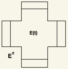
Figure 1: The evolving set $E(t)$.

We observe that Formula (17) for $E(t)$ can be easily obtained by finding explicit solutions to $(ATW)$, starting from $E_{L}=([-1,1]\times[-L,L])\cup([-L,L]\times[-1,1])$, $L>1$. A “calibration” is given by the following vector field $z$, defined in $E_{L}$:

$$z(x,y)=\begin{cases}(x,y)&\textup{ if }|x|\leq 1,|y|\leq 1,\\ (x,\pm 1)&\textup{ if }|x|\leq 1,1\leq\pm y\leq L,\\ (\pm 1,y)&\textup{ if }1\leq\pm x\leq L,|y|\leq 1.\end{cases}$$

One has $\textup{div}\,z=1+\chi_{[-1,1]^{2}}$ in $E_{L}$, $z(x,y)\in\{{\psi^{\circ}}\leq 1\}$, and $P_{\phi}(E_{\ell})=\int_{\partial E_{\ell}}z\cdot\nu\,d\mathcal{H}^{1}$ for any $1\leq\ell\leq L$. Hence, if $L-h\geq 1$ and $F\subset E_{L}$, we have

$$P_{\phi}(F)+\int_{F}\frac{d^{\psi^{\circ}}_{E_{L}}}{h}dx\geq\int_{\partial F}\nu\cdot zd\mathcal{H}^{1}+\int_{F}\frac{d^{\psi^{\circ}}_{E_{L}}}{h}dx\\ =\int_{\partial F}\nu\cdot zd\mathcal{H}^{1}-\int_{\partial E_{L-h}}\nu\cdot zd\mathcal{H}^{1}+P_{\phi}(E_{L-h})+\int_{F}\frac{d^{\psi^{\circ}}_{E_{L}}}{h}dx\\ =\int z\cdot(D\chi_{E_{L-h}}-D\chi_{F})+P_{\phi}(E_{L-h})+\int_{E_{L-h}}\frac{d^{\psi^{\circ}}_{E_{L}}}{h}dx+\int_{E_{L}}(\chi_{F}-\chi_{E_{L-h}})\frac{d^{\psi^{\circ}}_{E_{L}}}{h}dx\\ =P_{\phi}(E_{L-h})+\int_{E_{L-h}}\frac{d^{\psi^{\circ}}_{E_{L}}}{h}dx+\int_{E_{L}}(\chi_{F}-\chi_{E_{L-h}})\left(\frac{d^{\psi^{\circ}}_{E_{L}}}{h}+1+\chi_{[-1,1]^{2}}\right)dx.$$

Now, the last integral is nonnegative, since $d^{\psi^{\circ}}_{E_{L}}/h+1\leq 0$ in $E_{L-h}$, and is positive outside. As a consequence, $E_{L-h}$ solves $(ATW)$ for $E=E_{L}$, and one deduces the first line in (17). The proof of the second line in (17) is a standard computation (see for instance [7]).

4.2 Continuity of the volume up to $t=0$

We provide, in dimension $d=2$, an example of an open set $E$ satisfying $(MC_{\delta})$ for some $\delta>0$, and such that $|\partial{\{u>0\}}|>0$. The set is built as a countable union of disjoint disks.

Let $(x_{n})_{n\geq 1}$ be a dense sequence of rational points in $\Omega:=B(0,1)\subset\mathbb{R}^{2}$. We shall construct inductively a sequence $(r_{n})_{n\geq 1}$ of positive numbers with $\sum_{n}r_{n}<+\infty$ such that the following property holds: Letting $E_{0}=\emptyset$ and $E_{n}=E_{n-1}\cup B(x_{n},r_{n})$ for $n\geq 1$, the sets $E_{n}$ all satisfy $(MC_{\delta})$ in $\Omega$ for some $\delta>0$.

Notice first that there exists $\delta>0$ such that each ball $B(x,r)\subset\Omega$ satisfies $(MC_{2\delta})$ in $\Omega$. Choose now $r_{1}>0$ in such a way that $E_{1}=B(x_{1},r_{1})\subset\Omega$, then $E_{1}$ satisfies $(MC_{2\delta})$. Assume now by induction that $E_{n}$ satisfies $(MC_{(1+1/n)\delta})$. Then, if $d_{n}:=\textup{dist}(x_{n+1},E_{n})=0$ we let $r_{n+1}=0$, so that $E_{n+1}=E_{n}$. Otherwise, if $d_{n}>0$ we choose $r_{n+1}\in(0,2^{-n})$ in such a way that

$$r_{n+1}\leq\min\left(\frac{1}{2}\left(\frac{1}{n}-\frac{1}{n+1}\right)\frac{\delta d_{n}^{2}}{2\pi C},\frac{d_{n}}{6}\right),$$ (18)

where the constant $C>0$ will be chosen later in Case 3. Let also $\mathcal{N}\subset\mathbb{N}$ be the (infinite) set of indices such that $r_{n}>0$.

Assuming that $E_{n}$ satisfies $(MC_{\delta+\delta/n})$, which is true for $n=1$, Let us check that $E_{n+1}$ satisfies $(MC_{\delta(1+\delta/(n+1)})$. We consider a set $F$ of finite perimeter such that $E_{n+1}\subset F\subset\Omega$, and we distinguish three cases:

Case 1. $|F\cap B(x_{n+1},d_{n})|\geq d_{n}^{2}/C$. In this case we have

$$P(F) \geq P(E_{n})+\left(1+\frac{1}{n}\right)\delta|F\setminus E_{n}|$$

$$\geq P(E_{n+1})-2\pi r_{n+1}+\left(1+\frac{1}{n+1}\right)\delta|F\setminus E_{n}|+\left(\frac{1}{n}-\frac{1}{n+1}\right)\delta|F\cap B(x_{n+1},d_{n})|$$

$$\geq P(E_{n+1})+\left(1+\frac{1}{n+1}\right)\delta|F\setminus E_{n+1}|+\left(\frac{1}{n}-\frac{1}{n+1}\right)\frac{\delta d_{n}^{2}}{C}-2\pi r_{n+1}$$

$$\geq P(E_{n+1})+\left(1+\frac{1}{n+1}\right)\delta|F\setminus E_{n+1}|,$$

where in the last inequality we used (18).

Case 2. $|F\cap B(x_{n+1},d_{n})|\leq d_{n}^{2}/C$ and $\mathcal{H}^{1}(F\cap\partial B(x_{n+1},r))=0$ for some $r\in(r_{n+1},d_{n})$. In this case, we write $F=F_{1}\cup F_{2}$, with $F_{1}=F\cap B(x_{n+1},r)\supset B(x_{n+1},r_{n+1})$ and $F_{2}=F\setminus B(x_{n+1},r)\supset E_{n}$, and we have

$$P(F_{1}) \geq P(B(x_{n+1},r_{n+1}))+2\delta|F_{1}\setminus B(x_{n+1},r_{n+1})|$$

$$P(F_{2}) \geq P(E_{n})+\left(1+\frac{1}{n}\right)\delta|F_{2}\setminus E_{n}|.$$

Summing up the two inequalities above, we get

$$P(F) = P(F_{1})+P(F_{2})\ \geq\ P(E_{n+1})+\left(1+\frac{1}{n}\right)\delta\left(|F_{1}\setminus B(x_{n+1},r_{n+1})|+|F_{2}\setminus E_{n}|\right)$$

$$= P(E_{n+1})+\left(1+\frac{1}{n}\right)\delta|F\setminus E_{n+1}|.$$

Case 3. $|F\cap B(x_{n+1},d_{n})|\leq d_{n}^{2}/C$ and $\mathcal{H}^{1}(F\cap\partial B(x_{n+1},r))>0$ for a.e. $r\in(r_{n+1},d_{n})$. In this case, by co-area formula we have

$$\int_{\frac{d_{n}}{6}}^{\frac{d_{n}}{3}}\mathcal{H}^{1}(F\cap\partial B(x_{n+1},r))\,dr=\left|F\cap\left(B\left(x_{n+1},\frac{d_{n}}{3}\right)\setminus B\left(x_{n+1},\frac{d_{n}}{6}\right)\right)\right|\leq\frac{d_{n}^{2}}{C}.$$

It follows that there exists $\rho_{1}\in(d_{n}/6,d_{n}/3)$ such that

$$\mathcal{H}^{1}(F\cap\partial B(x_{n+1},\rho_{1}))\leq\frac{6d_{n}}{C}.$$

Similarly we have

$$\int_{\frac{2d_{n}}{3}}^{d_{n}}\mathcal{H}^{1}(F\cap\partial B(x_{n+1},r))\,dr=\left|F\cap\left(B(x_{n+1},d_{n})\setminus B\left(x_{n+1},\frac{2d_{n}}{3}\right)\right)\right|\leq\frac{d_{n}^{2}}{C},$$

and there exists $\rho_{2}\in(2d_{n}/3,d_{n})$ such that

$$\mathcal{H}^{1}(F\cap\partial B(x_{n+1},\rho_{2}))\leq\frac{3d_{n}}{C}.$$

Using that $\mathcal{H}^{1}(F\cap\partial B(x_{n+1},r))>0$ for all $r\in(r_{n+1},d_{n})$ we deduce that

• either for a.e. $r\in(\rho_{1},\rho_{2})$, it holds $\mathcal{H}^{0}(\partial^{*}F\cap\partial B(x_{n+1},r))\geq 2$, and it follows that $P(F,B(x_{n+1},\rho_{2})\setminus B(x_{n+1},\rho_{1}))\geq 2(\rho_{2}-\rho_{1})\geq 2d_{n}/3$,

• or for a set of positive measure of radii $r\in(\rho_{1},\rho_{2})$ one has $\mathcal{H}^{1}(F\cap\partial B(x_{n+1},r))=2\pi r$. In this case, observe that for a.e. $y\in\partial B(x_{n+1},\rho_{1})\setminus F$, the ray from $x_{n+1}$ to $\partial B(x_{n+1},r)$ through $y$ crosses $\partial^{*}F$ at least once outside of $\overline{B}(x_{n+1},\rho_{1})$ so that the projection of $\partial^{*}F\cap B(x_{n+1},\rho_{2})\setminus B(x_{n+1},\rho_{1})$ onto $\partial B(x_{n+1},\rho_{1})$ has measure at least $2\pi\rho_{1}-6d_{n}/C$. Hence,

  $$P(F,B(x_{n+1},\rho_{2})\setminus B(x_{n+1},\rho_{1}))\geq 2\pi\rho_{1}-6d_{n}/C\\ \geq d_{n}(\pi/3-6/C)\geq 2d_{n}/3$$

  provided we have chosen $C\geq 18/(\pi-2)$.

Then, proceeding as in the previous case we let $F_{1}=F\cap B(x_{n+1},\rho_{1})$ and $F_{2}=F\setminus B(x_{n+1},\rho_{2})$, and we have

$$P(F)= \ P(F_{1})+P(F_{2})-\mathcal{H}^{1}(F\cap\partial B(x_{n+1},\rho_{1}))-\mathcal{H}^{1}(F\cap\partial B(x_{n+1},\rho_{2}))$$

$$\hskip 176.407pt+\ P(F,B(x_{n+1},\rho_{2})\setminus B(x_{n+1},\rho_{1}))$$

$$\geq \ P(E_{n+1})+\left(1+\frac{1}{n}\right)\delta\left(|F_{1}\setminus B(x_{n+1},r_{n+1})|+|F_{2}\setminus E_{n}|\right)-\frac{9d_{n}}{C}+\frac{2d_{n}}{3}$$

$$\geq \ P(E_{n+1})+\left(1+\frac{1}{n}\right)\delta|F\setminus E_{n+1}|-\left(1+\frac{1}{n}\right)\delta\frac{d_{n}^{2}}{C}-\frac{9d_{n}}{C}+\frac{2d_{n}}{3}$$

$$\geq \ P(E_{n+1})+\left(1+\frac{1}{n}\right)\delta|F\setminus E_{n+1}|-\frac{2\delta+9}{C}d_{n}+\frac{2d_{n}}{3}$$

$$\geq \ P(E_{n+1})+\left(1+\frac{1}{n}\right)\delta|F\setminus E_{n+1}|,$$

as long as we choose $C\geq 3(2\delta+9)/2$.

We proved that $E_{n}$ satisfies $(MC_{\delta})$ for all $n\in\mathcal{N}$, therefore also the limit set

$$E:=\bigcup_{n\in\mathcal{N}}E_{n}=\bigcup_{n\in\mathcal{N}}B(x_{n},r_{n})$$

satisfies $(MC_{\delta})$ in $\Omega$. In this case, the solution $u$ in Theorem 3.1 is explicit and it is given by

$$u(x)=\sum_{n\in\mathcal{N}}\frac{(r_{n}^{2}-|x-x_{n}|^{2})^{+}}{2}.$$

Notice that we have

$$\partial\{u>0\}=\partial E=\overline{B(0,1)}\setminus E,$$

so that $|\partial\{u>0\}|=\pi-|E|>0$.

Appendix A $\mathbf{1}$-superharmonic functions

The goal of this appendix is to recall some results proved in [22] on $1$-superharmonic functions, to give precise statements in the anisotropic case, and to propose some simple proofs, when possible.

Definition A.1.

We say that $u$ is ($\phi$-)$1$-superharmonic in $\Omega$ if $\{u\neq 0\}\subset\subset\Omega$ and for any $v$ with $v\geq u$, $\{v\neq 0\}\subset\subset\Omega$, one has

$$\int_{\Omega}\phi(-Du)\leq\int_{\Omega}\phi(-Dv),$$

or, equivalently, for any $v$ with compact support in $\Omega$,

$$\int_{\Omega}\phi(-D(u\wedge v))\leq\int_{\Omega}\phi(-Dv).$$

Given $\delta>0$, we say that $u$ is ($(\phi,\delta)$-)$1$-superharmonic in $\Omega$ if $\{u\neq 0\}\subset\subset\Omega$ and one has:

$$\int_{\Omega}\phi(-D(u\wedge v))\leq\int_{\Omega}\phi(-Dv)-\delta\int_{\Omega}(v-u)^{+}dx\quad\forall\ v,\{v\neq 0\}\subset\subset\Omega.$$

Equivalently, $u$ is a minimizer of

$$\int_{\Omega}\phi(-Du)-\delta\int_{\Omega}udx,$$

with respect to larger competitors with the same boundary condition.

Obviously then, $u\geq 0$ (using $v=u^{+}$ in $(SH)$). Notice that $\chi_{E}$ is $1$-superharmonic if and only if the set $E$ is outward minimizing.

Observe that, in this case, the set $E^{0}=\{u>0\}$ has finite perimeter and satisfies $(MC_{\delta})$. Indeed, for $E\subset F\subset\subset\Omega$, letting $v=\varepsilon\chi_{F}$ for $\varepsilon>0$, we have

$$\int_{\Omega}\phi(-D(u\wedge\varepsilon\chi_{F}))=\int_{0}^{\varepsilon}P_{\phi}(\{u>s\}\cap F)ds\\ \leq\varepsilon P_{\phi}(F)-\delta\int_{\Omega}(\varepsilon\chi_{F}-u)^{+}dx=\varepsilon\left(P_{\phi}(F)-\delta\int_{\Omega}(\chi_{F}-u/\varepsilon)^{+}dx\right).$$

Hence:

$$\int_{0}^{1}P_{\phi}(\{u>t\varepsilon\}\cap F)dt\leq P_{\phi}(F)-\delta\int_{\Omega}(\chi_{F}-u/\varepsilon)^{+}dx.$$

Sending $\varepsilon\to 0$, we deduce $(MC_{\delta})$.

In particular, it follows from Lemma 2.6 that for any $v\in BV(\Omega)$ compactly supported, $\delta\int_{\Omega}|v|dx\leq\int_{\Omega}\phi(-Dv)$. We then deduce that if $u$ satisfies $(SH_{\delta})$ also $u\wedge T$ for any $T>0$. Indeed,

$$\int_{\Omega}\phi(-D((u\wedge T)\wedge v))\leq\int_{\Omega}\phi(-D(v\wedge T))-\delta\int_{\Omega}((v\wedge T)-u)^{+}dx$$

On the other hand,

$$\int_{\Omega}\phi(-D(v\wedge T))=\int_{\Omega}\phi(-Dv)-\int_{\Omega}\phi(-D(v-T)^{+})\leq\int_{\Omega}\phi(-Dv)-\delta\int_{\Omega}(v-T)^{+}\,dx,$$

and it follows

$$\int_{\Omega}\phi(-D((u\wedge T)\wedge v))\leq\int_{\Omega}\phi(-Dv)-\delta\int_{\Omega}(v-(u\wedge T))^{+}dx.$$

Then, the following characterization holds:

Proposition A.2.

Let $u$ satisfy $(SH_{\delta})$. Then there exists $z\in L^{\infty}(\Omega;\{{\phi^{\circ}}\leq 1\})$ with $\textup{div}\,z\geq\delta$, $[z,Du^{+}]=|Du|$ in the sense of measures (equivalently, $\int_{\Omega}u^{+}\textup{div}\,z\,dx=\int\phi(-Du)$), and $\textup{div}\,z=\delta$ on $\{u=0\}$.

Corollary A.3.

Let $u$ satisfy $(SH_{\delta})$. Then for any $s>0$, $\{u^{+}\geq s\}$ and $\{u^{+}>s\}$ satisfy $(MC_{\delta})$.

Here, $u^{+}$ is as usual the superior approximate limit of $u$ (defined $\mathcal{H}^{d-1}$-a.e.) and $[z,Du^{+}]$ the pairing in the sense of Anzellotti [6].

Proof.

For $n\geq 1$, let $v_{n}$ be the unique minimizer of

$$\min_{v=0\ \partial\Omega}\int_{\Omega}\phi(-Dv)+\int_{\Omega}\frac{n}{2}(v-u\wedge n)^{2}-\delta v\,dx.$$ (19)

(the boundary condition is to be intended in a relaxed sense, adding a term $\int_{\partial\Omega}|\textup{Tr}v|\phi(\nu_{\Omega})d\mathcal{H}^{d-1}$ in the energy if the trace of $v$ on the boundary does not vanish). The Euler-Lagrange equation for this problem asserts the existence of a field $z_{n}\in L^{\infty}(\Omega;\{{\phi^{\circ}}\leq 1\})$ with bounded divergence such that

$$\textup{div}\,z_{n}+nv_{n}=n(u\wedge n)+\delta$$

a.e. in $\Omega$, and $\int_{\Omega}\textup{div}\,z_{n}v_{n}\,dx=\int_{\Omega}\phi(-Dv_{n})$. On the other hand $\int_{\Omega}\phi(-Dv_{n})\leq\int_{\Omega}\phi(-D(u\wedge n))\leq\int_{\Omega}\phi(-Du)$ and we have $v_{n}\to u$, $\int_{\Omega}\phi(-Dv_{n})\to\int_{\Omega}\phi(-Du)$ as $n\to\infty$.

We show that $v_{n}\leq u\wedge n$. Indeed, $\int_{\Omega}\phi(-D(v_{n}\wedge u\wedge n))\leq\int_{\Omega}\phi(-Dv_{n})-\delta\int_{\Omega}(v_{n}-(u\wedge n))^{+}dx$, while $\int_{\Omega}(v_{n}-(u\wedge n))^{2}dx\geq\int_{\Omega}((v_{n}\wedge u\wedge n)-(u\wedge n))^{2}$. Hence,

$$\int_{\Omega}\phi(-D(v_{n}\wedge u\wedge n))+\frac{n}{2}\int_{\Omega}((v_{n}\wedge u\wedge n)-(u\wedge n))^{2}-\delta\int_{\Omega}(v_{n}\wedge u\wedge n)dx\\ \leq\int_{\Omega}\phi(-Dv_{n})+\frac{n}{2}\int_{\Omega}(v_{n}-(u\wedge n))^{2}dx-\delta\int_{\Omega}v_{n}dx\\ +\delta\int_{\Omega}(v_{n}-(v_{n}\wedge u\wedge n))-(v_{n}-(u\wedge n))^{+}dx\\ =\int_{\Omega}\phi(-Dv_{n})+\frac{n}{2}\int_{\Omega}(v_{n}-(u\wedge n))^{2}dx-\delta\int_{\Omega}v_{n}dx$$

and as the minimizer $v_{n}$ of (19) is unique, we deduce $v_{n}=v_{n}\wedge u\wedge n$. In particular, it follows $\textup{div}\,z_{n}\geq\delta$. (Observe that since $v_{n}\geq 0$, one also has $\textup{div}\,z_{n}\leq\delta+n(u\wedge n)$, in particular $\textup{div}\,z_{n}=\delta$ a.e. in $\{u=0\}$. Also, $\int_{\{u>0\}}\textup{div}\,z_{n}\leq P_{\phi}(E^{0})$, hence $(\textup{div}\,z_{n})_{n\geq 1}$ are uniformly bounded Radon measures. Hence, up to a subsequence, we may assume that $z_{n}\stackrel{{\scriptstyle*}}{{\rightharpoonup}}z$ weakly-$*$ in $L^{\infty}(\Omega;\{{\phi^{\circ}}\leq 1\})$ while $\textup{div}\,z_{n}\stackrel{{\scriptstyle*}}{{\rightharpoonup}}\textup{div}\,z$ weakly-$*$ in $\mathcal{M}^{1}(\Omega;\mathbb{R}_{+})$, that is, as positive measures.

We now write

$$\int_{\Omega}\phi(-Dv_{n})=\int_{\Omega}v_{n}\textup{div}\,z_{n}\,dx\leq\int_{\Omega}(u\wedge n)\textup{div}\,z_{n}\,dx=\int_{0}^{n}\int_{\{u\geq s\}}\textup{div}\,z_{n}\,dxds,$$

hence, since $v_{n}\to u$,

$$\int_{\Omega}\phi(-Du)\leq\limsup_{n\to\infty}\int_{0}^{n}\int_{\{u\geq s\}}\textup{div}\,z_{n}\,dxds\leq\int_{0}^{\infty}\left(\limsup_{n\to\infty}\int_{\{u\geq s\}}\textup{div}\,z_{n}\,dx\right)ds$$

thanks to Fatou’s lemma (and the fact $\int_{\{u\geq s\}}\textup{div}\,z_{n}\,dx\leq P_{\phi}(E^{0})$ are uniformly bounded).

We now study the limit of $\int_{\{u\geq s\}}\textup{div}\,z_{n}\,dx$, for $s>0$ given, assuming $\{u>s\}$ has finite perimeter (this is true for a.e. $s$, and in fact one could independently check that $s\mapsto P_{\phi}(\{u\geq s\})$ is nonincreasing).

We consider a set $F=\{u\geq s\}$ with finite perimeter, and we recall $D\chi_{F}$ is supported on the reduced boundary $\partial^{*}F$. By inner regularity, given $\varepsilon>0$, we find a compact set $K\subset\partial^{*}F$ with $|D\chi_{F}|(\Omega\setminus K)<\varepsilon$. We observe that $\mathcal{H}^{d-1}$-a.e. on $K$ (which is countably rectifiable), $\chi_{F}$ has an upper an lower trace, respectively $\chi_{F}^{+}=1$ and $\chi_{F}^{-}=0$. By the Meyers-Serrin Theorem (or its $BV$ version, cf [5] or [4, Theorem 3.9]), there exists $\varphi_{k}$ a sequence of functions in $C^{\infty}(\Omega\setminus K;[0,1])$ with $\varphi_{k}\to\chi_{F}$ and

$$\int_{0}^{1}\mathcal{H}^{d-1}(\{x\in\Omega\setminus K:\varphi_{k}(x)=k\})=\int_{\Omega\setminus K}|\nabla\varphi_{k}|dx\to|D\chi_{F}|(\Omega\setminus K)<\varepsilon.$$

Moreover, by construction the traces of $\varphi_{k}$ in $K$ coincide with the traces of $\chi_{F}$ (see [4, Section 3.8]).

We choose for each $k$ $s_{k}\in[1/4,3/4]$ such that $\mathcal{H}^{d-1}(\partial\{\varphi_{k}\geq s_{k}\}\setminus K)\leq 2\varepsilon$. We then define the closed (compact) sets $F_{k}:=\{\varphi_{k}\geq s_{k}\}\cup K$. One has $\int_{\Omega}|D\chi_{F}-D\chi_{F_{k}}|=\int_{\Omega\setminus K}|D\chi_{F}-D\chi_{F_{k}}|\leq 3\varepsilon$. (This shows that $F$ can be approximated strongly in $BV$ norm by closed sets.)

Then, one has $\limsup_{n}\int_{F_{k}}\textup{div}\,z_{n}dx\leq\int_{F_{k}}\textup{div}\,z$ as the measures are nonnegative and $\chi_{F_{k}}$ is scs. On the other hand, $|\int_{\Omega}\textup{div}\,z_{n}(\chi_{F}-\chi_{F_{k}})dx|\leq 3\varepsilon$, so that

$$\limsup_{n\to\infty}\int_{F}\textup{div}\,z_{n}dx\leq 3\varepsilon+\int_{F}\textup{div}\,z+\int(\chi_{F_{k}}-\chi_{F})\textup{div}\,z\leq 3\varepsilon+\int_{F}\textup{div}\,z+\int(\chi_{F_{k}}-\chi_{F})^{+}\textup{div}\,z.$$

Notice that it is important to specify precisely the set $F$ that we consider in the last inequality: We pick for $F$ the complement $F^{+}$ of its points of density zero, equivalently $F^{+}=\{u^{+}\geq s\}$. In that case, up to a set of zero $\mathcal{H}^{d-1}$-measure, $\chi_{G}:=(\chi_{F_{k}}-\chi_{F^{+}})^{+}=\chi_{F_{k}\setminus F^{+}}$ vanishes on $K$ pointwise, moreover at $\mathcal{H}^{d-1}$-a.e. $x\in K$, $G$ has Lebesgue density $0$. Hence $G$ coincides $\mathcal{H}^{d-1}$-a.e. with a Caccioppoli set strictly inside $\Omega$ and with $\int_{\Omega}|D\chi_{G}|\leq 3\varepsilon$. Thanks to [24, Thm 5.12.4] it follows $\textup{div}\,z(G)\leq C\varepsilon$ for $C$ depending only on $\phi$ and the dimension (see also [22, Prop. 3.5]). As a consequence, since $\varepsilon>0$ is arbitrary,

$$\limsup_{n\to\infty}\int_{\{u\geq s\}}\textup{div}\,z_{n}dx\leq\int_{\{u^{+}\geq s\}}\textup{div}\,z.$$

We obtain that

$$\int_{\Omega}\phi(-Du)\leq\int_{\Omega}u^{+}\textup{div}\,z.$$

The reverse inequality also holds thanks to [22, Prop. 3.5, (3.9)], and can be proved by localizing and smoothing with kernels depending on the local orientation of the jump. We also deduce that, for a.e. $s>0$,

$$\int_{\{u^{+}\geq s\}}\textup{div}\,z=P_{\phi}(\{u\geq s\})\,.$$

Note that $s\mapsto\textup{div}\,z({\{u^{+}\geq s\}})$ is left-continuous, and $s\mapsto\textup{div}\,z({\{u^{+}>s\}})$ is right-continuous, whereas $s\mapsto P_{\phi}(\{u^{+}\geq s\})$ is left-semicontinuous, which implies the thesis. ∎

References

- [1] L. Almeida, A. Chambolle, and M. Novaga. Mean curvature flow with obstacles. Ann. Inst. H. Poincaré Anal. Non Linéaire, 29(5):667–681, 2012.
- [2] Fred Almgren, Richard Schoen, and Leon Simon. Regularity and singularity estimates of hypersurfaces minimizing parametric elliptic variational integrals. Acta Math., 139:217–265, 1977.
- [3] Fred Almgren, Jean Taylor, and Lihe Wang. Curvature-driven flows: a variational approach. SIAM J. Control Optim., 31(2):387–438, 1993.
- [4] Luigi Ambrosio, Nicola Fusco, and Diego Pallara. Functions of bounded variation and free discontinuity problems. Oxford Mathematical Monographs. Oxford University Press, New York, 2000.
- [5] Gabriele Anzellotti and Mariano Giaquinta. BV functions and traces. Rend. Sem. Mat. Univ. Padova, 60:1–21, 1978.
- [6] Gabriele Anzellotti. Pairings between measures and bounded functions and compensated compactness. Ann. Mat. Pura Appl. (4), 135:293–318, 1983.
- [7] Giovanni Bellettini, Vicent Caselles, Antonin Chambolle, and Matteo Novaga. Crystalline mean curvature flow of convex sets. Arch. Ration. Mech. Anal., 179(1):109–152, 2006.
- [8] J. W. Cahn and D. W. Hoffmann. A vector thermodynamics for anisotropic surfaces-ii. curved and faceted surfaces. Acta Metallurgica, 22:1205–1214, 1974.
- [9] David G. Caraballo. Flat curvature flow of convex sets. Taiwanese J. Math., 16(1):1–12, 2012.
- [10] Vicent Caselles, Gabriele Facciolo, and Enric Meinhardt. Anisotropic Cheeger sets and applications. SIAM J. Imaging Sci., 2(4):1211–1254, 2009.
- [11] Vicent Caselles and Antonin Chambolle. Anisotropic curvature-driven flow of convex sets. Nonlinear Anal., 65(8):1547–1577, 2006.
- [12] Antonin Chambolle, Massimiliano Morini, Matteo Novaga, and Marcello Ponsiglione. Existence and uniqueness for anisotropic and crystalline mean curvature flows. Jour. Amer. Math. Soc., 32(3):779–824, 2019.
- [13] Antonin Chambolle, Massimiliano Morini, Matteo Novaga, and Marcello Ponsiglione. Generalized crystalline evolutions as limits of flows with smooth anisotropies. Anal. PDE, 12(3):789–813, 2019.
- [14] Antonin Chambolle, Massimiliano Morini, and Marcello Ponsiglione. Existence and uniqueness for a crystalline mean curvature flow. Comm. Pure Appl. Math., 70(6):1084–1114, 2017.
- [15] Guido De Philippis and Tim Laux. Implicit time discretization for the mean curvature flow of mean convex sets. arXiv:1806.02716, to appear on Ann. Sc. Norm. Sup. Pisa Cl. Sci.
- [16] Alessio Figalli. Regularity of codimension-1 minimizing currents under minimal assumptions on the integrand. J. Differential Geom., 106(3):371–391, 2017.
- [17] M.-H. Giga and Y. Giga. Generalized motion by nonlocal curvature in the plane. Arch. Ration. Mech. Anal., 159(4):295–333, 2001.
- [18] Stephan Luckhaus and Thomas Sturzenhecker. Implicit time discretization for the mean curvature flow equation. Calc. Var. Partial Differential Equations, 3(2):253–271, 1995.
- [19] Alessandra Lunardi. Analytic semigroups and optimal regularity in parabolic problems. Modern Birkhäuser Classics. Birkhäuser/Springer Basel AG, Basel, 1995.
- [20] Francesco Maggi. Sets of finite perimeter and geometric variational problems. An introduction to geometric measure theory. Cambridge Studies in Advanced Mathematics, 135. Cambridge University Press, Cambridge, 2012.
- [21] Jan Metzger and Felix Schulze. No mass drop for mean curvature flow of mean convex hypersurfaces. Duke Math. J., 142(2):283–312, 2008.
- [22] Christoph Scheven and Thomas Schmidt. BV supersolutions to equations of 1-Laplace and minimal surface type. J. Differential Equations, 261(3):1904–1932, 2016.
- [23] Leon Simon. On Some Extensions of Bernstein’s Theorem. Math. Z., 154:265–273, 1977.
- [24] William P. Ziemer. Weakly differentiable functions. Graduate Texts in Mathematics, 120. Springer-Verlag, New York, 1989.