Analyses of residual accelerations for TianQin based on the global MHD simulation

Abstract

TianQin is a proposed space-based gravitational wave observatory. It is designed to detect the gravitational wave signals in the frequency range of 0.1 mHz – 1 Hz. At a geocentric distance of $10^{5}$ km, the plasma in the earth magnetosphere will contribute as the main source of environmental noises. Here, we analyze the acceleration noises that are caused by the magnetic field of space plasma for the test mass of TianQin. The real solar wind data observed by the Advanced Composition Explorer are taken as the input of the magnetohydrodynamic simulation. The Space Weather Modeling Framework is used to simulate the global magnetosphere of the earth, from which we obtain the plasma and magnetic field parameters on the detector’s orbits at $\varphi_{s}$ = $0^{\circ}$, $30^{\circ}$, $60^{\circ}$ and $90^{\circ}$, where $\varphi_{s}$ is the acute angle between the line that joins the sun and the earth and the projection of the normal of the detector’s plane on the ecliptic plane. We calculate the time series of the residual accelerations and the corresponding amplitude spectral densities on these orbit configurations. We find that the residual acceleration produced by the interaction between the TM’s magnetic moment induced by the space magnetic field and the spacecraft magnetic field ($\bm{a}_{\rm M1}$) is the dominant term, which can approach $10^{-15}$ m/s²/Hz^1/2 at $f\approx$ 0.2 mHz for the nominal values of the magnetic susceptibility ($\chi_{\rm m}=10^{-5}$) and the magnetic shielding factor ($\xi_{\rm m}=10$) of the test mass. The ratios between the amplitude spectral density of the acceleration noise caused by the space magnetic field and the preliminary goal of the inertial sensor are 0.38 and 0.08 at 1 mHz and 10 mHz, respectively. We discuss the further reduction of this acceleration noise by decreasing $\chi_{\rm m}$ and/or increasing $\xi_{\rm m}$ in the future instrumentation development for TianQin.

Keywords: gravitational waves, space plasma, test mass, acceleration noise

1 Introduction

Since the direct detection of the gravitational waves (GWs) from the merger of a pair of stellar mass black holes (GW150914) by the two advanced detectors of the Laser Interferometer Gravitational-Wave Observatory (LIGO) [1], more than ten GW events have been detected by advanced LIGO and advanced Virgo [2, 3, 4, 5, 6, 7]. Recently, KAGRA [8] has joined the ground-based GW detector network. Due to the unshieldable impacts from the environment, namely seismic noise and gravity gradient noise, it is very difficult for these terrestrial laser interferometers to detect GWs with the frequencies lower than 10 Hz. However, in the low frequencies, there are rich sources of GWs that can be used to study the fundamental physics, astrophysics and cosmology [9]. The aim of space-borne laser interferometers is to explore the GWs in the millihertz range (0.1 mHz–1 Hz). Several projects, e.g., LISA [10], TianQin (TQ) [11], DECIGO [12], ASTROD-GW [13], g-LISA [14], Taiji (ALIA descoped) [15] and BBO [16] have been proposed and are currently under different stages of study and development.

Both LISA and TQ have three drag-free spacecraft which compose a nearly equilateral triangular constellation. Different from LISA, TQ’s spacecraft will be deployed in a geocentric orbit with an altitude of $1\times 10^{5}$ km from the geocenter, which makes the distances between each pair of spacecraft $\approx$ $1.7\times 10^{5}$ km [11]. The normal of the detector’s plane formed by the three spacecraft points toward the candidate ultracompact white-dwarf binary RX J0806.3+1527 [17]. The three spacecraft are interconnected by infrared laser beams and form up to three Michelson-type interferometers. The heterodyne transponder-type laser interferometers are used to measure the displacements of the test masses (TMs) to the accuracy of $10^{-12}~{}\rm{m/Hz^{1/2}}$ in millihertz. The disturbance reduction system is designed to reduce the non-conservative acceleration of each TM (Pt-Au alloy, $m=2.45~{}\rm{kg}$) down to $10^{-15}~{}\rm{m/s^{2}/Hz^{1/2}}$ in millihertz [11]. The nominal orbit and a set of alternatives for TQ have been optimized such that the stability of the orbits, in terms of the variations of arm lengths, breathing angles and relative range rates, can meet the requirements imposed by the long range space laser interferometry [18]. The response of TQ as a Michelson interferometer and its sensitivity curve have been given [19]. Its science objectives involving astrophysical sources [20, 21, 22, 23] and cosmological sources [24, 25] are currently under intensive investigations.

In space, the space plasma will serve as the main source of environmental noises. One example is the dispersion effect induced by the space plasma when the laser beams propagate from one spacecraft to the other [26]. It can cause time-varying optical paths and time delays, hence affects the displacement measurement accuracy. Taking the typical magnitudes of electron number density and magnetic field in the earth magnetosphere as 1–10 cm^-3 and 1–10 nT [27, 28], respectively, at the altitude of TQ’s spacecraft, one can see that the dominating factor of the dispersion is from the former.

On the other hand, the magnetic field plays a central role in the formation of the structures in heliophysics, such as the photosphere and corona of the Sun [29, 30], Parker spiral field lines [31], the boundary of the heliosphere [32], and the magnetosphere of the Earth, Jupiter and Saturn [33, 34]. For LISA, it has been shown that the magnetic field of space plasma is the main source of the non-conservative forces acting on the TMs housed in the spacecraft through the interactions with its magnetic remanence and residual charges [35, 36]. Evaluating the impacts of these residual accelerations for TQ is the focus of this work.

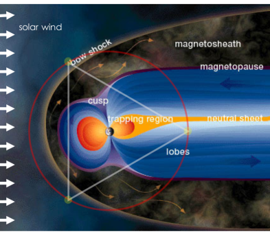
Figure 1: The schematic view of TQ’s orbit (red circle) in the background of the global magnetosphere at $\varphi_{s}\approx 90^{\circ}$. Thin white lines are the laser beams that interconnect the spacecraft of TQ (filled yellow circles). Modified from [83].

In Fig. 1, TQ’s orbit (red circle) will pass through different background environments, including solar wind, bow shock, magnetosheath, magnetopause, lobes of magnetosphere, magnetotail and so on. There are abundant phenomena of space plasma at this orbit altitude, which cover three spatial scales: the global scale, the magnetohydrodynamic (MHD) scale and the plasma scale. In the global scale, the earth magnetosphere is formed by the interaction between the solar wind and the magnetosphere. The variations of the parameters (e.g., velocity, magnetic field) in solar wind can change the shape and position of the bow shock and the magnetopause [37]. In the MHD scale, there are instabilities, such as Kelvin-Helmholtz instability at the magnetopause [38]. In the plasma scale, the turbulance in solar wind and magnetosheath [39, 40, 27] and the plasma waves in solar wind and magnetosphere [41, 42, 43] are ubiquitous. Besides, the disturbances from the sun (e.g., coronal mass ejections, coronal shocks [44, 45, 46]) and the magnetosphere (e.g., magnetic storms, magnetic reconnections [47, 48, 49]) take place occasionally. All these phenomena can lead to the variations of the electron number density and the magnetic field, which in turn lead to the fluctuations of the dispersion along the optical paths and the non-conservative forces on the TMs.

The rest of the paper is organized as follows. Section 2 gives the formalism that is subsequently used to analyze the acceleration noises of TMs induced by the magnetic field of the space plasma. In section 3, we use a well established MHD model (Space Weather Modeling Framework; SWMF [50]) to simulate a magnetospheric environment that TQ’s spacecraft may encounter. The inclinations of TQ detector’s plane in the magnetosphere ($\varphi_{s}$) are discussed. In section 4, based on the simulated magnetic field, we calculate the acceleration noises and the associated amplitude spectral densities (ASDs) at four typical values of $\varphi_{s}$, and discuss its reduction in the parameter space of $\xi_{\rm m}-\chi_{\rm m}$. The paper is concluded in section 5.

2 Acceleration noise analysis

In the magnetic field of space plasma, there are two kinds of non-conservative forces acting on the TMs. The first one is the magnetic force produced by the interaction between the TM with a magnetic moment and the background magnetic field. The second one is the Lorentz force that produced by the movement of the TM with residual charges in this magnetic field.

2.1 Magnetic force

The magnetic force on the TM with a magnetic moment ($\bm{M}_{\rm tm}$) in the background magnetic field ($\bm{B}$) can be written as:

$$\bm{F}=\nabla(\bm{M}_{\rm tm}\cdot\bm{B})\,.$$ (1)

Here, $\bm{B}$ is composed of the space magnetic field $\bm{B}_{\rm sp}$ and the spacecraft magnetic field $\bm{B}_{\rm sc}$ inherited from the payloads (e.g., permanent magnet used in attitude control or laser frequency stabilization), i.e., $\bm{B}=\bm{B}_{\rm sp}+\bm{B}_{\rm sc}$. $\bm{M}_{\rm tm}$ is composed of the remanent magnetic moment $\bm{M}_{\rm r}$ and the inductive magnetic moment $\bm{M}_{\rm i}$: $\bm{M}_{\rm tm}=\bm{M}_{\rm r}+\bm{M}_{\rm i}$. $\bm{M}_{\rm i}$ can be induced both by $\bm{B}_{\rm sp}$ and $\bm{B}_{\rm sc}$,

$$\bm{M}_{\rm i}=\frac{\chi_{\rm m}V_{\rm tm}(\bm{B}_{\rm sp}+\bm{B}_{\rm sc})}{\mu_{0}}=\bm{M}_{\rm isp}+\bm{M}_{\rm isc}\,,$$ (2)

where, $\mu_{0}$ is the vacuum magnetic permeability, $\chi_{\rm m}$ is the magnetic susceptibility, and $V_{\rm tm}$ is the volume of the TM. Inserting $\bm{M}_{\rm tm}$ and Equation (2) into Equation (1), the acceleration can be expressed as follows:

$$\begin{split}\bm{a}_{\rm M}&=\frac{1}{m}\nabla[(\bm{M}_{\rm r}+\bm{M}_{\rm isp}+\bm{M}_{\rm isc})\cdot(\bm{B}_{\rm sp}+\bm{B}_{\rm sc})]\\ &=\frac{1}{m}\nabla(\bm{M}_{\rm r}\cdot\bm{B}_{\rm sp}+\bm{M}_{\rm r}\cdot\bm{B}_{\rm sc}+\frac{\chi_{\rm m}V_{\rm tm}}{\mu_{0}}B_{\rm sp}^{2}+\frac{2\chi_{\rm m}V_{\rm tm}}{\mu_{0}}\bm{B}_{\rm sp}\cdot\bm{B}_{\rm sc}+\frac{\chi_{\rm m}V_{\rm tm}}{\mu_{0}}B_{\rm sc}^{2})\,,\end{split}$$ (3)

where $m$ is the mass of the TM, $B_{\rm sc}=|\bm{B}_{\rm sc}|$, $B_{\rm sp}=|\bm{B}_{\rm sp}|$. Based on the vector operation rules, the first term in the second line of Equation (3) can be expanded as:

$$\nabla(\bm{M}_{\rm r}\cdot\bm{B}_{\rm sp})=(\bm{M}_{\rm r}\cdot\nabla)\bm{B}_{\rm sp}+(\bm{B}_{\rm sp}\cdot\nabla)\bm{M}_{\rm r}+\bm{M}_{\rm r}\times(\nabla\times\bm{B}_{\rm sp})+\bm{B}_{\rm sp}\times(\nabla\times\bm{M}_{\rm r})\,.$$ (4)

According to Maxwell Equations, $\nabla\times\bm{B}$ can be induced by the electric current density $\bm{j}$ and the displacement current density $\varepsilon_{0}\partial\bm{E}/\partial t$, where $\varepsilon_{0}$ is the vacuum electric permittivity. Since the TM is encapsulated by the house of the inertial sensor in the disturbance reduction system, the electric current on the TM can be ignored. Therefore, Equation (4) can be written as:

$$\nabla(\bm{M}_{\rm r}\cdot\bm{B}_{\rm sp})=(\bm{M}_{\rm r}\cdot\nabla)\bm{B}_{\rm sp}+(\bm{B}_{\rm sp}\cdot\nabla)\bm{M}_{\rm r}+\bm{M}_{\rm r}\times(\frac{\varepsilon_{0}\mu_{0}\partial\bm{E}_{\rm sp}}{\partial t})+\bm{B}_{\rm sp}\times(\nabla\times\bm{M}_{\rm r})\,.$$ (5)

Similarly, the second term in Equation (3) can be expanded as Equation (5) with $\bm{B}_{\rm sp}$ and $\bm{E}_{\rm sp}$ replaced by $\bm{B}_{\rm sc}$ and $\bm{E}_{\rm sc}$. And the forth term in Equation (3) can be expanded as:

$$\nabla(\bm{B}_{\rm sp}\cdot\bm{B}_{\rm sc})=(\bm{B}_{\rm sp}\cdot\nabla)\bm{B}_{\rm sc}+(\bm{B}_{\rm sc}\cdot\nabla)\bm{B}_{\rm sp}+\bm{B}_{\rm sp}\times(\frac{\varepsilon_{0}\mu_{0}\partial\bm{E}_{\rm sc}}{\partial t})+\bm{B}_{\rm sc}\times(\frac{\varepsilon_{0}\mu_{0}\partial\bm{E}_{\rm sp}}{\partial t})\,.$$ (6)

According to $\nabla(uv)=u\nabla v+v\nabla u$, where $v$ and $u$ are scalars, the third and fifth term in Equation (3) can be written as:

$$\nabla(B_{\rm sp}^{2})=2B_{\rm sp}\nabla B_{\rm sp}\,,$$ (7)

$$\nabla(B_{\rm sc}^{2})=2B_{\rm sc}\nabla B_{\rm sc}\,.$$ (8)

Insert Equations (5)–(8) into Equation (3), we get:

$$\bm{a}_{\rm M} =\frac{1}{m}[(\bm{M}_{\rm r}\cdot\nabla)+(2\bm{M}_{\rm isp}\cdot\nabla)]\bm{B}_{\rm sc}+\frac{1}{m}[(\bm{M}_{\rm r}\cdot\nabla)+(2\bm{M}_{\rm isc}\cdot\nabla)]\bm{B_{\rm sp}}$$ (9)

$$\quad+\frac{1}{m}[(\bm{M}_{\rm r}+2\bm{M}_{\rm isp})\times(\frac{\varepsilon_{0}\mu_{0}\partial\bm{E}_{\rm sc}}{\partial t})]+\frac{1}{m}[(\bm{M}_{\rm r}+2\bm{M}_{\rm isc})\times(\frac{\varepsilon_{0}\mu_{0}\partial\bm{E_{\rm sp}}}{\partial t})]$$

$$\quad+[(\bm{B}_{\rm sp}+\bm{B}_{\rm sc})\cdot\nabla]\bm{M}_{\rm r}+(\bm{B}_{\rm sp}+\bm{B}_{\rm sc})\times(\nabla\times\bm{M}_{\rm r})$$

$$\quad+\frac{1}{m}2M_{\rm isc}\nabla B_{\rm sc}+\frac{1}{m}2M_{\rm isp}\nabla B_{\rm sp}\,.$$

The remanent magnetic moment $\bm{M}_{\rm r}$ is approximated as uniform here. Since the house of the TM can provide magnetic and electric shielding, so that each magnetic and electric field in Equation (9) needs to be divided by a shielding factor $\xi_{\rm m}$ ($\xi_{e}$). Thus, Equation (9) can be reorganized as the following six terms:

$$\left\{\begin{aligned} \bm{a}_{\rm M1}&=\frac{1}{m\xi_{\rm m}}[(\bm{M}_{\rm r}+2\bm{M}_{\rm isp})\cdot\nabla]\bm{B}_{\rm sc}\,,\\ \bm{a}_{\rm M2}&=\frac{1}{m\xi_{\rm m}}[(\bm{M}_{\rm r}+2\bm{M}_{\rm isc})\cdot\nabla]\bm{B}_{\rm sp}\,,\\ \bm{a}_{\rm M3}&=\frac{1}{m\xi_{e}}(\bm{M}_{\rm r}+2\bm{M}_{\rm isc})\times\frac{\varepsilon_{0}\mu_{0}\partial\bm{E}_{\rm sp}}{\partial t}\,,\\ \bm{a}_{\rm M4}&=\frac{2}{m\xi_{\rm m}}M_{\rm isp}\nabla B_{\rm sp}\,,\\ \bm{a}_{\rm M5}&=\frac{1}{m\xi_{e}}(\bm{M}_{\rm r}+2\bm{M}_{\rm isp})\times\frac{\varepsilon_{0}\mu_{0}\partial\bm{E}_{\rm sc}}{\partial t}\,,\\ \bm{a}_{\rm M6}&=\frac{2}{m\xi_{\rm m}}M_{\rm isc}\nabla B_{\rm sc}\,.\end{aligned}\right.$$ (10)

2.2 Lorentz force

Energetic charged particles, such as solar energetic particles (SEPs) and galactic cosmic rays (GCRs), can penetrate the shields and make the TMs charged [51]. The interaction between the resulting charges and the background magnetic field can lead to Lorentz force. On the other hand, the electric force induced by the Hall voltage can partially compensate for the Lorentz force on the TM as its metallic enclosure passes through the space magnetic field and effectively serves as a shield. Following [52], we introduce an effective shielding coefficient $\eta$ in our calculation. Thus, the acceleration caused by Lorentz force on the TM with residual charge ($q$) in space magnetic field ($\bm{B}_{\rm sp}$) is as follows:

$$\bm{a}_{\rm L}=\frac{\eta}{m}q\bm{v}\times\bm{B}_{\rm sp}\,,$$ (11)

where $\bm{v}$ is the velocity of the TM and $\eta$ = 0.03 [52].

2.3 Evaluating residual accelerations

As shown in Equation (10), $\bm{a}_{\rm M1}$ and $\bm{a}_{\rm M2}$ can be simplified as the form $(\mathbf{A}\cdot\nabla)\bm{B}$, here $\bm{A}$ and $\bm{B}$ are vectors. Since the spatial resolution of the MHD simulation used here is 0.25 $\rm R_{E}$ (the radius of the Earth) which is much larger than the length of the TM (5 cm) [11], the spatial variation of the direction of $\bm{B}_{\rm sp}$ at the length scale of the TM can be neglected. For $(\mathbf{A}\cdot\nabla)\bm{B}$, we have

$$\left|(\mathbf{A}\cdot\nabla)\bm{B}\right|=\left|(A_{x}\frac{\partial\bm{B}}{\partial x}+A_{y}\frac{\partial\bm{B}}{\partial y}+A_{z}\frac{\partial\bm{B}}{\partial z})\right|=\left|(\mathbf{A}\cdot\nabla B)~{}\bm{e}_{\rm B}\right|=\left|A\right|\left|\nabla B\right|\cos\theta\leq\left|A\right|\left|\nabla{B}\right|,$$ (12)

where $\bm{e}_{\rm B}$ is the unit vector of $\bm{B}$. Equation (12) is used here to estimate the maxima of $\bm{a}_{\rm M1}$ and $\bm{a}_{\rm M2}$ and we ignored the spatial variation of the direction of $\bm{B}_{\rm sp}$.

The magnetic field of the permanent magnet onboard in the spacecraft is simplified as a dipole field $\bm{B}_{\rm sc}$ which, at the location of the TM, is

$$\bm{B}_{\rm sc}=-\frac{\mu_{0}}{4\pi}(\bm{M}_{\rm sc}\cdot\nabla)\frac{\bm{r}}{r^{3}}\approx 2\frac{\mu_{0}M_{\rm sc}\bm{r}}{4\pi r^{4}}\,,$$ (13)

where the distance between the TM and the permanent magnet $r=0.5$ m [11]. $\bm{M}_{\rm sc}=1~{}\mathrm{A~{}m^{2}}$ [35]. The gradient of $B_{\rm sc}$ is

$$\left|\nabla B_{\rm sc}\right|=\left|2\nabla(\frac{\mu_{0}M_{\rm sc}\bm{r}}{4\pi r^{4}})\right|\approx\frac{3B_{\rm sc}}{r}\,.$$ (14)

There are bulk flow velocity ($\bm{v}$) and magnetic field but no electric field data in the outputs of our simulation. The electric field of magnetosphere ($\bm{E}_{\rm sp}$) can be approximated as $-\bm{v}\times\bm{B}_{\rm sp}$ [53], which is used to calculate $\bm{a}_{\rm M3}$.

In the following calculations, the mass of the TM is $m=2.45~{}\mathrm{kg}$, the side length of the cubic TM is $5~{}\mathrm{cm}$, and $|\bm{M}_{\rm r}|=20~{}\mathrm{nA~{}m^{2}}$ [36]. The shielding factors $\xi_{\rm m}$ and $\xi_{e}$ are both set to be 10 as fiducial values [54]. The magnetic susceptibility is $\chi_{\rm m}=10^{-5}$ for the Pt-Au alloy TMs of TQ [11]. The residual charge is $q$ = $10^{7}\times 1.6\times 10^{-19}$ C [54].

3 MHD simulation

3.1 Global magnetosphere model and input data

We adopt the Space Weather Modeling Framework (SWMF) [50, 55] to simulate the distributions of the parameters (e.g., $\bm{B}_{\rm sp}$) in the space region enclosing the TQ’s orbit (Fig. 1). The SWMF can simulate the interaction between the solar wind and the magnetosphere of the earth. It has been used in the studies of magnetospheric physics [48, 37, 34], and has been thoroughly validated [56, 57, 58].

The SWMF is integrated by several modules including Solar Corona, Inner Heliosphere, Global Magnetosphere, Inner Magnetosphere, etc. In this work, we requested our simulation on the Community Coordinated Modeling Center (CCMC) using SWMF/Block-Adaptive-Tree-Solarwind-Roe-Upwind-Scheme (BATSRUS), coupled with the Rice Convection Model (RCM; [59, 60]) and the Fok Radiation Belt Environment model (RBE; [61, 62, 63]) . The inputs of the simulation are the real time plasma data that observed by the Advanced Composition Explorer (ACE; [64]) with a 1-minute cadence, in the time range from 2008-05-01 00:00 UT to 2008-05-04 24:00 UT. The input parameters, such as the total space magnetic field $B_{\rm total}$ and the solar wind dynamic pressure $P_{\rm dyn}$, are shown in Fig. 2. Here, $P_{\rm dyn}$ is the most important parameter to construct the structure of the earth magnetosphere, and it correlates reasonably well with the solar activity cycles [65]. From the data of OMNIWeb [66], the mean value of $P_{\rm dyn}$ is 2.0 $\pm$ 1.2 nP during 1997 – 2019 (one total solar cycle). The mean value of $P_{\rm dyn}$ adopted here is 2.1 $\pm$ 0.7 nP, which is considered as moderate and typical. The simulation domain is defined as $-250~{}{\rm R_{E}}<x<33~{}{\rm R_{E}}$ and $\left|y\right|=\left|z\right|<48~{}{\rm R_{E}}$ in the Geocentric Solar Magnetospheric (GSM) coordinates, considering the geocentric distance of each TQ’s spacecraft is 10⁵ km ($\approx 16~{}{\rm R_{E}}$). On the orbit (e.g., the red circle in Fig. 1), the finest grids are in the vicinity of the near-tail and the dayside magnetopause with a resolution of 0.25 ${\rm R_{E}}$, and the rest has a resolution of 0.5 ${\rm R_{E}}$. The outputs contain the plasma parameters (number density of ion $n_{i}$, electron $n_{e}$, pressure $P$, bulk flow velocity $v_{x}$, $v_{y}$, $v_{z}$), magnetic field ($B_{x}$, $B_{y}$, $B_{z}$), and electric current ($J_{x}$, $J_{y}$, $J_{z}$) on the grid of the simulation domain. Note that these parameters are in the GSM coordinates which need to be converted to the Geocentric Solar Ecliptic (GSE) coordinates when calculating the acceleration noises in section 4.

3.2 Relative positions

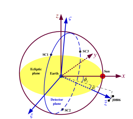
Figure 3: The schematic view of the detector plane in the GSE coordinates ($x$, $y$, $z$). $\tilde{z}$ is the normal of the detector’s plane. $\theta_{s}$ is the angle between the projection of $\tilde{z}$ on the ecliptic plane and $\tilde{z}$. $\phi_{s}$ is the angle between the direction from the earth to the sun ($x$ axis) and the projection of $\tilde{z}$ on the ecliptic plane. $\xi$ is along the intersection of the detector’s plane and the ecliptic plane, and $\zeta$ is along the intersection of a plane perpendicular to $\xi$ and the detector’s plane.

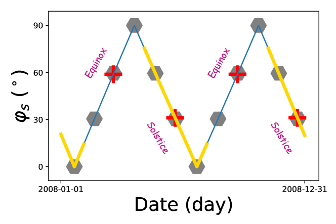
Figure 4: The time variation of $\varphi_{s}$ in the year 2008. The thick yellow lines represent the observation duration of TQ, the thin blue lines represent the non-observation duration of TQ. The red pluses mark the spring and the autumn equinoxes, the summer and the winter solstices. $\varphi_{s}$ on the grey hexagons are equal to 0^∘, 30^∘, 60^∘ and 90^∘, respectively.

The TQ detector’s plane facing the reference source is approximately perpendicular to the ecliptic plane. The global geometric structure of the bow shock and the magnetopause are quasi-axisymmetric along the Sun-Earth line ($-x$ axis in the GSE coordinates). As shown in Fig. 3, the normal of the detector’s plane is denoted as $\tilde{z}$, $\xi$ is along the intersection of the detector’s plane and the ecliptic plane, and $\zeta$ is along the intersection of a plane perpendicular to $\xi$ and the detector’s plane. Since the angle between $\tilde{z}$ and the ecliptic plane is only 4.7^∘, $\zeta$ is approximately perpendicular to the ecliptic plane. The angle $\phi_{s}$ between the direction from the sun to the earth and the projection of $\tilde{z}$ on the ecliptic plane ranges from 0 to 360^∘ annually, with $\phi_{s}=120.5^{\circ}$ at the spring equinox [19]. During one revolution of the TQ spacecraft around the Earth (3.65 days), $\phi_{s}$ can be approximately regarded as a constant. In order to describe the relative position of the TQ detector’s plane and the geometric structure of the earth magnetosphere conveniently, we transform $\phi_{s}$ to its associated acute angle $\varphi_{s}$ in the GSE coordinates. Taking the year 2008 as an example, numerical calculation based on JPL Planetary and Lunar Ephemeris DE421 [67] is adopted to evaluate the time-varying $\varphi_{s}$ which is shown as the solid lines in Fig. 4. The spring and autumn equinoxes, the summer and winter solstices are shown as red pluses. The observation windows of TQ is 2 $\times$ 3 months in one sidereal year [11]. $\varphi_{s}$ in observation windows (thick yellow lines around summer and winter solstices) and non-observation windows (thin dark blue lines around spring and autumn equinoxes) range from 0^∘ to 75.5^∘ and from 14.5^∘ to 90^∘, respectively.

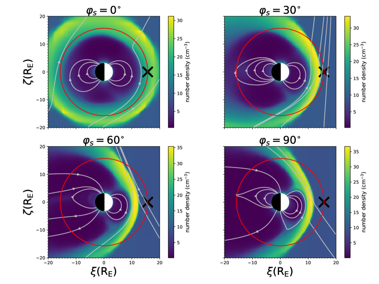
Figure 5: The electron number densities on the TQ’s detector planes where $\varphi_{s}$ = 0^∘, 30^∘, 60^∘ and 90^∘, respectively. Black crosses mark the initial phase for one of the TQ’s spacecraft. White lines are the representative magnetic field lines in the simulation domain.

In section 4, we study the acceleration noises in four representative relative positions with $\varphi_{s}$ = 0^∘, 30^∘, 60^∘, and 90^∘ which are marked as grey hexagons in Fig. 4. The hexagons on the yellow lines are in the observation window of TQ. The electron number densities for these four cases are given in Fig. 5, in which the simulation result for 2008-05-01 20:00 UT is used. The red circle represents the orbit of the spacecraft. The black crosses located at ($\xi=15.7$, $\zeta=0$) ${\rm R_{E}}$ mark the initial phase for one of the spacecraft. Two distinct boundaries around 10–20 ${\rm R_{E}}$ can be seen: the outer one is the bow shock, the inner one is the magnetopause. For $\varphi_{s}=0^{\circ}$, the bow shock and magnetopause are approximately axisymmetric, the bow shock is slightly larger than 20 ${\rm R_{E}}$, while the magnetopause is slightly larger than 10 ${\rm R_{E}}$. For $\varphi_{s}=30^{\circ}$, $60^{\circ}$ and 90^∘, the spacecraft will pass through the solar wind, the bow shock, the magnetosheath, the magnetopause, the lobes of magnetosphere and the magnetotail. We can see that as $\varphi_{s}$ decreasing the orbit will gradually shrink into the magnetosheath.

4 Results

4.1 Space plasma and magnetic field

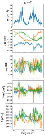
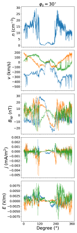
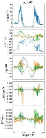
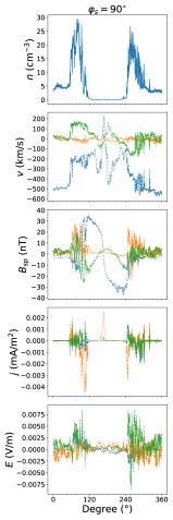
Figure 6: Distributions of ion number density $n_{i}$, bulk flow $\bm{v}$, space magnetic field $\bm{B}_{\rm sp}$, electric current $\bm{J}$ and electric field $\bm{E}_{\rm sp}$ on the orbit are in rows 1 to 5, respectively. The blue, orange and green lines in rows 2 to 5 represent the $x$, $y$, $z$ components of $\bm{v}$, $\bm{B}_{\rm sp}$, $\bm{J}$, and $\bm{E}_{\rm sp}$ in the GSE coordinates. Columns 1 to 4 denote the distributions of these parameters on the detector’s plane where $\varphi_{s}$ = 0^∘, 30^∘, 60^∘ and 90^∘. Note that the abscissa represents the orbital phase for one spacecraft in a 3.65-day circular orbit around the Earth.

On the spacecraft orbit, the values of the space plasma and magnetic field parameters are obtained from the interpolation of the ones on the 3D grid of the simulation domain. Here, the position of each spacecraft is sampled every 60 s which is in line with the time resolution of the simulation. For $\varphi_{s}=0^{\circ},30^{\circ},60^{\circ}$ and $90^{\circ}$, the number density of ion $n_{i}$, bulk flow $\bm{v}$, magnetic field $\bm{B}_{\rm sp}$, electric current $\bm{J}$ and electric field ${\bm{E}}_{\rm sp}$ on a spacecraft’s orbit are shown in Fig. 6. The dotted blue, orange and green lines represent the $x$, $y$ and $z$ components of $\bm{v}$, $\bm{B}_{\rm sp}$, $\bm{J}$ and ${\bm{E}}_{\rm sp}$, respectively. Note that ${\bm{E}}_{\rm sp}$ is calculated from $-\bm{v}\times\bm{B}_{\rm sp}$ as mentioned in section 2.3.

Take $\varphi_{s}=90^{\circ}$ as an example, combining Fig. 5 and Fig. 6, we can see that $n_{i}$ in the solar wind is lower than that in the magnetosheath, but larger than that in the magnetosphere. Meanwhile, the absolute value of $v_{x}$ is obviously larger than that of $v_{y}$ and $v_{z}$, the absolute value of $\bm{B}_{\rm sp}$ is smaller than those in the magnetosheath and magnetosphere. In the magnetosheath, the absolute values of $n_{i}$ and $\bm{B}_{\rm sp}$ are larger than those in solar wind, because that the magnetosheath is the downstream of the bow shock, $n_{i}$ and $\bm{B}_{\rm sp}$ can be enhanced by the shock [68, 46]; and the fluctuations of all these parameters are larger than those in the solar wind and the magnetosphere. In the magnetosphere, $n_{i}$ is lower than these in the solar wind and the magnetosheath, the absolute values of $\bm{B}_{\rm sp}$ is larger than that in the solar wind. In the magnetotail, the $x$ component of $\bm{B}_{\rm sp}$ reverses and the absolute value of $\bm{J}$ becomes larger, since there is a cross-tail current sheet in the magnetotail [69]. All these features are consistent with the observations [57, 70]. As $\varphi_{s}$ decreases, the TQ spacecraft will spend more time in the magetosheath and the time series of these parameters become more fluctuated.

4.2 Residual accelerations

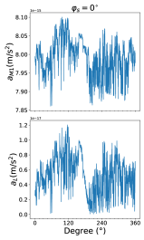
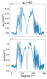
Figure 7: Distributions of $\bm{a}_{\rm M1}$ and $\bm{a}_{\rm L}$ at $\varphi_{s}$ = 0^∘, 30^∘, 60^∘ and 90^∘.

According to Equation (10)–(11) and the magnitudes of $\bm{B}_{\rm sp}$ and $\bm{E}_{\rm sp}$ on the orbit, the amplitudes of $\bm{a}_{\rm M1}$, $\bm{a}_{\rm M2}$, $\bm{a}_{\rm M3}$, $\bm{a}_{\rm M4}$ and $\bm{a}_{\rm L}$ are of the order of $10^{-14}$, $10^{-20}$, $10^{-29}$, $10^{-22}$ and $10^{-17}$ $\mathrm{m/s^{2}}$, respectively. $\bm{a}_{\rm M1}$ is the dominant acceleration noise caused by the space plasma. The time series of the acceleration noises of $\bm{a}_{\rm M1}$ and $\bm{a}_{\rm L}$ are shown in Fig. 7. Since $\bm{M}_{\rm r}\approx 20~{}\mathrm{nA~{}m^{2}}$, $\bm{M}_{\rm isc}\approx 16~{}\mathrm{nA~{}m^{2}}$, $\bm{M}_{\rm isp}\approx 0.2~{}\mathrm{nA~{}m^{2}}$, $\bm{M}_{\rm r}+2\bm{M}_{\rm isp}$ and $\bm{M}_{\rm r}+2\bm{M}_{\rm isc}$ are of the same order of magnitude, the six orders of magnitude difference between $\bm{a}_{\rm M1}$ and $\bm{a}_{\rm M2}$ is mainly due to the difference between the values of $\nabla\bm{B}_{\rm sc}$ and $\nabla\bm{B}_{\rm sp}$.

In addition, the time fluctuations of $\bm{B}_{\rm sc}$, $\nabla\bm{B}_{\rm sc}$ and $\bm{E}_{\rm sc}$ (denoted as $\delta\bm{B}_{\rm sc}$, $\delta\nabla\bm{B}_{\rm sc}$ and $\delta\bm{E}_{\rm sc}$) will result in the residual accelerations in $\bm{a}_{\rm M5}$ ($\delta\bm{E}_{\rm sc}$), $\bm{a}_{\rm M6}$ ($\delta\nabla\bm{B}_{\rm sc}$) and an additional term in $\bm{a}_{\rm M1}$ ($\delta\nabla\bm{B}_{\rm sc}$, hereafter denoted as $\bm{a}^{\prime}_{\rm M1}$). The typical value of $\delta\nabla\bm{B}_{\rm sc}$ is 10 $\rm nT/m/Hz^{1/2}$ at 0.1 mHz with the frequency dependence of $1/f^{3/2}$ [36]; and $\delta\bm{E}_{\rm sc}$ is 100 $\rm\mu V/Hz^{1/2}$ at 1 mHz [54]. The magnitude of $\bm{a}^{\prime}_{\rm M1}$, $\bm{a}_{\rm M5}$ and $\bm{a}_{\rm M6}$ can be therefore estimated as $10^{-19}$, $10^{-32}$, and $10^{-18}$ $\rm m/s^{2}/Hz^{1/2}$ at 1 mHz, respectively, which will be ignored in the following analysis.

For the MHD simulation, the ratio between displacement current density and electric current density can be approximated as follow [71, 72]:

$$\frac{\varepsilon_{0}\partial\bm{E}_{\rm sp}/\partial t}{\bm{j}}\sim\frac{E/T}{c^{2}B/L}\sim\frac{v\times BL/T}{c^{2}B}\sim\frac{v^{2}}{c^{2}},$$ (15)

where $T$, $L$ and $v$ are the typical time, length, and velocity of MHD bulk flow in the magnetosphere and the solar wind, respectively. Here $v\sim 10^{2}$ km/s in the magnetosphere or the solar wind at 1 AU. From Equation (15), we can see that the displacement current density is much lower than the electric current density. On the contrary, for the electromagnetic (EM) waves in plasma, which are ubiquitous in heliophysics [73, 74, 75], the displacement current density and the electric current density are approximately on the same order of magnitude. However, these EM waves can not be revealed in the MHD simulation. The impact of EM waves in plasma, especially on $\bm{a}_{\rm M3}$, will be subjected to our future investigations.

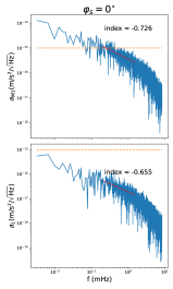
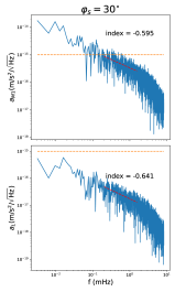
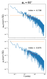
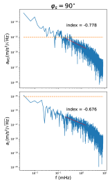
Figure 8: Amplitude spectral densities of $\bm{a}_{\rm M1}$ and $\bm{a}_{\rm L}$ at $\varphi_{s}$ = 0^∘, 30^∘, 60^∘ and 90^∘. The orange dashed horizontal lines mark the preliminary goal of the acceleration noise for TQ. The red dashed line mark the best fits of the ASDs of $\bm{a}_{\rm M1}$ and $\bm{a}_{\rm L}$.

Fig. 8 shows the amplitude spectral densities (ASDs) of the time series for $\bm{a}_{\rm M1}$ and $\bm{a}_{\rm L}$. The dashed horizontal lines ($\sqrt{S_{a}}=10^{-15}$ m/s²/Hz^1/2) mark the preliminary goal of the acceleration noise from the low-noise inertial sensor of TQ [11]. The largest contribution to the ASD of the acceleration noise is that of $\bm{a}_{\rm M1}$, while the ASD of $\bm{a}_{\rm L}$ approaches $10^{-15}$ m/s²/Hz^1/2 at the lowest frequency (1/3.65 day).

The Savitzky-Golay filter [76] is used here to smooth the ASDs of $\bm{a}_{\rm M1}$ and $\bm{a}_{\rm L}$ before the single power law fit. The fitting results are shown as the red dashed lines in Fig. 8. We can see that the lower frequency parts of the best fit spectra for $\bm{a}_{\rm M1}$ approach $10^{-15}$ m/s²/Hz^1/2 when $f\approx$ 0.24, 0.16, 0.18 and 0.17 mHz for $\varphi_{s}$ = 0^∘, 30^∘, 60^∘ and 90^∘, respectively. The corresponding spectral indexes for $\bm{a}_{\rm M1}$ ($\bm{a}_{\rm L}$) are -0.726 (-0.655), -0.595 (-0.641), -0.738 (-0.675) and -0.778 (-0.676).

Since the ASD of the acceleration noise caused by the space magnetic field ($\sqrt{S_{as}}$) is dominated by $\bm{a}_{\rm M1}$, we set $\sqrt{S_{as}}=10^{-15}$ m/s²/Hz^1/2 at 0.24 mHz and simply approximate the spectral index as $-2/3$. The ratios $\sqrt{S_{as}/S_{a}}$ are 0.38 and 0.08 at 1 mHz and 10 mHz, respectively, for the nominal values of the magnetic susceptibility ($\chi_{\rm m}=10^{-5}$) and the magnetic shielding factor ($\xi_{\rm m}=10$) of the test mass.

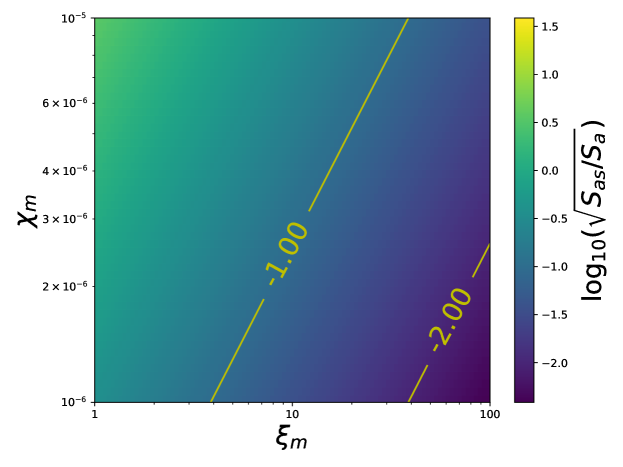
Figure 9: $\sqrt{S_{as}/S_{a}}$ at 1 mHz in the parameter space of $\xi_{\rm m}-\chi_{\rm m}$. The contours of $\sqrt{S_{as}/S_{a}}=10^{-1}$ and $10^{-2}$ are shown as yellow lines.

Note that $\xi_{\rm m}$ and $\chi_{\rm m}$ are tuneable. For LISA, the proposed value of $\xi_{\rm m}$ is of the order of 10-20 [77], a factor of 10 larger than that of LISA Pathfinder [35]. It can be further increased to 40 in the double magnetic shielding scheme [78]; the value of $\chi_{\rm m}$ is proposed to be $10^{-6}$ [35], $3\times 10^{-6}$ [36] and $4\times 10^{-6}$ [79]. Therefore, the aforementioned residual accelerations from space plasma can be regarded as an upper bound. It will be further reduced by increasing $\xi_{\rm m}$ and/or decreasing $\chi_{\rm m}$. For example, shielding TMs with multiple shields and/or with novel materials can possibly increase $\xi_{\rm m}$ several times [78]. On the other hand, the ultra-low $\chi_{\rm m}$ material for fabricating the TMs can be achieved by alloying diamagnetic and paramagnetic materials with a certain proportion [35]. Besides, $\chi_{\rm m}$ is expected to be further minimized by optimizing the fabrication process such as increasing the alloying homogeneity and avoiding the introduction of impurities. As a reference, Fig. 9 gives $\sqrt{S_{as}/S_{a}}$ at 1 mHz in the parameter space of $\xi_{m}-\chi_{m}$. The yellow lines mark the contours of $\sqrt{S_{as}/S_{a}}=10^{-1}$ and $10^{-2}$. We can see that $\sqrt{S_{as}/S_{a}}$ can be readily suppressed below $10^{-1}$ by a mild adjust from the nominal values.

5 Discussion and conclusions

In this work, we study the acceleration noises caused by the magnetic field of space plasma for the test mass of TQ, which include the contributions from the magnetic force and Lorentz force. The SWMF is adopted to simulate the global structure of the earth magnetosphere. The solar wind conditions from the ACE observations with time resolution of 60 s are taken as inputs. The MHD simulation outputs the space plasma and magnetic field parameters which are then used to calculate the acceleration noises of the test mass on the orbit of TQ’s spacecraft at $\varphi_{s}=0^{\circ},30^{\circ},60^{\circ}$ and $90^{\circ}$. It turns out that the acceleration noise produced by the interaction between the TM’s magnetic moment induced by the space magnetic field and the spacecraft magnetic field ($\bm{a}_{\rm M1}$) is the largest component with the ASD $\sqrt{S_{as}}\approx 10^{-15}$ m/s²/Hz^1/2 at $f\approx 0.2$ mHz for the nominal values of $\xi_{\rm m}$ and $\chi_{\rm m}$. $\sqrt{S_{as}/S_{a}}$ are 0.38 and 0.08 at 1 mHz and 10 mHz, respectively. We further discuss the reduction of $\sqrt{S_{as}}$ in the parameter space of $\xi_{\rm m}-\chi_{\rm m}$ which can be considered as a reference of future instrumentation development for TQ. Note that the results obtained in Sec. 4.2 depend on the values of the magnetic shielding factor and the magnetic susceptibility of the TM, for which we set $\xi_{\rm m}=10$ and $\chi_{\rm m}=10^{-5}$, respectively, as fiducial values in this work. However, in reality, $\xi_{\rm m}$ and $\chi_{\rm m}$ will be subjected to the limits from engineering consideration (build, test and launch of the spacecraft) and metallurgy. Thus, it is crucial to verify the feasibility and robustness of $\xi_{\rm m}$ and $\chi_{\rm m}$ in the future development of TQ.

The temporal resolution of our simulation is 60 s (corresponding to a Nyquist frequency of 1/120 Hz), therefore the phenomena with dynamic frequencies higher than about $10^{-2}$ Hz will not be visible. It is certainly important and will be subjected to our future investigations to study the space magnetic field with the aid from high-temporal high-spacial resolution observations and simulations.

On the other hand, the results presented here are based on the simulation from the SWMF which is a MHD model. Thus, neither the phenomena in the plasma scale, such as plasma waves and turbulences [80, 81, 82, 73], nor the associated residual accelerations can be revealed in the current work. Furthermore, in the solar wind inputs, $P_{\rm dyn}$ owns moderate values with the mean of $\approx 2.1$ (see the bottom panel of Fig. 2). However, this value can be increased significantly in the eruption events, such as ICMEs, IP shocks, magnetic reconnections, etc. The impacts of these on the TM’s residual acceleration and the spacecraft per se will be followed up.

References

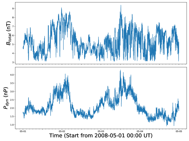
Figure 2: The input total space magnetic field ($\bm{B}_{\rm total}$) that is observed by the ACE. The solar wind dynamic pressure $P_{\rm dyn}$ is derived from the observation of the ACE.

References

- [1] B. P. Abbott, R. Abbott, T. D. Abbott, M. R. Abernathy, F. Acernese, K. Ackley, C. Adams, T. Adams, P. Addesso, R. X. Adhikari, and et al. Observation of Gravitational Waves from a Binary Black Hole Merger. Physical Review Letters, 116(6):061102, February 2016.
- [2] B. P. Abbott, R. Abbott, T. D. Abbott, M. R. Abernathy, F. Acernese, K. Ackley, C. Adams, T. Adams, P. Addesso, R. X. Adhikari, and et al. GW151226: Observation of Gravitational Waves from a 22-Solar-Mass Binary Black Hole Coalescence. Physical Review Letters, 116(24):241103, June 2016.
- [3] B. P. Abbott, R. Abbott, T. D. Abbott, F. Acernese, K. Ackley, C. Adams, T. Adams, P. Addesso, R. X. Adhikari, V. B. Adya, and et al. GW170814: A Three-Detector Observation of Gravitational Waves from a Binary Black Hole Coalescence. Physical Review Letters, 119(14):141101, October 2017.
- [4] B. P. Abbott, R. Abbott, T. D. Abbott, F. Acernese, K. Ackley, C. Adams, T. Adams, P. Addesso, R. X. Adhikari, V. B. Adya, and et al. GW170104: Observation of a 50-Solar-Mass Binary Black Hole Coalescence at Redshift 0.2. Physical Review Letters, 118(22):221101, June 2017.
- [5] B. P. Abbott, R. Abbott, T. D. Abbott, F. Acernese, K. Ackley, C. Adams, T. Adams, P. Addesso, R. X. Adhikari, V. B. Adya, and et al. GW170608: Observation of a 19 Solar-mass Binary Black Hole Coalescence. ApJ, 851:L35, December 2017.
- [6] B. P. Abbott, R. Abbott, T. D. Abbott, F. Acernese, K. Ackley, C. Adams, T. Adams, P. Addesso, R. X. Adhikari, V. B. Adya, and et al. GW170817: Observation of Gravitational Waves from a Binary Neutron Star Inspiral. Physical Review Letters, 119(16):161101, October 2017.
- [7] B. P. Abbott, R. Abbott, T. D. Abbott, S. Abraham, F. Acernese, K. Ackley, C. Adams, R. X. Adhikari, V. B. Adya, C. Affeldt, M. Agathos, K. Agatsuma, N. Aggarwal, O. D. Aguiar, L. Aiello, A. Ain, P. Ajith, G. Allen, A. Allocca, M. A. Aloy, P. A. Altin, A. Amato, A. Ananyeva, S. B. Anderson, W. G. Anderson, S. V. Angelova, S. Antier, S. Appert, K. Arai, M. C. Araya, J. S. Areeda, M. Arène, N. Arnaud, K. G. Arun, S. Ascenzi, G. Ashton, S. M. Aston, P. Astone, F. Aubin, P. Aufmuth, K. AultONeal, C. Austin, V. Avendano, A. Avila-Alvarez, S. Babak, P. Bacon, F. Badaracco, M. K. M. Bader, A. B. Zimmerman, Y. Zlochower, M. E. Zucker, J. Zweizig, LIGO Scientific Collaboration, and Virgo Collaboration. GWTC-1: A Gravitational-Wave Transient Catalog of Compact Binary Mergers Observed by LIGO and Virgo during the First and Second Observing Runs. Physical Review X, 9(3):031040, Jul 2019.
- [8] Kentaro Somiya. Detector configuration of KAGRA–the japanese cryogenic gravitational-wave detector. Classical and Quantum Gravity, 29(12):124007, jun 2012.
- [9] B. S. Sathyaprakash and B. F. Schutz. Physics, Astrophysics and Cosmology with Gravitational Waves. Living Reviews in Relativity, 12:2, March 2009.
- [10] P. Amaro-Seoane, H. Audley, S. Babak, J. Baker, E. Barausse, P. Bender, E. Berti, P. Binetruy, M. Born, D. Bortoluzzi, J. Camp, C. Caprini, V. Cardoso, M. Colpi, J. Conklin, N. Cornish, C. Cutler, K. Danzmann, R. Dolesi, L. Ferraioli, V. Ferroni, E. Fitzsimons, J. Gair, L. Gesa Bote, D. Giardini, F. Gibert, C. Grimani, H. Halloin, G. Heinzel, T. Hertog, M. Hewitson, K. Holley-Bockelmann, D. Hollington, M. Hueller, H. Inchauspe, P. Jetzer, N. Karnesis, C. Killow, A. Klein, B. Klipstein, N. Korsakova, S. L Larson, J. Livas, I. Lloro, N. Man, D. Mance, J. Martino, I. Mateos, K. McKenzie, S. T McWilliams, C. Miller, G. Mueller, G. Nardini, G. Nelemans, M. Nofrarias, A. Petiteau, P. Pivato, E. Plagnol, E. Porter, J. Reiche, D. Robertson, N. Robertson, E. Rossi, G. Russano, B. Schutz, A. Sesana, D. Shoemaker, J. Slutsky, C. F. Sopuerta, T. Sumner, N. Tamanini, I. Thorpe, M. Troebs, M. Vallisneri, A. Vecchio, D. Vetrugno, S. Vitale, M. Volonteri, G. Wanner, H. Ward, P. Wass, W. Weber, J. Ziemer, and P. Zweifel. Laser Interferometer Space Antenna. arXiv e-prints, February 2017.
- [11] J. Luo, L.-S. Chen, H.-Z. Duan, Y.-G. Gong, S. Hu, J. Ji, Q. Liu, J. Mei, V. Milyukov, M. Sazhin, C.-G. Shao, V. T. Toth, H.-B. Tu, Y. Wang, Y. Wang, H.-C. Yeh, M.-S. Zhan, Y. Zhang, V. Zharov, and Z.-B. Zhou. TianQin: a space-borne gravitational wave detector. Classical and Quantum Gravity, 33(3):035010, February 2016.
- [12] S. Kawamura, M. Ando, N. Seto, S. Sato, T. Nakamura, K. Tsubono, N. Kanda, T. Tanaka, J. Yokoyama, I. Funaki, K. Numata, K. Ioka, T. Takashima, K. Agatsuma, T. Akutsu, K.-s. Aoyanagi, K. Arai, A. Araya, H. Asada, Y. Aso, D. Chen, T. Chiba, T. Ebisuzaki, Y. Ejiri, M. Enoki, Y. Eriguchi, M.-K. Fujimoto, R. Fujita, M. Fukushima, T. Futamase, T. Harada, T. Hashimoto, K. Hayama, W. Hikida, Y. Himemoto, H. Hirabayashi, T. Hiramatsu, F.-L. Hong, H. Horisawa, M. Hosokawa, K. Ichiki, T. Ikegami, K. T. Inoue, K. Ishidoshiro, H. Ishihara, T. Ishikawa, H. Ishizaki, H. Ito, Y. Itoh, K. Izumi, I. Kawano, N. Kawashima, F. Kawazoe, N. Kishimoto, K. Kiuchi, S. Kobayashi, K. Kohri, H. Koizumi, Y. Kojima, K. Kokeyama, W. Kokuyama, K. Kotake, Y. Kozai, H. Kunimori, H. Kuninaka, K. Kuroda, S. Kuroyanagi, K.-i. Maeda, H. Matsuhara, N. Matsumoto, Y. Michimura, O. Miyakawa, U. Miyamoto, S. Miyoki, M. Y. Morimoto, T. Morisawa, S. Moriwaki, S. Mukohyama, M. Musha, S. Nagano, I. Naito, K. Nakamura, H. Nakano, K. Nakao, S. Nakasuka, Y. Nakayama, K. Nakazawa, E. Nishida, K. Nishiyama, A. Nishizawa, Y. Niwa, T. Noumi, Y. Obuchi, M. Ohashi, N. Ohishi, M. Ohkawa, K. Okada, N. Okada, K. Oohara, N. Sago, M. Saijo, R. Saito, M. Sakagami, S.-i. Sakai, S. Sakata, M. Sasaki, T. Sato, M. Shibata, H. Shinkai, A. Shoda, K. Somiya, H. Sotani, N. Sugiyama, Y. Suwa, R. Suzuki, H. Tagoshi, F. Takahashi, K. Takahashi, K. Takahashi, R. Takahashi, R. Takahashi, T. Takahashi, H. Takahashi, T. Akiteru, T. Takano, N. Tanaka, K. Taniguchi, A. Taruya, H. Tashiro, Y. Torii, M. Toyoshima, S. Tsujikawa, Y. Tsunesada, A. Ueda, K.-i. Ueda, M. Utashima, Y. Wakabayashi, K. Yagi, H. Yamakawa, K. Yamamoto, T. Yamazaki, C.-M. Yoo, S. Yoshida, T. Yoshino, and K.-X. Sun. The Japanese space gravitational wave antenna: DECIGO. Classical and Quantum Gravity, 28(9):094011, May 2011.
- [13] W. T. Ni. ASTROD Mission Concept and Measurement of the Temporal Variation in the Gravitational Constant. In Y. M. Cho, C. H. Lee, and S.-W. Kim, editors, Pacific Conference on Gravitation and Cosmology, page 309, 1998.
- [14] M. Tinto, D. Debra, S. Buchman, and S. Tilley. glisa: geosynchronous laser interferometer space antenna concepts with off-the-shelf satellites. Review of Scientific Instruments, 86(1):330, 2015.
- [15] X. Gong, Y.-K. Lau, S. Xu, P. Amaro-Seoane, S. Bai, X. Bian, Z. Cao, G. Chen, X. Chen, Y. Ding, P. Dong, W. Gao, G. Heinzel, M. Li, S. Li, F. Liu, Z. Luo, M. Shao, R. Spurzem, B. Sun, W. Tang, Y. Wang, P. Xu, P. Yu, Y. Yuan, X. Zhang, and Z. Zhou. Descope of the ALIA mission. In Journal of Physics Conference Series, volume 610 of Journal of Physics Conference Series, page 012011, May 2015.
- [16] C. Cutler and J. Harms. BBO and the Neutron-Star-Binary Subtraction Problem. Physics, 73(4):1405–1408, 2006.
- [17] G. L. Israel, W. Hummel, S. Covino, S. Campana, I. Appenzeller, W. Gässler, K.-H. Mantel, G. Marconi, C. W. Mauche, U. Munari, I. Negueruela, H. Nicklas, G. Rupprecht, R. L. Smart, O. Stahl, and L. Stella. RX J0806.3+1527: A double degenerate binary with the shortest known orbital period (321s). A&A, 386:L13–L17, May 2002.
- [18] B.-B. Ye, X. Zhang, M.-Y. Zhou, Y. Wang, H.-M. Yuan, D. Gu, Y. Ding, J. Zhang, J. Mei, and J. Luo. Optimizing orbits for TianQin. International Journal of Modern Physics D, 28:1950121, July 2019.
- [19] X.-C. Hu, X.-H. Li, Y. Wang, W.-F. Feng, M.-Y. Zhou, Y.-M. Hu, S.-C. Hu, J.-W. Mei, and C.-G. Shao. Fundamentals of the orbit and response for TianQin. Classical and Quantum Gravity, 35(9):095008, May 2018.
- [20] W.-F. Feng, H.-T. Wang, X.-C. Hu, Y.-M. Hu, and Y. Wang. Preliminary study on parameter estimation accuracy of supermassive black hole binary inspirals for TianQin. Phys. Rev. D, 99(12):123002, June 2019.
- [21] H.-T. Wang, Z. Jiang, A. Sesana, E. Barausse, S.-J. Huang, Y.-F. Wang, W.-F. Feng, Y. Wang, Y.-M. Hu, J. Mei, and J. Luo. Science with the TianQin observatory: Preliminary results on massive black hole binaries. Phys. Rev. D, 100(4):043003, August 2019.
- [22] C. Shi, J. Bao, H.-T. Wang, J.-d. Zhang, Y.-M. Hu, A. Sesana, E. Barausse, J. Mei, and J. Luo. Science with the TianQin observatory: Preliminary results on testing the no-hair theorem with ringdown signals. Phys. Rev. D, 100(4):044036, August 2019.
- [23] J. Bao, C. Shi, H. Wang, J.-d. Zhang, Y. Hu, J. Mei, and J. Luo. Constraining modified gravity with ringdown signals: An explicit example. Phys. Rev. D, 100(8):084024, October 2019.
- [24] H. Di and Y. Gong. Primordial black holes and second order gravitational waves from ultra-slow-roll inflation. J. Cosmology Astropart. Phys, 7:007, July 2018.
- [25] L.-F. Wang, Z.-W. Zhao, J.-F. Zhang, and X. Zhang. A preliminary forecast for cosmological parameter estimation with gravitational-wave standard sirens from TianQin. arXiv e-prints, July 2019.
- [26] I. H. Hutchinson. Principles of Plasma Diagnostics. 2005.
- [27] S. Y. Huang, F. Sahraoui, Z. G. Yuan, O. Le Contel, H. Breuillard, J. S. He, J. S. Zhao, H. S. Fu, M. Zhou, X. H. Deng, X. Y. Wang, J. W. Du, X. D. Yu, D. D. Wang, C. J. Pollock, R. B. Torbert, and J. L. Burch. Observations of Whistler Waves Correlated with Electron-scale Coherent Structures in the Magnetosheath Turbulent Plasma. ApJ, 861(1):29, Jul 2018.
- [28] Jichun Zhang, Michael W. Liemohn, Darren L. de Zeeuw, Joseph E. Borovsky, Aaron J. Ridley, Gabor Toth, Stanislav Sazykin, Michelle F. Thomsen, Janet U. Kozyra, Tamas I. Gombosi, and Richard A. Wolf. Understanding storm-time ring current development through data-model comparisons of a moderate storm. Journal of Geophysical Research (Space Physics), 112(A4):A04208, April 2007.
- [29] Y. Guo, M. D. Ding, Y. Liu, X. D. Sun, M. L. DeRosa, and T. Wiegelmann. Modeling Magnetic Field Structure of a Solar Active Region Corona Using Nonlinear Force-free Fields in Spherical Geometry. ApJ, 760:47, November 2012.
- [30] W. Su, Y. Guo, R. Erdélyi, Z. J. Ning, M. D. Ding, X. Cheng, and B. L. Tan. Period Increase and Amplitude Distribution of Kink Oscillation of Coronal Loop. Scientific Reports, 8:4471, March 2018.
- [31] E. N. Parker. Dynamics of the Interplanetary Gas and Magnetic Fields. ApJ, 128:664, November 1958.
- [32] R. B. Decker, S. M. Krimigis, E. C. Roelof, M. E. Hill, T. P. Armstrong, G. Gloeckler, D. C. Hamilton, and L. J. Lanzerotti. Voyager 1 in the Foreshock, Termination Shock, and Heliosheath. Science, 309(5743):2020–2024, Sep 2005.
- [33] Fran Bagenal and Peter A. Delamere. Flow of mass and energy in the magnetospheres of Jupiter and Saturn. Journal of Geophysical Research (Space Physics), 116(A5):A05209, May 2011.
- [34] M. Wang, J. Y. Lu, K. Kabin, H. Z. Yuan, X. Ma, Z. Q. Liu, Y. F. Yang, J. S. Zhao, and G. Li. The influence of IMF clock angle on the cross section of the tail bow shock. Journal of Geophysical Research (Space Physics), 121(11):11,077–11,085, Nov 2016.
- [35] Bonny L. Schumaker. Disturbance reduction requirements for LISA. Classical and Quantum Gravity, 20(10):S239–S253, May 2003.
- [36] R. T. Stebbins, P. L. Bender, J. Hanson, C. D. Hoyle, B. L. Schumaker, and S. Vitale. Current error bestimmtes for LISA spurious accelerations. Classical and Quantum Gravity, 21(5):S653–S660, Mar 2004.
- [37] J. Y. Lu, M. Wang, K. Kabin, J. S. Zhao, Z. Q. Liu, M. X. Zhao, and G. Li. Pressure balance across the magnetopause: Global MHD results. Planet. Space Sci., 106:108–115, Feb 2015.
- [38] H. Hasegawa, M. Fujimoto, T. D. Phan, H. Rème, A. Balogh, M. W. Dunlop, C. Hashimoto, and R. TanDokoro. Transport of solar wind into Earth’s magnetosphere through rolled-up Kelvin-Helmholtz vortices. Nature, 430(7001):755–758, Aug 2004.
- [39] Jiansen He, Chuanyi Tu, Eckart Marsch, and Shuo Yao. Do Oblique Alfvén/Ion-cyclotron or Fast-mode/Whistler Waves Dominate the Dissipation of Solar Wind Turbulence near the Proton Inertial Length? ApJ, 745(1):L8, Jan 2012.
- [40] F. Sahraoui, S. Y. Huang, G. Belmont, M. L. Goldstein, A. Rétino, P. Robert, and J. De Patoul. Scaling of the Electron Dissipation Range of Solar Wind Turbulence. ApJ, 777(1):15, Nov 2013.
- [41] W. Li, R. M. Thorne, V. Angelopoulos, J. Bortnik, C. M. Cully, B. Ni, O. Le Contel, A. Roux, U. Auster, and W. Magnes. Global distribution of whistler-mode chorus waves observed on the THEMIS spacecraft. Geophys. Res. Lett., 36(9):L09104, May 2009.
- [42] Steven J. Schwartz, Edmund Henley, Jeremy Mitchell, and Vladimir Krasnoselskikh. Electron Temperature Gradient Scale at Collisionless Shocks. Phys. Rev. Lett., 107(21):215002, Nov 2011.
- [43] R. C. Allen, J. C. Zhang, L. M. Kistler, H. E. Spence, R. L. Lin, B. Klecker, M. W. Dunlop, M. André, and V. K. Jordanova. A statistical study of EMIC waves observed by Cluster: 1. Wave properties. Journal of Geophysical Research (Space Physics), 120(7):5574–5592, Jul 2015.
- [44] X. Cheng, Y. Li, L. F. Wan, M. D. Ding, P. F. Chen, J. Zhang, and J. J. Liu. Observations of Turbulent Magnetic Reconnection within a Solar Current Sheet. ApJ, 866(1):64, Oct 2018.
- [45] W. Su, X. Cheng, M. D. Ding, P. F. Chen, and J. Q. Sun. A Type II Radio Burst without a Coronal Mass Ejection. ApJ, 804:88, May 2015.
- [46] W. Su, X. Cheng, M. D. Ding, P. F. Chen, Z. J. Ning, and H. S. Ji. Investigating the Conditions of the Formation of a Type II Radio Burst on 2014 January 8. ApJ, 830:70, October 2016.
- [47] S. Y. Huang, M. Zhou, F. Sahraoui, A. Vaivads, X. H. Deng, M. André, J. S. He, H. S. Fu, H. M. Li, Z. G. Yuan, and D. D. Wang. Observations of turbulence within reconnection jet in the presence of guide field. Geophys. Res. Lett., 39(11):L11104, Jun 2012.
- [48] Naoko Takahashi, Kanako Seki, Mariko Teramoto, Mei-Ching Fok, Yihua Zheng, Ayako Matsuoka, Nana Higashio, Kazuo Shiokawa, Dmitry Baishev, Akimasa Yoshikawa, and Tsutomu Nagatsuma. Global Distribution of ULF Waves During Magnetic Storms: Comparison of Arase, Ground Observations, and BATSRUS + CRCM Simulation. Geophys. Res. Lett., 45(18):9390–9397, Sep 2018.
- [49] M. Zhou, X. H. Deng, Z. H. Zhong, Y. Pang, R. X. Tang, M. El-Alaoui, R. J. Walker, C. T. Russell, G. Lapenta, R. J. Strangeway, R. B. Torbert, J. L. Burch, W. R. Paterson, B. L. Giles, Y. V. Khotyaintsev, R. E. Ergun, and P. A. Lindqvist. Observations of an Electron Diffusion Region in Symmetric Reconnection with Weak Guide Field. ApJ, 870(1):34, Jan 2019.
- [50] Gábor Tóth, Igor V. Sokolov, Tamas I. Gombosi, David R. Chesney, C. Robert Clauer, Darren L. de Zeeuw, Kenneth C. Hansen, Kevin J. Kane, Ward B. Manchester, Robert C. Oehmke, Kenneth G. Powell, Aaron J. Ridley, Ilia I. Roussev, Quentin F. Stout, Ovsei Volberg, Richard A. Wolf, Stanislav Sazykin, Anthony Chan, Bin Yu, and József Kóta. Space Weather Modeling Framework: A new tool for the space science community. Journal of Geophysical Research (Space Physics), 110(A12):A12226, Dec 2005.
- [51] P. J. Wass, H. M. Araújo, D. N. A. Shaul, and T. J. Sumner. Test-mass charging simulations for the LISA Pathfinder mission. Classical and Quantum Gravity, 22(10):S311–S317, May 2005.
- [52] Timothy J. Sumner, Guido Mueller, John W. Conklin, Peter J. Wass, and Daniel Hollington. Charge induced acceleration noise in the LISA gravitational reference sensor. Classical and Quantum Gravity, 37(4):045010, February 2020.
- [53] F. S. Mozer, R. B. Torbert, U. V. Fahleson, C. G. Falthammar, A. Gonfalone, and A. Pedersen. Electric Field Measurements in the Solar Wind, Bow Shock, Magnetosheath Magnetopause, and Magnetosphere (Article published in the special issues: Advances in Magnetospheric Physics with GEOS- 1 and ISEE - 1 and 2.). Space Sci. Rev., 22(6):791–804, Dec 1978.
- [54] F. Antonucci, M. Armano, H. Audley, G. Auger, M. Benedetti, P. Binetruy, C. Boatella, J. Bogenstahl, D. Bortoluzzi, P. Bosetti, N. Brand t, M. Caleno, A. Cavalleri, M. Cesa, M. Chmeissani, G. Ciani, A. Conchillo, G. Congedo, I. Cristofolini, M. Cruise, K. Danzmann, F. De Marchi, M. Diaz-Aguilo, I. Diepholz, G. Dixon, R. Dolesi, N. Dunbar, J. Fauste, L. Ferraioli, D. Fertin, W. Fichter, E. Fitzsimons, M. Freschi, A. García Marin, C. García Marirrodriga, R. Gerndt, L. Gesa, D. Giardini, F. Gibert, C. Grimani, A. Grynagier, B. Guillaume, F. Guzmán, I. Harrison, G. Heinzel, M. Hewitson, D. Hollington, J. Hough, D. Hoyland, M. Hueller, J. Huesler, O. Jeannin, O. Jennrich, P. Jetzer, B. Johlander, C. Killow, X. Llamas, I. Lloro, A. Lobo, R. Maarschalkerweerd, S. Madden, D. Mance, I. Mateos, P. W. McNamara, J. Mendes, E. Mitchell, A. Monsky, D. Nicolini, D. Nicolodi, M. Nofrarias, F. Pedersen, M. Perreur-Lloyd, A. Perreca, E. Plagnol, P. Prat, G. D. Racca, B. Rais, J. Ramos-Castro, J. Reiche, J. A. Romera Perez, D. Robertson, H. Rozemeijer, J. Sanjuan, A. Schleicher, M. Schulte, D. Shaul, L. Stagnaro, S. Strandmoe, F. Steier, T. J. Sumner, A. Taylor, D. Texier, C. Trenkel, D. Tombolato, S. Vitale, G. Wanner, H. Ward, S. Waschke, P. Wass, W. J. Weber, and P. Zweifel. From laboratory experiments to LISA Pathfinder: achieving LISA geodesic motion. Classical and Quantum Gravity, 28(9):094002, May 2011.
- [55] Gábor Tóth, Bart van der Holst, Igor V. Sokolov, Darren L. De Zeeuw, Tamas I. Gombosi, Fang Fang, Ward B. Manchester, Xing Meng, Dalal Najib, Kenneth G. Powell, Quentin F. Stout, Alex Glocer, Ying-Juan Ma, and Merav Opher. Adaptive numerical algorithms in space weather modeling. Journal of Computational Physics, 231(3):870–903, Feb 2012.
- [56] D. T. Welling and A. J. Ridley. Validation of SWMF magnetic field and plasma. Space Weather, 8(3):03002, Mar 2010.
- [57] A. P. Dimmock and K. Nykyri. The statistical mapping of magnetosheath plasma properties based on THEMIS measurements in the magnetosheath interplanetary medium reference frame. Journal of Geophysical Research (Space Physics), 118(8):4963–4976, Aug 2013.
- [58] Mike Liemohn, Natalia Ganushkina, Darren Zeeuw, Lutz Rastaetter, Maria Kuznetsova, Daniel Welling, Gabor Toth, Raluca Ilie, Tamas Gombosi, and Bart Holst. Real-time SWMF at CCMC: assessing the Dst output from continuous operational simulations. Space Weather, 16, 09 2018.
- [59] M. Harel, R. A. Wolf, R. W. Spiro, P. H. Reiff, C. K. Chen, W. J. Burke, F. J. Rich, and M. Smiddy. Quantitative simulation of a magnetospheric substorm 2. Comparison with observations. J. Geophys. Res., 86(A4):2242–2260, Apr 1981.
- [60] Frank Toffoletto, Stanislav Sazykin, Robert Spiro, and Richard Wolf. Inner magnetospheric modeling with the Rice Convection Model. Space Sci. Rev., 107(1):175–196, Apr 2003.
- [61] M. C. Fok and T. E. Moore. Ring current modeling in a realistic magnetic field configuration. Geophys. Res. Lett., 24(14):1775–1778, Jan 1997.
- [62] Mei-Ching Fok, Richard B. Horne, Nigel P. Meredith, and Sarah A. Glauert. Radiation Belt Environment model: Application to space weather nowcasting. Journal of Geophysical Research (Space Physics), 113(A3):A03S08, Mar 2008.
- [63] A. Glocer, G. Toth, M. Fok, T. Gombosi, and M. Liemohn. Integration of the radiation belt environment model into the space weather modeling framework. Journal of Atmospheric and Solar-Terrestrial Physics, 71(16):1653–1663, Nov 2009.
- [64] E. C. Stone, A. M. Frandsen, R. A. Mewaldt, E. R. Christian, D. Margolies, J. F. Ormes, and F. Snow. The Advanced Composition Explorer. Space Sci. Rev., 86:1–22, Jul 1998.
- [65] A. A. Samsonov, Y. V. Bogdanova, G. Branduardi-Raymont, J. Safrankova, Z. Nemecek, and J.-S. Park. Long-term variations in solar wind parameters, magnetopause location, and geomagnetic activity over the last five solar cycles. Journal of Geophysical Research: Space Physics, 124(6):4049–4063, 2019.
- [66] J. H. King and N. E. Papitashvili. Solar wind spatial scales in and comparisons of hourly Wind and ACE plasma and magnetic field data. Journal of Geophysical Research (Space Physics), 110(A2):A02104, February 2005.
- [67] W. M. Folkner, J. G. Williams, and D. H. Boggs. The Planetary and Lunar Ephemeris DE 421. Interplanetary Network Progress Report, 178:1–34, August 2009.
- [68] B. T. Draine and C. F. McKee. Theory of interstellar shocks. ARA&A, 31:373–432, 1993.
- [69] A. Runov, V. Angelopoulos, X. Z. Zhou, X. J. Zhang, S. Li, F. Plaschke, and J. Bonnell. A THEMIS multicase study of dipolarization fronts in the magnetotail plasma sheet. Journal of Geophysical Research (Space Physics), 116(A5):A05216, May 2011.
- [70] M. Wang, J. Y. Lu, K. Kabin, H. Z. Yuan, Z. Q. Liu, J. S. Zhao, and G. Li. The Influence of IMF By on the Bow Shock: Observation Result. Journal of Geophysical Research (Space Physics), 123(3):1915–1926, Mar 2018.
- [71] Francis F. Chen. Introduction to Plasma Physics and Controlled Fusion. Springer, 2016.
- [72] D. Gary Swanson. Plasma Waves (2nd edition). IOP Publishing Ltd., 2003.
- [73] S. Y. Huang, H. S. Fu, Z. G. Yuan, A. Vaivads, Y. V. Khotyaintsev, A. Retino, M. Zhou, D. B. Graham, K. Fujimoto, F. Sahraoui, X. H. Deng, B. Ni, Y. Pang, S. Fu, D. D. Wang, and X. Zhou. Two types of whistler waves in the hall reconnection region. Journal of Geophysical Research (Space Physics), 121(7):6639–6646, Jul 2016.
- [74] J. S. Zhao, Y. Voitenko, Y. Guo, J. T. Su, and D. J. Wu. Nonlinear Damping of Alfvén Waves in the Solar Corona Below 1.5 Solar Radii. ApJ, 811(2):88, October 2015.
- [75] Jinsong Zhao. Properties of Whistler Waves in Warm Electron Plasmas. ApJ, 850(1):13, Nov 2017.
- [76] A. Savitzky and M. J. E. Golay. Smoothing and differentiation of data by simplified least squares procedures. Analytical Chemistry, 36:1627–1639, January 1964.
- [77] B. Schumaker. Overview of Disturbance Reduction Requirements for LISA. Presented at 4th Int. LISA Symp. (Pennsylvania, July 2002), 2002.
- [78] A Cavalleri, G Ciani, R Dolesi, A Heptonstall, M Hueller, D Nicolodi, S Rowan, D Tombolato, S Vitale, P J Wass, and W J Weber. A new torsion pendulum for testing the limits of free-fall for LISA test masses. Classical and Quantum Gravity, 26(9):094017, apr 2009.
- [79] John Hanson, G. MacKeiser, Saps Buchman, Robert Byer, Dave Lauben, Daniel DeBra, Scott Williams, Dale Gill, Ben Shelef, and Gad Shelef. ST-7 gravitational reference sensor: analysis of magnetic noise sources. Classical and Quantum Gravity, 20(10):S109–S116, May 2003.
- [80] G. G. Howes, S. D. Bale, K. G. Klein, C. H. K. Chen, C. S. Salem, and J. M. TenBarge. The Slow-mode Nature of Compressible Wave Power in Solar Wind Turbulence. ApJ, 753(1):L19, Jul 2012.
- [81] C. S. Salem, G. G. Howes, D. Sundkvist, S. D. Bale, C. C. Chaston, C. H. K. Chen, and F. S. Mozer. Identification of Kinetic Alfvén Wave Turbulence in the Solar Wind. ApJ, 745(1):L9, Jan 2012.
- [82] S. Y. Huang, M. Zhou, F. Sahraoui, X. H. Deng, Y. Pang, Z. G. Yuan, Q. Wei, J. F. Wang, and X. M. Zhou. Wave properties in the magnetic reconnection diffusion region with high : Application of the k-filtering method to Cluster multispacecraft data. Journal of Geophysical Research (Space Physics), 115(A12):A12211, Dec 2010.
- [83] A. S. Sharma, R. Nakamura, A. Runov, E. E. Grigorenko, H. Hasegawa, M. Hoshino, P. Louarn, C. J. Owen, A. Petrukovich, J. A. Sauvaud, V. S. Semenov, V. A. Sergeev, J. A. Slavin, B. U. Ã-. Sonnerup, L. M. Zelenyi, G. Fruit, S. Haaland, H. Malova, and K. Snekvik. Transient and localized processes in the magnetotail: a review. Annales Geophysicae, 26(4):955–1006, May 2008.