Depth Selection for Deep ReLU Nets in Feature Extraction and Generalization

Abstract

Deep learning is recognized to be capable of discovering deep features for representation learning and pattern recognition without requiring elegant feature engineering techniques by taking advantage of human ingenuity and prior knowledge. Thus it has triggered enormous research activities in machine learning and pattern recognition. One of the most important challenge of deep learning is to figure out relations between a feature and the depth of deep neural networks (deep nets for short) to reflect the necessity of depth. Our purpose is to quantify this feature-depth correspondence in feature extraction and generalization. We present the adaptivity of features to depths and vice-verse via showing a depth-parameter trade-off in extracting both single feature and composite features. Based on these results, we prove that implementing the classical empirical risk minimization on deep nets can achieve the optimal generalization performance for numerous learning tasks. Our theoretical results are verified by a series of numerical experiments including toy simulations and a real application of earthquake seismic intensity prediction.

I Introduction

Asystemic machine learning process frequently comes down to two steps: feature extraction and target-driven learning. The former focuses on designing preprocessing pipelines and data transformations that result in a tractable representation of data, while the latter utilizes learning algorithms related to specific targets, such as regression, classification and clustering on the data representation to finish the learning task. Studies in the second step abound in machine learning [5] and numerous learning schemes such as kernel methods [15], neural networks [20] and boosting [21] have been proposed. However, feature extraction in the first step is usually labor intensive, which requires elegant feature engineering techniques by taking advantages of human ingenuity and prior knowledge.

To extend the applicability of machine learning, it is crucial to make learning algorithms be less dependent of human factors. Deep learning [23, 16], which has been successfully used in image classification, natural language processing and game theory, provides a promising technique in machine learning. The heart of deep learning is to adopt deep neural networks (deep nets for short) with certain structures to extract data features and design target-driven algorithms, simultaneously. As shown in Figure 1, deep learning embodies the utilities of feature extraction algorithms such as bag of feature (BOF), local binary pattern (LBP), histogram of oriented gradient (HOG) and classification algorithms like support vector machine (SVM), random forest, via tuning parameters in a unified deep nets model.

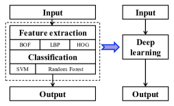
Figure 1: Magic behind deep learning

The great success of deep learning in applications demonstrates the feasibility of deep nets in specific learning tasks. However, whether deep learning is generalizable to other learning tasks relies on rigorous theoretical verifications, which is unfortunately at its infancy. In particular, it is highly desired to clarify the following three important problems: 1) which data features can be extracted by deep nets; 2) how to set the depth of deep nets in special learning tasks; 3) How about the generalization ability of deep learning algorithms. The first problem refers to the representation performance of deep nets, needing tools from information theory like coding theory [39] and entropy theory [18]. The second one concerns approximation abilities of deep nets with different depth, requiring approximation theory techniques such as local polynomial approximations [50], covering number estimates [26] and wavelets analysis [55] to quantify powers and limitations of deep nets. The last one focuses on the generalization capability of deep learning algorithms in machine learning, for which statistical learning theory as well as empirical processing [10] should be utilized.

Although lagging heavily behind applications, recent developments of deep learning theory provided some exciting theoretical results on these problems. For example, [45] proved that deep nets succeed in extracting some geometric structures of data, which has been adopted in [8] to design deep learning algorithm for regression problems with data generated on manifolds; [7] found that deep nets can extract local position information of data, which was recently employed in [31] to construct deep nets in handling sparsely located data; [39] proved that deep nets can extract piecewise features of data, which was utilized in [24] to develop learning algorithms to learn non-smooth functions efficiently. All these interesting studies presented theoretical verifications on the power of deep learning in the sense that deep nets succeed in extracting data features and deep learning significantly improves the generalization capabilities of learning schemes in-hand.

The problem is, however, there are strongly exclusive correspondences between data features and network depth for these theoretical studies in the sense that each data feature requires a unique network depth and vice-verse. To be detailed, a hierarchal structure corresponds to a hierarchal deep net with the same depth [37]; smoothness a-priori information [50] is related to a deep net with accuracy-dependent depth; a translation-invariance property requires a convolutional neural network with accuracy-dependent layers [6]; and a rotation-invariance property is associated with a deep net with tree structures and four layers [9]. Such exclusive correspondences hinder heavily the use of deep nets in feature extraction, since data features such as the smoothness information, hierarchal structure, transformation-invariance are practically difficult to be specified before the learning process. Furthermore, it is questionable to determine the network depth for simultaneously extracting multiple data features like the translation-invariance and rotation-invariance, which is pretty common in practice. Our first purpose is to break through the feature-depth correspondences by means of proving that deep nets with certain depth can extract several data features and vice-verse.

We consider extracting both single data features such as smoothness, rotation-invariance, sparseness and composite data features combining smoothness, rotation-invariance and sparseness to demonstrate the adaptivity of network depth to features and vice-verse. Intuitively, it is difficult for deep ReLU nets to extract smoothness features due to the non-smooth property of the ReLU function $\sigma(t)=\max\{t,0\}$. A natural remedy for this, as shown in [50], is to deepen the network with an accuracy-dependent depth to eliminate the negative effect of non-smoothness. Since under some specified capacity measurements such as the number of linear regions [38], Betti numbers [4], number of monomials [12] and covering numbers [18], the capacity of deep nets increases exponentially with respect to the depth, large depth usually means large capacity costs for feature extraction. Furthermore, from an optimization viewpoint, large depth requires to solve a highly nonconvex optimization problem [16, Sec. 8.2] involving the ill-conditioning of the Hessian, the existence of many local minima, saddle points, plateau and even some flat regions, making it difficult to design optimization algorithms for such deep nets with convergence guarantees. Based on these, we provide a theoretical guidance for depth selection to extract data features by showing that deep nets with various depths, larger than a specified value, are capable of extracting the smoothness and other data features. This shows an adaptivity of the depth to data features in the sense that any data features from a rich family can be extracted by deep nets with various depths. Conversely, we also provide theoretical guarantees on the adaptivity of the data feature to depths by showing that deep ReLU nets with some specific depth succeed in extracting the smoothness, spareness and composite features. All these remove the feature-depth correspondences in feature extraction for deep ReLU nets.

From feature extraction to machine learning, the tug of war between bias and variance [10] indicates that the prominent performance of deep nets in feature extraction is insufficient to demonstrate its success. The good generalization ability is frequently built upon the balance between the accuracy of feature extraction and capacity costs to achieve such an accuracy. This exhibits a bias-variance dilemma in selecting the capacity of deep nets. Different from shallow learning such as kernel methods and boosting, recent studies [22, 18] presented a depth-parameter dilemma in controlling the capacity of deep nets in the sense that different depth-parameter pairs may yield the same capacity. These two dilemmas as well as the optimization difficulty [16, Sec. 8.2] pose an urgent issue for deep learning theory on selecting the depth to guarantee the good generalization ability of deep learning algorithms. Our second purpose is not only to pursue the optimal generalization error for learning schemes based on deep nets, but also to demonstrate the depth selection strategy to realize this optimality.

We study the generalization ability of deep nets with different depths via empirical risk minimization (ERM). Based on the established adaptivity of the depth to data features in feature extraction, we establish almost optimal generalization error bounds for deep nets with numerous depth-parameter pairs. Our results show that the feature extraction step is necessary when the learning task is somewhat sophisticated and deep nets succeed in extracting deep data features of the data distribution, which illustrates the necessity of depth in deep learning. However, we also prove that the depth for realizing the optimal learning performance of deep nets is not unique. In fact, with depth larger than some specified value, all deep nets theoretically perform similarly and can achieve the optimal generalization error bounds. The only difference is that deeper nets involve less free parameters.

In a nutshell, our analysis implies three interesting findings in understanding the success of deep learning. The first is the flexibility on automatically selecting the accuracy in extracting data features via tuning the network parameters, which is different from the classical two-step learning scheme presented in Figure 1 that usually involves extremely high capacity costs to fully extract data features. The second is the versatility of deep nets with fixed depth in the sense that they can extract various data features. The third one is that if the depth is larger than a specified value, we can always get a deep net estimator with almost optimal theoretical guarantee. The problem is, however, the difficulty in solving ERM on deep nets increases with respect to the depth [16, Sec. 8.2] and [1]. Thus, it is numerically difficult and time-consuming to get a deep net estimator with large depth and there is practically an optimal depth to realize the established optimal generalization error bounds, just as our experimental results exhibit.

The rest of the paper is organized as follows. In the next section, we will introduce deep nets and show some recent developments of deep nets in feature extraction. Section 3 focuses on the depth selection for deep ReLU nets in extracting single data features, while Section 4 devotes to the depth selection in extracting composite data features. In Section 5, we are interested in the generalization error analysis for implementing ERM on deep nets. Section 6 exhibits some numerical results to verify our theoretical assertions. In the last section, we draw a simple conclusion and present some further discussions.

II Necessity of Depth in Feature Extraction

Let $d\in\mathbb{N}$ be the dimension of input space. Denote $x=(x^{(1)},\dots,x^{(d)})\in\mathbb{I}^{d}:=[-1,1]^{d}$. Let $L\in\mathbb{N}$ and $d_{0},d_{1},\dots,d_{L}\in\mathbb{N}$ with $d_{0}=d$. For $\vec{h}=(h^{(1)},\dots,h^{(d_{k})})^{T}\in\mathbb{R}^{d_{k}}$, define $\vec{\sigma}(\vec{h})=(\sigma(h^{(1)}),\dots,\sigma(h^{(d_{k})}))^{T}$. Deep ReLU nets with depth $L$ and width $d_{j}$ in the $j$-th hidden layer can be mathematically represented as

$$h_{\{d_{0},\dots,d_{L},\sigma\}}(x)=\vec{a}\cdot\vec{h}_{L}(x),$$ (1)

where

$$\vec{h}_{k}(x)=\vec{\sigma}(W_{k}\cdot\vec{h}_{k-1}(x)+\vec{b}_{k}),\qquad k=1,2,\dots,L,$$ (2)

$\vec{h}_{0}(x)=x,$ $\vec{a}\in\mathbb{R}^{d_{L}}$, $\vec{b}_{k}\in\mathbb{R}^{d_{k}},$ and $W_{k}=(W_{k}^{i,j})_{i=1,j=1}^{d_{k},d_{k-1}}$ is a $d_{k}\times d_{k-1}$ matrix. Denote by $\mathcal{H}_{\{d_{0},\dots,d_{L},\sigma\}}$ the set of all these deep nets. When $L=1$, the function defined by (1) is the classical shallow net.

The structure of deep nets is reflected by structures of weight matrices $W_{k}$ and threshold vectors $\vec{b_{k}}$ and $\vec{a}$, $k=1,2,\dots,L$. Besides the deep fully connected networks [50] that counts the number of free parameters in the $k$-th layer to be $d_{k}d_{k-1}+d_{k}$, we say that there are $n_{k}$ free parameters in the $k$-th layer, if the weight matrix $W_{k}$ and thresholds $\vec{b_{k}}$ are generated through the following three ways. The first way is that there are totally $n_{k}$ tunable entries in $W_{k}$ and $\vec{b_{k}}$, while the remainder $d_{k}d_{k-1}+d_{k}-n_{k}$ entries are fixed. An example is deep sparsely connected neural networks. The second way is that $W_{k}$ and $\vec{b_{k}}$ are exactly generated by $n_{k}$ free parameters including weight-sharing. The third way is that the weight matrix is generated jointly by both the above ways. Like the most widely used deep convolutional neural networks, we count the number of free parameters according to the third way by considering both sparse connections and weight-sharing [54, 55, 56]. It should be mentioned that such a way to count free parameter is different from [50] which considers deep fully connected neural networks. The different way to count free parameters is consistent with the structure of deep nets, which is the main reason why we can improve the approximation result of [50].

II-A Capacity measurements of deep nets

It is meaningless to pursue the outperformance of deep nets over shallow nets without considering the capacity costs, since the universality of shallow nets [11, 27] demonstrates that shallow nets can extract an arbitrary data feature as long as the network is sufficiently wide. We adopt the concept of covering number [52] which is widely used in statistical learning and information theory to measure the capacity to cast the comparison into a unified framework.

Let $\mathbb{B}$ be a Banach space and $V$ be a subset of $\mathbb{B}$. Denote by $\mathcal{N}(\varepsilon,V,\mathbb{B})$ the $\varepsilon$-covering number of $V$ under the metric of $\mathbb{B}$, which is the minimal number of elements in an $\varepsilon$-net of $V$. Intuitively, the $\varepsilon$-covering number measures the capacity of $V$ via counting the minimal number of balls in $\mathbb{B}$ with radius $\varepsilon$ covering $V$. Figure 2 showes that the $0.1$-covering number of $A$ is 19 while that of $B$ is 10, coinciding with the intuitive observation that $A$ is larger than $B$.

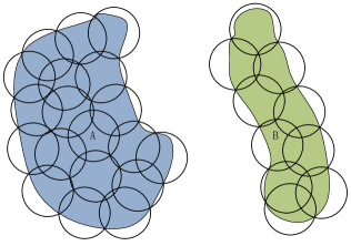
Figure 2: Covering numbers of different sets

The quantity $H(\varepsilon,V,\mathbb{B})=\log_{2}\mathcal{N}(\varepsilon,V,\mathbb{B})$ is called the $\varepsilon$-entropy of $V$ in $\mathbb{B}$ which is close to the coding length in information theory according to the encode-decode theory [13]. Thus, it is a powerful capacity measurement to show the expressivity of $V$ in $\mathbb{B}$. Furthermore, the $\varepsilon$-covering number determines the limitation of approximation ability of $V$ [18] and also the stability of learning algorithms defined on $V$ [10]. All these demonstrate the rationality of adopting the covering number to measure the capacity of deep nets.

Denote by $\mathcal{H}_{n,L}$ the set of all deep nets with $L$ hidden layers, $n$ free parameters and by

$$\mathcal{H}_{n,L,\mathcal{R}}:=\{h_{n,L}\in\mathcal{H}_{n,L}:|w_{k}^{i,j}|,|b_{k}^{i}|,|a_{i}|\leq\mathcal{R},$$

$$1\leq i\leq d_{k},1\leq j\leq d_{k-1},1\leq k\leq L\}$$ (3)

the set of deep nets whose weights and thresholds are uniformly bounded by $\mathcal{R}$, where $\mathcal{R}$ is some positive number that may depend on $n$, $d_{k}$, and $L$. The boundedness assumption is necessary since it can be found in [35, 18] that there exists some deep nets with two hidden layers and finitely many neurons possessing an infinite covering number.

The following lemma proved in [18] presents a tight estimate for the covering number of deep ReLU nets.

Lemma 1.

Let $\mathcal{H}_{n,L,\mathcal{R}}$ be defined by (II-A). Then

$$\mathcal{N}\left(\varepsilon,\mathcal{H}_{n,L,\mathcal{R}},L^{\infty}(\mathbb{I}^{d})\right)\leq\left(C\mathcal{R}D_{\max}\right)^{3(L+1)^{2}n}\varepsilon^{-n},$$ (4)

where $D_{\max}:=\max_{0\leq\ell\leq L}d_{\ell}$ and $C$ is a constant depending only on $d$.

It was deduced in [19, Chap. 16] that

$$\log\mathcal{N}(\varepsilon,\mathcal{H}_{n,1,\mathcal{R}},L^{1}(\mathbb{I}^{d}))=\mathcal{O}\left(n\log\frac{\mathcal{R}}{\varepsilon}\right).$$ (5)

Comparing Lemma 1 with (5), we find that, up to a logarithmic factor, deep nets with controllable magnitudes of weights do not essentially enlarge the capacity of shallow nets, provided that they have the same number of free parameters and the depth of deep nets is at most $\log n$. Furthermore, Lemma 1 implies that the depth plays a similar role as the number of parameters in controlling the capacity of deep nets, when $\varepsilon$ is not extremely small. This shows a novel depth-parameter dilemma in controlling the capacity and is totally different from shallow nets.

II-B Limitations of shallow nets in extracting features

The study of approximation capability of shallow nets is a classical topic in neural networks. We refer the readers to a fruitful review paper [41] for details on this topic. Compared with the classical linear approaches like polynomials, shallow nets with sigmoidal activation function possess better approximation ability [36] and are capable of conducting dimension-independent error estimates under certain restrictions on the target functions [2]. More importantly, the universality [11, 27] showed that shallow nets can extract any data feature as long as the network is sufficiently wide. However, with fixed width, they have limitations in feature extraction, in terms of saturation [33], non-localization [7, 42], non-sparse approximation [28, 31] and bottleneck in extracting the smoothness feature [35, 30]. In particular, it was shown in [35] that shallow nets whose capacity satisfies (5) cannot extract the smoothness features within accuracy $\mathcal{O}(n^{-r/(d-1)})$ with high probability, where $r$ denotes the degree of smoothness.

For shallow nets with ReLU (shallow ReLU nets), the limitation is even stricter. It was shown in [14] that there exist some analytic univariate functions which cannot be expressible for shallow ReLU nets. Recently, [50, Theorem 6] proved that any twice-differentiable nonlinear function defined on $\mathbb{I}^{d}$ cannot be $\varepsilon$-approximated by ReLU networks of fixed depth $L$ with the number of free parameters less than $c\varepsilon^{-1/(2(L-2))}$, where $c$ is a positive constant depending only on $d$. A direct consequence is that a ReLU network with depth $L=3$ and $n$ free parameters cannot extract the simple “square-feature”, i.e., $t^{2}$, within accuracy $n^{-2-\tau}$ for an arbitrary $\tau>0$. By noting $t^{2}$ is an infinitely differentiable function, it is well known that there exist linear tools to approximate $t^{2}$ within accuracy of order $n^{-\Gamma}$ [40] for an arbitrarily large $\Gamma<\infty$. All these results showed that shallow nets, especially shallow ReLU nets, are difficult to extract data features and thus have bottlenecks in complex learning tasks.

II-C Necessity of the depth for ReLU nets

Advantages of deep nets over shallow nets were firstly revealed by [7] in the sense that deep nets can provide localized approximation but shallow nets fail. Since then, a great number of data features including those for sparseness, manifold structures, piecewise smoothness and rotation-invariance are proved to be unrealizable by shallow nets but can be easily extracted by deep nets. Under the capacity constraint (4) that is similar to (5) for shallow nets, the summary of advantages of deep ReLU nets in feature extraction are listed in the following Table I.

TABLE I: Deep nets in feature extraction (within accuracy $\varepsilon$, $r$-smooth function and $d_{m}$-dimensional manifold)

Ref.	Features	Parameters	Depth
[7]	Localized approximation	$2d+1$	$2$
[31]	$k$-spatially sparse	$k(2d+1)$	$2$
[45]	Smooth+Manifold	$\varepsilon^{-d_{m}/r}$	$4$
[39]	Piecewise smooth	$\varepsilon^{-d/r}$	Finite
[42]	$\ell_{1}$ radial+smooth	$\varepsilon^{-1/r}$	$\log(\varepsilon^{-1})$
[44]	$k$-sparse (frequency)	$k\log(\varepsilon^{-1})$	$\log(\varepsilon^{-1})$

To extract the “square-feature”, the following lemma has been shown in [50, Proposition 2] to verify that deep ReLU nets can overcome the bottleneck of shallow ReLU nets.

Lemma 2.

The function $f(t)=t^{2}$ on the segment $[0,1]$ can be approximated with any error $\varepsilon>0$ by a ReLU network having the depth and free parameters of order $\mathcal{O}(\log(1/\varepsilon))$.

Due to the non-smoothness of ReLU, it is difficult for a shallow ReLU net with fixed width to extract smooth features within an arbitrary accuracy $\varepsilon$. However, by deepening the network, Lemma 2 shows that deep ReLU nets succeed in finishing such a task with only $\mathcal{O}(\log(1/\varepsilon))$ free parameters. With Lemma 2 and the relation $t_{1}\cdot t_{2}=[(t_{1}+t_{2})^{2}-t_{1}^{2}-t_{2}^{2}]/2$, deep ReLU nets can be used as a “product-gate” [50, Proposition 3] to extract the “product” relation between variables. Then, deep ReLU nets with $\mathcal{O}(\log(1/\varepsilon))$ hidden layers and free parameters can approximate arbitrary polynomials defined on $\mathbb{I}^{d}$ [44]. Therefore, even for some simple data features, deep ReLU nets theoretically beat shallow ReLU nets, showing the necessity of the depth in feature extraction. However, as shown in [16, Sec. 8.2] and [1], both the convergence issue of the stochastic gradient descent algorithm and the gradient vanishing phenomenon make it difficult to practically derive a deep ReLU net estimator, which hinders the usefulness and efficiency of Lemma 2. Figure 3 presents the difficulty for deep ReLU nets in extracting a 2-dimensional “square-feature” defined as $f(t)={t_{1}^{2}}+{t_{2}^{2}}$. For each depth, the network of the best performance is chosen and shown in the figure as a representation for the depth, by searching various (tens of) combinations of different widths and step sizes. The statistics of each depth are made from 100 trials. The relation between accuracy and depth is recorded in Figure 3 (a) and that between the frequencies of valid models and depth is recorded in Figure 3 (b). As shown, the network performs less robust when it gets deeper.

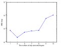
(a) Accuracy and depth

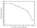
(b) Valid model and depth

Figure 3: The role of depth for approximating $t^{2}$ using SGD

III Depth Selection for Extracting a Single Feature

In this section, we introduce several data features and study the role of depth in extracting these data features to break through the feature-depth correspondences. Since there are numerous symbols involved in different data features, we provide a table of notations as follows.

TABLE II: Notations

$L$: number of layers	$n$: number of parameters
$d_{j}$: width in the $j$-th layer	$d$: input dimension
$r$: smoothness index	$\mu$ sparseness index
$\mathcal{R}$: bound of parameters	$B$: bound of polynomials
$d^{*}$: group structure dimension	$\jmath$: group structure degree

III-A Data features

In a seminal review paper [3], Bengio et al. presented a fruitful review on intuitive and experimental explanations for the success of deep learning in feature extraction. From a numerical viewpoint, deep nets can extract numerous data features including those for smoothness, hierarchical organization, shared factors, manifold structures and sparsity, part of which were theoretically verified in the recent paper [18]. In particular, [18] rigorously proved that with the similar capacity costs measured by the covering number, deep nets beat shallow nets in extracting data features listed in Table I while performing not essentially better than shallow nets in extracting the smoothness feature.

Let $f^{*}:\mathbb{I}^{d}\rightarrow\mathbb{R}$ be a function to model the potential relation between input and output, i.e., $y\approx f^{*}(x)$ with $x\in\mathbb{I}^{d}$ and $y\in\mathbb{R}$ the input variable and output variable respectively. Both structures of $x$ and properties of $f^{*}$ are regarded as data features. In the following, we introduce the smoothness feature of $f^{*}$.

Definition 1.

Let $c_{0}>0$ and $r=s+v$ with $s\in\mathbb{N}_{0}:=\{0\}\cup\mathbb{N}$ and $0<v\leq 1$. We say a function $f:\mathbb{I}^{d}\rightarrow\mathbb{R}$ is $(r,c_{0})$-smooth if $f$ is $s$-times differentiable and for every $\alpha_{j}\in\mathbb{N}_{0}$, $j=1,\dots,d$ with $\alpha_{1}+\dots+\alpha_{d}=s$, its $s$-th partial derivative satisfies the Lipschitz condition

$$\left|\frac{\partial^{s}f}{\partial x_{1}^{\alpha_{1}}\dots\partial x_{d}^{\alpha_{d}}}(x)-\frac{\partial^{s}f}{\partial x_{1}^{\alpha_{1}}\dots\partial x_{d}^{\alpha_{d}}}(x^{\prime})\right|\leq c_{0}\|x-x^{\prime}\|_{2}^{v},$$ (6)

where $x,x^{\prime}\in\mathbb{I}^{d}$ and $\|x\|_{2}$ denotes the Euclidean norm of $x$. Denote by $Lip^{(r,c_{0})}$ the set of all $(r,c_{0})$-smooth functions defined on $\mathbb{I}^{d}$.

The smoothness feature of $f^{*}$ illustrates that $x\approx x^{\prime}$ implies $f^{*}(x)\approx f^{*}(x^{\prime})$. It is a standard feature to describe $f^{*}$ and has been used in a vast literature [7, 26, 17, 39, 50, 51, 32]. However, it remains open whether deep ReLU nets can achieve the optimal performance of algebraic polynomials for realizing the smoothness feature, though encouraging developments have been made in [50, 39]. Furthermore, as pointed out in [3], the smoothness feature of $f^{*}$ is insufficient to get around the curse of dimensionality, which requires additional structure features of $x$. To this end, we introduce the following group structure feature for the input.

Definition 2.

Let $\jmath,d^{*}\in\mathbb{N}$ and $D_{1},\dots,D_{d^{*}}\in\mathbb{N}$ satisfy $d=D_{1}+\dots+D_{d^{*}}$. We say $x$ possesses a $(D_{1},\dots,D_{d^{*}})$-group structure of order $\jmath$ with respect to $f^{*}$, if there exists some polynomials $P_{k,\jmath}$, $k=1,\dots,d^{*}$ defined on $\mathbb{I}^{D_{k}}$ and of degree at most $\jmath$ and a function $g:\mathbb{R}^{d^{*}}\rightarrow\mathbb{R}$ such that

$$f^{*}(x) = g\big{[}P_{1,\jmath}(x^{(1)},\dots,x^{(D_{1})}),\dots,$$ (7)

$$P_{d^{*},\jmath}(x^{(d-D_{d^{*}}+1)},\dots,x^{(d)})\big{]}.$$

The group structure depicts the relation between different input variables. The case $d^{*}=d$ and $P_{k,\jmath}(t)=t$ for $k=1,\dots,d$ denotes that all variables in $x$ are independent. The rotation-invariance assumption [9] is included in the case $d^{*}=1$ implies that variables in $x$ possess strong dependence. The group structure assumption is more general than the manifold assumption [8], rotation-invariance assumption [9] and sparseness assumption [44] via imposing different restrictions on $P_{k,\jmath}$.

To show the outperformance of deep nets, we impose both the smoothness assumption on $f^{*}$ and group structure assumption on the input. Such a smooth-structure assumption abounds in applications. For $d^{*}=1$ and $P_{1,\jmath}(x)=(x^{(1)})^{2}+\dots+(x^{(d)})^{2}$, the smooth-structure assumption refers to a radial function that plays an important role in designing earthquake early warning systems [43]. For $d^{*}<d$ and $P_{1,\jmath}(x^{(1)},\dots,x^{(D_{1})})=(x^{(1)})^{2}+\dots+(x^{(D_{1})})^{2}$, the feature assumption is related to a partially radial function that is important in predicting the magnitude of earthquake [49]. For $d^{*}=d$ and

$${g(P_{1,\jmath}(x^{(1)}),\dots,P_{d,\jmath}(x^{(d)})=P_{1,\jmath}(x^{(1)})+\dots+P_{d,\jmath}(x^{(d)}),}$$

the smooth-structure assumption corresponds to the well known additive model [26] with polynomial kernels in statistics. If there exists some $P_{k,\jmath}(\cdot)=0$, the assumption then implies sparseness which is standard in computer vision [34].

III-B Depth selection for extracting the group structure

It was shown in [36] that for some fixed activation function, i.e., analytic and non-polynomials, shallow nets with $\left({}^{\beta+d}_{\ d}\right)$ neurons can approximate any polynomial defined on $\mathbb{I}^{d}$ of degree $\beta\in\mathbb{N}$ within an arbitrary accuracy. However, if the polynomial is sparse, then shallow nets fail to catch the sparseness information [28] in the sense that the same number of neurons is required to approximate sparse and non-sparse polynomials. However, [28, 44] found that deep nets essentially improve the performance of shallow nets by using the “product-gate” property of deep nets [50]. In particular, for deep ReLU nets, the following lemma was proved in [44, Proposition 3.3].

Lemma 3.

For any $0<\varepsilon<1$ and $\ell\in\mathbb{N}$, there exists a ReLU net $\tilde{\prod}$ with $\ell$ input units, $\mathcal{O}[(1+\log\ell)\log(\ell/\varepsilon)]$ depth and $\mathcal{O}[(1+\log\ell)\log(\ell/\varepsilon)]$ free parameters such that for any $u_{1},\dots,u_{\ell}$ satisfying $|u_{k}|\leq 1,k=1,\dots,\ell$, there holds

$$\left|\tilde{\prod}(u_{1},\dots,u_{\ell})-\prod_{k=1}^{\ell}u_{k}\right|\leq\varepsilon.$$

Noting that each monomial defined on $\mathbb{I}^{d}$ of degree at most $\beta$ can be rewritten as $\beta$ products of elements in $[0,1]$, it requires a deep net with $\mathcal{O}[(1+\log\beta)\log(\beta/\varepsilon)]$ depth and free parameters to extract the monomial feature according to Lemma 3. Based on the “product-gate-units” (PGU), we can construct a deep net such that for any $\mu$-sparse polynomials, there are only $\mu+\mathcal{O}[(1+\log\beta)\log(\beta/\varepsilon)]$ free parameters involved to extract this structure feature, which is much smaller than $\left({}^{\beta+d}_{\ d}\right)$ provided $\mu$ is small and $\varepsilon$ is not extremely small.

Although the above interesting result illustrates the power of depth in extracting structure features, the depth of the constructed deep ReLU net depends on the approximation accuracy, making it be practically difficult to get a deep net estimator, just as Figure 3 purports to show. In this paper, we pursue a trade-off between depth and number of free parameters in extracting structure features by using an approach developed in a recent paper [39]. The following “product gate” for deep ReLU nets is our main tool, whose proof can be found in Appendix A.

Lemma 4.

Let $\theta>0$ and $\tilde{L}\in\mathbb{N}$ with $\tilde{L}>(2\theta)^{-1}$. For any $\ell\in\{2,3,\dots,\}$ and $\varepsilon\in(0,1)$, there exists a deep ReLU net $\tilde{\times}_{\ell}$ with $2\ell\tilde{L}+8\ell$ layers and at most $c\ell^{\theta}\varepsilon^{-\theta}$ free parameters bounded by $\ell^{\gamma}\varepsilon^{-\gamma}$ such that

$$|u_{1}u_{2}\cdots u_{\ell}-\tilde{\times}_{\ell}(u_{1},\dots,u_{\ell})|\leq\varepsilon,\quad\forall u_{1},\dots,u_{\ell}\in[-1,1],$$

where $c$ and $\gamma$ are constants depending only on $\theta$ and $\tilde{L}$.

Comparing Lemma 4 with Lemma 3, as a “product-gate”, we reduce the depth of deep ReLU nets on the price of adding the number of free parameters. The positive number $\theta$ performs as a balance exponent in the sense that small $\theta$ implies large depth but few free parameters, while large $\theta$ means small depth but a great number of free parameters. For a fixed and $\varepsilon$-independent exponent $\theta$, the depth of ReLU nets in Lemma 4 is independent of the accuracy $\varepsilon$, while the number of free parameters increases from $\mathcal{O}[(1+\log\ell)\log(\ell/\varepsilon)]$ to $\ell^{\ell\theta}\varepsilon^{-\ell\theta}$. Therefore, Lemma 4 exhibits a trade-off between depth and parameters and removes the feature-depth correspondence.

Denote by $\mathcal{P}_{\beta}^{d}$ the set of algebraic polynomials defined on $\mathbb{I}^{d}$ with degree at most $\beta$. For $B\geq 1$, define further $\mathcal{P}_{\beta,B}^{d}:=\left\{\sum_{|\alpha|\leq\beta}c_{\alpha}x^{\alpha}:|c_{\alpha}|\leq B\right\}$ the set of polynomials in $\mathcal{P}_{\beta}^{d}$ whose coefficients are uniformly bounded by $B$, where $\alpha=(\alpha_{1},\dots,\alpha_{d})\in\mathbb{N}_{0}^{d}$, $|\alpha|=\alpha_{1}+\dots+\alpha_{d}$ and $x^{\alpha}=(x^{(1)})^{\alpha_{1}}\cdots(x^{(d)})^{\alpha_{d}}$. Define $\mathcal{P}_{\beta,B,\mu}^{d}$ the set of all $\mu$-sparse polynomials in $\mathcal{P}_{\beta,B}^{d}$. So $P\in\mathcal{P}_{\beta,B,\mu}^{d}$ has at most $\mu$ nonzero coefficients. The following theorem shows the performance of deep ReLU nets in extracting the sparse polynomial feature, whose proof will be given in Appendix A.

Theorem 1.

Let $\beta,\mu\in\mathbb{N}$, $B,\theta>0$ and $\tilde{L}\in\mathbb{N}$ with $\tilde{L}>(2\theta)^{-1}$. For any $0<\varepsilon<1$, there is a deep ReLU net structure with $2\beta\tilde{L}+8\beta+1$ layers and at most $\mu+c(\mu\beta B)^{\theta}\varepsilon^{-\theta}$ nonzero parameters bounded by $\max\{B,(\mu\beta B)^{\gamma}\varepsilon^{-\gamma}\}$, such that for each $P\in\mathcal{P}^{d}_{\beta,B,\mu}$ there exists a $h_{P}$ with the aforementioned structure satisfying

$$|P(x)-h_{P}(x)|\leq\varepsilon,\qquad\forall x\in\mathbb{I}^{d},$$

where $c$ and $\gamma$ are the constants in Lemma 4.

A similar result has been established in [44] for deep ReLU nets with depth $\mathcal{O}(\log\beta\log(\mu B\beta/\varepsilon))$ and number of free parameters $\mu+\mathcal{O}(\log\beta\log(\mu B\beta/\varepsilon))$. Our result is different from [44] by introducing an exponent $\theta$ to balance the depth and number of free parameters. For a fixed $\theta$, the depth of deep ReLU nets studied in Theorem 1 is independent of $\varepsilon$. Thus, Theorem 1 shows a novel relation between the depth and feature extraction for sparse polynomial features as well as the group structure features, by means of breaking through the exclusive feature-depth correspondence in [44]. Furthermore, if $\mu$ is not extremely small, we can select a $\theta$ in Theorem 1 such that the capacity of deep nets in Theorem 1 is smaller than that in [44] according to Lemma 1. That is, Theorem 1 provides a theoretical guidance on using smaller capacity costs than [44] to get a same accuracy in extracting the sparse feature.

III-C Deep nets for extracting the smoothness feature

In [50], Yarotsky succeeded in establishing a tight error estimate of approximating smooth functions by deep ReLU nets by utilizing the “product-gate” property in Lemma 3. [50, Theorem 1] showed that for any $f\in Lip^{(r,c_{0})}$ with $r\in\mathbb{N}$, there is a deep ReLU net $h^{\diamond}_{f}$ with fixed structure, $n$ free parameters and $\mathcal{O}(\log n)$ layers such that

$$\|f-h^{\diamond}_{f}\|_{L^{\infty}(\mathbb{I}^{d})}\leq c^{\prime}n^{-r/d}\log n,$$ (8)

where $c^{\prime}$ is a constant depending only on $c_{0}$, $d$, $r$ and $p\in[1,\infty)$. Comparing with standard results for linear approximants such as algebraic polynomials [40], there is an additional logarithmic term in (8). This is due to the accuracy-dependent depth in Lemma 3.

This phenomenon was firstly noticed in [39]. After deriving the “product-gate” property for deep ReLU nets with accuracy-independent depth, [39, Theorem 3.1] proved that there exists a deep ReLU net $h_{f}^{*}$ with fixed structure, $n$ free parameters layered on $(2+\lceil\log r\rceil)(11+r/d)$ hidden layers such that

$$\|f-h^{*}_{f}\|_{L^{p}(\mathbb{I}^{d})}\leq c^{*}n^{-r/d},$$ (9)

where $c^{*}$ is a constant depending only on $c_{0}$, $d$, $r$ and $p\in[1,{\infty})$. It is obvious that (9) improves (8) by removing the logarithmic term. However, the analysis in [39] relies on the localized approximation [7] of deep nets and thus, their result holds only under the $L^{p}(\mathbb{I}^{d})$ norm with $1\leq p<\infty$. Noting that for $f\in L^{\infty}(\mathbb{I}^{d})$, $\|f\|_{L^{p}(\mathbb{I}^{d})}\leq\|f\|_{L^{\infty}(\mathbb{I}^{d})}$, (9) does not match the optimal rate of uniform approximation by linear approximants. In the following theorem, we combine the approaches in [39] and [50] to get a sharp error estimate of approximating smooth functions by deep ReLU nets under the $L^{\infty}(\mathbb{I}^{d})$ metric.

Theorem 2.

Let $r=s+v$ with $s\in\mathbb{N}_{0}$ and $0<v\leq 1$, $c_{0},\theta>0$ and $\tilde{L}\in\mathbb{N}$ with $\tilde{L}>(2\theta)^{-1}$. For any $\varepsilon\in(0,1)$, there exists a deep ReLU net structure with

$$\mathcal{L}(d,r,\tilde{L}):=2(d+s)\tilde{L}+8(d+s)+3$$ (10)

layers and at most $c(d+s)^{\theta}\varepsilon^{-(r+d)\theta/r}+(8d+5)\left({}^{s+d}_{\ s}\right)\varepsilon^{-d/r}$ free parameters bounded by $\max\{\tilde{B},3\varepsilon^{-1/r},(d+s)^{\gamma}\varepsilon^{-(r+d)\gamma/r}\}$, such that for any $f\in Lip^{(r,c_{0})}$ there is a $h_{f}$ with the aforementioned structure satisfying

$$\|f-h_{f}\|_{L^{\infty}(\mathbb{I}^{d})}\leq c_{1}\varepsilon,$$ (11)

where $c_{1}$ is a constant depending only on $c_{0}$, $d$ and $r$ and

$$\tilde{B}:=\max_{k_{1}+\dots+k_{d}\leq s}\max_{x\in\mathbb{I}^{d}}\left|\frac{1}{k_{1}!\dots k_{d}!}\frac{\partial^{k_{1}+\dots k_{d}}f(x)}{\partial^{k_{1}}x^{(1)}\dots\partial^{k_{d}}x^{(d)}}\right|.$$

The proof of Theorem 2 will be presented in Appendix B. Setting $\varepsilon=n^{-r/d}$, we get from Theorem 2 that there exists a deep net $h_{f}$ with at most $\mathcal{O}(n^{\max\{1,(r+d)\theta/d\}})$ free parameters and $\mathcal{L}(d,r,\tilde{L})$ layers for $\tilde{L}>(2\theta)^{-1}$ such that

$$\|f-h_{f}\|_{L^{\infty}(\mathbb{I}^{d})}\leq c_{1}n^{-r/d}.$$ (12)

The depth plays a crucial role in extracting the smooth features in the sense that to derive a similar approximation accuracy as linear approximants, $\theta$ should be not larger than $d/(r+d)$, implying $\tilde{L}>(r+d)/(2d)$. However, when the depth $\mathcal{L}(d,r,\tilde{L})$ with $\tilde{L}$ reaching this critical value, deep nets with various depths are capable of extracting smooth features. This removes the feature-depth correspondence in extracting the smooth feature by making use of the structure of deep nets, since our constructed deep nets in the proof are sparse and share weights, which is different from the deep nets in the prominent work [50]. Recalling Lemma 1, for appropriately selected $\theta$, the capacity of deep nets in our construction is smaller than that of [50] by removing the logarithmic term caused by the accuracy-dependent layers. Inequalities like (11) have been established for shallow nets with some sigmoid-type activation functions [36, 29]. However, different from Theorem 2, the magnitudes of weights in [36] are so large that the capacity restriction (5) does not hold and the result in [29] suffers from the well known saturation phenomenon in the sense that the approximation rate cannot be improved any further when the smoothness of the target function goes beyond a specific level. It can be found in Theorem 2 that deepening the networks succeeds in overcoming these problems. Although [18, Theorem 2] declares that to extract the smoothness feature, deep nets perform not essentially better than shallow nets or linear approximant, our result in Theorem 2 yields that deep ReLU nets are at least not worse than shallow nets.

IV Depth Selection in Exacting Composite Features

The previous section demonstrated the role of depth in extracting a single data feature. However, as shown in [3], it is much more important to simultaneously extract multiple features to feed the target-driven learning. Extracting composite features by deep nets, which is the purpose of this section, brings novel challenges in designing deep nets, including the junction of deep nets with different utilities, the balance of accuracy and depth, and the depth-parameter trade-off.

To build up a network to exact composite features, an intuitive approach is to stack deep nets by the a-priori information or human experiences in a tandem manner, just as Figure 1 implies. The problem is, however, such a brutal stacking is practically inefficient, for both the unavailability of the a-priori information and lacking of the prescribed accuracy for extracting a specific feature. More importantly, the stacking scheme requires much more free parameters and depths of deep nets to extract composite features, adding additional capacity costs according to Lemma 1

In this section, we provide some theoretical guidance on selecting depth of deep nets to extract composite features by taking the depth-parameter trade-off into account. Without loss of generality, we are interested in extracting features exhibited in the following assumption.

Assumption 1.

Let $r=s+v$ with $s\in\mathbb{N}_{0}$ and $v\in(0,1]$, $D_{1},\dots,D_{d^{*}},d^{*}\in\mathbb{N}$ with $d=D_{1}+\dots+D_{d^{*}}$, and $\jmath,\mu\in\mathbb{N}$. Assume that there is a function $g$ defined on $\mathbb{I}^{d^{*}}$ satisfying $g\in Lip^{(r,c_{0})}$ such that (7) holds with $P_{k,\jmath}\in\mathcal{P}_{\jmath,1/2,\mu}^{D_{k}}$ for $k=1,\dots,d^{*}$.

There are totally three types of features in Assumption 1, the smoothness feature of $g$ as well as $f^{*}$, the group structure feature of $x$, and the sparsity feature of the structure polynomials $P_{k,\jmath}$, $k=1,\dots,d^{*}$. An intuitive observation is that the depth and number of free parameters of deep nets to simultaneously extract these three features should be larger than those to extract each single feature. However, as shown in the following theorem, it is not necessarily the case, provided the deep nets for different utilities are appropriately combined.

Theorem 3.

Let $r=s+v$ with $s\in\mathbb{N}_{0}$ and $v\in(0,1]$, $d^{*},\jmath,\mu\in\mathbb{N}$, $c_{0},\theta>0$ and $\tilde{L}\in\mathbb{N}$ with $\tilde{L}>(2\theta)^{-1}$. For any $0<\varepsilon<1/2$, there exists a deep ReLU net structure with at most

$$\mathcal{L}^{*}(d^{*},r,\tilde{L},\jmath)=\overbrace{\mathcal{L}(d^{*},r,\tilde{L})}^{\mbox{smooth+group}}+\overbrace{2\jmath\tilde{L}+8\jmath+1}^{\mbox{group}}$$ (13)

layers and at most

$$\mathcal{W}(d^{*},\varepsilon,\mu,\jmath,\theta):=\overbrace{(8d^{*}+5)\left({}^{s+d^{*}}_{\ s}\right)\varepsilon^{-d^{*}/r}}^{{\mbox{smooth+group}}}$$

$$+ \overbrace{\mu d^{*}}^{\mbox{sparse+group}}+\overbrace{c(d^{*}+s)^{\theta}\varepsilon^{-(r+d^{*})\theta/r}+c(\mu\jmath)^{\theta}\varepsilon^{-\theta/\tau_{r}}}^{\mbox{depth-parameter trade-off}}$$

free parameters bounded by

$$\max\{\tilde{B}_{g},3\varepsilon^{-1/r},(d^{*}+s)^{\gamma}\varepsilon^{-(r+d^{*})\gamma/r},(\mu\jmath)^{\gamma}\varepsilon^{-\gamma/\tau_{r}}\}$$ (15)

such that, for any $f^{*}$ satisfying Assumption 1, there is an $h_{f^{*}}$ possessing the aforementioned structure satisfying

$$\|f^{*}-h_{f^{*}}\|_{L^{\infty}(\mathbb{I}^{d})}\leq c_{2}\varepsilon$$

where $\tau_{r}=\left\{\begin{array}[]{cc}1,&r\geq 1,\\ v,&r<1,\end{array}\right.$ and $c_{2},\tilde{B}_{g}$ are constants depending only on $c_{0},r,d^{*}$ and $g$.

The proof of Theorem 3 will be given in Appendix C. Assumption 1 implies $f^{*}\in Lip^{(r,c_{0})}$, which requires $\mathcal{L}(d,r,\tilde{L})$ layers to extract the smoothness feature according to Theorem 2. However, with the help of the group structure feature, (13) exhibits a reduction of layers from $\mathcal{L}(d^{*},r,\tilde{L})$ to $\mathcal{L}(d,r,\tilde{L})$. To extract the group structure feature itself, additional $2\jmath\tilde{L}+8\jmath+1$ layers are required. This shows that the classical tandem stacking is not necessary. In particular, for some specific group structure features, taking $d^{*}=1$ and $\jmath=1$ for example, it is easy to select some $\theta>0$ such that $\mathcal{L}^{*}(d^{*},r,\tilde{L},\jmath)\leq\mathcal{L}(d,r,\tilde{L}),$ implying a waste of source of the tandem stacking.

The number of free parameters, as exhibited in (3), reflects the price to pay for extracting three composite features. To yield an accuracy of order $\varepsilon$, the group structure and smoothness feature require at least $\varepsilon^{-d^{*}/r}$ free parameters. It should be mentioned that this number cannot be reduced further according to [18, Theorem 2] by noting in Assumption 1 that $f^{*}$ corresponds a smooth function defined on $\mathbb{I}^{d^{*}}$. The second term in (3) reflects the difficulty in extracting the group structure feature. Without the sparseness assumption, it requires at least $\mathcal{O}\left(\sum_{k=1}^{d^{*}}\jmath^{D_{k}}\right)$ free parameters. If there is some $k$ such that $\jmath^{D_{k}}>\varepsilon^{-d^{*}/r}$, extracting the group structure feature becomes the main difficulty in the learning process. This imposes a strict restriction on $\jmath$ to maintain the optimality. The sparsity assumption reduces this risk, allowing $\jmath$ to be very large. The rest two term in (3) illustrates a depth-parameter trade-off in extracting composite features. In particular, to guarantee the optimal capability of feature extraction, $\theta$ must be smaller than the critical value $\theta_{0}:=\min\left\{\frac{d^{*}}{d^{*}+r},\frac{d^{*}\tau_{r}}{r}\right\}$. This implies a smallest depth in (13) by noting $\tilde{L}>1/(2\theta)$. In a word, less parameters requires smaller $\theta$, which results in larger $\tilde{L}$ and consequently larger $\mathcal{L}^{*}(d^{*},r,\tilde{L},\jmath)$, while more parameters require larger $\theta$, and consequently smaller $\tilde{L}$ and depth.

As Theorem 3 shows, the depth of network is not unique to extract composite features, provided it is larger than a certain level. Furthermore, our results imply two important advantages of deep nets in feature extraction. One is that, different from the classical tandem tackling, deep nets succeed in extracting composite features by embodying their interactions, and thus reduce the capacity costs. Such a reduction plays an important role in generalization, which will be analyzed in the next section. The other is the versatility of deep nets in extracting both single features and composite features in the sense that each feature corresponds to numerous depths, and vice versa. To end this section, we present two corollaries for deep nets to extract composite features. The first one is the smoothness and radial features. Let $d^{*}=1$ and $P_{1,\jmath}(x)=\frac{1}{\sqrt{d}}[(x^{(1)})^{2}+\dots+(x^{(d)})^{2}]$, then $f^{*}$ is a radial function [9]. Setting $\theta=\tau_{r}/(2+2r)$ and $\tilde{L}=2(r+1)/\tau_{r}$, we have from Theorem 3 with $\jmath=2$ and $\mu=1$ the following corollary directly.

Corollary 1.

There exists a deep ReLU net structure with $4(d+s+2)(r+1)/\tau_{r}+8(d+s)+20$ layers and at most $c_{3}n$ nonzero free parameters bounded by $c_{4}n^{\max\{1,(r+1)\gamma,\gamma r/\tau_{r}\}}$ such that for any radial function $f^{*}\in Lip^{(r,c_{0})}$ there is a deep net $h_{f^{*}}$ with the aforementioned structure satisfying

$$\|f^{*}-h_{f^{*}}\|_{L^{\infty}(\mathbb{I}^{d})}\leq c_{5}n^{-r},$$

$c_{3},c_{4},c_{5}$ are constants depending only on $c_{0},r,d$ and $f^{*}$.

The derived approximation rate is almost optimal according to [9] in the sense that the best approximation error for all deep nets satisfying the capacity restriction (4) with $n$ parameters is of order $(n/\log n)^{-r}$. Our second corollary considers using deep nets to simultaneously extract the partially radial and smooth features. Let $d^{\prime}\leq d$ and $f^{*}(x)=f(\overbrace{x^{(1)},\dots,x^{(d^{\prime})}}^{\mbox{radial}},x^{(d^{\prime}+1)},\dots,x^{(d)})=g(t_{d^{\prime}},x^{(d^{\prime}+1)},\dots,x^{(d)})$ with $t_{d^{\prime}}=(d^{\prime})^{-1/2}((x^{(d_{1})})^{2})+\dots+(x^{(d^{\prime})})^{2})\in[0,1]$. Let $\theta=\frac{(d-d^{\prime}+1)\tau_{r}}{2(d-d^{\prime}+1+r)}$ and $L=\frac{2(d-d^{\prime}+1+r)}{(d-d^{\prime}+1)\tau_{r}}$. The following corollary is a direct consequence of Theorem 3 with $d^{*}=d-d^{\prime}+1$, $\jmath=2$ and $\mu=1$.

Corollary 2.

There exists a deep ReLU net structure with

$$\frac{4(d-d^{\prime}+1+r)(d-d^{\prime}+3+s)}{(d-d^{\prime}+1)\tau_{r}}+8(d-d^{\prime}+1+s)+20$$

layers and at most $c_{6}n$ free parameters bounded by $c_{7}n^{\max\{1,(r+d-d^{\prime}+1)\gamma,\gamma r/\tau_{r}\}/(d-d^{\prime}+1)}$ such that for any partially radial function $f^{*}\in Lip^{(r,c_{0})}$ there is a deep net $h_{f^{*}}$ with the aforementioned structure satisfying

$$\|f^{*}-h_{f^{*}}\|_{L^{\infty}(\mathbb{I}^{d})}\leq c_{8}n^{-r/(d-d^{\prime}+1)},$$

where $c_{6},c_{7},c_{8}$ are constants depending only on $c_{0},r,d$ and $f^{*}$.

V Generalization Capability of Deep Nets

This section aims at the generalization capability of deep ReLU nets. Our analysis is carried out in the standard learning theory framework [10] for regression. In learning theory [10], a sample $D_{m}=\{(x_{i},y_{i})\}_{i=1}^{m}$ with $x_{i}\in\mathcal{X}=\mathbb{I}^{d}$ and $y_{i}\in\mathcal{Y}\subseteq[-M,M]$ for some $M>0$ is assumed to be drawn independently according to an unknown Borel probability $\rho$ on ${\mathcal{Z}}={\mathcal{X}}\times{\mathcal{Y}}$. The generalization capability of an estimator $f$ is measured by the generalization error, $\mathcal{E}(f):=\int_{\mathcal{Z}}(f(x)-y)^{2}d\rho$, which quantifies the relation between the sample size $m$ and prediction accuracy. The primary objective is to find an estimator based on $D_{m}$ of the regression function $f_{\rho}(x)=\int_{\mathcal{Y}}yd\rho(y|x)$ that minimizes the generalization error, where $\rho(y|x)$ denotes the conditional distribution at $x$ induced by $\rho$.

Let $\mathcal{H}_{n,L,\mathcal{R}}$ be defined by (II-A). We consider generalization error estimates for the following empirical risk minimization (ERM) on deep nets:

$$f_{D,n,L}:=\arg\min_{f\in\mathcal{H}_{n,L,\mathcal{R}}}\frac{1}{m}\sum_{i=1}^{m}[f(x_{i})-y_{i}]^{2}.$$ (16)

Since $|y_{i}|\leq M$, it is natural to project the final output $f_{D,n,L}$ to the interval $[-M,M]$ by the truncation operator $\pi_{M}f_{D,n,L}(x):=\mbox{sign}(f_{D,n,L}(x))\min\{|f_{D,n,L}(x)|,M\}.$

From Theorems 1-3, the accuracy of feature extraction decreases as the capacity of deep nets increases, resulting in small bias for the ERM. However, too large capacity makes ERM be sensitive to noise and leads to large variance. This is the well known bias-variance dilemma [10, Chap.1]. The optimal generalization performance for ERM is obtained by balancing the bias and variance, just as Figure 4 (a) purports to show. For ERM on deep nets, the problem is that the capacity depends on both depth and number of free parameters. As shown in Figure 4 (b), all $(L,n)$ pairs in the curve “A” share the same covering number bounds in Lemma 1 with $\varepsilon=0.01$. In summary, there are two dilemmas to get a good generalization for ERM on deep nets: bias-variance dilemma in selecting the capacity and depth-parameter dilemma in controlling the bias. The purpose of our study is not only to pursue the optimal generalization error for ERM on deep nets, but also to derive feasible candidates of $(L,n)$ pairs to realize the optimality. The main result is the following theorem.

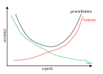
(a) Bias-variance trade-off

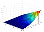
(b) Depth-width trade-off

Figure 4: Bias-variance trade-off for ERM on deep nets

Theorem 4.

Let $0<\delta<1$, $r=s+v$ with $s\in\mathbb{N}_{0}$ and $0<v\leq 1$, $\mu,\jmath,d,d^{*}\in\mathbb{N}$ and $f_{D,n,L^{*}}$ be defined by (16) with $L^{*}=\mathcal{L}^{*}(d^{*},r,\tilde{L},\jmath)$, $\mathcal{R}$ be the value given in (15), $n=\left[C_{1}m^{\frac{d^{*}}{2r+d^{*}}}\right]$ and elements in $\mathcal{H}_{L,\mathcal{R},n}$ possess the same structure as that in Theorem 3. If $f_{\rho}$ satisfies Assumption 1, $\tilde{L}>(2\theta)^{-1}$ with

$$0<\theta\leq\theta_{0}:=\min\left\{\frac{d^{*}}{d^{*}+r},\frac{d^{*}\tau_{r}}{r}\right\},$$ (17)

and

$$\mu\jmath\leq n^{\frac{\tau_{r}d^{*}+\theta}{d^{*}\tau_{r}\theta}},\qquad\mbox{and}\quad\mu\leq n,$$ (18)

then

$$\mathcal{E}(\pi_{M}f_{D,n,L^{*}})-\mathcal{E}(f_{\rho})\leq C_{2}\tilde{L}^{2}m^{-\frac{2r}{2r+d^{*}}}\log m\log\frac{3}{\delta}$$ (19)

holds with confidence of at least $1-\delta$, where $C_{1},C_{2}$ are constants independent of $\delta$, $m$, $\tilde{L}$ or $n$.

The proof of Theorem 4 will be given in Appendix D. Condition (18) presents a restriction on the group structure and sparsity features in the sense that either $\mu$ or $\jmath$ should be relatively small with respect to the size of data. It should be noted that the established learning rate cannot be essentially improved in the sense that for some special $P_{k,\jmath}$, the learning rate is optimal [9, Theorem 3]. We emphasize that the learning rate in the above theorem is much better than the optimal learning rate $m^{-\frac{2r}{2r+d}}$ for learning $(r,c_{0})$-smooth functions on $\mathbb{I}^{d}$ [19, 31]. As pointed out in [9], even restricting to learning a radial function, to achieve a learning rate similar to (19) with $d^{*}=1$, it requires at least $[m^{\frac{d-1}{2r+1}}]$ neurons to guarantee the generalization error of order $m^{-\frac{2r}{2r+1}}$. This shows the outperformance of deep nets over shallow nets.

Theorem 4 also shows the almost optimal learning rates for deep nets in learning data with the group structure and smoothness features. The relation $n=\left[C_{1}m^{\frac{d^{*}}{2r+d^{*}}}\right]$ is obtained by the bias-variance trade-off principle. It should be mentioned that there is an additional $L^{2}$ in right-hand sides of (19), implying advantages of small depth. However, (17) implies that there is a critical depth, larger than which deep nets with suitable structures can achieve the almost optimal generalization error bounds. It also exhibits a depth-parameter trade-off in the sense that small $\theta$ results in small number of parameters. A different $\theta$ thus provides different $(L,n)$ pairs to realize the optimal generalization performance of ERM on deep ReLU nets.

VI Experimental Results

In this section, we present both toy simulations and real data experiments to show the roles of depth for ReLU nets in feature selection and prediction. All the numerical experiments are carried out in the Python-3.5.4 environment running on a workstation with a Pascal Titan X 12-GB GPU and 24-GB memory. Our implementation is derived from the publicly available Tensorflow-1.4.0 framework by using AdamOptimizer. Our codes are available at http://vision.sia.cn/our%20team/Hanzhi-homepage/vision-ZhiHan%28English%29.html.

VI-A Experimental setting

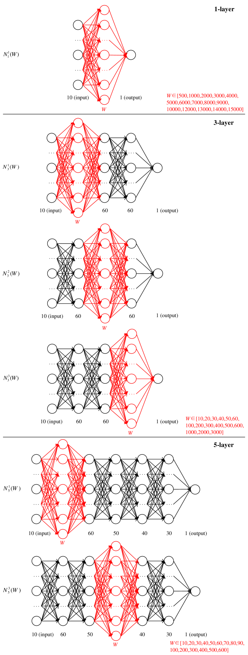
Figure 5: Network architectures of various depths and widths.

The settings of simulations are described as follows.

Implementation and Evaluation: The are five purposes in our experimental study. The first one is to verify the adaptivity of depths to the feature. The second one is to declare the adaptivity of features to the depth. The third one aims at demonstrating the necessity of depth in feature extraction. The fourth one focuses on the necessity of depths in generalization. In our last experiment, we show the power of deep nets in some real applications. In each simulation, we randomly generate $m$ sample points $\{x_{i}\}_{i=1}^{m}$ on $\mathcal{X}\in\mathbb{R}^{d}$ according to the uniform distribution. Each $x_{i}$ corresponds to an output $y_{i}$ with either $y_{i}=f(x_{i})$ (Sections 6.2, 6.3, 6.4) or $y_{i}=f(x_{i})+\varepsilon_{i}$ (Section 6.5) with $\varepsilon_{i}$ some Gaussian noise. We repeat 10 times and record the average values of the following five quantities:

$\bullet$ Mean squared error (MSE): given an estimator $f_{D}$, MSE, defined by $\frac{1}{m}\sum_{i=1}^{m}(f_{D}(x_{i})-y_{i})^{2}$, measures the average squared difference between the estimated values and what is estimated. It is a standard measurement to quantify the prediction performance of an estimator.

$\bullet$ Mean absolute error (MAE): MAE, defined by $\frac{1}{m}\sum_{i=1}^{m}|f_{D}(x_{i})-y_{i}|$, quantifies the fitting performance of $f_{D}$. It is another popular measurement, which is less sensitive to outliers than MSE, to quantify the prediction performance.

$\bullet$ Median absolute error (MdAE): MdAE, defined by $m_{0.5}(\left|f_{D}(x_{i})-m_{0.5}(y_{i})\right|)$, is a robust measure of the variability of an estimator, where $m_{0.5}$ means a median. Thus, MdAE, together with MAE, shows the robustness of the estimator.

$\bullet$ R squared score (R²S): R²S, defined by $R^{2}S(y,f)=1-\frac{{\sum_{i=1}^{n}(y_{i}-f_{D}(x_{i}))}^{2}}{{\sum_{i=1}^{n}(y_{i}-\bar{y})}^{2}}$ with $\bar{y}=\frac{1}{m}\sum_{i=1}^{m}y_{i}$, is a statistical measurement that represents the proportion of the variance of an estimate by that of real outputs in a regression model. It measures the fitness of the model.

$\bullet$ Explained variance score (EVS): EVS, defined by $1-\frac{{\sum_{i=1}^{m}(y_{i}-f_{D}(x_{i}))}^{2}}{\sum_{i=1}^{m}y_{i}^{2}},$ measures the proportion to which a mathematical model accounts for the variation (dispersion) of a given data set.

All these measurements quantify the prediction performance of an estimator in terms of the prediction accuracy, sensitivity to outliers, robustness and fitness.

Structures of deep nets: Generally speaking, there are four components in describing the structure of deep nets: depth, width in each layer, sparsity in conjunction, and sharing weights. In our experiments, network width is equivalent to the number of neurons. If the sparsity in conjunction and sharing weights are considered, there are too many structures even for a three-layer feed-forward network. Thus, we are only concerned with fully connected deep nets with different width and depth. In fact, we train over 200 networks of different depths and widths in our simulations. We use $N_{L}^{\ell}(W)$ to represent a network of $L$ layers and width $W$ in the $\ell$-th layer (marked as red as in Figure 5). For example, $N_{3}^{2}(100)$ and $N_{3}^{2}(200)$ are both 3-layer networks. The widths in layer-1 and layer-3 are fixed. The only difference is the widths in layer-2 are $100$ and $200$, respectively. In Figure 5, we present some examples for the structures adopted in our simulations. The details of structures will be explained in each simulation, if it is needed.

VI-B Adaptivity of the Depth to features

In this subsection, we study the performance of deep nets in extracting the 10-dimensional “square-feature”:

$$f(x)=\sum_{j=1}^{10}(x^{(j)})^{2},$$

where $x=(x^{(1)},\dots,x^{(10)})$ is i.i.d. generated according to the uniform distribution on $[-100,100]^{10}$. The sizes of training dataset and testing dataset are $3000$ and $200$, respectively. Our purpose is to show the adaptivity of structures to the square feature, i.e., there are various structures to extract the square feature.

VI-B1 The necessity of depth

For comparison, we train 135 networks of different depths and widths. The network architectures are illustrated in Figure 5. In particular, we choose 3 different depths $L=\{1,3,5\}$ and select 15 different widths, which are shown in different colors in Figure 6 and marked in different curves.

As shown in Figure 6, all the curves show similar patterns, i.e., along with the increasement of width, the MSE decreases at the beginning and increases later. The difference is, for the deeper networks, it generally needs smaller width to reach the best performance. The average widths in the varied layers corresponding to the best performance networks of 1-layer, 3-layer and 5-layer are 4000, 60 and 52, respectively.

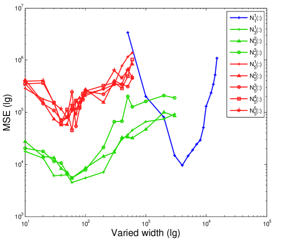
Figure 6: MSE curves of networks with various structures

The outperformance of 3-layer over shallow nets in Figure 6 verifies the necessity of depth and show that deep nets can extract the square feature better than shallow nets with much fewer neurons. The superiority of 3-layer over 5-layer deep nets demonstrates that there exists an optimal depth in extracting some specific feature. Here the optimality means not only the optimal accuracy, but also the solvability or convergence of the adopted AdamOptimizer algorithm, since its convergence issue is questionable when the depth increases [16]. Thus, although Theorem 1 proved that there are numerous depth-parameter pairs achieving the same accuracy, the convergence issue suggests to set the depth as small as possible.

VI-B2 Role of the width for 3-layer deep nets

Theorem 1 presents a relation between the depth and the number of free parameters in extracting the square feature. However, it does not give any guidance on the distribution of the width in each hidden layer. In this experiment, we fix the total number of parameters of a 3-layer network at 8000 (slightly variation is allowed, and the range is $[8000,8100]$). We manually change width of each layer, the numbers of parameters connecting Input and Layer-1 ($C_{1}$), connecting Layer-1 and Layer-2 ($C_{2}$), connecting Layer-2 and Layer-3 ($C_{3}$), and connecting Layer-3 and Output ($C_{4}$). Hence we generate a group of networks (20 in total) with different representative parameter distributions. The details of the networks are listed in Appendix E.

We record the testing errors in Figure 7, where each spot represents one network and the coordinates $(p(C_{1}),p(C_{2}),p(C_{3}))$ are the percentage of the parameters occupied. As $p(C_{1})+p(C_{2})+p(C_{3})+p(C_{4})=1$, the 3-layer networks of various distributions can be uniquely positioned by this 3-dimensional coordinate system. The size of the spot represents the MSE of the corresponding network, i.e., smaller spot indicates smaller MSE. To be noted, the biggest MSE that can be reflected by the size of the spot is 10000. The networks with MSE larger than 10000 are represented by yellow spots, while the red spots mean the corresponding networks do not converge at all.

Figure 7 exhibits two phenomena for deep nets in feature extraction. The first one is the huge impact of the width distribution. The pattern shown in this experiment is that more connections between Layer-1 and Layer-2 ($p(C_{2})$) generally bring better results, while a large number of connections with Input or Output layers ($p(C_{1})$ or $p(C_{4})$) lead to bad performances. This phenomenon indicates why a network is usually designed in a spindle shape. The other one is the adaptivity of the structure to the “square-feature”. It can be found in Figure 7 that all green points perform similarly, which means that if the depth is suitable selected, then there is a large range of the width distributions such that deep nets with such distributions succeed in extracting the “square-feature”.

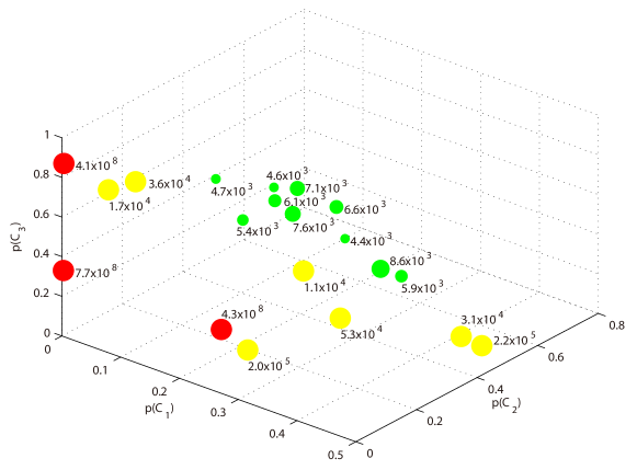
Figure 7: Networks with various width distributions.

VI-C Adaptivity of features to the depth

In Theorems 1-3, it was proved that deep nets with fixed depth can extract different data features including the sparsity, group structure, and smoothness. In this simulation, we aim to verify this adaptivity of the feature to structures. We are interested in partially radial features defined by

$$f_{k}(x)=\sum_{j=1}^{k}(x^{(j)})^{2}+\sum_{j=k+1}^{10}x^{(j)},$$

where $x$ is generated by uniformly sampling from $[-100,100]^{10}$.

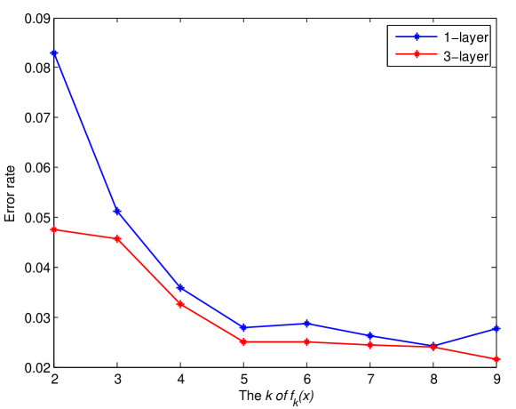
Figure 8: Adaptivity of the feature to structures.

In the experiment, besides verifying the adaptivity of deep nets, we also compare the performances between deep nets and shallow nets to show the necessity of depth in extracting different data features. As $k$ varies from $2$ to $9$, the structure of deep nets (3-layer net) is fixed as $50-60-60$, while the widths in shallow nets is selected according to the test data directly to optimize their performance.

Figure 8 shows the result curves (the detailed numerical results can be found in Appendix F). It can be seen that a deep net with fixed structures performs robustly for dealing with different data features, and always outperforms shallow nets. This demonstrates adaptivity of features to structures. Additionally, we are also aware during the experiment that training shallow nets requires more iterations.

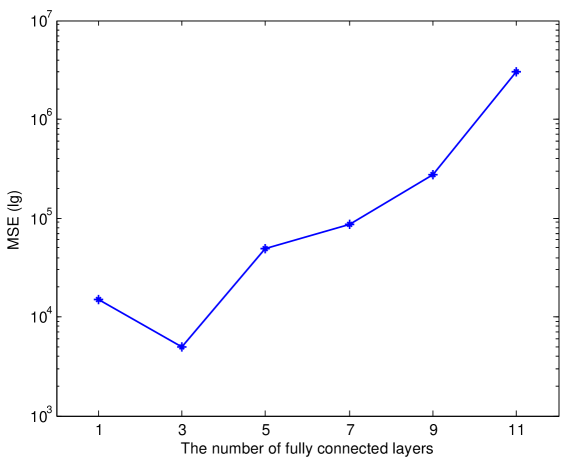
Figure 9: Best results from networks of different depths.

VI-D The role of depth in network

In this subsection, we study the role of depth in extracting the 10-dimensional “square-feature”. The simulation setting is the same as that in Subsection 6.2. The only difference is that we select more deep nets with different structures to perceive the impact of depth. There are six candidates for the depth, $1$, $3$, $5$, $7$, $9$ and $11$ and the width is chosen according to the test data directly from much more candidates than those in Subsection 6.2. In particular, the number of neurons in the widest layers of are $4000$, $60$, $30$, $30$, $9$ and $6$, respectively. The MES curve of simulation results is shown in Figure 9 (the detailed numerical results can be found in Appendix G).

It is shown that the depth plays a crucial role in improving the performance of neural networks in feature extraction. We can see that a deep net performs better than a shallow net, but a larger depth does not necessarily lead to better performance. For this simple case (single feature), deep nets with 3 layers are enough. Besides the MSE curve in Figure 9, Table IX presented MSE, MAE, MdAE, R²S and EVS results for the same purpose. All these measurements exhibit similar patterns to that of MSE in Figure 9 and verify both the necessity of depth in feature extraction and limitations of deep nets with too many hidden layers.

VI-E Generalization capability verification

In this experiment, in order to test the generalization ability of networks, we train networks with noisy data in a more complex relationship. The underlying relationship between the input signal $x=(x_{1},x_{2})$ and output is:

$$y=\sin\|x\|_{2}^{2}/\|x\|_{2}^{2}+\varepsilon,$$

where $\varepsilon\sim\mathcal{N}(0,\sigma^{2})$ is the Gaussian noise with the variance of $\sigma^{2}$. The training and test points are generated by i.i.d. sampling 2000 and 200 points on $[-1,1]$ according to the uniform distribution, respectively, and the noise level is set $\sigma^{2}=0.1$.

TABLE III: Network width candidates.

Depth	Range of width	Step length
$1$	$[16,192]$	$16$
$2$	$[4,32]$	$4$
$3$	$[4,16]$	$4$
$4$	$[4,16]$	$4$
$5$	$[4,16]$	$4$
$6$	$[4,16]$	$4$

We compare the optimal MSE of deep nets of different depths. The optimal results are obtained by tuning two important parameters, the descent step (learning rate during network training) and the width of each layer. During the training process, the descent step changes dynamically as follow,

$$R_{d}=R_{0}*D^{\lfloor(S_{g}/S_{d})\rfloor},$$

where $\lfloor\cdot\rfloor$ is the floor function, $R_{0}$ is the initial descent step and $R_{d}$ is the decayed descent step, $D$ is the decay rate, $S_{g}$ and $S_{d}$ are global step and decay step, respectively. Global step represents the current iteration number. Decay step controls the change frequency of descent step. For example, in this experiment, the decay step is $1000$, and $D$ is $0.95$. The descent step decays to $95\%$ every 1000 iterations. For choosing adequate $R_{0}$, we tried values of $0.0001$, $0.0005$ and $0.001$ on various networks of different depths. Empirically, we notice that a deeper network needs a smaller descent step. Therefore, in the experiment, the descent step is $0.001$ for $1$, and $0.0005$ for $2$, $3$, $4$, $5$ and $6$-layer networks.

The optimal widths of networks are chosen from a group of candidates, which are set empirically. Table III shows the details. For example, for a 3-layer network, the width candidates of each layer are $\{4,8,12,16\}$. As a result, there are $4^{3}$ networks for testing. To alleviate the test burden, in the experiment, we first fix widths of non-middle layers at the medians of the corresponding ranges and test the middle layer width with all the candidates to elect the optimal one, then we tune other layers one by one by testing the candidates around the optimal width of the middle layer.

In Figure 10, we recorded the optimal MSE and the rate of valid model of deep nets with different depths. Noting that the function $\sin\|x\|_{2}^{2}/\|x\|_{2}^{2}$ is smooth and radial, which are difficult for shallow nets to extract them simultaneously, according to the theoretical results in [9]. In our simulation, we show that combining the feature extraction with target-driven learning in deep net is feasible. In fact, a deep net with four layers can significantly improve the performance of shallow nets. Table IV presents the regression result in terms of MSE, MAE, MdAE, R²S, and EVS, respectively and exhibits the same pattern as that of MSE in Figure 10.

(a) Accuracy and depth

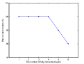
(b) Valid model and depth

Figure 10: The generalization error result of deep nets.

TABLE IV: Noisy data training by networks of various depths.

Depth	1-layer	2-layer	3-layer	4-layer	5-layer	6-layer
MAE	$0.0765$	$0.0760$	$0.0741$	$0.0731$	$0.0755$	$0.0772$
MSE	$0.0923$	$0.0712$	$0.0705$	$0.0694$	$0.0718$	$0.1265$
MdAE	$0.0755$	$0.0745$	$0.0743$	$0.0708$	$0.0731$	$0.0770$
R2S	$-1.2481$	$-1.2040$	$-0.7588$	$-0.8710$	$-1.6787$	${-3.9073\times 10^{11}}$
EVS	$0.5909$	$0.5925$	$0.5943$	$0.5957$	$0.0674$	${-2.3854\times 10^{11}}$

TABLE V: The experiment results on synthetic seismic intensity dataset.

Depth	1-layer	2-layer	3-layer	4-layer	5-layer	6-layer
MAE	$0.176$	$0.125$	$0.054$	$0.036$	$0.061$	$0.25$
MSE	$0.0578$	$0.0312$	$0.0049$	$0.0037$	$0.0074$	$0.1684$
MdAE	$0.151$	$0.091$	$0.051$	$0.049$	$0.064$	$0.16$
R2S	$0.939$	$0.97$	$0.995$	$1.0$	$0.99$	$0.859$
EVS	$0.939$	$0.97$	$0.995$	$1.0$	$0.99$	$0.859$

VI-F Applications for the earthquake seismic intensity prediction

For verifying our theoretical assertions on real applications, in this subsection, we do experiments on earthquake seismic intensity estimations. Earthquake early warning (EEW) systems serve as the tools for coseismic risk reduction. One of the challenges in the development of EEW systems is the accuracy of seismic intensity estimation at the largest possible warning time. Seismic intensity is the intensity or severity of ground shaking at a given location. The level of seismic intensity depends heavily on the distance between the observation site and the epicenter. It can be realized that the level of seismic intensity is a radial function by taking the epicenter as the origin. In the experiments, we test on synthetic data and then deal with a real world dataset.

VI-F1 Synthetic data experiment

The Modified Mercalli intensity scale (MM or MMI), descended from Giuseppe Mercalli’s Mercalli intensity scale of 1902, is the most used seismic intensity scale for measuring the intensity of shaking at a given location. It has been a common sense that seismic intensity is an expression of the amplitude, duration and frequency of ground motion. Thus, many attempts have been made to estimate MMI with the ground motion parameters [46]. Fourier amplitude spectrum (FAS) is one of the best features meeting the requirement based on which [47] gives an estimation of MMI as

$$\begin{aligned} &MMI=\exp\{1.2655+0.2089\mathcal{M}\\ &-0.0011d-0.2451\log(d+2.1502\mathcal{M})\},\end{aligned}$$ (20)

where $d$ is the estimated Joyner-Boore distance (in kilometers), and $\mathcal{M}$ is the moment magnitude. Figure 11 shows a dense synthetic MMI map generated by (20).

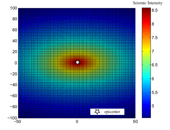
Figure 11: Dense synthetic MMI map generated by (20).

For network testing, we generate 900 samples according to (20) for training networks of 6 different depths. The testing results are reported in Figure 12 and Table V. Similar to the experiment in Subsection VI-E, networks perform well and the best result is also given by a 4-layer network.

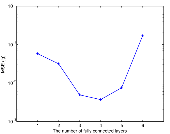
Figure 12: MSE curve of network during training on synthesis synthetic intensity dataset.

VI-F2 Real data experiment

For the real data experiment, data are from the U.S. Earthquake Intensity Database, which collects damage and felt reports for over 23,000 U.S. earthquakes. The digital database contains information regarding epicentral coordinates, magnitudes, focal depths, names and coordinates of reporting cities (or localities), reported intensities, and the distance from the city (or locality) to the epicenter. Some samples of the data are shown in Figure 13. The input of networks in this experiment are the latitude and longitude coordinates of the site where the earthquake occurred (green box), and the output is seismic intensity (red box). As the seismic intensity values in the database are integers in $\{2,\dots,6\}$ , we consider this task as a classification problem rather than a regression problem.

In order to have enough data for network training, we collect the most data impacted by the same epicenter from the dataset as the experiment data. There are total $608$ samples, in which, $500$ are used for training and the rest $108$ for testing. The parameter tuning strategy is similar to that of Section VI-E. Table VI shows the comparison results between deep nets of different depths and traditional classification methods, i.e., support vector machine (SVM) and random forest (RF). It is shown that a 5-layer deep net gives the best performance, while networks with other depths cannot compete with SVM.

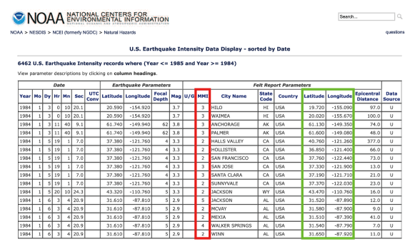
Figure 13: U.S. Earthquake Intensity Data

TABLE VI: Comparisons with traditional methods.

Method		Recognition rate
SVM		$62.96\%$
Random forest		$58.33\%$
Deep networks	1-layer	$57.41\%$
	3-layer	$60.1\%$
	5-layer	66.67%
	7-layer	$62.03\%$

VII Conclusion

In this paper, we studied theoretical advantages of deep nets via considering the role of depth in feature extraction and generalization. The main contributions are four folds. Firstly, under the same capacity costs (via covering numbers), we proved that deep nets are better than shallow nets in extracting the group structure features. Secondly, we proved that deep ReLU nets are one of the optimal tools in extracting the smoothness feature. Thirdly, we rigorously proved the adaptivity of features to depths and vice verse, which was adopted to derive the optimal learning rate for implementing empirical risk minimization on deep nets. Finally, we conducted extensive numerical experiments including toy simulations and real data verifications to show the outperformance of deep nets in feature extraction and generalization. All these results presented reasonable explanations for the success of deep learning and provided solid guidance on using deep nets. In this paper, we only consider the depth selection in regression problems. It would be interesting and important to develop similar conclusions for classification. We will consider this topic and report progress in our future study later.

Appendix A: Proofs of Theorem 1

In Appendix A, we prove Lemma 4 and Theorem 1. Our main tool is the following lemma, which can be found in [39, Lemma A.3].

Lemma 5.

Let $\theta>0$ and $\tilde{L}\in\mathbb{N}$ with $\tilde{L}>(2\theta)^{-1}$. For any $\varepsilon\in(0,1)$, there exists a deep ReLU net $\tilde{\times}_{2,\tilde{L},\varepsilon}$ with $2\tilde{L}+8$ layers and at most $c\varepsilon^{-\theta}$ nonzero parameters which are bounded by $\varepsilon^{-\gamma}$ such that

$$|uu^{\prime}-\tilde{\times}_{2,\tilde{L},\varepsilon}(u,u^{\prime})|\leq\varepsilon,\qquad\forall\ u,u^{\prime}\in[-2,2],$$

where $c,\gamma$ are positive constants depending only on $\tilde{L}$ and $\theta$.

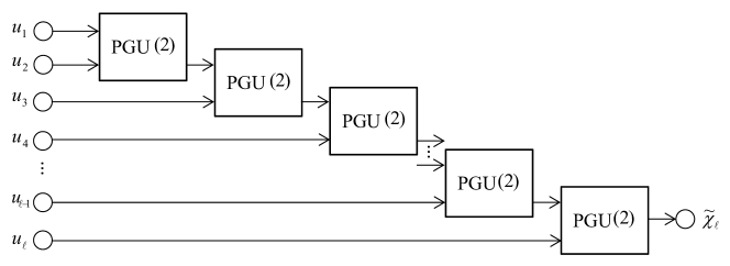
Figure 14: Network structure for PGU($\ell$)

Based on the above lemma, we can construct product gate units (PGUs) for multiple factors. In particular, there are numerous network structures for extending PGU with 2 factors to PGU with $\ell>2$ factors. We only prove that a network structure shown in Figure 14 is suitable for this purpose in Lemma 4.

Proof:

For $j=2,\dots,\ell$ and $\varepsilon\in(0,1)$, define

$$\tilde{\times}_{j,\tilde{L},\varepsilon/\ell}(u_{1},\dots,u_{j})$$

$$:= \overbrace{\tilde{\times}_{2,\tilde{L},\varepsilon/\ell}(\tilde{\times}_{2,\tilde{L},\varepsilon/\ell}(\cdots\tilde{\times}_{2,\tilde{L},\varepsilon/\ell}}^{j-1}(u_{1},u_{2}),\cdots,u_{u_{j-1}}),u_{j}).$$

Then,

$$u_{1}u_{2}\cdots u_{\ell}-\tilde{\times}_{\ell,\tilde{L},\varepsilon/\ell}(u_{1},\dots,u_{\ell})$$

$$= u_{1}u_{2}\cdots u_{\ell}-\tilde{\times}_{2,\tilde{L},\varepsilon/\ell}(u_{1},u_{2})u_{3}\cdots u_{\ell}$$

$$+ \tilde{\times}_{2,\tilde{L},\varepsilon/\ell}(u_{1},u_{2})u_{3}\cdots u_{\ell}-\tilde{\times}_{3,\tilde{L},\varepsilon/\ell}(u_{1},u_{2},u_{3})u_{4}\cdots u_{\ell}$$

$$+ \dots$$

$$+ \tilde{\times}_{\ell-1,\tilde{L},\varepsilon/\ell}(u_{1},\dots,u_{\ell-1})u_{\ell}-\tilde{\times}_{\ell,\tilde{L},\varepsilon/\ell}(u_{1},\dots,u_{\ell}).$$

But Lemma 5 implies

$$|\tilde{\times}_{2,\tilde{L},\varepsilon/\ell}(u,u^{\prime})|\leq|u||u^{\prime}|+\varepsilon/\ell\leq|u|+\varepsilon/\ell,\quad\forall\ u,u^{\prime}\in[-1,1].$$

This together with $0<\varepsilon<1$ and $u_{i}\in[-1,1]$ for all $i=1,2,\dots,\ell$ yields

$$|\tilde{\times}_{j,\tilde{L},\varepsilon/\ell}(u_{1},\dots,u_{j})|$$

$$\leq |\tilde{\times}_{j-1,\tilde{L},\varepsilon/\ell}(u_{1},\dots,u_{j-1})|+\varepsilon/\ell$$

$$\leq \dots\leq|\tilde{\times}_{2,\tilde{L},\varepsilon/\ell}(u_{1},u_{2})|+(j-2)\varepsilon/\ell$$

$$\leq 1+(j-1)\varepsilon/\ell\leq 2,\qquad\forall\ j=2,\dots,\ell.$$

Then, it follows from Lemma 5 again that

$$|u_{1}u_{2}\cdots u_{\ell}-\tilde{\times}_{\ell,\tilde{L},\varepsilon/\ell}(u_{1},\dots,u_{\ell})|$$

$$\leq |u_{1}u_{2}-\tilde{\times}_{2,\tilde{L},\varepsilon/\ell}(u_{1},u_{2})|$$

$$+ |\tilde{\times}_{2,\tilde{L},\varepsilon/\ell}(u_{1},u_{2})u_{3}-\tilde{\times}_{3,\tilde{L},\varepsilon/\ell}(u_{1},\dots,u_{3})|+\dots$$

$$+ |\tilde{\times}_{\ell-1,\tilde{L},\varepsilon/\ell}(u_{1},\dots,u_{\ell-1})u_{\ell}-\tilde{\times}_{\ell,\tilde{L},\varepsilon/\ell}(u_{1},\dots,u_{\ell})|$$

$$\leq (\ell-1)\varepsilon/\ell<\varepsilon.$$

Since $\tilde{\times}_{2,\tilde{L},\varepsilon/\ell}$ is a deep net with $2\tilde{L}+8$ layers and at most $c\ell^{\theta}\varepsilon^{-\theta}$ nonzero parameters bounded $\ell^{\gamma}\varepsilon^{-\gamma}$ and the parameters in all PGU(2) are the same, $\tilde{\times}_{\ell,\tilde{L},\varepsilon/\ell}$ is a deep net with at most $(2\tilde{L}+8)\ell$ layers, and at most $c\ell^{\theta}\varepsilon^{-\theta}$ non-zero parameters which are bounded by $\ell^{\gamma}\varepsilon^{-\gamma}$. Setting $\tilde{\times}_{\ell}=\tilde{\times}_{\ell,\tilde{L},\varepsilon/\ell}$, we complete the proof of Lemma 4. ∎

We are now in a position to prove Theorem 1.

Proof:

By Lemma 4, for any $\varepsilon\in(0,1),$ $\theta>0$ and $\tilde{L}$ with $\tilde{L}>(2\theta)^{-1}$ there exists a deep ReLU net $\tilde{\times}_{\beta}$ with at most $(2\tilde{L}+8)\beta$ layers, and at most $c(\mu B\beta)^{\theta}\varepsilon^{-\theta}$ non-zero parameters which are bounded by $(\mu B\beta)^{\gamma}\varepsilon^{-\gamma}$ such that

$$|u_{1}u_{2}\cdots u_{\beta}-\tilde{\times}_{\beta}(u_{1},\dots,u_{\beta})|\leq\frac{\varepsilon}{\mu B},\quad\forall u_{1},\dots,u_{\beta}\in[-1,1].$$ (21)

Then, for any monomial

$$x^{\alpha}=\overbrace{x^{(1)}\cdots x^{(1)}}^{\alpha_{1}}\cdots\overbrace{x^{(d)}\cdots x^{(d)}}^{\alpha_{d}}\cdot\overbrace{1\cdots 1}^{\beta-|\alpha|}$$

satisfying $|\alpha|\leq\beta$, it follows from (21) that

$$|x^{\alpha}-\tilde{\times}_{\beta}(\overbrace{x^{(1)},\dots,x^{(1)}}^{\alpha_{1}},\dots,\overbrace{x^{(d)},\dots,x^{(d)}}^{\alpha_{d}},\overbrace{1,\dots,1}^{\beta-|\alpha|})|\leq\frac{\varepsilon}{\mu B}.$$

Rewrite $P\in\mathcal{P}_{\beta,B,\mu}^{d}$ as $P=\sum_{\alpha\in\Lambda_{\mu}}c_{\alpha}x^{\alpha}$ with $|c_{\alpha}|\leq B$, where $\Lambda_{\mu}\subseteq\{\alpha:|\alpha|\leq\beta\}$ is a set of at most $\mu$ elements. Define

$$h_{P}(x)=\sum_{\alpha\in\Lambda_{\mu}}c_{\alpha}\tilde{\times}_{\beta}(\overbrace{x^{(1)},\dots,x^{(1)}}^{\alpha_{1}},\dots,\overbrace{x^{(d)},\dots,x^{(d)}}^{\alpha_{d}},\overbrace{1,\dots,1}^{\beta-|\alpha|}).$$ (22)

Then,

$$|h_{P}(x)-P(x)|\leq\sum_{\alpha\in\Lambda_{\mu}}|c_{\alpha}|\frac{\varepsilon}{\mu B}\leq\varepsilon.$$

Since the parameters in PGU($\beta$) are shared to be same, $\mu$ different $\alpha\in\Lambda_{L}$ activate $\mu$ PGU($\beta$), there are totally $\mu+c(\mu B\beta)^{\theta}\varepsilon^{-\theta}$ free parameters in $h_{P}$, which are distributed in $(2\tilde{L}+8)\beta+1$ and bounded by $(\mu B\beta)^{\gamma}\varepsilon^{-\gamma}$. This completes the proof of Theorem 1. ∎

Appendix B: Proof of Theorem 2

We need a construction of deep nets motivated by [50]. For $t\in\mathbb{R}$, define

$$\psi(t)=\sigma(t+2)-\sigma(t+1)-\sigma(t-1)+\sigma(t-2).$$ (23)

Then,

$$\psi(t)=\left\{\begin{array}[]{cc}1,&|t|\leq 1,\\ 0,&|t|\geq 2,\\ 2-|t|,&1<|t|<2.\end{array}\right.$$ (24)

Furthermore, for $N\in\mathbb{N}$ and $\mathbf{j}=(j_{1},\dots,j_{d})\in\{0,1,\dots,N\}^{d},$ define

$$\phi_{{\bf j},N}(x)=\prod_{k=1}^{d}\psi\left(3N\left(x^{(k)}-\frac{j_{k}}{N}\right)\right).$$ (25)

Direct computation yields

$$\sum_{{\bf j}\in\{0,1,\dots,N\}^{d}}\phi_{{\bf j},N}(x)=1,\qquad\forall\ x\in\mathbb{I}^{d}$$ (26)

and

$$\mbox{supp}\phi_{{\bf j},N}\subseteq\{x:|x^{(k)}-j_{k}/N|<1/N,\forall k\},$$ (27)

where $\mbox{supp}f$ denotes the support of the function $f$. Before presenting the proof of Theorem 2, we introduce two technical lemmas. The first one can be found in [25, Lemma 1].

Lemma 6.

Let $r=s+v$ with $s\in\mathbb{N}_{0}$ and $0<v\leq 1$. If $f\in Lip^{(r,c_{0})}$, $x_{0}\in\mathbb{R}^{d}$ and $p_{s,x_{0},f}$ is the Taylor polynomial of $f$ with degree $s$ at around $x_{0}$, then

$$|f(x)-p_{s,x_{0},f}(x)|\leq\tilde{c}_{1}\|x-x_{0}\|_{2}^{r},\qquad\forall\ x\in\mathbb{I}^{d},$$ (28)

where $\tilde{c}_{1}$ is a constant depending only on $s$, $c_{0}$ and $d$.

The second one focuses on approximating functions in $Lip^{(r,c_{0})}$ by products of Taylor polynomials and ReLU nets.

Lemma 7.

For $f\in Lip^{(r,c_{0})}$ with $r=s+v$, $N\in\mathbb{N}$ and ${\bf j}/N=(j_{1}/N,\dots,j_{d}/N)$, define

$$f_{1}(x)=\sum_{\mathbf{j}\in\{0,1,\dots,N\}^{d}}\phi_{{\mathbf{j}},N}(x)p_{s,{\bf j}/N,f}(x),$$ (29)

then

$$|f(x)-f_{1}(x)|\leq\tilde{c}_{2}N^{-r},\qquad\forall x\in\mathbb{I}^{d},$$ (30)

where $\tilde{c}_{2}$ is a constant depending only on $r$, $c_{0}$ and $d$.

Proof:

Due to (26), (27), $0\leq\phi_{\bf j,N}(x)\leq 1$ and Lemma 6, we have

$$|f(x)-f_{1}(x)|$$

$$= \left|f(x)-\sum_{\mathbf{j}\in\{0,\dots,N\}^{d}}\phi_{{\mathbf{j}},N}(x)p_{s,{\bf j}/N,f}(x)\right|$$

$$\leq \sum_{\mathbf{j}\in\{0,\dots,N\}^{d}}\phi_{{\mathbf{j}},N}(x)|f(x)-p_{s,{\bf j}/N,f}(x)|$$

$$\leq \sum_{\mathbf{j}:|x^{(k)}-j_{k}/N|<1/N,\forall k}|f(x)-p_{s,{\bf j}/N,f}(x)|$$

$$\leq 2^{d}\max_{\mathbf{j}:|x^{(k)}-\mathbf{j}_{k}/N|<1/N,\forall k}|f(x)-p_{s,{\bf j}/N,f}(x)|$$

$$\leq 2^{d}\tilde{c}_{1}\max_{\mathbf{j}:|x^{(k)}-\mathbf{j}_{k}/N|<1/N,\forall k}\|x-\mathbf{j}/N\|_{2}^{r}$$

$$\leq \tilde{c}_{1}2^{d}\sqrt{d^{r}}N^{-r}.$$

This proves Lemma 7 with $\tilde{c}_{2}=\tilde{c}_{1}2^{d}\sqrt{d^{r}}$. ∎

With these helps, we prove Theorem 2 as follows.

Proof:

Rewrite

$$f_{1}=\sum_{{\bf j}\in\{0,1,\dots,N\}^{d}}\sum_{\alpha:|\alpha|\leq s}a_{{\bf j},\alpha}\phi_{{\bf j},N}(x)x^{\alpha}$$ (31)

with $|a_{{\bf j},\alpha}|\leq\tilde{B}.$ Then for arbitrarily fixed $\alpha$ with $|\alpha|\leq s$ and ${\bf j}\in\{0,1,\dots,N\}^{d}$, we can rewrite

$$\phi_{{\bf j},N}(x)x^{\alpha}$$

$$= \overbrace{x^{(1)}\cdots x^{(1)}}^{\alpha_{1}}\cdots\overbrace{x^{(d)}\cdots x^{(d)}}^{\alpha_{d}}\cdot\overbrace{1\cdots 1}^{s-|\alpha|}\prod_{k=1}^{d}\psi_{k}(x),$$

where

$$\psi_{k}(x)=\psi\left(3N\left(x^{(k)}-\frac{j_{k}}{N}\right)\right).$$ (32)

But Lemma 4 shows that for any $0<\nu<1$ and $u_{1},\dots,u_{s+d}\in[-1,1]$, there exists a deep net $\tilde{\times}_{d+s}$ with $2(d+s)\tilde{L}+8(d+s)$ layers and at most $c(d+s)^{\theta}\nu^{-\theta}$ free parameters which are bounded by $(d+s)^{\gamma}\nu^{-\gamma}$ such that

$$|u_{1}u_{2}\cdots u_{d+s}-\tilde{\times}_{d+s}(u_{1},\dots,u_{d+s})|\leq\nu.$$ (33)

Define

$$h_{f}(x) := \sum_{{\bf j}\in\{0,1,\dots,N\}^{d}}\sum_{\alpha:|\alpha|\leq s}a_{{\bf j},\alpha}\tilde{\times}_{d+s}\big{(}\psi_{1}(x),\dots,\psi_{d}(x),$$ (34)

$$\overbrace{x^{(1)},\cdots x^{(1)}}^{\alpha_{1}},\dots,\overbrace{x^{(d)},\dots x^{(d)}}^{\alpha_{d}},\overbrace{1,\dots,1}^{s-|\alpha|}\big{)}.$$

Note that $h_{f}$ possesses $(N+1)^{d}\left({}^{s+d}_{\ s}\right)$ PGU($d+s$), $\tilde{\times}_{d+s}$, with the same parameters and also involves $(N+1)^{d}\left({}^{s+d}_{\ s}\right)$ $\Psi_{k}(\cdot)$. But (23) and (32) show that there are totally $8d+4$ free parameters for each $\Psi_{k}(\cdot),k=1,\dots,d$. Therefore, there are totally $2(s+d)\tilde{L}+8(s+d)+3$ layers and at most $c(d+s)^{\theta}\nu^{-\theta}+(8d+5)(N+1)^{d}\left({}^{s+d}_{\ s}\right)$ free parameters which are bounded by $\max\{\tilde{B},3N,(d+s)^{\gamma}\nu^{-\gamma}\}$ in $h_{f}$. Furthermore, (34), (33) and (31) yield that for arbitrary $x\in\mathbb{I}^{d}$,

$$|f_{1}(x)-h_{f}(x)| \leq \sum_{{\bf j}\in\{0,1,\dots,N\}^{d}}\sum_{\alpha:|\alpha|\leq s}|a_{{\bf j},\alpha}|\varepsilon$$

$$\leq (N+1)^{d}\left({}^{s+d}_{\ s}\right)\tilde{B}\nu.$$

Recalling Lemma 7, we have

$$|f(x)-h_{f}(x)|\leq\tilde{c}_{2}N^{-r}+(N+1)^{d}\left({}^{s+d}_{\ s}\right)\tilde{B}\nu.$$

Setting $N+1=\left[\nu^{-1/(d+r)}\right]$, we obtain

$$|f(x)-h_{f}(x)|\leq\tilde{c}_{3}\nu^{r/(r+d)},$$

where $\tilde{c}_{3}:=\tilde{c}_{2}+2^{d}\left({}^{s+d}_{\ s}\right)\tilde{B}.$ Denote $\varepsilon=\nu^{r/(r+d)}$. Then, for any $\varepsilon\in(0,1)$, $h_{f}$ is a deep net with $2(d+s)\tilde{L}+8(d+s)+3$ layers and at most $c(d+s)^{\theta}\varepsilon^{-(r+d)\theta/r}+(8d+5)\left({}^{s+d}_{\ s}\right)\varepsilon^{-d/r}$ free parameters which are bounded by $\max\{\tilde{B},3\varepsilon^{-1/r},(d+s)^{\gamma}\varepsilon^{-(r+d)\gamma/r}\}$ satisfying

$$|f(x)-h_{f}(x)|\leq\tilde{c}_{3}\varepsilon,$$

This completes the proof of Theorem 2. ∎

Appendix C: Proof of Theorem 3

Proof:

For any $0<\nu_{1}<1/2$, $\theta>0$, $\tilde{L}\in\mathbb{N}$ with $\tilde{L}>(2\theta)^{-1}$ and $k=1,\dots,d^{*}$, it follows from Theorem 1 that there is deep ReLU net $h_{P_{k,\jmath}}$ with at most $2\jmath\tilde{L}+8\jmath+1$ layers and at most $\mu+c(\mu\jmath)^{\theta}\nu_{1}^{-\theta}$ nonzero parameters which are bounded by $(\mu\jmath)^{\gamma}\nu_{1}^{-\gamma}$ such that

$$|P_{k,\jmath}(x)-h_{P_{k,\jmath}}(x)|\leq\nu_{1},\qquad\forall x\in\mathbb{I}^{D_{k}},k=1,\dots,d^{*}.$$ (35)

Since $|P_{k,\jmath}(x)|\leq 1/2$ for $x\in\mathbb{I}^{d}$, we have from (35) and $0<\nu_{1}\leq 1/2$ that $|h_{P_{k,\jmath}}(x)|\leq 1$. Define

$$h_{d^{*}}(x)=(h_{P_{1,\jmath}}(x),h_{P_{2,\jmath}}(x),\dots,h_{P_{d^{*},\jmath}}(x)).$$

Let $g$ be the $d^{*}$-dimensional function in Assumption 1, i.e.,

$$f^{*}(x)=g(P_{1,\jmath}(x),\dots,P_{d^{*},\jmath}(x)).$$

For arbitrary $0<\nu_{2}<1$, Theorem 2 shows that there is deep net $h_{g}$ with $\mathcal{L}(d^{*},r,\tilde{L})$ layers and at most $c(d^{*}+s)^{\theta}\nu_{2}^{-(r+d^{*})\theta/r}+(8d^{*}+5)\left({}^{s+d^{*}}_{\ s}\right)\nu_{2}^{-d^{*}/r}$ free parameters which are bounded by $\max\{\tilde{B}_{g},3\nu_{2}^{-1/r},(d^{*}+s)^{\gamma}\nu_{2}^{-(r+d^{*})\gamma/r}\}$ such that

$$\|g-h_{g}\|_{L^{\infty}(\mathbb{I}^{d^{*}})}\leq c_{1}\nu_{2},$$ (36)

where

$$\tilde{B}_{g}:=\max_{k_{1}+\dots+k_{d^{*}}\leq\jmath}\max_{x\in\mathbb{I}^{d}}\left|\frac{1}{k_{1}!\dots k_{d^{*}}!}\frac{\partial^{k_{1}+\dots k_{d^{*}}}f(x)}{\partial^{k_{1}}x^{(1)}\dots\partial^{k_{d}}x^{({d^{*}})}}\right|$$

Define

$$h_{f^{*}}(x)=h_{g}(h_{d^{*}}(x)).$$ (37)

For arbitrary $x\in\mathbb{I}^{d}$, there holds

$$|f^{*}(x)-h_{f^{*}}(x)|$$

$$= |g(P_{1,\jmath}(x),\dots,P_{d^{*},\jmath}(x))-h_{g}(h_{d^{*}}(x))|$$

$$\leq |g(P_{1,\jmath}(x),\dots,P_{d^{*},\jmath}(x))-g(h_{d^{*}}(x))|$$

$$+ |g(h_{d^{*}}(x))-h_{g}(h_{d^{*}}(x))|.$$

Due to the smoothness of $g$, we have from (35) and (6) that

$$|g(P_{1,\jmath}(x),\dots,P_{d^{*},\jmath}(x))-g(h_{d^{*}}(x))|$$

$$\leq \tilde{c}_{4}\max_{1\leq k\leq d^{*}}|P_{k,\jmath}(x)-h_{P_{k,\jmath}}(x)|^{\tau_{r}}\leq\tilde{c}_{4}\nu_{1}^{\tau_{r}},$$

where $\tilde{c}_{4}>0$ is a constant depending only on $c_{0}$, $d^{*}$ and $g$. But (36) yields

$$|g(h_{d^{*}}(x))-h_{g}(h_{d^{*}}(x))|\leq c_{1}\nu_{2},\qquad\forall\ x\in\mathbb{I}^{d}.$$

Thus, we have

$$|f^{*}(x)-h_{f^{*}}(x)|\leq c_{1}\nu_{2}+\tilde{c}_{4}\nu_{1}^{\tau_{r}}.$$

Set $\nu_{2}=\nu_{1}^{\tau_{r}}=\varepsilon$. Then for any $0<\varepsilon\leq 1/2$, we get

$$|f^{*}(x)-h_{f^{*}}(x)|\leq\tilde{c}_{5}\varepsilon,$$

where $\tilde{c}_{5}$ is a constant depending only on $c_{0},d,d^{*},r,s$ and $g$. Under this circumstance, $h_{f^{*}}$ is a deep net with

$$\mathcal{L}^{*}(d^{*},r,\tilde{L},\jmath)=\mathcal{L}(d^{*},r,\tilde{L})+2\jmath\tilde{L}+8\jmath+1$$

layers and at most

$$c(d^{*}+s)^{\theta}\varepsilon^{-\frac{(r+d^{*})\theta}{r}}+(8d^{*}+5)\left({}^{s+d^{*}}_{\ s}\right)\varepsilon^{-\frac{d^{*}}{r}}+d^{*}\mu+c(\mu\jmath)^{\theta}\varepsilon^{-\frac{\theta}{\tau_{r}}}$$

free parameters which are bounded by

$$\max\{\tilde{B}_{g},3\varepsilon^{-1/r},(d^{*}+s)^{\gamma}\varepsilon^{-(r+d^{*})\gamma/r},(\mu\jmath)^{\gamma}\varepsilon^{-\gamma/\tau_{r}}\}.$$

This completes the proof of Theorem 3. ∎

Appendix D: Proof of Theorem 4

In this section only, $C_{1}^{\prime},C_{2}^{\prime},\dots$ denote constants independent of $L$, $n$, $\varepsilon$, $\delta$, $\mu$ or $\jmath$. To prove Theorem 4, we need the following well-known oracle inequality in learning theory, the proof of which can be found in [9].

Lemma 8.

Let $\rho_{X}$ be the marginal distribution of $\rho$ on $\mathcal{X}$ and $(L^{2}_{\rho_{{}_{X}}},\|\cdot\|_{\rho})$ denote the Hilbert space of square-integrable functions on $\mathcal{X}$ with respect to $\rho_{X}$. Set $\mathcal{E}_{D}(f):=\frac{1}{m}\sum_{i=1}^{m}(f(x_{i})-y_{i})^{2}$ and define

$$f_{D,\mathcal{H}}=\arg\min_{f\in\mathcal{H}}\mathcal{E}_{D}(f),$$ (38)

where $\mathcal{H}$ is a set of functions defined on $\mathcal{X}$. Suppose further that there exist $n^{\prime},\mathcal{U}>0$, such that

$$\log\mathcal{N}(\varepsilon,\mathcal{H},L^{\infty}(\mathbb{I}^{d}))\leq n^{\prime}\log\frac{\mathcal{U}}{\varepsilon},\qquad\forall\varepsilon>0.$$ (39)

Then for any $h\in\mathcal{H}$,

$$Prob\{\|\pi_{M}f_{D,\mathcal{H}}-f_{\rho}\|_{\rho}^{2}>\varepsilon+2\|h-f_{\rho}\|_{\rho}^{2}\}$$

$$\leq \exp\left\{n^{\prime}\log\frac{16\mathcal{U}M}{\varepsilon}-\frac{3m\varepsilon}{512M^{2}}\right\}$$

$$+ \exp\left\{\frac{-3m\varepsilon^{2}}{16(3M+\|h\|_{L_{\infty}(\mathcal{X})})^{2}\left(6\|h-f_{\rho}\|_{\rho}^{2}+\varepsilon\right)}\right\}.$$

Now we apply Lemma 8, Lemma 1, and Theorem 3 to prove Theorem 4.

TABLE VII: Network architecture and corresponding MSE.

Widths			Parameter percentage (%)				MSE
Layer-1	Layer-2	Layer-3	$p(C_{1})$	$p(C_{2})$	$p(C_{3})$	$p(C_{4})$
$150$	$30$	$60$	$18.62$	$57.34$	$22.56$	$1.48$	$4410.946$
$50$	$90$	$30$	$6.45$	$57.52$	$35.27$	$0.76$	$4588.056$
$60$	$60$	$60$	$5.72$	$39.74$	$53.11$	$1.43$	$4690.85$
$120$	$20$	$200$	$14.85$	$30.92$	$49.33$	$4.91$	$5402.052$
$220$	$20$	$50$	$27.80$	$58.11$	$12.83$	$1.26$	$5936.061$
$80$	$50$	$60$	$10.07$	$50.75$	$37.94$	$1.24$	$6147.745$
$80$	$70$	$20$	$10.13$	$71$	$18.38$	$0.49$	$6573.265$
$50$	$110$	$20$	$6.06$	$65.99$	$27.47$	$0.48$	$7120.719$
$100$	$40$	$70$	$13.45$	$50.12$	$35.41$	$1.02$	$7551.107$
$210$	$20$	$70$	$26.11$	$54.58$	$17.57$	$1.73$	$8574.581$
$210$	$10$	$300$	$26.24$	$28.87$	$37.44$	$7.45$	$11103.629$
$40$	$10$	$600$	$5.1$	$5.47$	$74.75$	$14.68$	$16730.241$
$350$	$10$	$60$	$43.39$	$47.59$	$7.54$	$1.48$	$31249.375$
$50$	$20$	$300$	$6.34$	$12.01$	$74.88$	$6.77$	$35842.366$
$300$	$5$	$500$	$36.2$	$21.65$	$30.13$	$12.03$	$52774.265$
$420$	$1$	$1000$	$26.24$	$10.45$	$12.45$	$50.86$	$203840.239$
$380$	$10$	$10$	$44.92$	$51.48$	$1.35$	$2.25$	$217662.506$
$1$	$15$	$500$	$0.25$	$0.19$	$87.14$	$12.42$	$413626478.3$
$70$	$1$	$2400$	$26.24$	$1.74$	$29.86$	$33.16$	$434036281.1$
$1$	$1$	$2670$	$0.25$	$0.02$	$33.25$	$66.48$	$766736147.9$

TABLE VIII: Extracting partially radial feature with different groups.

Evaluation metrics		k=2	k=3	k=4	k=5	k=6	k=7	k=8	k=9
MAE	1-layer	$24.616$	$26.027$	$30.948$	$30.957$	$38.471$	$47.654$	$48.89$	$66.579$
	3-layer	$15.775$	$23.827$	$28.888$	$29.002$	$35.628$	$46.716$	$47.914$	$56.534$
MSE	1-layer	$1357.934$	$1885.427$	$2345.819$	$2851.989$	$4216.136$	$5231.759$	$6304.671$	$9154.373$
	3-layer	$777.817$	$1682.958$	$2125.355$	$2555.937$	$3674.015$	$4884.519$	$6265.782$	$7098.902$
MdAE	1-layer	$14.897$	$16.511$	$18.476$	$24.209$	$25.818$	$30.385$	$30.42$	$35.619$
	3-layer	$8.488$	$13.609$	$17.149$	$20.01$	$24.123$	$28.585$	$29.569$	$34.299$
R2S	1-layer	$1.0$	$1.0$	$1.0$	$1.0$	$1.0$	$1.0$	$1.0$	$1.0$
	3-layer	$1.0$	$1.0$	$1.0$	$1.0$	$1.0$	$1.0$	$1.0$	$1.0$
EVS	1-layer	$1.0$	$1.0$	$1.0$	$1.0$	$1.0$	$1.0$	$1.0$	$1.0$
	3-layer	$1.0$	$1.0$	$1.0$	$1.0$	$1.0$	$1.0$	$1.0$	$1.0$

TABLE IX: Extracting the square-feature of different network depths.

Depth	1-layer	3-layer	5-layer	7-layer	9-layer	11-layer
MAE	$48.989$	$44.006$	$145.568$	$176.055$	$427.975$	$1204.083$
MSE	$14837.713$	$4999.949$	$49579.938$	$86620.738$	$273505.566$	$3053474.62$
MdAE	$15.46$	$8.624$	$87.641$	$92.42$	$404.614$	$836.368$
R2S	$1.0$	$1.0$	$1.0$	$1.0$	$1.0$	$1.0$
EVS	$1.0$	$1.0$	$1.0$	$1.0$	$1.0$	$1.0$

Proof:

Due to (17) and (18), it follows from Theorem 3 with $\varepsilon=n^{-r/d^{*}}$ that there exists an $h_{\rho}\in\mathcal{H}_{L,n,\mathcal{R}}$ with $L=\mathcal{L}^{*}(d^{*},r,\tilde{L},\jmath)$, $\mathcal{R}$ given in (15), and at most $C_{1}^{\prime}n$ free parameters such that

$$\|f_{\rho}-h_{\rho}\|^{2}_{\rho}\leq\|f_{\rho}-h_{\rho}\|^{2}_{L^{\infty}(\mathbb{I}^{d})}\leq c_{2}^{2}n^{-2r/d^{*}}.$$

Noting further $|y|\leq M$ almost surely as well as $\|f_{\rho}\|_{L_{\infty}(\mathbb{I}^{d})}\leq M$, we get

$$\|h_{\rho}\|_{L^{\infty}(\mathbb{I}^{d})}\leq c_{2}+M=:C_{2}^{\prime}.$$

But Lemma 1 shows

$$\log\mathcal{N}\left(\varepsilon,\mathcal{H}_{n,L,\mathcal{R}},L^{\infty}(\mathbb{I}^{d})\right)\leq C_{3}^{\prime}L^{2}n\log\frac{n}{\varepsilon},$$

where we used (18), (34), (22), (37), Figure 14 and the fact that the largest width of deep nets in PGU(2) in get an $\varepsilon$ approximation of the product of two real number [39, Lemma A.3] is smaller than $\tilde{C}_{pgu2}\varepsilon^{-\theta}$ to derive

$$D_{\max} \leq \max\left\{\left({}^{\jmath+d}_{\ d}\right)\jmath c\tilde{C}_{pgu2}\jmath^{\theta}n^{\theta r/d^{*}},\right.$$

$$\left.C_{1}^{\prime}n\left({}^{s+d^{*}}_{\ d^{*}}\right)(s+4d^{*}+c\tilde{C}_{pgu2}s^{\theta}n^{\theta r/d^{*}})\right\}$$

$$\leq C_{4}^{\prime}n^{C_{4}^{\prime}},$$

and $\tilde{C}_{pgu2}$ is an absolute constant. Plugging the above three estimates into Lemma 8 with $n^{\prime}=C_{5}^{\prime}L^{2}n$, $\mathcal{U}=n$, we have

$$Prob\{\|\pi_{M}f_{D,n,L}-f_{\rho}\|_{\rho}^{2}>\varepsilon+2\|h_{\rho}-f_{\rho}\|_{\rho}^{2}\}$$

$$\leq \exp\left\{C_{5}^{\prime}L^{2}n\log\frac{16Mn}{\varepsilon}-\frac{3m\varepsilon}{512M^{2}}\right\}$$

$$+ \exp\left\{\frac{-3m\varepsilon^{2}}{16(3M+C_{2}^{\prime})^{2}\left(6c_{5}^{2}n^{-2r/d^{*}}+\varepsilon\right)}\right\}.$$

For

$$\varepsilon\geq C_{3}^{\prime}n^{-2r/d^{*}}L^{2}\log n,$$ (40)

we then get

$$Prob\{\|\pi_{M}f_{D,n,L}-f_{\rho}\|_{\rho}^{2}>3\varepsilon\}$$

$$\leq \exp\left\{C_{6}^{\prime}(nL^{2}\log n-m\varepsilon)\right\}+\exp\{-C_{7}^{\prime}m\varepsilon\}.$$

Since $n=\left[C_{1}m^{\frac{d^{*}}{2r+d^{*}}}\right],$ we obtain

$$Prob\{\|\pi_{M}f_{D,n,L}-f_{\rho}\|_{\rho}^{2}>3\varepsilon\}\leq 2\exp\{-C_{8}^{\prime}m\varepsilon\}$$

$$\leq 2\exp\{-C_{9}^{\prime}m^{\frac{2r}{2r+d^{*}}}\varepsilon/\log n\}.$$

Let

$$\varepsilon=C_{10}^{\prime}m^{-\frac{2r}{2r+d^{*}}}L^{2}\log n\log\frac{3}{\delta}$$

with $C_{10}^{\prime}C_{9}^{\prime}>1$ such that (40) holds. Then,

$$Prob\{\|\pi_{M}f_{D,n,L}-f_{\rho}\|_{\rho}^{2}>3\varepsilon\}\leq\delta.$$

Thus, with confidence of at least $1-\delta$, there holds

$$\|\pi_{M}f_{D,n,L}-f_{\rho}\|_{\rho}^{2}\leq C_{11}^{\prime}L^{2}m^{-\frac{2r}{2r+1}}\log m\log\frac{3}{\delta}.$$

This proves (19) by noting the well-known relation

$$\mathcal{E}(f)-\mathcal{E}(f_{\rho})=\|f-f_{\rho}\|_{\rho}^{2}$$ (41)

and completes the proof of Theorem 4. ∎

Appendix E: Detailed Numerical Results of Experiment VI-B2

The detailed numerical results are shown in Table VII.

Appendix F: Detailed Numerical Results of Experiment VI-C

The detailed numerical results are shown in Table VIII.

Appendix G: Detailed Numerical Results of Experiment VI-D

The detailed numerical results are shown in Table IX.

References

- [1] Z. Allen-Zhu, Y. Li, and Z. Song. A convergence theory for deep learning via over-parameterization. arXiv preprint arXiv:1811.03962, 2018.
- [2] A. Barron. Universal approximation bounds for superpositions of a sigmoidal function. IEEE Trans. Inform. Theory, 1993, 39(3): 930-945.
- [3] Y. Bengio, A. Courville, and P. Vincent. Representation learning: A review and new perspectives. IEEE Trans. Pattern Anal. Mach. Intel., 3, 1798-1828, 2013.
- [4] M. Bianchini and F. Scarselli. On the complexity of neural network classifiers: a comparison between shallow and deep architectures. IEEE. Trans. Neural Netw. & Learn. Sys., 25: 1553-1565, 2014.
- [5] C. M. Bishop. Pattern Recognition and Machine Learning. Springer, 2006.
- [6] J. Bruna and S. Mallat. Invariant scattering convolution networks. IEEE Trans. Pattern Anal. Mach. Intel., 35: 1872-1886, 2013.
- [7] C. K. Chui, X. Li, and H. N. Mhaskar. Neural networks for lozalized approximation. Math. Comput., 63: 607-623, 1994.
- [8] C. K. Chui, S. B. Lin, and D. X. Zhou. Construction of neural networks for realization of localized deep learning. Front. Appl. Math. Statis., 4: 14, 2018.
- [9] C. K. Chui, S. B. Lin, and D. X. Zhou, Deep neural networks for rotation-invariance approximation and learning. Anal. Appl., 17: 737-772, 2019.
- [10] F. Cucker and D. X. Zhou. Learning Theory: An Approximation Theory Viewpoint, Cambridge University Press, Cambridge, 2007.
- [11] G. Cybenko. Approximation by superpositions of sigmoidal function. Math. Control Signals Syst., 2: 303-314, 1989.
- [12] O. Delalleau and Y. Bengio. Shallow vs. deep sum-product networks. NIPs, 666-674, 2011.
- [13] D. L. Donoho. Unconditional bases are optimal bases for data compression and for statistical estimation. Appl. Comput. Harmonic. Anal., 1(1):100-115, 1993.
- [14] R. Eldan and O. Shamir. The power of depth for feedforward neural networks. arXiv preprint arXiv:1512.03965, 2015.
- [15] T. Evgeniou, M. Pontil, and T. Poggio. Regularization networks and support vector machines. Adv. Comput. Math., 13: 1-50, 2000.
- [16] I. Goodfellow, Y. Bengio, and A. Courville. Deep Learning. MIT Press, 2016.
- [17] Z. C. Guo, D. H. Xiang, X. Guo, and D. X. Zhou. Thresholded spectral algorithms for sparse approximations. Anal. Appl. 15: 433–455, 2017.
- [18] Z. C. Guo, L. Shi, and S. B. Lin. Realizing data features by deep nets, IEEE Trans. Neural Netw. Learn. Syst., DOI: 10.1109/TNNLS.2019.2951788.
- [19] L. Györfy, M. Kohler, A. Krzyzak and H. Walk. A Distribution-Free Theory of Nonparametric Regression. Springer, Berlin, 2002.
- [20] M. Hagan, M. Beale, and H. Demuth. Neural Network Design. PWS Publishing Company, Boston, 1996.
- [21] T. Hastie, R. Tibshirani, and J. Friedman. The Elements of Statistical Learning: Data mining, Inference and Prediction. Springer, New York, 2001.
- [22] N. Harvey, C. Liaw, A. Mehrabian. Nearly-tight VC-dimension bounds for piecewise linear neural networks. Conference on Learning Theory. 2017: 1064-1068.
- [23] G. E. Hinton, S. Osindero, and Y. W. Teh. A fast learning algorithm for deep belief netws. Neural Comput., 18:, 1527-1554, 2006.
- [24] M. Imaizumi and K. Fukumizu. Deep Neural Networks Learn Non-Smooth Functions Effectively. arXiv preprint arXiv:1802.04474, 2018.
- [25] M. Kohler. Optimal global rates of convergence for noiseless regression estimation problems with adaptively chosen design. J. Mult. Anal., 132: 197-208, 2014.
- [26] M. Kohler and A. Krzyzak. Nonparametric regression based on hierarchical interaction models. IEEE Trans. Inform. Theory, 63: 1620-1630, 2017.
- [27] M. Leshno, V. Y. Lin, A. Pinks, and S. Schocken. Multilayer feedforward networks with a nonpolynomial activation function can approximat any function. Neural Networks, 6: 861-867, 1993.
- [28] H. W. Lin, M. Tegmark and D. Rolnick. Why does deep and cheap learning works so well?. J. Stat. Phys., 168: 1223-1247, 2017.
- [29] S. Lin, Y. Rong and Z. Xu. Multivariate Jackson-type inequality for a new type neural network approximation. Appl. Math. Model., 38: 6031-6037, 2014.
- [30] S. B. Lin. Limitations of shallow nets approximation. Neural Networks, 94: 96-102, 2017.
- [31] S. B. Lin. Generalization and expressivity for deep nets. IEEE Trans. Neural Netw. Learn. Syst., In Press.
- [32] S. B. Lin and D. X. Zhou. Distributed kernel-based gradient descent algorithms. Constr. Approx., 47: 249-276, 2018.
- [33] S. Lin, J. Zeng, and X. Zhang. Constructive neural network learning. IEEE Trans. Cyber., 49: 221 - 232, 2019.
- [34] T. Lin and H. Zha. Riemannian manifold learning. IEEE Trans. Pattern Anal. Mach. Intel., 30: 796-809, 2008.
- [35] V. Maiorov and A. Pinkus. Lower bounds for approximation by MLP neural networks. Neurocomputing, 25: 81-91, 1999.
- [36] H. N. Mhaskar. Neural networks for optimal approximation of smooth and analytic functions. Neural Comput., 8: 164-177, 1996.
- [37] H. N. Mhaskar and T. Poggio. Deep vs. shallow networks: An approximation theory perspective. Anal. Appl., 14: 829-848, 2016.
- [38] G. Montúfar, R. pascanu, K. Cho, and Y. Bengio. On the number of linear regions of deep nerual networks. Nips, 2014: 2924-2932.
- [39] P. Petersen and F. Voigtlaender. Optimal aproximation of piecewise smooth functions using deep ReLU neural networks. Neural Networks, 108: 296-330, 2018.
- [40] A. Pinkus. -Widths in Approximation Theory. Springer-Velag, Berlin Heidelberg, 1985.
- [41] A. Pinkus. Approximation theory of the MLP model in neural networks. Acta Numerica, 8: 143-195, 1999.
- [42] I. Safran and O. Shamir. Depth-width tradeoffs in approximating natural functions with neural networks. arXiv reprint arXiv:1610.09887v2, 2016.
- [43] C. Satriano, Y. M. Wu, A. Zollo, and H. Kanamori. Earthquake early warning: Concepts, methods and physical grounds. Soil Dynamics Earth. Engineer., 31: 106-118, 2011.
- [44] C. Schwab and J. Zech. Deep learning in high dimension: Neural network expression rates for generalized polynomial chaos expansions in UQ. Anal. Appl., 17: 19-55, 2019.
- [45] U. Shaham, A. Cloninger, and R. R. Coifman. Provable approximation properties for deep neural networks. Appl. Comput. Harmonic Anal., 44: 537-557, 2018.
- [46] V. Y. Sokolov and Y. K. Chernov. On the correlation of seismic intensity with Fourier amplitude spectra. Earthquake Spectra., 14: 679-694, 1998.
- [47] V. Y. Sokolov. Seismic intensity and Fourier acceleration spectra: revised relationship. Earthquake Spectra., 18: 161-187, 2002.
- [48] I. Steinwart, and A. Christmann. Support Vector Machines. Springer, New York, 2008.
- [49] K. Vikraman. A deep neural network to identify foreshocks in real time. arXiv preprint arXiv:1611.08655, 2016.
- [50] D. Yarotsky. Error bounds for aproximations with deep ReLU networks. Neural Networks, 94: 103-114, 2017.
- [51] Y. Ying and D. X. Zhou. Unregularized online learning algorithms with general loss functions. Appl. Comput. Harmonic Anal., 42: 224-244, 2017.
- [52] D. X. Zhou. Capacity of reproducing kernel spaces in learning theory. IEEE Trans. Inform. Theory, 49: 1743-1752, 2003.
- [53] D. X. Zhou and K. Jetter. Approximation with polynomial kernels and SVM classifiers. Adv. Comput. Math., 25: 323-344, 2006.
- [54] D. X. Zhou. Deep distributed convolutional neural networks: Universality. Anal. Appl., 16: 895-919, 2018.
- [55] D. X. Zhou. Universality of Deep Convolutional Neural Networks. Appl. Comput. Harmonic. Anal., 48: 784-794, 2020
- [56] D. X. Zhou. Theory of deep convolutional neural networks: Downsampling. Neural Netw., 124: 319-327, 2020.