Cassini states of a rigid body with a liquid core

Abstract

The purpose of this work is to determine the location and stability of the Cassini states of a celestial body with an inviscid fluid core surrounded by a perfectly rigid mantle. Both situations where the rotation speed is either non-resonant or trapped in a $p\!:\!1$ spin-orbit resonance where $p$ is a half integer are addressed. The rotation dynamics is described by the Poincaré-Hough model which assumes a simple motion of the core. The problem is written in a non-canonical Hamiltonian formalism. The secular evolution is obtained without any truncation in obliquity, eccentricity nor inclination. The condition for the body to be in a Cassini state is written as a set of two equations whose unknowns are the mantle obliquity and the tilt angle of the core spin-axis. Solving the system with Mercury’s physical and orbital parameters leads to a maximum of 16 different equilibrium configurations, half of them being spectrally stable. In most of these solutions the core is highly tilted with respect to the mantle. The model is also applied to Io and the Moon.

1 Introduction

The knowledge of the rotation motion of a rigid body allows to probe its internal structure, to estimate some of its physical parameters and in some cases to constrain its past evolution. In that scope, accurate observations are required as well as a dynamical model adapted to the problem under study. Not all bodies are equal regarding to this technique as much information is gained when the rotation is resonant. As an archetype, the Moon is characterised by a double synchronisation described by Cassini’s three famous laws (Cassini, 1693; Tisserand, 1891; Beletsky, 2001). Using updated values they read as 1/ the Moon rotates uniformly around an axis that remains fixed in the body frame; the axial rotation period of $27\,\mathrm{d}\ 7\,\mathrm{h}\ 43\,\mathrm{min}\ 14\,\mathrm{s}$ coincides with the period of orbital revolution around the Earth. 2/ The Moon’s equatorial plane has a constant inclination of $6.68^{\circ}$ to the orbit plane, and of $1.54^{\circ}$ to the ecliptic plane. 3/ At all times the Moon’s spin axis lies in the plane formed by the normal to its orbit and the normal to the ecliptic plane.

Cassini’s first law tells that the Moon is in a synchronous rotation state or, equivalently, in a 1:1 spin-orbit resonance. The remaining ones describe a secular spin-orbit resonance where the precession frequency of the rotation axis equals the regression rate of the orbital ascending node. These two commensurabilities are independent of each other. Indeed, Colombo (1966) proved the existence of the second for axisymmetric bodies with arbitrary spin rate and, later, Peale (1969) generalised the problem to triaxial bodies in any $p$ :1 spin-orbit resonance where $p$ is a half integer. In both studies, the phase space associated with the long term evolution of the rotation axis possesses either two or four relative equilibria satisfying Cassini’s last two laws. Accordingly, they are nowadays referred to as Cassini states.

It should be noted that in real situations orbital planes do not precess uniformly. Their motion is a combination of eigenmodes, each of them being associated with a given proper frequency. Therefore, the spin axis cannot be in resonance with all these frequencies at the same time. Nevertheless, each orbital harmonic does appear in the frequency decomposition of the spin axis motion. The body is said to be in a Cassini state if its spectrum only contains orbital frequencies or linear combinations of those with integer coefficients. In that case, the harmonic with the highest amplitude (or obliquity) in the spin evolution can generally be identified with a relative equilibria of the simplified problem where the orbital precession is reduced to that of a single eigenmode – which is not necessarily the one with the highest amplitude (or inclination). The other orbital frequencies generate small amplitude librations in the vicinity of the exact stable stationary points.

The solar system presents a variety of Cassini states. As said above, the Moon is in one of those and has a synchronous rotation (Cassini, 1693). This configuration is shared with most of the regular satellites of the giant planets. Mercury also is in a Cassini state but its rotation is in a 3:2 resonance with its orbit (Peale, 1969). Saturn is an example of asynchronous axisymmetric planet whose spin axis is in secular spin-orbit resonance with the 2nd orbital harmonic ranked by amplitude (Ward and Hamilton, 2004). Finally, Jupiter is suspected to be in a Cassini state with its 3rd orbital harmonic (Ward and Canup, 2006). It can be stressed that due to the absence of dissipative process, Saturn and Jupiter do not lie at the exact location of their respective Cassini states, a free libration persists.

Precise measurements of the orientation of Cassini states led to several applications in the solar system. In particular we can cite the determination of bounds on the dynamical ellipticities of the Moon and of Mercury (Peale, 1969); the inference of the presence of a liquid core inside Io (Henrard, 2008) and of the existence of a global ocean beneath Titan’s surface (Bills and Nimmo, 2011; Baland et al., 2011, 2014; Noyelles and Nimmo, 2014; Boué et al., 2017); constraints on the past history of the outer solar system (Hamilton and Ward, 2004; Boué et al., 2009; Vokrouhlický and Nesvorný, 2015; Brasser and Lee, 2015) and more specifically of Pluto satellite system (Quillen et al., 2018).

The goal of this work is to generalise the study made by Peale (1969) to the case of a rigid body with a liquid core. This internal structure is a common model that has been used to interpret the rotation of Mercury (Peale, 1976; Dufey et al., 2009; Noyelles et al., 2010; Peale et al., 2014), of the Moon (Williams et al., 2001; Meyer and Wisdom, 2011) and of Io (Henrard, 2008; Noyelles, 2012). The presence of a fluid core has also been proposed to be responsible for a resurfacing of Venus and for geophysical events in the past history of the Earth (Touma and Wisdom, 2001). Besides, Joachimiak and Maciejewski (2012) considered the possibility that a liquid core within a neutron star could mimic the signal of a planetary system.

The Cassini problem has been fully solved for entirely rigid bodies either under the gyroscopic approximation (Peale, 1969) or without this hypothesis (Bouquillon et al., 2003). In contrast, when the body possesses a liquid core, the problem has only been studied in the vicinity of low obliquities (e.g., Touma and Wisdom, 2001; Henrard, 2008; Dufey et al., 2009; Noyelles et al., 2010; Noyelles, 2012; Peale et al., 2014). Yet, recently Stys and Dumberry (2018) obtained a set of equations truncated in eccentricity but valid at all obliquity whose solutions provide the location of all the Cassini states of a three-layered body composed of a rigid mantle, a fluid outer core and a rigid inner core. This analysis applied to the Moon has been used to infer the orientation of its inner core (ibid).

In this paper, we analyse the Cassini states of a hollow rigid body filled with a perfect fluid using the Poincare-Hough model (Poincaré, 1910; Hough, 1895) assuming a low ellipticity of the cavity. The study is performed in a non-canonical Hamiltonian formalism exploiting as much as possible the properties of rotations and of spin operators (Boué and Laskar, 2006, 2009; Boué et al., 2016; Boué, 2017; Boué et al., 2017; Boué and Efroimsky, 2019). For convenience, the Hamiltonian and the equations of motion are given in terms of matrices as in (Ragazzo and Ruiz, 2015, 2017), but the coordinate system in which these matrices are written is arbitrary and only chosen at the end of the calculation. The equations defining the location of the Cassini states match those derived in (Stys and Dumberry, 2018) when the moments of inertia of the rigid core are artificially set to zero. We chose to restrain our study to 2-layered bodies because the full phase space of this problem is still an unexplored territory. Moreover it allows to keep a model with few degrees of freedom whose fixed points can easily be computed with Maple’s package RootFinding.

The paper is organised as follows: Section 2 presents the model and the notation used throughout the paper. The Hamiltonian of the problem and the equations of motion are obtained and averaged over the mean anomaly in Section 3. The set of equations defining the location of the Cassini states are given in Section 4. Their stabilities are studied in Section 5. In Section 6, we apply the model to Mercury, Io and the Moon. Finally we conclude in Section 7.

2 Model and notation

2.1 Notation

In this work, we follow a notation close to that of Ragazzo and Ruiz (2015, 2017), i.e., all matrices – except the identity matrix $\mathbb{I}$ – are written in boldface, and to any vector $\vec{x}=(x_{1},x_{2},x_{3})\in\mathbb{R}^{3}$, we associate a skew-symmetric matrix $\vec{x}\in\mathrm{skew}(3)$ (represented by the same letter) defined as

$$\vec{x}=\begin{bmatrix}0&-x_{3}&x_{2}\\ x_{3}&0&-x_{1}\\ -x_{2}&x_{1}&0\end{bmatrix}\;.$$ (1)

The scalar product $\langle\cdot,\cdot\rangle$ between two matrices adopted in this work is slightly different from that in (Ragazzo and Ruiz, 2015, 2017). We set $\langle\vec{A},\vec{B}\rangle=\frac{1}{2}\operatorname{Tr}({\vec{A}}^{\mathrm{T}}\,\vec{B})=\frac{1}{2}\sum_{ij}A_{ij}B_{ij}$. This choice implies that the norm of a skew-symmetric matrix is equal to that of its counterpart vector : $|\vec{x}|=|\vec{x}\,|$. In particular, the skew-symmetric matrix of a unit vector is also unit. We denote by $(\vec{i},\vec{j},\vec{k})$ the canonical base frame matrices corresponding to the canonical base frame vectors $(\vec{i},\vec{j},\vec{k}\,)$. Let us recall that the skew-symmetric matrix associated with the vector product $\vec{a}\times\vec{b}$ is the commutator $[\vec{a},\vec{b}]=\vec{a}\vec{b}-\vec{b}\vec{a}$.

2.2 Orbital motion

We consider a rigid body with a fluid core orbiting a central point mass $m_{0}$. We denote by $a$, $e$, $i$, $v$, ${\cal M}$, $\varpi$, $\Omega$ the classical Keplerian elements, namely the semimajor axis, the eccentricity, the inclination with respect to an invariant plane, the true anomaly, the mean anomaly, the longitude of periapsis, and the longitude of the ascending node, respectively. The system is supposed to be perturbed in such a way that the orbital plane is precessing uniformly with constant inclination at the rate $\dot{\Omega}=g<0$ around the normal $\vec{k}_{L}$ of the invariant plane (also called Laplace plane). We define $n=\dot{\cal M}$ as the anomalistic mean motion. Hereafter, the rigid body is assumed to be in a $p\!:\!1$ spin-orbit resonance, with $p$ being a half integer. In that scope, we introduce a quantity associated with the rotation speed of the body, namely

$$\omega_{p}\coloneqq pn+\dot{\varpi}-g\,.$$ (2)

The base frame vectors of the orbit are denoted ($\vec{i}_{o},\vec{j}_{o},\vec{k}_{o}$) with $\vec{k}_{o}$ along the angular momentum and $\vec{i}_{o}$ at the intersection of the invariant plane with the orbit plane in the direction of the ascending node. Let $\vec{x}(t)$ be the radius vector of norm $r(t)$ representing the position of the body on its orbit. In the invariant frame $\kappa$, $\vec{x}(t)$ is given by

$$\vec{x}(t)=\vec{R}_{3}(\Omega)\vec{R}_{1}(i)\vec{R}_{3}(v+\varpi-\Omega)\begin{pmatrix}r(t)\\ 0\\ 0\end{pmatrix}\ ,$$ (3)

where $\vec{R}_{1}$ and $\vec{R}_{3}$ are rotation matrices defined as

$$\vec{R}_{1}(\varphi)=\begin{bmatrix}1&0&0\\ 0&\cos\varphi&-\sin\varphi\\ 0&\sin\varphi&\cos\varphi\end{bmatrix}\ ,\qquad\vec{R}_{3}(\varphi)=\begin{bmatrix}\cos\varphi&-\sin\varphi&0\\ \sin\varphi&\cos\varphi&0\\ 0&0&1\end{bmatrix}\ .$$ (4)

From this radius vector, we define the symmetric traceless matrix $\vec{S}(t)$ by

$$\vec{S}(t)=\frac{a^{3}}{r(t)^{5}}\left(\vec{x}(t)\otimes\vec{x}(t)-\frac{r(t)^{2}}{3}\mathbb{I}\right)\,.$$ (5)

2.3 Orientation

The extended body is described by the Poincaré-Hough model (Poincaré, 1910; Hough, 1895): it contains a fluid core surrounded by a rigid layer now referred to as the mantle. The two components are characterised by their inertia matrices $\vec{I}_{\rm c}$ and $\vec{I}_{\rm m}$, respectively. Both matrices are assumed to be diagonal in the same frame $\mathrm{K}=(\,\vec{I},\vec{J},\vec{K}\,)$, the latter being the principal frame of inertia of the whole body. We denote by $\vec{R}\colon\mathrm{K}\rightarrow\kappa$ the rotation matrix defining the orientation of the principal axes of inertia with respect to the invariant frame. We designate by $\vec{\omega}_{\rm m}=\dot{\vec{R}}{\vec{R}}^{\mathrm{T}}$ the angular velocity matrix of the mantle relative to the invariant frame and by $\vec{\omega}_{\rm c}$ the one associated with the simple motion of the liquid core (as defined by Poincaré (1910)) with respect to the invariant frame. Both angular velocities are written in the invariant frame. A rotation matrix $\vec{R}_{\rm c}$ could be defined to record the simple motion of the fluid core, but neither the kinetic energy nor the potential energy depend on this quantity. Therefore, the state of the system is only given by the knowledge of $(\vec{\omega}_{m},\vec{\omega}_{c},\vec{R})$.

2.4 Inertia matrices

For each component $\lambda\in\{{\rm m},{\rm c}\}$, we consider the symmetric traceless matrix $\vec{B}_{\lambda}$, such that the inertia matrix $\vec{I}_{\lambda}$ reads ${\rm I}_{\lambda}(\mathbb{I}-\vec{B}_{\lambda})$, where ${\rm I}_{\lambda}=\frac{1}{3}\operatorname{Tr}({\vec{I}_{\lambda}})$ is the mean moment of inertia of the component $\lambda$. For the whole body, we equivalently define the overall inertia matrix $\vec{I}={\rm I}(\mathbb{I}-\vec{B})$, with ${\rm I}={\rm I}_{\rm c}+{\rm I}_{\rm m}$ and $\vec{B}=({\rm I}_{\rm c}\vec{B}_{\rm c}+{\rm I}_{\rm m}\vec{B}_{\rm m})/({\rm I}_{\rm c}+{\rm I}_{\rm m})$. $B$-matrices have been introduced by Ragazzo and Ruiz (2015, 2017). For completeness we present some of their properties. In an arbitrary frame, their expression in terms of Stokes coefficients reads

$$\vec{B}_{\lambda}=\frac{2}{3}\frac{MR^{2}}{{\rm I}_{\lambda}}\begin{bmatrix}3C^{\lambda}_{22}-\frac{1}{2}C^{\lambda}_{20}&&3S^{\lambda}_{\!22}&&\frac{3}{2}C^{\lambda}_{21}\\[5.0pt] 3S^{\lambda}_{\!22}&&-3C^{\lambda}_{22}-\frac{1}{2}C^{\lambda}_{20}&&\frac{3}{2}S^{\lambda}_{\!21}\\[5.0pt] \frac{3}{2}C^{\lambda}_{21}&&\frac{3}{2}S^{\lambda}_{\!21}&&C^{\lambda}_{20}\end{bmatrix}\ ,$$ (6)

where $M$ is the total mass of the body and $R$ its volumetric radius. This formulation suggests to decompose the matrix $\vec{B}_{\lambda}$ into “spherical harmonic matrices” $\vec{Y}_{2m}$ (see Ragazzo and Ruiz, 2015). Here we define them (using the convention $S_{\!20}=0$) such that

$$\vec{B}_{\lambda}=\frac{2}{3}\frac{MR^{2}}{{\rm I}_{\lambda}}\sum_{m=0}^{2}\left(C^{\lambda}_{2m}\vec{Y}_{2m}+S^{\lambda}_{\!2m}\vec{Y}_{2-m}\right)\;,$$ (7)

i.e.,

$$\begin{split}&\vec{Y}_{2-2}=\begin{bmatrix}0&3&0\\ 3&0&0\\ 0&0&0\end{bmatrix}\ ,\quad\vec{Y}_{2-1}=\begin{bmatrix}0&0&0\\ 0&0&\frac{3}{2}\\ 0&\frac{3}{2}&0\end{bmatrix}\ ,\quad\vec{Y}_{20}=\begin{bmatrix}-\frac{1}{2}&0&0\\ 0&-\frac{1}{2}&0\\ 0&0&1\end{bmatrix}\ ,\\[5.0pt] &\vec{Y}_{21}=\begin{bmatrix}0&0&\frac{3}{2}\\ 0&0&0\\ \frac{3}{2}&0&0\end{bmatrix}\ ,\quad\vec{Y}_{22}=\begin{bmatrix}3&0&0\\ 0&-3&0\\ 0&0&0\end{bmatrix}\ .\end{split}$$ (8)

These spherical matrices are orthogonal. Indeed, a direct calculation shows that

$$\langle\vec{Y}_{2m},\vec{Y}_{2k}\rangle=\frac{3}{4}\frac{1}{2-\delta_{m0}}\frac{(2+|m|)!}{(2-|m|)!}\delta_{mk},$$ (9)

where $\delta_{mk}=1$ if $m=k$ and $\delta_{mk}=0$ otherwise. Let $\hat{\mathcal{R}}$ be the rotation operator associated with a rotation matrix $\vec{R}$ such that for any matrix $\vec{A}$, $\hat{\mathcal{R}}[\vec{A}]\coloneqq\vec{R}\vec{A}{\vec{R}}^{\mathrm{T}}\,.$ The rotation of the spherical harmonic matrices around the third axis takes a simple expression

$$\hat{\mathcal{R}}_{3}(\theta)[\vec{Y}_{2m}]=\cos(m\theta)\vec{Y}_{2m}+\sin(m\theta)\vec{Y}_{2-m}\,.$$ (10)

In the following, we need to compute the rotation around the first axis. The (less compact) result reads

$$\hat{\mathcal{R}}_{1}(\theta)[Y_{2-2}]=2\sin(\theta)\,\vec{Y}_{21}+\cos(\theta)\,\vec{Y}_{2-2}\ ,$$ (11a)

$$\hat{\mathcal{R}}_{1}(\theta)[Y_{2-1}]=\frac{3}{2}\sin(2\theta)\,\vec{Y}_{20}+\frac{1}{4}\sin(2\theta)\,\vec{Y}_{22}+\cos(2\theta)\,\vec{Y}_{2-1}\ ,$$ (11b)

$$\hat{\mathcal{R}}_{1}(\theta)[Y_{20}]=\frac{1+3\cos(2\theta)}{4}\vec{Y}_{20}-\frac{1-\cos(2\theta)}{8}\vec{Y}_{22}-\frac{1}{2}\sin(2\theta)\,\vec{Y}_{2-1}\ ,$$ (11c)

$$\hat{\mathcal{R}}_{1}(\theta)[Y_{21}]=\cos(\theta)\,\vec{Y}_{21}-\frac{1}{2}\sin(\theta)\,\vec{Y}_{2-2}\ ,$$ (11d)

$$\hat{\mathcal{R}}_{1}(\theta)[Y_{22}]=-\frac{3}{2}(1-\cos(2\theta))\,\vec{Y}_{20}+\frac{3+\cos(2\theta)}{4}\vec{Y}_{22}-\sin(2\theta)\,\vec{Y}_{2-1}\ .$$ (11e)

Finally, we shall also introduce the multiplication table $[\vec{Y}_{2m},\vec{Y}_{2k}]$ corresponding to the commutator of any two spherical harmonic matrices. Given that each $\vec{Y}_{2m}$ is symmetrical, these commutators are skew-symmetric, they can therefore be decomposed into the base $(\vec{i},\vec{j},\vec{k})$. The result is provided in Table 1.

Table 1: Multiplication table of spherical harmonic matrices.

$[\cdot,\cdot]$	$\vec{Y}_{2-2}$	$\vec{Y}_{2-1}$	$\vec{Y}_{20}$	$\vec{Y}_{21}$	$\vec{Y}_{22}$
$\vec{Y}_{2-2}$	$\vec{0}$	$\displaystyle\frac{9}{2}\vec{j}$	$\vec{0}$	$-\displaystyle\frac{9}{2}\vec{i}$	$18\vec{k}$
$\vec{Y}_{2-1}$	$-\displaystyle\frac{9}{2}\vec{j}$	$\vec{0}$	$-\displaystyle\frac{9}{4}\vec{i}$	$\displaystyle\frac{9}{4}\vec{k}$	$-\displaystyle\frac{9}{2}\vec{i}$
$\vec{Y}_{20}$	$\vec{0}$	$\displaystyle\frac{9}{4}\vec{i}$	$\vec{0}$	$-\displaystyle\frac{9}{4}\vec{j}$	$\vec{0}$
$\vec{Y}_{21}$	$\displaystyle\frac{9}{2}\vec{i}$	$-\displaystyle\frac{9}{4}\vec{k}$	$\displaystyle\frac{9}{4}\vec{j}$	$\vec{0}$	$-\displaystyle\frac{9}{2}\vec{j}$
$\vec{Y}_{22}$	$-18\vec{k}$	$\displaystyle\frac{9}{2}\vec{i}$	$\vec{0}$	$\displaystyle\frac{9}{2}\vec{j}$	$\vec{0}$

In our problem, inertia matrices $\vec{I}_{\lambda}$ are written in the principal frame of inertia, therefore $B$-matrices only depend on $C_{20}$ and $C_{22}$. Furthermore, these matrices take an even simpler form using $\alpha$ and $\beta$, respectively the polar and the equatorial flattening coefficients as defined in Van Hoolst and Dehant (2002) (see also Appendix A),

$$\alpha_{\lambda}=-\frac{MR^{2}}{C_{\lambda}}C^{\lambda}_{20}\;,\qquad\beta_{\lambda}=4\frac{MR^{2}}{C_{\lambda}}C^{\lambda}_{22}\;.$$ (12)

We have, at first order in the flattening coefficients,

$$\vec{B}_{\lambda}=-\frac{2}{3}\alpha_{\lambda}\vec{Y}_{20}+\frac{1}{6}\beta_{\lambda}\vec{Y}_{22}\,.$$ (13)

3 Development of the Hamiltonian

To model the evolution of the orientation of each component of the body driven by the orbital motion, we start by writing the Lagrangian $L$ of the problem. The state of the problem is described by the variables $(\vec{\omega}_{\rm m},\vec{\omega}_{\rm c},\vec{R})\in\mathrm{skew}(3)\times\mathrm{skew}(3)\times\mathrm{SO}_{3}$. At first order in the flattening coefficients, the expression of the Lagrangian reads

$$\begin{split}L=&\frac{{\rm I}_{\rm m}}{2}\left(|\vec{\omega}_{\rm m}|^{2}+2\langle\vec{R}\vec{B}_{\rm m}{\vec{R}}^{\mathrm{T}},\vec{\omega}_{\rm m}{\vec{\omega}}^{\mathrm{T}}_{\rm m}\rangle\right)+\frac{{\rm I}_{\rm c}}{2}\left(|\vec{\omega}_{\rm c}|^{2}+2\langle\vec{R}\vec{B}_{\rm c}{\vec{R}}^{\mathrm{T}},\vec{\omega}_{\rm c}{\vec{\omega}}^{\mathrm{T}}_{\rm c}\rangle\right)\\ &+3\frac{\mathcal{G}m_{0}}{a^{3}}{\rm I}\langle\vec{R}\vec{B}{\vec{R}}^{\mathrm{T}},\vec{S}(t)\rangle\;.\end{split}$$ (14)

In the first line, we recognise the kinetic energy of rotation of the mantle and of the core. The last term provides the spin-orbit interaction.

The Poincaré-Lagrange equations for this system are (e.g., Boué et al., 2017)

$$\frac{\mathrm{d}}{\mathrm{d}t}\frac{\partial{L}}{\partial\vec{\omega}_{\rm m}}=[\vec{\omega}_{\rm m},\frac{\partial L}{\partial\vec{\omega}_{\rm m}}]+\hat{\mathcal{J}}(L),$$ (15a)

$$\frac{\mathrm{d}}{\mathrm{d}t}\frac{\partial L}{\partial\vec{\omega}_{\rm c}}=[\vec{\omega}_{\rm c},\frac{\partial L}{\partial\vec{\omega}_{\rm c}}],$$ (15b)

where $\hat{\mathcal{J}}$ is the spin operator associated with the rotation $\vec{R}$ (see Appendix B for a practical definition of the spin operator). To proceed, we switch to the Hamiltonian formulation. Let $\vec{\pi}_{\lambda}$ be the angular momentum of the mantle ($\lambda={\rm m}$) and of the core ($\lambda={\rm c}$). They are given by $\vec{\pi}_{\lambda}\coloneqq\partial L/\partial\vec{\omega}_{\lambda}$, namely,

$$\vec{\pi}_{\lambda}={\rm I}_{\lambda}(\vec{\omega}_{\lambda}+\vec{R}\vec{B}_{\lambda}{\vec{R}}^{\mathrm{T}}\vec{\omega}_{\lambda}+\vec{\omega}_{\lambda}\vec{R}\vec{B}_{\lambda}{\vec{R}}^{\mathrm{T}})\,,\qquad\lambda\in\{{\rm m},{\rm c}\}\,.$$ (16)

We then perform a Legendre transformation to get the Hamiltonian $H$ of the problem: $H=\sum_{\lambda}\langle\vec{\pi}_{\lambda},\vec{\omega}_{\lambda}\rangle-L$. Keeping only terms in $\mathcal{O}(\vec{B}_{i})$ in the kinetic energy, we get

$$\begin{split}H=&\frac{1}{2{\rm I}_{\rm m}}\left(|\vec{\pi}_{\rm m}|^{2}-2\langle\vec{R}\vec{B}_{\rm m}{\vec{R}}^{\mathrm{T}},\vec{\pi}_{\rm m}{\vec{\pi}}^{\mathrm{T}}_{\rm m}\rangle\right)+\frac{1}{2{\rm I}_{\rm c}}\left(|\vec{\pi}_{\rm c}|^{2}-2\langle\vec{R}\vec{B}_{\rm c}{\vec{R}}^{\mathrm{T}},\vec{\pi}_{\rm c}{\vec{\pi}}^{\mathrm{T}}_{\rm c}\rangle\right)\\ &-3\frac{\mathcal{G}m_{0}}{a^{3}}{\rm I}\langle\vec{R}\vec{B}{\vec{R}}^{\mathrm{T}},\vec{S}(t)\rangle\;.\end{split}$$ (17)

The Poincaré-Hamilton equations read (Boué et al., 2017)

$$\dot{\vec{\pi}}_{\rm m}=[\frac{\partial H}{\partial\vec{\pi}_{\rm m}},\vec{\pi}_{\rm m}]-\hat{\mathcal{J}}(H),$$ (18a)

$$\dot{\vec{\pi}}_{\rm c}=[\frac{\partial H}{\partial\vec{\pi}_{\rm c}},\vec{\pi}_{\rm c}],$$ (18b)

$$\dot{\vec{R}}=\frac{\partial H}{\partial\vec{\pi}_{\rm m}}\vec{R}\,.$$ (18c)

The equation of motion (18b) shows that the norm of $\vec{\pi}_{\rm c}$ is a constant of the motion. In particular, if the fluid core is initially at rest ($\vec{\pi}_{\rm c}=\vec{0}$), as long as there is no core-mantle friction (as in this model), the fluid remains at rest. For an alternative interpretation of this result, we refer the reader to (Van Hoolst et al., 2009, and references therein). Thus, the phase space of the problem is the manifold $\mathscr{M}$ of dimension 8 defined as

$$\mathscr{M}=\left\{(\vec{\pi}_{\rm m},\vec{\pi}_{\rm c},\vec{R})\in\mathrm{skew}(3)\times\mathrm{skew}(3)\times\mathrm{SO}_{3},|\vec{\pi}_{\rm c}|=c\right\}$$ (19)

where the constant $c\in\mathbb{R}_{+}$ constrains the norm of $\vec{\pi}_{\rm c}$.

3.1 Change of variables

Here, we are interested in the Cassini equilibrium configurations. These are the fixed points of the spin axes in the frame rotating at the precession frequency of the orbital plane. Moreover, we consider a body whose rotation speed is commensurate with the orbital mean motion (if the system is not in spin-orbit resonance, one just needs to drop all resonant terms from the final expressions). In order to find the Cassini states, we perform a change of variables $(\vec{\pi}_{\rm m},\vec{\pi}_{\rm c},\vec{R})\rightarrow(\vec{\pi}^{\prime}_{\rm m},\vec{\pi}^{\prime}_{\rm c},\vec{R}^{\prime})$ closely related to that made by Peale (1969), namely,

$$\vec{\pi}_{\rm m}=\vec{R}_{3}(\Omega)\vec{R}_{1}(i)\,\vec{\pi}^{\prime}_{\rm m}\,\vec{R}_{1}(-i)\vec{R}_{3}(-\Omega)\,,$$ (20a)

$$\vec{\pi}_{\rm c}=\vec{R}_{3}(\Omega)\vec{R}_{1}(i)\,\vec{\pi}^{\prime}_{\rm c}\,\vec{R}_{1}(-i)\vec{R}_{3}(-\Omega)\,,$$ (20b)

$$\vec{R}=\vec{R}_{3}(\Omega)\vec{R}_{1}(i)\,\vec{R}^{\prime}\,\vec{R}_{3}(p{\cal M}+\varpi-\Omega)\;.$$ (20c)

According to the transformation (20), the new momenta are expressed in the orbital frame as is the rotation matrix $\vec{R}^{\prime}$. But for the latter we also apply a rotation of angle $(p{\cal M}+\varpi-\Omega)$ around the $K$-axis in order to precisely select the $p\!:\!1$ spin-orbit resonance. Let $H^{\prime}$ be the Hamiltonian of the problem in the new variables. Taking into account the time-dependency of the change of variables (20), the equations of motion (18) remain unchanged if we choose

$$H^{\prime}(\pi^{\prime}_{\rm m},\vec{\pi}^{\prime}_{\rm c},\vec{R}^{\prime})=H(\pi_{\rm m},\vec{\pi}_{\rm c},\vec{R})-g\langle\vec{k}_{L},\vec{\pi}^{\prime}_{\rm m}+\vec{\pi}^{\prime}_{\rm c}\rangle-\omega_{p}\langle\vec{K}^{\prime},\vec{\pi}^{\prime}_{\rm m}\rangle,$$ (21)

where $\omega_{p}$, given by Eq. (2), is the angular velocity relative to the precessing frame required to be at the exact $p\!:\!1$ spin-orbit resonance, and where $\vec{K}^{\prime}=\vec{R}^{\prime}\vec{k}\vec{R}^{\prime\mathrm{T}}$ is the skew-symmetric matrix of the figure axis of maximum inertia expressed in the orbit frame. We equivalently define $\vec{I}^{\prime}$ and $\vec{J}^{\prime}$ to be equal to $\vec{R}^{\prime}\vec{i}\vec{R}^{\prime\mathrm{T}}$ and $\vec{R}^{\prime}\vec{j}\vec{R}^{\prime\mathrm{T}}$, respectively. Notice that $\vec{I}^{\prime}$ and $\vec{J}^{\prime}$ are not anymore principal axes of inertia because of the rotation $\vec{R}_{3}(p{\cal M}+\varpi-\Omega)$. To understand the second term of the Hamiltonian (21), let us recall that $g=\dot{\Omega}$ is the precession rate of the orbital plane. Because the new variables are expressed in the orbit frame, the normal of the invariant plane $\vec{k}_{L}$ must also be written in the orbit frame. Its coordinates are

$$\vec{k}_{L}=\begin{pmatrix}0\\ \sin i\\ \cos i\end{pmatrix}\quad\Rightarrow\quad\vec{k}_{L}=\begin{bmatrix}0&-\cos i&\sin i\\ \cos i&0&0\\ -\sin i&0&0\end{bmatrix}\;.$$ (22)

Naturally, the orbit base frame vectors $(\vec{i}_{o},\vec{j}_{o},\vec{k}_{o})$ are now equal to $(\vec{i},\vec{j},\vec{k})$. Before writing the explicit expression of the new Hamiltonian, let us introduce the following notation

$$\vec{B}^{\prime}_{\lambda}(t)=\vec{R}_{3}(p{\cal M}+\varpi-\Omega)\vec{B}_{\lambda}\vec{R}_{3}(-p{\cal M}-\varpi+\Omega),\qquad \lambda\in\{{\rm m},{\rm c}\}$$ (23a)

$$\vec{S}(t)=\vec{R}_{3}(\Omega)\vec{R}_{1}(i)\vec{S}^{\prime}(t)\vec{R}_{1}(-i)\vec{R}_{3}(-\Omega),$$ (23b)

and $\vec{B}^{\prime}=({\rm I}_{\rm m}\vec{B}^{\prime}_{\rm m}+{\rm I}_{\rm c}\vec{B}^{\prime}_{\rm c})/({\rm I}_{\rm m}+{\rm I}_{\rm c})$. The different positions of the prime in the two equations are due to the fact that the $B$-matrices are expressed in the frame fixed to the mantle while the $S$-matrix is written in the invariant plane. Notice that the new $B$-matrices are now time-dependent (because of $\Omega$, $\varpi$ and ${\cal M}$) as is the matrix $\vec{S}^{\prime}$. For the seek of conciseness, in the sequel we drop the explicit time-dependency in the notation. With these definitions, the new Hamiltonian reads

$$\begin{split}H^{\prime}=&\frac{1}{2{\rm I}_{\rm m}}\left(|\vec{\pi}^{\prime}_{\rm m}|^{2}-2\langle\vec{R}^{\prime}\vec{B}^{\prime}_{\rm m}{\vec{R}^{\prime}}^{\mathrm{T}},\vec{\pi}^{\prime}_{\rm m}{\vec{\pi}^{\prime}}^{\mathrm{T}}_{\rm m}\rangle\right)+\frac{1}{2{\rm I}_{\rm c}}\left(|\vec{\pi}^{\prime}_{\rm c}|^{2}-2\langle\vec{R}^{\prime}\vec{B}^{\prime}_{\rm c}{\vec{R}^{\prime}}^{\mathrm{T}},\vec{\pi}^{\prime}_{\rm c}{\vec{\pi}^{\prime}}^{\mathrm{T}}_{\rm c}\rangle\right)\\ &-3\frac{\mathcal{G}m_{0}}{a^{3}}{\rm I}\langle\vec{R}^{\prime}\vec{B}^{\prime}{\vec{R}^{\prime}}^{\mathrm{T}},\vec{S}^{\prime}(t)\rangle-g\langle\vec{k}_{L},\,\vec{\pi}^{\prime}_{\rm m}+\vec{\pi}^{\prime}_{\rm c}\rangle-\omega_{p}\langle\vec{K}^{\prime},\vec{\pi}^{\prime}_{\rm m}\rangle\;.\end{split}$$ (24)

3.2 Secular Hamiltonian

At this stage, the two Hamiltonians (17) and (24) are strictly equivalent. The change of variables is valid whether the system is in a $p\!:\!1$ spin-orbit resonant or not. The next step consists in averaging over the mean anomaly ${\cal M}$. In that scope, we make use of the decomposition of the $B$-matrices in spherical harmonic matrices (Eq. 13) and apply the rule (10) to perform a rotation of angle $\theta=(p{\cal M}+\varpi-\Omega)$ around the third axis. We get

$$\vec{B}^{\prime}=-\frac{2}{3}\alpha\vec{Y}_{20}+\frac{1}{6}\beta\,\Big{(}\cos(2p{\cal M}+2\varpi-2\Omega)\,\vec{Y}_{22}+\sin(2p{\cal M}+2\varpi-2\Omega)\,\vec{Y}_{2-2}\Big{)}.$$ (25)

As for the $S$-matrix, we have

$$\vec{S}^{\prime}=\left(\frac{a}{r}\right)^{3}\vec{R}_{3}(v+\varpi-\Omega)\left(\frac{1}{6}\vec{Y}_{22}-\frac{1}{3}\vec{Y}_{20}\right)\vec{R}_{3}(-v-\varpi+\Omega)\,,$$ (26)

which can also be expanded using the formula (10) into

$$\vec{S}^{\prime}=\left(\frac{a}{r}\right)^{3}\left(-\frac{1}{3}\vec{Y}_{20}+\frac{1}{6}\Big{(}\cos(2v+2\varpi-2\Omega)\,\vec{Y}_{22}+\sin(2v+2\varpi-2\Omega)\,\vec{Y}_{2-2}\Big{)}\right)\,.$$ (27)

Using the Hansen coefficients $X_{k}^{n.m}(e)$ defined by

$$\left(\frac{r}{a}\right)^{n}\mathrm{e}^{\mathrm{i}mv}=\sum_{k=-\infty}^{\infty}X_{k}^{n,m}(e)\mathrm{e}^{\mathrm{i}k{\cal M}},$$ (28)

we finally get

$$\begin{split}\vec{S}^{\prime}=&\sum_{k=-\infty}^{\infty}\Bigg{(}-\frac{1}{3}X_{k}^{-3,0}(e)\cos(k{\cal M})\,\vec{Y}_{20}\\ &+\frac{1}{6}X_{k}^{-3,2}(e)\Big{(}\cos(k{\cal M}+2\varpi-2\Omega)\,\vec{Y}_{22}+\sin(k{\cal M}+2\varpi-2\Omega)\,\vec{Y}_{2-2}\Big{)}\Bigg{)}\ .\end{split}$$ (29)

The expressions (25) and (29) allow to compute the averaged Hamiltonian $\bar{H}^{\prime}$. To shorten the notation, we introduce the matrices $\vec{Y}^{\prime}_{2m}$ standing for the rotated spherical harmonic matrices $\vec{R}^{\prime}\vec{Y}_{2m}\vec{R}^{\prime\mathrm{T}}$. The resulting Hamiltonian is split into $\bar{H}^{\prime}=\bar{H}^{\prime}_{0}+\bar{H}^{\prime}_{1}$ where $\bar{H}^{\prime}_{0}$ is autonomous whereas $\bar{H}^{\prime}_{1}$ still depends on time. We get

$$\begin{split}\bar{H}^{\prime}_{0}=&\frac{1}{2{\rm I}_{\rm m}}\left(\left(1+\frac{1}{3}\alpha_{\rm m}\right)|\vec{\pi}^{\prime}_{\rm m}|^{2}-\alpha_{\rm m}\langle\vec{K}^{\prime},\vec{\pi}^{\prime}_{\rm m}\rangle^{2}\right)+\frac{1}{2{\rm I}_{\rm c}}\left(\left(1+\frac{1}{3}\alpha_{\rm c}\right)|\vec{\pi}^{\prime}_{\rm c}|^{2}-\alpha_{\rm c}\langle\vec{K}^{\prime},\vec{\pi}^{\prime}_{\rm c}\rangle^{2}\right)\\ &-\frac{2}{3}\frac{\mathcal{G}m_{0}}{a^{3}}{\rm I}\,\Bigg{(}\alpha X_{0}^{-3,0}(e)\langle\vec{Y}^{\prime}_{20},\vec{Y}_{20}\rangle+\frac{1}{16}\beta X_{2p}^{-3,2}(e)\left(\langle\vec{Y}^{\prime}_{22},\vec{Y}_{22}\rangle+\langle\vec{Y}^{\prime}_{2-2},\vec{Y}_{2-2}\rangle\right)\Bigg{)}\\ &-g\langle\vec{k}_{L},\,\vec{\pi}^{\prime}_{\rm m}+\vec{\pi}^{\prime}_{\rm c}\rangle-\omega_{p}\langle\vec{K}^{\prime},\vec{\pi}^{\prime}_{\rm m}\rangle\;,\end{split}$$ (30a)

and

$$\begin{split}\bar{H}^{\prime}_{1}=&\frac{2}{3}\frac{{\cal G}m_{0}}{a^{3}}{\rm I}\,\Bigg{(}\frac{1}{2}\cos(2\varpi-2\Omega)\left(\alpha X_{0}^{-3,2}(e)\langle\vec{Y}^{\prime}_{20},\vec{Y}_{22}\rangle+\frac{1}{2}\beta X_{2p}^{-3,0}(e)\langle\vec{Y}^{\prime}_{22},\vec{Y}_{20}\rangle\right)\\ &+\frac{1}{2}\sin(2\varpi-2\Omega)\left(\alpha X_{0}^{-3,2}(e)\langle\vec{Y}^{\prime}_{20},\vec{Y}_{2-2}\rangle+\frac{1}{2}\beta X_{2p}^{-3,0}(e)\langle\vec{Y}^{\prime}_{2-2},\vec{Y}_{20}\rangle\right)\\ &-\frac{1}{16}\cos(4\varpi-4\Omega)\,\beta X_{-2p}^{-3,2}(e)\left(\langle\vec{Y}^{\prime}_{22},\vec{Y}_{22}\rangle-\langle\vec{Y}^{\prime}_{2-2},\vec{Y}_{2-2}\rangle\right)\\ &-\frac{1}{16}\sin(4\varpi-4\Omega)\,\beta X_{-2p}^{-3,2}(e)\left(\langle\vec{Y}^{\prime}_{22},\vec{Y}_{2-2}\rangle+\langle\vec{Y}^{\prime}_{2-2},\vec{Y}_{22}\rangle\right)\Bigg{)}\,.\end{split}$$ (30b)

Notice that all terms appearing in $\bar{H}^{\prime}_{1}$ have been neglected in (Peale, 1969) because for the spin-orbit resonances considered in ibid ($p=1$ and $p=\frac{3}{2}$), $\bar{H}^{\prime}_{1}$ is least of order $e^{2}\sin^{2}\theta$ where $\theta$ is the obliquity of the body and both quantities were assumed small. In this work, we neglect these terms as well although we consider arbitrary large obliquities. The following is thus only valid for small eccentricities or in cases where $\bar{H}^{\prime}_{1}$ can be averaged over $\varpi-\Omega$.

4 Cassini states: location

Retaining only $\bar{H}^{\prime}_{0}$ from the Hamiltonian $\bar{H}^{\prime}$, the system is said to be in a Cassini state if and only if the system is at equilibrium in the primed variables, i.e., when all the following conditions are met simultaneously:

$$\frac{\partial\bar{H}^{\prime}_{0}}{\partial\vec{\pi}^{\prime}_{\rm m}}=\vec{0},\quad[\frac{\partial\bar{H}^{\prime}_{0}}{\partial\vec{\pi}^{\prime}_{\rm c}},\vec{\pi}^{\prime}_{\rm c}]=\vec{0},\quad\hat{\mathcal{J}}^{\prime}(\bar{H}^{\prime}_{0})=\vec{0}\;,$$ (31)

where (see Appendix B for the computation of $\hat{\mathcal{J}}^{\prime}(\bar{H}^{\prime}_{0})$)

$$\frac{\partial\bar{H}^{\prime}_{0}}{\partial\vec{\pi}^{\prime}_{\rm m}}=\frac{1}{{\rm I}_{\rm m}}\left(\left(1+\frac{1}{3}\alpha_{\rm m}\right)\vec{\pi}^{\prime}_{\rm m}-\alpha_{\rm m}\langle\vec{K}^{\prime},\vec{\pi}^{\prime}_{\rm m}\rangle\vec{K}^{\prime}\right)-g\vec{k}_{L}-\omega_{p}\vec{K}^{\prime},$$ (32a)

$$[\frac{\partial\bar{H}^{\prime}_{0}}{\partial\vec{\pi}^{\prime}_{\rm c}},\vec{\pi}^{\prime}_{\rm c}]=-\frac{\alpha_{\rm c}}{{\rm I}_{\rm c}}\langle\vec{K}^{\prime},\vec{\pi}^{\prime}_{\rm c}\rangle[\vec{K}^{\prime},\vec{\pi}^{\prime}_{\rm c}]-g[\vec{k}_{L},\vec{\pi}^{\prime}_{\rm c}],$$ (32b)

$$\begin{split}\hat{\mathcal{J}}^{\prime}(\bar{H}^{\prime}_{0})=&-\frac{\alpha_{\rm m}}{{\rm I}_{\rm m}}\langle\vec{K}^{\prime},\vec{\pi}^{\prime}_{\rm m}\rangle[\vec{K}^{\prime},\vec{\pi}^{\prime}_{\rm m}]-\frac{\alpha_{\rm c}}{{\rm I}_{\rm c}}\langle\vec{K}^{\prime},\vec{\pi}^{\prime}_{\rm c}\rangle[\vec{K}^{\prime},\vec{\pi}^{\prime}_{\rm c}]-\omega_{p}[\vec{K}^{\prime},\vec{\pi}^{\prime}_{\rm m}]\\ &+\frac{2}{3}\frac{\mathcal{G}m_{0}}{a^{3}}{\rm I}\,\left(\alpha X_{0}^{-3,0}(e)[\vec{Y}^{\prime}_{20},\vec{Y}_{20}]+\frac{1}{16}\beta X_{2p}^{-3,2}(e)\left([\vec{Y}^{\prime}_{22},\vec{Y}_{22}]+[\vec{Y}^{\prime}_{2-2},\vec{Y}_{2-2}]\right)\right)\;,\qquad\end{split}\;.$$ (32c)

From Eqs. (32a,32b), we notice that for the system to be at equilibrium, $(\vec{k}_{L},\vec{K}^{\prime},\vec{\pi}^{\prime}_{\rm m},\vec{\pi}^{\prime}_{\rm c})$ have to be coplanar. To verify Cassini’s third law, these vectors must also be coplanar with $\vec{k}$ (the normal of the orbit plane). Numerically, we observe that all equilibria do satisfy this condition, therefore we here limit our quest of the fixed points among those satisfying Cassini’s third law. We further assume that $\vec{i}$ and $\vec{I}^{\prime}$ are the same vector. Within this restriction, the orientations of the mantle and of the core are determined by only two angles $\theta^{\prime}_{\rm m}$ and $\theta^{\prime}_{\rm c}$ representing their respective obliquities. Furthermore, let $\hat{\vec{\pi}}^{\prime}_{\rm c}$ be the unit matrix along $\vec{\pi}^{\prime}_{\rm c}$. As said before, the norm of $\vec{\pi}^{\prime}_{\rm c}$ is an integral of the motion and can be set to an arbitrary value. Hereafter, we assume that $|\vec{\pi}^{\prime}_{\rm c}|=C_{\rm c}\omega_{p}$, whence $\vec{\pi}^{\prime}_{\rm c}=C_{\rm c}\omega_{p}\hat{\vec{\pi}}^{\prime}_{\rm c}$. This choice implies that the core is approximately rotating at the same angular speed as the mantle. Following the common sign convention recalled in Fig. 1, we have $\hat{\vec{\pi}}^{\prime}_{\rm c}=\hat{\mathcal{R}}_{1}(-\theta^{\prime}_{\rm c})\vec{k}$ and $\vec{R}^{\prime}=\vec{R}_{1}(-\theta^{\prime}_{\rm m})$ leading to $\vec{K}^{\prime}=\hat{\mathcal{R}}_{1}(-\theta^{\prime}_{\rm m})\vec{k}$.

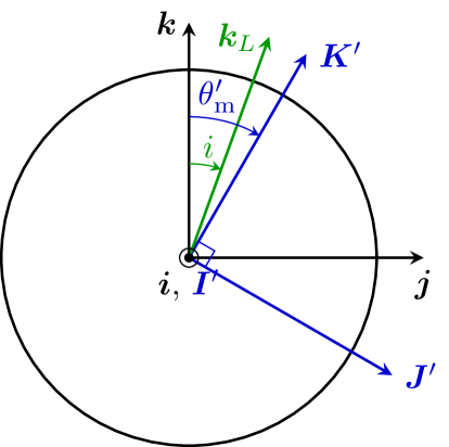
Figure 1: Sign convention. $\vec{k}_{L}$ is the normal of the invariant plane, $(\vec{I}^{\prime},\vec{J}^{\prime},\vec{K}^{\prime})$ is a frame attached to the mantle and $(\vec{i},\vec{j},\vec{k})$ is the orbit frame. When $\vec{k}$, $\vec{k}_{L}$ and $\vec{K}^{\prime}$ are coplanar (Cassini’s third law), the orbital inclination $i$ and the obliquity $\theta^{\prime}_{\mathrm{m}}$ are taken positive in the clockwise direction as illustrated in this figure. The same convention applies for the tilt angle of the core spin-axis $\theta^{\prime}_{\mathrm{c}}$.

The conditions for the system to be in a Cassini state can be written in terms of $\theta^{\prime}_{\rm m}$ and $\theta^{\prime}_{\rm c}$ only. In that scope, we notice from Eq. (32a) that

$$\langle\vec{K}^{\prime},\vec{\pi}^{\prime}_{\rm m}\rangle=C_{\rm m}\big{(}g\langle\vec{K}^{\prime},\vec{k}_{L}\rangle+\omega_{p}\big{)}\,,\qquad[\vec{K}^{\prime},\vec{\pi}^{\prime}_{\rm m}]={\rm I}_{\rm m}\left(1-\frac{1}{3}\alpha_{\rm m}\right)g[\vec{K}^{\prime},\vec{k}_{L}]\,,$$ (33)

where we used $C_{\rm m}={\rm I}_{\rm m}(1+\frac{2}{3}\alpha_{\rm m})$ (see Appendix A). Equalities (33) allow to get rid of $\vec{\pi}^{\prime}_{\rm m}$ in Eqs. (32b, 32c). At first order in $\alpha_{\rm c}$, the constraint $[\partial\bar{H}^{\prime}_{0}/\partial\vec{\pi}^{\prime}_{\rm c},\vec{\pi}^{\prime}_{\rm c}]=\vec{0}$ provides

$$\alpha_{\rm c}\omega_{p}\cos(\theta^{\prime}_{\rm m}-\theta^{\prime}_{\rm c})\sin(\theta^{\prime}_{\rm m}-\theta^{\prime}_{\rm c})+g\sin(i-\theta^{\prime}_{\rm c})=0\;.$$ (34a)

In the calculation of $$\hat{\mathcal{J}}^{\prime}(\bar{H}^{\prime}_{0}) [\vec{Y}_{2m},\vec{Y}_{2k}] \hat{\mathcal{J}}^{\prime}(\bar{H}^{\prime}_{0}) \vec{i}$$, the spherical harmonic matrices are rotated according to Eqs. (11) and the commutators are taken from the multiplication table 1. A direct calculation shows that is proportional to the matrix . Equating the coefficient to zero, we get at first order in flattening coefficients:

$$\begin{split}&-\alpha_{\rm c}C_{\rm c}\omega_{p}^{2}\cos(\theta^{\prime}_{\rm m}-\theta^{\prime}_{\rm c})\sin(\theta^{\prime}_{\rm m}-\theta^{\prime}_{\rm c})\\ &-\frac{3}{2}\frac{\mathcal{G}m_{0}}{a^{3}}C\left(\alpha X_{0}^{-3,0}(e)\cos\theta^{\prime}_{\rm m}\sin\theta^{\prime}_{\rm m}+\frac{1}{4}\beta X_{2p}^{-3,2}(e)(1+\cos\theta^{\prime}_{\rm m})\sin\theta^{\prime}_{\rm m}\right)\\ &-C_{\rm m}g\omega_{p}\sin(\theta^{\prime}_{\rm m}-i)=0.\end{split}$$ (34b)

At this stage, it is time to mark a pause to interpret the different terms of Eqs. (34b) which must be fulfilled by $\theta^{\prime}_{\rm m}$ and $\theta^{\prime}_{\rm c}$ for the system to be at equilibrium. First of all, the last two lines of Eq. (34b) are exactly those obtained by Peale (1969, eq. 18) for a rigid body. Thus in absence of coupling between the layers, i.e., when the core is spherical ($\alpha_{\rm c}=0$), the mantle behaves like a rigid planet or satellite as a whole but as if the precession frequency was reduced by a factor $C_{\rm m}/C$. The remaining term in the first line of Eq. (34b) represents the core-mantle coupling. Physically, this is a pressure torque coming from the rotation of the liquid core. Within the formalism of the present work, this term comes from the kinetic energy of rotation of the core. Finally, Eq. (34a) links the pressure torque exerted on the rigid mantle to the inertial torque induced by the rotating frame. According to this latter equation, if $\alpha_{\rm c}\rightarrow 0$, then $\sin(i-\theta^{\prime}_{\rm c})\rightarrow 0$. Therefore, in this case the angular momentum of the core tend to be aligned with the normal $\vec{k}_{L}$ of the Laplace plane and is either prograde ($\theta^{\prime}_{\rm c}=i$) or retrograde ($\theta^{\prime}_{\rm c}=i+\pi$).

To simplify a little Eqs. (34b), we apply Kepler’s third law $n^{2}a^{3}={\cal G}(m_{0}+M)$ and make the approximation $\omega_{p}\approx pn$. After some rearrangements, we get

$$p\alpha_{\rm c}\cos(\theta^{\prime}_{\rm m}-\theta^{\prime}_{\rm c})\sin(\theta^{\prime}_{\rm m}-\theta^{\prime}_{\rm c})+\frac{g}{n}\sin(i-\theta^{\prime}_{\rm c})=0\;,$$ (35a)

and

$$\begin{split}&\frac{3}{2p}\frac{m_{0}}{m_{0}+M}\frac{n}{g}\left(\alpha X_{0}^{-3,0}(e)\cos\theta^{\prime}_{\rm m}\sin\theta^{\prime}_{\rm m}+\frac{1}{4}\beta X_{2p}^{-3,2}(e)(1+\cos\theta^{\prime}_{\rm m})\sin\theta^{\prime}_{\rm m}\right)\\ &+\frac{C_{\rm m}}{C}\sin(\theta^{\prime}_{\rm m}-i)+\left(1-\frac{C_{\rm m}}{C}\right)\sin(\theta^{\prime}_{\rm c}-i)=0\;.\end{split}$$ (35b)

This set of equations (35) is in agreement with Eqs. (19-21) of (Stys and Dumberry, 2018) when the moments of inertia of the rigid core in ibid are set to zero. In conclusion, the position of the Cassini states are function of eight parameters: the dynamical flattening coefficients of the whole body $\alpha$, $\beta$, the polar flattening coefficient of the core $\alpha_{\rm c}$, the polar moment of inertia ratio $C_{\rm m}/C$, the eccentricity $e$, the inclination $i$, the nodal precession frequency in units of mean motion $g/n$, and the resonance number $p$. For cases of interest in the solar system, $p$ is either equal to 1 (synchronous rotation as for the Moon and for most regular satellites of the giant planets) or to $3/2$ ($3\!:\!2$ spin-orbit resonance like Mercury). The associated Hansen coefficients are

$$X_{0}^{-3,0}(e)=(1-e^{2})^{-3/2}\,,$$ (36a)

$$X_{2}^{-3,2}(e)=1-\frac{5}{2}e^{2}+\frac{13}{16}e^{4}+O(e^{6})\,,\qquad(p=1)\,,$$ (36b)

$$X_{3}^{-3,2}(e)=\frac{7}{2}e-\frac{123}{16}e^{3}+\frac{489}{128}e^{5}+O(e^{7})\,,\qquad(p=3/2)\,.$$ (36c)

Notice that in situations where the rotation speed is not in resonance with the orbital mean motion ($p$ is not a half integer), $X_{2p}^{-3,2}(e)$ has to be set to zero in Eq. (35b).

5 Cassini states: stability

To assert the stability of the Cassini states, we shall linearise the equations of motion in their vicinity. To do so, we parametrise the state of the system $(\vec{\pi}^{\prime}_{\rm m},\vec{\pi}^{\prime}_{\rm c},\vec{R}^{\prime})$ by a set of 8 coordinates $y^{\prime}=(\pi^{\prime}_{{\rm m},x},\pi^{\prime}_{{\rm m},y},\pi^{\prime}_{{\rm m},z},\phi^{\prime}_{\rm c},\theta^{\prime}_{\rm c},\phi^{\prime}_{\rm m},\theta^{\prime}_{\rm m},\psi^{\prime}_{\rm m})\in\mathbb{R}^{8}$ where $(\pi^{\prime}_{{\rm m},x},\pi^{\prime}_{{\rm m},y},\pi^{\prime}_{{\rm m},z})$ are the Cartesian coordinates of the mantle angular momentum, where $(\phi^{\prime}_{\rm m},\theta^{\prime}_{\rm m},\psi^{\prime}_{\rm m})$ are the Euler (3,-1,3) angles defining the rotation matrix $\vec{R}^{\prime}$ (i.e., $\vec{R}^{\prime}=\vec{R}_{3}(\phi^{\prime}_{\rm m})\vec{R}_{1}(-\theta^{\prime}_{\rm m})\vec{R}_{3}(\psi^{\prime}_{\rm m})$) and where $(\phi^{\prime}_{\rm c},\theta^{\prime}_{\rm c})$ are defined in such a way that $\hat{\vec{\pi}}^{\prime}_{\rm c}=\hat{\mathcal{R}}_{3}(\phi^{\prime}_{\rm c})\circ\hat{\mathcal{R}}_{1}(-\theta^{\prime}_{\rm c})\,[\vec{k}]$. Within this choice of variables, Cassini states are located in the subspace $\phi^{\prime}_{\rm c}=\phi^{\prime}_{\rm m}=\psi^{\prime}_{\rm m}=0$ and ($\theta^{\prime}_{\rm m},\theta^{\prime}_{\rm c}$) have the same meaning as in the previous section, i.e., they correspond to the obliquities of the two layers with the same sign convention as in Peale (1969).

Let $y^{\prime}_{e}$ be a fixed point of the averaged problem (i.e., the coordinates of a Cassini state), then $y^{\prime}_{e}$ is solution of $\nabla_{y^{\prime}}\bar{H}^{\prime}_{0}(y^{\prime}_{e})=0$. The equations of motion are $\dot{y}^{\prime}=-B(y^{\prime})\nabla_{y^{\prime}}\bar{H}^{\prime}_{0}(y^{\prime})$ where $B(y^{\prime})$ is a Poisson matrix (provided below), therefore the linearised equations of motion in the vicinity of $y^{\prime}_{e}$ are of the form

$$\dot{y}^{\prime}=A(y-y^{\prime}_{e})\;,\qquad A=-B(y^{\prime}_{e})\nabla^{2}_{y^{\prime}}\bar{H}^{\prime}_{0}(y^{\prime}_{e})\;.$$ (37)

5.1 Hessian of the Hamiltonian

To get the Hessian $\nabla^{2}_{y^{\prime}}\bar{H}^{\prime}_{0}$ of the Hamiltonian $\bar{H}^{\prime}_{0}$ (30a), we compute its second variation $\delta^{2}\bar{H}^{\prime}_{0}$ which is a quadratic form in $\delta y^{\prime}=(\delta\pi^{\prime}_{{\rm m},x},\delta\pi^{\prime}_{{\rm m},y},\delta\pi^{\prime}_{{\rm m},z},\delta\phi^{\prime}_{\rm c},\delta\theta^{\prime}_{\rm c},\delta\phi^{\prime}_{\rm m},\delta\theta^{\prime}_{\rm m},\delta\psi^{\prime}_{\rm m})$. The Hessian is then the symmetric matrix of this quadratic form. To calculate $\delta^{2}\bar{H}^{\prime}_{0}$, we use the fact it is a function of several quantities $(\vec{\pi}^{\prime}_{\rm c},\vec{K}^{\prime},\vec{Y}^{\prime}_{2m})$ varying under rotation only. In that scope, we parametrise any infinitesimal rotation $\delta\vec{R}$ relative to a given rotation $\vec{R}$ by an element of the respective Lie algebra $\delta\vec{\Theta}\coloneqq\delta\vec{R}\,{\vec{R}}^{\mathrm{T}}$. To the orientation of the core angular momentum $\vec{\pi}^{\prime}_{\rm c}$, represented by the rotation matrix $\vec{R}_{3}(\phi^{\prime}_{\rm c})\vec{R}_{1}(-\theta^{\prime}_{\rm c})$, we associate the element

$$\delta\vec{\Theta}^{\prime}_{\rm c}=\delta\phi^{\prime}_{\rm c}\vec{k}-\delta\theta^{\prime}_{\rm c}\vec{i}^{\prime}_{\rm c}\,,$$ (38a)

and for the rotation matrix $$\vec{R}^{\prime}=\vec{R}_{3}(\phi^{\prime}_{\rm m})\vec{R}_{1}(-\theta^{\prime}_{\rm m})\vec{R}_{3}(\psi^{\prime}_{\rm m})$$ we define

$$\delta\vec{\Theta}^{\prime}_{\rm m}=\delta\phi^{\prime}_{\rm m}\vec{k}-\delta\theta^{\prime}_{\rm m}\vec{i}^{\prime}_{\rm m}+\delta\psi^{\prime}_{\rm m}\vec{K}^{\prime}\;.$$ (38b)

In these equations, $$\vec{i}^{\prime}_{\lambda}={\hat{\mathcal{R}}}_{3}(\phi^{\prime}_{\lambda})[\vec{i}] \lambda\in\{{\rm m},{\rm c}\} \vec{K}^{\prime}=\hat{\mathcal{R}}_{3}(\phi^{\prime}_{\rm m})\circ\hat{\mathcal{R}}_{1}(-\theta^{\prime}_{\rm m})\,[\vec{k}] \vec{i}^{\prime}_{\rm m}=\vec{i}^{\prime}_{\rm c}=\vec{i} \vec{K}^{\prime}=\hat{\mathcal{R}}_{1}(-\theta^{\prime}_{\rm m})[\vec{k}] \delta^{2}\bar{H}^{\prime}_{0}$$, , and . In particular, when the system is in a Cassini state, and . In the derivation of , the second variation of the rotation matrices are also required. We have

$$\delta^{2}\vec{\Theta}^{\prime}_{\rm c}=-\delta\phi^{\prime}_{\rm c}\delta\theta^{\prime}_{\rm c}\,[\vec{k},\vec{i}^{\prime}_{\rm c}]\,,$$ (38c)

$$\delta^{2}\vec{\Theta}^{\prime}_{\rm m}=-\delta\phi^{\prime}_{\rm m}\delta\theta^{\prime}_{\rm m}\,[\vec{k},\vec{i}^{\prime}_{\rm m}]+\delta\phi^{\prime}_{\rm m}\delta\psi^{\prime}_{\rm m}\,[\vec{k},\vec{K}^{\prime}]-\delta\theta^{\prime}_{\rm m}\delta\psi^{\prime}\,[\vec{i}^{\prime}_{\rm m},\vec{K}^{\prime}]\,.$$ (38d)

With these quantities being defined, the first variations of $(\vec{\pi}^{\prime}_{\rm c},\vec{K}^{\prime},\vec{Y}^{\prime}_{2m})$ are given by

$$\delta\vec{\pi}^{\prime}_{\rm c}=[\delta\vec{\Theta}^{\prime}_{\rm c},\vec{\pi}^{\prime}_{c}]\,,$$ (39a)

$$\delta\vec{K}^{\prime}=[\delta\vec{\Theta}^{\prime}_{\rm m},\vec{K}^{\prime}]\,,$$ (39b)

$$\delta\vec{Y}^{\prime}_{2m}=[\delta\vec{\Theta}^{\prime}_{\rm m},\vec{Y}^{\prime}_{2m}]\,,$$ (39c)

and their second variations by

$$\delta^{2}\vec{\pi}^{\prime}_{\rm c}=[\delta^{2}\vec{\Theta}^{\prime}_{\rm c},\vec{\pi}^{\prime}_{\rm c}]+[\delta\vec{\Theta}^{\prime}_{\rm c},\delta\vec{\pi}^{\prime}_{\rm c}]\,,$$ (39d)

$$\delta^{2}\vec{K}^{\prime}=[\delta^{2}\vec{\Theta}^{\prime}_{\rm m},\vec{K}^{\prime}]+[\delta\vec{\Theta}^{\prime}_{\rm m},\delta\vec{K}^{\prime}]\,,$$ (39e)

$$\delta^{2}\vec{Y}^{\prime}_{2m}=[\delta^{2}\vec{\Theta}^{\prime}_{\rm m},\vec{Y}^{\prime}_{2m}]+[\delta\vec{\Theta}^{\prime}_{\rm m},\delta\vec{Y}^{\prime}_{2m}]\,.$$ (39f)

As for the angular momentum of the mantle, we have

$$\delta\vec{\pi}^{\prime}_{\rm m}=\delta\pi^{\prime}_{{\rm m},x}\,\vec{i}+\delta\pi^{\prime}_{{\rm m},y}\,\vec{j}+\delta\pi^{\prime}_{{\rm m},z}\,\vec{k}\,,\qquad\delta^{2}\vec{\pi}^{\prime}_{{\rm m}}=\vec{0}\,.$$ (40)

Furthermore, the Hamiltonian (30a) depends on the above variables through scalar products and for any function $f=\langle\vec{A},\vec{B}\rangle$, we have

$$\delta f=\langle\delta\vec{A},\vec{B}\rangle+\langle\vec{A},\delta\vec{B}\rangle\,,\qquad\delta^{2}f=\langle\delta^{2}\vec{A},\vec{B}\rangle+2\langle\delta\vec{A},\delta\vec{B}\rangle+\langle\vec{A},\delta^{2}\vec{B}\rangle\,,$$ (41a)

and

$$\delta\left(f^{2}\right)=2f\delta f\,,\qquad\delta^{2}\left(f^{2}\right)=2\left(\delta f\right)^{2}+2f\left(\delta^{2}f\right)\,.$$ (41b)

The calculation of $\delta^{2}\bar{H}^{\prime}_{0}$ has been implemented in TRIP, a general computer algebra system dedicated to celestial mechanics (Gastineau and Laskar, 2011).

5.2 Poisson matrix

To get the Poisson matrix $B(y^{\prime})$ in the variables $y^{\prime}$ reproducing the equations of motion (18), we shall first determine the expression of the spin operator $\hat{\mathcal{J}}^{\prime}$. In this section, we rather consider its vector counterpart $\hat{J}^{\prime}$ (i.e., whose image is in $\mathbb{R}^{3}$). Let $y^{\prime}_{\rm m}=(\phi^{\prime}_{\rm m},\theta^{\prime}_{\rm m},\psi^{\prime}_{\rm m})$ and $\mathsf{J}^{\prime}(y^{\prime}_{\rm m})$ the matrix such that

$$\hat{J}^{\prime}(\bar{H}^{\prime}_{0})=\mathsf{J}^{\prime}(y^{\prime}_{\rm m})\frac{\partial\bar{H}^{\prime}_{0}}{\partial y^{\prime}_{\rm m}}\,.$$ (42)

By construction, $\mathsf{J}^{\prime}(y^{\prime}_{\rm m})$ also satisfies (see Boué and Efroimsky, 2019)

$$\delta\vec{\Theta}^{\prime}_{\rm m}=\left({\mathsf{J}^{\prime}(y^{\prime}_{\rm m})}^{\mathrm{T}}\right)^{-1}\delta y^{\prime}_{\rm m}\,,$$ (43)

where $\delta\vec{\Theta}^{\prime}_{\rm m}$ is the 3D vector representing the skew-symmetric matrix $\delta\vec{\Theta}^{\prime}_{\rm m}$. Based on Eq. (38b), we get

$$\delta\vec{\Theta}^{\prime}_{\rm m}=\begin{pmatrix}-\delta\theta^{\prime}_{\rm m}\cos\phi^{\prime}_{\rm m}-\delta\psi^{\prime}_{\rm m}\sin\theta^{\prime}_{\rm m}\sin\phi^{\prime}_{\rm m}\\ -\delta\theta^{\prime}_{\rm m}\sin\phi^{\prime}_{\rm m}+\delta\psi^{\prime}_{\rm m}\sin\theta^{\prime}_{\rm m}\cos\phi^{\prime}_{\rm m}\\ \delta\phi^{\prime}_{\rm m}+\delta\psi^{\prime}_{\rm m}\cos\theta^{\prime}_{\rm m}\end{pmatrix}\,,$$ (44)

and by identification of the last two equations, we obtain

$$\mathsf{J}^{\prime}(y^{\prime}_{\rm m})=\begin{bmatrix}\cot\theta^{\prime}_{\rm m}\sin\phi^{\prime}_{\rm m}&&-\cos\phi^{\prime}_{\rm m}&&-\csc\theta^{\prime}_{\rm m}\sin\phi^{\prime}_{\rm m}\\ -\cot\theta^{\prime}_{\rm m}\cos\phi^{\prime}_{\rm m}&&-\sin\phi^{\prime}_{\rm m}&&\csc\theta^{\prime}_{\rm m}\cos\phi^{\prime}_{\rm m}\\ 1&&0&&0\end{bmatrix}\ .$$ (45)

The first three lines of the Poisson matrix provide the evolution rate of $\vec{\pi}^{\prime}_{\rm m}$. From Eq. (18a), we have $\!\!\dot{\ \ \vec{\pi}^{\,\prime}_{\rm m}}=-\vec{\pi}^{\prime}_{\rm m}\times({\partial H^{\prime}_{0}}/{\partial\vec{\pi}^{\prime}_{\rm m}})-\hat{J}^{\prime}(\bar{H}^{\prime}_{0})$. As a result, the first three lines of the Poisson matrix are

$$\begin{bmatrix}0&-\pi^{\prime}_{{\rm m},z}&\pi^{\prime}_{{\rm m},y}&0&0&\cot\theta^{\prime}_{\rm m}\sin\phi^{\prime}_{\rm m}&-\cos\phi^{\prime}_{\rm m}&-\csc\theta^{\prime}_{\rm m}\sin\phi^{\prime}_{\rm m}\\[1.99997pt] \pi^{\prime}_{{\rm m},z}&0&-\pi^{\prime}_{{\rm m},x}&0&0&-\cot\theta^{\prime}_{\rm m}\cos\phi^{\prime}_{\rm m}&-\sin\phi^{\prime}_{\rm m}&\csc\theta^{\prime}_{\rm m}\cos\phi^{\prime}_{\rm m}\\[1.99997pt] -\pi^{\prime}_{{\rm m},y}&\pi^{\prime}_{{\rm m},x}&0&0&0&1&0&0\end{bmatrix}\,.$$ (46)

As for the last three lines of the Poisson matrix, we write the time derivative of $y^{\prime}_{\rm m}$ in terms of $\vec{\omega}^{\prime}_{\rm m}$ deduced from Eq. (43), namely,

$$\dot{y}^{\prime}_{\rm m}={\mathsf{J}^{\prime}(y^{\prime}_{\rm m})}^{\mathrm{T}}\,\vec{\omega}^{\prime}_{\rm m}\,,$$ (47)

with $\vec{\omega}_{\rm m}=\partial H^{\prime}_{0}/\partial\vec{\pi}^{\prime}_{\rm m}$. Therefore, the last three lines of the Poisson matrix are

$$\begin{bmatrix}-\cot\theta^{\prime}_{\rm m}\sin\phi^{\prime}_{\rm m}&\cot\theta^{\prime}_{\rm m}\cos\phi^{\prime}_{\rm m}&-1&0&0&0&0&0\\ \cos\phi^{\prime}_{\rm m}&\sin\phi^{\prime}_{\rm m}&0&0&0&0&0&0\\ \csc\theta^{\prime}_{\rm m}\sin\phi^{\prime}_{\rm m}&-\csc\theta^{\prime}_{\rm m}\cos\phi^{\prime}_{\rm m}&0&0&0&0&0&0\end{bmatrix}\,.$$ (48)

Finally, to get the entire Poisson matrix, we add the part governing the evolution of the orientation of the core angular momentum $(\phi^{\prime}_{\rm c},\theta^{\prime}_{\rm c})$. In that scope, we apply the derivation chain rule. The result is

$$B(y^{\prime})=\begin{bmatrix}0&-\pi^{\prime}_{{\rm m},z}&\pi^{\prime}_{{\rm m},y}&0&0&\displaystyle\frac{\sin\phi^{\prime}_{\rm m}}{\tan\theta^{\prime}_{\rm m}}&-\cos\phi^{\prime}_{\rm m}&\displaystyle-\frac{\sin\phi^{\prime}_{\rm m}}{\sin\theta^{\prime}_{\rm m}}\\[10.00002pt] \pi^{\prime}_{{\rm m},z}&0&-\pi^{\prime}_{{\rm m},x}&0&0&\displaystyle-\frac{\cos\phi^{\prime}_{\rm m}}{\tan\theta^{\prime}_{\rm m}}&-\sin\phi^{\prime}_{\rm m}&\displaystyle\frac{\cos\phi^{\prime}_{\rm m}}{\sin\theta^{\prime}_{\rm m}}\\[10.00002pt] -\pi^{\prime}_{{\rm m},y}&\pi^{\prime}_{{\rm m},x}&0&0&0&1&0&0\\[1.99997pt] 0&0&0&0&\displaystyle\frac{1}{\pi_{c}\sin\theta^{\prime}_{\rm c}}&0&0&0\\ 0&0&0&\displaystyle-\frac{1}{\pi_{c}\sin\theta^{\prime}_{\rm c}}&0&0&0&0\\ \displaystyle-\frac{\sin\phi^{\prime}_{\rm m}}{\tan\theta^{\prime}_{\rm m}}&\displaystyle\frac{\cos\phi^{\prime}_{\rm m}}{\tan\theta^{\prime}_{\rm m}}&-1&0&0&0&0&0\\[10.00002pt] \cos\phi^{\prime}_{\rm m}&\sin\phi^{\prime}_{\rm m}&0&0&0&0&0&0\\[3.99994pt] \displaystyle\frac{\sin\phi^{\prime}_{\rm m}}{\sin\theta^{\prime}_{\rm m}}&\displaystyle-\frac{\cos\phi^{\prime}_{\rm m}}{\sin\theta^{\prime}_{\rm m}}&0&0&0&0&0&0\end{bmatrix}\,.$$ (49)

We verify that the so-constructed Poisson matrix is skew-symmetric as it should be.

5.3 Stability criterion

A fixed point $y^{\prime}_{e}$ is said to be Lyapunov stable if the Hessian $\nabla^{2}_{y^{\prime}}\bar{H}^{\prime}_{0}(y^{\prime}_{e})$ is positive definite (all eigenvalues are strictly positive) or negative definite (all eigenvalues are strictly negative). The kinetic part of the Hamiltonian guarantees positive eigenvalues and Lyapunov stable equilibria are de facto associated with a positive definite Hessian. Besides the Lyapunov stability criterion, which is a strong criterion hardly satisfied in our problem (see Appendix C.2), we also consider spectral stability which states that a fixed point $y^{\prime}_{e}$ is stable if all the (complex) eigenvalues of the matrix $A$ of the linearised system (37) are purely imaginary (no real part). Lyapunov stability implies spectral stability but the converse is not true. To estimate the impact of dissipation (not included here) on these two types of stability, we refere the reader to the comprehensive review by Krechetnikov and Marsden (2007).

6 Results

6.1 Application to Mercury

In this section we analyse Mercury’s possible Cassini states predicted by the present idealised model according to which the core is a perfect fluid undergoing Poincaré’s simple motion and the mantle is totally rigid. The physical and orbital parameters, summarised in Table 2, are mainly taken from (Baland et al., 2017). The exceptions are the polar moment of inertia ratio $C_{\rm m}/C$ provided by (Smith et al., 2012) and the polar flattening of the core $\alpha_{\rm c}$ which we allow to vary between 0 and $\alpha$.

Table 2: Mercury’s parameters.

Parameter	Symbol	Value	Reference
planet polar flattening coefficient	$\alpha$	$0.14658\times 10^{-3}$	(Baland et al., 2017)
planet equatorial flattening coefficient	$\beta$	$0.93666\times 10^{-4}$	(Baland et al., 2017)
core polar flattening coefficient	$\alpha_{\rm c}/\alpha$	from $\,0\,$ to 1
polar moment of inertia ratio	$C_{\rm m}/C$	$0.452$	(Smith et al., 2012)
orbital eccentricity	$e$	$0.20563$	(Baland et al., 2017)
orbital inclination	$i$	$8.533^{\circ}$	(Baland et al., 2017)
precession frequency in units of mean motion	$g/n$	$-0.73990\times 10^{-6}$	(Baland et al., 2017)
resonance	$p$	$3/2$
planet-to-Sun mass ratio	$M/m_{0}$	neglected

To get the location of Mercury’s Cassini states, the system (35) is written as a set of polynomial equations in $\left\{X_{\rm m}=\cos\theta^{\prime}_{\rm m},\,Y_{\rm m}=\sin\theta^{\prime}_{\rm m},\,X_{\rm c}=\cos\theta^{\prime}_{\rm c},\,Y_{\rm c}=\sin\theta^{\prime}_{\rm c}\right\}$ to which the conditions $X_{\rm m}^{2}+Y_{\rm m}^{2}=1$ and $X_{\rm c}^{2}+Y_{\rm c}^{2}=1$ are added. The polynomial system is solved using the command Isolate of Maple’s package RootFinding. The spectral stability of each solution is determined using TRIP as described in Section 5. Results are displayed in Figure 2 as a function of $\alpha_{\rm c}/\alpha$. Several remarkable points deserve to be commented.

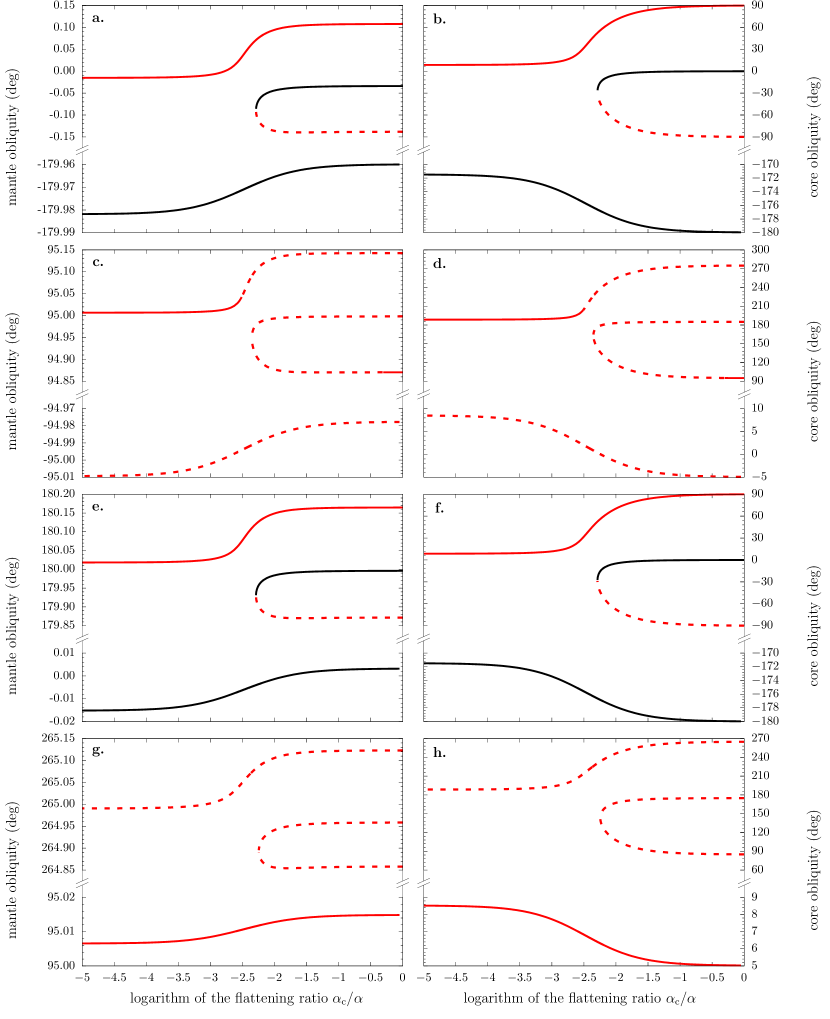
Figure 2: Mercury’s Cassini states as a function of $\log_{10}(\alpha_{\rm c}/\alpha)$. Each row displays the location of a given set of fixed point families projected onto $\theta^{\prime}_{\rm m}$: mantle obliquity (left panel) and $\theta^{\prime}_{\rm c}$: core obliquity (right panel). The spectral and Lyapunov stabilities of each Cassini states are determined as described in Sect. 5: Lyapunov stable equilibria are represented with solid black curves, spectral stable but Lyapunov unstable ones are plotted with solid red curves, unstable ones are displayed with red dashed curves.

There exists up to 16 different equilibrium solutions. By comparison, a completely rigid body only possesses at most 4 stationary states (Colombo, 1966; Peale, 1969). The solutions presented in Fig. 2a and 2b actually behave like the 4 Cassini states of the classical problem (e.g., Ward and Hamilton, 2004, fig. 3). Up to a critical value of the varying parameter (here $\alpha^{\rm crit}_{\rm c}\approx 10^{-2.3}\alpha\approx 0.005\,\alpha$) there are two elliptical fixed points (solid curves): one prograde close to $0^{\circ}$ of obliquity and the other retrograde near $180^{\circ}$. At $\alpha_{\rm c}=\alpha^{\rm crit}_{\rm c}$ a double fixed point appears. For $\alpha_{\rm c}>\alpha^{\rm crit}_{\rm c}$, the latter bifurcates into two prograde equilibria, one being stable (solid black) and the other unstable (dashed red). We also notice that the bifurcation pattern of the core is significantly more widened than that of the mantle. Whereas the latter obliquity is bounded between $-0.15^{\circ}$ and $0.10^{\circ}$, the core can be tilted up to $\pm 90^{\circ}$. Let us emphasise another important point: the Cassini state ranging from $\sim 0^{\circ}$ to $\sim 0.10^{\circ}$ is spectrally stable but Lyapunov unstable (solid red curve). This results is quite puzzling because the Moon actually is in this state (see Section 6.2). Nevertheless, in Appendix C.2 we show that this Lyapunov instability is also predicted in the much more simple Colombo’s top model. We thus conclude that the Lyapunov stability criterion is too restrictive for our problem and hereafter only consider the spectral stability.

The bifurcation pattern shown in the upper half of Fig. 2a is reproduced three times around $\theta^{\prime}_{\rm m}=95^{\circ}$ (Fig. 2c), $180^{\circ}$ (Fig. 2e), and $265^{\circ}$ (Fig. 2g). Moreover, to each of these equilibrium solutions, there exists an isolated curve of fixed points diametrically opposite, i.e., offset by $180^{\circ}$ (lower half of Figs. 2a,c,e,g). Nevertheless there are discrepancies between the first and the last three rows of Fig. 2. In the latter, the bifurcation pattern of the core is offset from that of the mantle by the order of $90^{\circ}$ or $180^{\circ}$. Therefore, at these new Cassini states, the core is significantly tilted from the mantle (except for very specific values of the parameter $\alpha_{\rm c}$). Additionally, the spectral stabilities are not alike in all rows. In the second and fourth rows, we observe bifurcations with the appearance of two hyperbolic fixed points. Moreover, along a same family of fixed point, the stability happens to switch from stable to unstable and vice versa (Figs. 2c and 2d).

When $\alpha_{\rm c}\rightarrow 0$ the core is decoupled from the mantle (see Eqs. 35). Therefore, the latter must behave like a rigid body and cannot have more than four different Cassini states. This is indeed the case. The four equilibrium obliquities of the mantle in the limit $\alpha_{\rm c}\rightarrow 0$ are $\theta^{\prime}_{\rm m}=-0.02^{\circ}$ and $180.02^{\circ}$ (Figs. 2a and 2e), and $\theta^{\prime}_{\rm m}=\pm 95.01^{\circ}$ (Figs. 2c and 2g). Moreover, only one of these fixed points is unstable (the one at $\theta^{\prime}_{\rm m}=-95.01^{\circ}$). At each of these four fixed points, the core obliquity takes two different values, namely $i=8.533^{\circ}$ and $i+\pi=188.533^{\circ}$, as explained in Sect. 4.

In the limit $\alpha_{\rm c}\rightarrow\alpha$, the solution with the lowest obliquity in Figs. 2a and 2b is at $\theta^{\prime}_{\rm m}\approx-0.034^{\circ}$ and $\theta^{\prime}_{\rm c}\approx-0.067^{\circ}$. It is remarkable that for this particular Cassini states, the core and the mantle are almost aligned. Therefore, the mantle obliquity is close to the value obtained when assuming the planet to be completely rigid, namely $2.05\,{\rm arcmin}=0.034^{\circ}$ (e.g., Baland et al., 2017).

6.2 Low obliquity Cassini states

Here we focus on the low obliquity Cassini states of Mercury, the Moon and Io. We choose these bodies in particular because they all have been described by a model with a liquid core in the literature. Physical and orbital parameters of Mercury are provided in Table 2, those of the Moon and Io are displayed in Table 3.

Table 3: Parameters of the Moon and Io.

Parameter	Symbol	Moon	Io
body polar flattening coefficient	$\alpha$	$0.51690\times 10^{-3\;{\rm a}}$	$4.8982\times 10^{-3\;\rm c}$
body equatorial flattening coefficient	$\beta$	$0.22772\times 10^{-3\;{\rm a}}$	$5.8770\times 10^{-3\;\rm c}$
core polar flattening coefficient	$\alpha_{\rm c}/\alpha$	from $\,0\,$ to 1	from $\,0\,$ to 1
polar moment of inertia ratio	$C_{\rm m}/C$	$0.9993^{\;\rm a}$	$0.98346^{\;\rm d}$
orbital eccentricity	$e$	$0.0549^{\,\rm b}$	$0.00415^{\;\rm e}$
orbital inclination	$i$	$5.145^{\circ\;{\rm b}}$	$0.036^{\circ\;\rm e}$
precession frequency in units of mean motion	$g/n$	$-0.40188\times 10^{-2\;\rm b}$	$-0.62832\times 10^{-3\;\rm e}$
resonance	$p$	$1$	$1$
body-to-central mass ratio	$M/m_{0}$	$0.0123^{\;\rm a}$	neglected

^a (Viswanathan et al., 2017);  ^b (Yoder, 1995);  ^c (Anderson et al., 2001);  ^d (Noyelles, 2014, , Section 4.4, model 1);  ^e (Lainey et al., 2006)

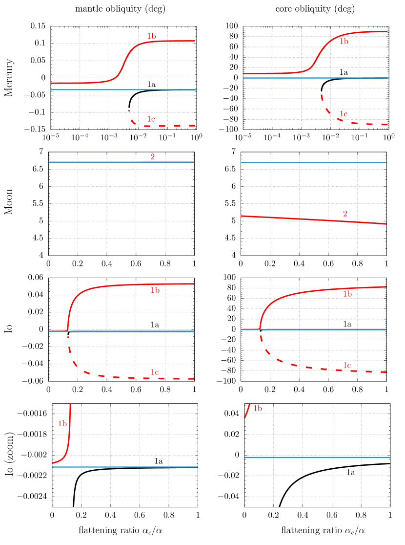
Figure 3: Cassini states labelled ‘1a’, ‘1b’, ‘1c’, ‘2’ as a function of $\alpha_{\rm c}/\alpha$. black solid curve: spectral and Lyapunov stable points, red solid curves: spectral stable but Lyapunov unstable points, red dashed curve: spectral unstable points, blue solid curve: solution of the fully rigid model (Peale, 1969). Top row: Mercury’s Cassini states, second row: Moon’s Cassini states, third row: Io’s Cassini states, bottom row: zoom on Io’s Cassini states.

The location and stability of the Cassini states are computed as described in Sect. 4 and 5. These positions are then compared with those expected from a fully rigid model (Peale, 1969) in Fig. 3. According to the standard rigid body nomenclature of Cassini states (Peale, 1969), Mercury and Io are lying on state 1 (the stable branch arising from the bifurcation) while the Moon is settled on state 2 (the prograde branch extending over the whole parameter space). From Figure 3, we observe that for the present values of the Moon’s physical and orbital parameters, introducing a fluid core does not split the branch of Cassini states 2. The derived mantle obliquity is very close to that predicted by Peale’s formula and the core is only tilted by about 1.5^∘. In the case of Mercury and Io, however, the presence of a liquid core does break state 1 into three different branches labelled ‘1a’, ‘1b’ and ‘1c’ (see Fig. 3). For both these bodies, the branch ‘1a’ remain very close to the obliquity inferred from Peale’s model. When the core flattening coefficient is less than the minimal value required for the existence of states ‘1a’ and ‘1c’, the branch ‘1b’ is reasonably close the rigid body expectation. As explained in the previous section, the difference is a function of $C_{\rm m}/C$. It should be stressed that this offset which implies a departure from the observed obliquity (in the case of Mercury at least) does not preclude the existence of a spherical core. Indeed, a slight correction of the physical parameters would allow to recover the observed value. Finally, as the ratio $\alpha_{\rm c}/\alpha$ goes to 1, the physical validity of states ‘1a’ and ‘1c’ becomes questionable given the large tilt of the core rotation axis relative to the mantle’s figure axis that reaches 90^∘.

7 Conclusion

In this work, we determine the orientations and stabilities of the Cassini states of a rigid body with a liquid layer described by the Poincaré-Hough model. The analysis is performed in a non-canonical Hamiltonian formalism where variables are represented by matrices. The spin-orbit gravitational interaction is written in terms of spherical harmonic matrices. The latter have good mathematical properties allowing to conduct the calculation efficiently.

The problem has four degrees of freedom but the condition for the system to be in a Cassini state is reduced to a set of only two equations whose unknowns are the mantle obliquity $\theta_{\mathrm{m}}$ and the tilt angle of the core spin-axis $\theta_{\mathrm{c}}$. These equations are

$$p\alpha_{\rm c}\cos(\theta_{\rm m}-\theta_{\rm c})\sin(\theta_{\rm m}-\theta_{\rm c})+\frac{g}{n}\sin(i-\theta_{\rm c})=0\;,$$

and

$$\begin{split}&\frac{3}{2p}\frac{m_{0}}{m_{0}+M}\frac{n}{g}\left(\alpha X_{0}^{-3,0}(e)\cos\theta_{\rm m}\sin\theta_{\rm m}+\frac{1}{4}\beta X_{2p}^{-3,2}(e)(1+\cos\theta_{\rm m})\sin\theta_{\rm m}\right)\\ &+\frac{C_{\rm m}}{C}\sin(\theta_{\rm m}-i)+\left(1-\frac{C_{\rm m}}{C}\right)\sin(\theta_{\rm c}-i)=0\;.\end{split}$$

They depend on eight parameters, namely, the core polar flattening coefficient $\alpha_{c}$, the overall polar and equatorial flattening coefficients $\alpha$ and $\beta$, the polar moment of inertia ratio $C_{\mathrm{m}}/C$, the body to companion mass ratio $M/m_{0}$, the orbital inclination $i$ and eccentricity $e$, the nodal precession frequency and the rotation speed in units of orbital mean motion $g/n$ and $p$, respectively. If $p$ is not a half integer, the Hansen coefficient $X_{2p}^{-3,2}(e)$ has to be set to zero. For an evanescent core, i.e., when $C_{\mathrm{m}}\rightarrow C$, we retrieve the equation whose roots are the obliquities of the Cassini states of a fully rigid body.

We present the formulae allowing to determine the Lyapunov and spectral stabilities of these Cassini states. For this problem, the Lyapunov stability criterion is very stringent as it cannot guarantee the stability of the current state of the Moon. We explain this outcome on a simplified axisymmetric problem corresponding to Colombo’s top.

The model is applied to Mercury, Io and the Moon. For Mercury we highlight 16 different branches of Cassini states as a function of $\alpha_{\mathrm{c}}/\alpha$. Given that the problem has three more degrees of freedom than in the fully rigid body case, the phase space presents more complex features. In particular, we observe the appearance of two spectrally unstable families from a same bifurcation point or transitions from stable to unstable configurations along two families of fixed points. Among the 16 Cassini states, if $\alpha_{\mathrm{c}}$ is sufficiently close to $\alpha$, 8 of them can be spectrally stable. In the same limit, one of the Cassini states inferred by this model for each of the studied body is very closed to that predicted by the fully rigid model. In most of the other solutions, the core happens to be significantly tilted with respect to the mantle. These latter configurations might not survive core-mantle friction. This will be the subject of a future work.

Appendix A Flattening coefficients

Let $A\leq B\leq C$ be the principal moments of inertia of a given body. The polar and equatorial flattening coefficients $\alpha$ and $\beta$ are respectively defined as (Van Hoolst and Dehant, 2002)

$$\alpha=\frac{C-(A+B)/2}{C}\;,\qquad\beta=\frac{B-A}{C}\;.$$ (50)

We denote by $I=(A+B+C)/3$ the mean moment of inertia. The following relations holds

$$A=I\left(1-\frac{1}{3}\alpha-\frac{1}{2}\beta\right)\;,\qquad B=I\left(1-\frac{1}{3}\alpha+\frac{1}{2}\beta\right)\;,\qquad C=I\left(1+\frac{2}{3}\alpha\right)\;.$$ (51)

Appendix B Spin operator

Let $\vec{M}$ and $\vec{N}$ be two matrices and $\vec{M}^{\prime}=\vec{R}\vec{M}{\vec{R}}^{\mathrm{T}}$ where $\vec{R}$ is a rotation matrix. Under an infinitesimal rotation increment, $\delta\vec{R}=\delta\vec{\Theta}\vec{R}$, with $\delta\vec{\Theta}\in\mathrm{skew}(3)$, the matrix $\vec{M}^{\prime}$ is transformed according to

$$\vec{M}^{\prime}+\delta\vec{M}^{\prime}=(\vec{R}+\delta\vec{R})\vec{M}{(\vec{R}+\delta\vec{R})}^{\mathrm{T}}=\vec{M}^{\prime}+[\delta\vec{\Theta},\vec{M}^{\prime}]+O(|\delta\vec{\Theta}|^{2})\;.$$ (52)

Let $f=\langle\vec{M}^{\prime},\vec{N}\rangle$. Under the same infinitesimal rotation, the variation of $f$ is given by

$$\begin{split}\delta f&=\langle[\delta\vec{\Theta},\vec{M}^{\prime}],\vec{N}\rangle\\ &=\langle\delta\vec{\Theta}\vec{M}^{\prime},\vec{N}\rangle-\langle\vec{M}^{\prime}\delta\vec{\Theta},\vec{N}\rangle\\ &=\langle\delta\vec{\Theta},\vec{N}\vec{M}^{\prime\mathrm{T}}\rangle-\langle\delta\vec{\Theta},\vec{M}^{\prime\mathrm{T}}\vec{N}\rangle\\ &=\langle\delta\vec{\Theta},[\vec{N},\vec{M}^{\prime\mathrm{T}}]\rangle\;.\end{split}$$ (53)

But by definition, this variation $\delta f$ can also be written $\delta f=\langle\delta\vec{\Theta},\hat{\mathcal{J}}(f)\rangle.$ We thus deduce that $\hat{\mathcal{J}}(f)=-[\vec{M}^{\prime\mathrm{T}},\vec{N}]$. In particular, if $\vec{M}=\vec{S}$ is symmetric ($\vec{S}={\vec{S}}^{\mathrm{T}}$), then

$$\hat{\mathcal{J}}(\langle\vec{S}^{\prime},\vec{N}\rangle)=-[\vec{S}^{\prime},\vec{N}]\;,$$ (54)

while if $\vec{M}=\vec{A}$ is skew-symmetric ($\vec{A}=-{\vec{A}}^{\mathrm{T}}$),

$$\hat{\mathcal{J}}(\langle\vec{A}^{\prime},\vec{N}\rangle)=[\vec{A}^{\prime},\vec{N}]\;.$$ (55)

Appendix C Stability of Colombo’s top

Colombo’s top is an axisymmetric body whose orientation is determined by a single vector representing the direction of the figure axis. Both the kinetic and the potential energies can be expressed in terms of this vector. By consequence there is no need to use the matrix formalism described in the main text. In this Appendix, we take the standard notation up again and write vectors of $\mathbb{R}^{3}$ with bold font.

C.1 One degree of freedom model

Let $\vec{s}$ be the figure axis and $\alpha$ the precession constant (not the flattening coefficient). The orbit plane of normal $\vec{k}$ is precessing at constant inclination $i$ around the normal $\vec{k}_{L}$ to the Laplace plane. In the frame rotating at the precession frequency $g<0$, where $\vec{k}$ and $\vec{k}_{L}=\vec{R}_{1}(-i)\,\vec{k}$ are both constant, the Hamiltonian describing the evolution of Colombo’s top is (e.g., Ward, 1975)

$$H=-\frac{\alpha}{2}(\vec{k}\cdot\vec{s})^{2}-g(\vec{k}_{L}\cdot\vec{s})\,.$$ (56)

The related equations of motion are (Colombo, 1966)

$$\vec{\dot{s}}{\vphantom{s}}=-\hat{J}(H)=\frac{\partial H}{\partial\vec{s}}\times\vec{s}=-\alpha(\vec{k}\cdot\vec{s})(\vec{k}\times\vec{s})-g(\vec{k}_{L}\times\vec{s})\,.$$ (57)

The phase space of this problem is $\mathscr{M}_{1}=\{\vec{s}\in\mathbb{R}^{3},|\vec{s}|=1\}$. It is of dimension 2, therefore this problem has a single degree of freedom. The problem can be parametrised by two angles $(\phi,\theta)$ such that $\vec{s}=\vec{R}_{3}(\phi)\,\vec{R}_{1}(-\theta)\,\vec{k}$.

Cassini states are solution of $\vec{\dot{s}}{\vphantom{s}}=\vec{0}$. The left-hand side of Eq. (57) can vanish only if $\vec{s}$ is coplanar with $\vec{k}$ and $\vec{k}_{L}$ (Cassini third law) which implies $\phi=0$. Setting $\phi=0$ in (57), one retrieve the well-known fact that Cassini states’ obliquities $\theta$ are solution of $\frac{\alpha}{g}\cos\theta\sin\theta+\sin(\theta-i)=0$ (e.g., Ward and Hamilton, 2004).

To ascertain the Lyapunov stability of a Cassini state, we evaluate the second derivative of the Hamiltonian in the vicinity of that given Cassini state. On this purpose, we set

$$\delta\vec{s}=\delta\vec{\theta}\times\vec{s}\,,\qquad\delta^{2}\vec{s}=\delta\vec{\theta}\times(\delta\vec{\theta}\times\vec{s})+\delta^{2}\vec{\theta}\times\vec{s}\,,$$ (58)

with

$$\delta\vec{\theta}=\delta\phi\,\vec{k}-\delta\theta\,\vec{i}\,,\qquad\delta^{2}\vec{\theta}=-\,\delta\phi\,\delta\theta\,\vec{j}\,.$$ (59)

As a result, we get

$$\delta^{2}H\;=\;-\alpha\left(\left(\vec{k}\cdot\delta\vec{s}\right)^{2}+(\vec{k}\cdot\vec{s})(\vec{k}\cdot\delta^{2}\vec{s})\right)-g(\vec{k}_{L}\cdot\delta^{2}\vec{s})\;=\;h_{\theta\theta}\,\delta\theta^{2}+h_{\phi\phi}\,\delta\phi^{2}\,.$$ (60)

where

$$h_{\theta\theta}=\alpha\cos 2\theta+g\cos(\theta-i)\,,\qquad h_{\phi\phi}=g\sin\theta\sin i\,.$$ (61)

The Hamiltonian is locally positive definite if $h_{\theta\theta}$ and $h_{\phi\phi}$ are both positive or negative. Besides, in this set of coordinates $\vec{y}=(\theta,\phi)$, the Poisson matrix reads

$$B(\vec{y})=\frac{1}{\sin\theta}\begin{bmatrix}0&1\\ -1&0\end{bmatrix}\,.$$ (62)

Therefore, the eigenvalues $\lambda$ of the linearised equations of motion (37) are the such that $\lambda^{2}=-h_{\theta\theta}h_{\phi\phi}/\sin^{2}\theta$. It follows that the system is spectrally stable if and only if $h_{\theta\theta}h_{\phi\phi}>0$, i.e., if and only if the system is Lyapunov stable. The two criteria are equivalent. By virtue of the expression of $h_{\phi\phi}$ (61), if $-\pi<\theta<0$ (as is the case for Mercury and Io), then stable equilibrium states correspond to a minimum of $H$ ($h_{\phi\phi}$ is positive because $g$ is negative), but if $0<\theta<\pi$ (as is the case for the Moon), then the Cassini state is located on a maximum of $H$ ($h_{\phi\phi}$ is negative). In the former case, we shall expect that the addition of a (positive definite) kinetic energy in the Hamiltonian will make the system Lyapunov unstable. This question is addressed in the following section.

C.2 Two degrees of freedom model

Hamiltonian (56) is only valid in the gyroscopic approximation. Here we add a simple term accounting for the kinetic energy such that the Lagrangian of the problem reads

$$\hat{L}=\frac{1}{2}C\hat{\omega}^{2}+\frac{3}{4}(C-A)n^{2}(\vec{k}(t)\cdot\hat{\vec{s}})^{2}\,,$$ (63)

where $\hat{\vec{\omega}}$ is the rotation speed, $n$ the mean motion, $A$ the equatorial moment of inertia, and $C$ the polar moment of inertia. The Lagrangian is defined up to a constant factor. Let us divide $\hat{L}$ by $C$ and only then take the Legendre transform to get the Hamiltonian. Moreover, we choose units of time such that $n=1$. In that case, the moment is $\hat{\vec{\pi}}=\hat{\vec{\omega}}$ and the Hamiltonian $\hat{H}$ in the inertial frame reads

$$\hat{H}=\frac{\hat{\pi}^{2}}{2}-\frac{3}{4}\frac{C-A}{C}(\vec{k}(t)\cdot\hat{\vec{s}})^{2}\,,$$ (64)

with equations of motion (e.g., Boué and Laskar, 2006)

$$\frac{\mathrm{d}}{\mathrm{d}t}{\hat{\vec{\pi}}}\;=\;\frac{\partial\hat{H}}{\partial\hat{\vec{\pi}}}\times\hat{\vec{\pi}}-\hat{J}(\hat{H})\;=\;\frac{\partial\hat{H}}{\partial\hat{\vec{\pi}}}\times\hat{\vec{\pi}}+\frac{\partial\hat{H}}{\partial\hat{\vec{s}}}\times\hat{\vec{s}}\,,\qquad\frac{\mathrm{d}}{\mathrm{d}t}\hat{\vec{s}}\;=\;\frac{\partial\hat{H}}{\partial\hat{\vec{\pi}}}\times\hat{\vec{s}}\,.$$ (65)

As in the main text, we apply a change of coordinates $(\hat{\vec{\pi}},\hat{\vec{s}})\rightarrow(\vec{\pi},\vec{s})$ to study the problem in the frame rotating at the precession frequency $g$, i.e., we set $(\hat{\vec{\pi}},\hat{\vec{s}})=\vec{R}_{3}(gt)\,(\vec{\pi},\vec{s})$. To conserve the form of the equations of motion (65), the new Hamiltonian shall read $H(\vec{\pi},\vec{s})=\hat{H}(\hat{\vec{\pi}},\hat{\vec{s}})-g(\vec{k}_{L}\cdot\vec{\pi})$. Let $\gamma=\frac{3}{2}\frac{C-A}{C}$, we get

$$H=\frac{\pi^{2}}{2}-\frac{1}{2}\gamma(\vec{k}\cdot\vec{s})^{2}-g(\vec{k}_{L}\cdot\vec{\pi})\,.$$ (66)

This expression is equivalent to Eq. (1) of Ward (1975).

The phase of the problem is $\mathscr{M}_{2}=\{(\vec{\pi},\vec{s})\in\mathbb{R}^{3}\times\mathbb{R}^{3},\,|\vec{s}|=1\text{ and }\,(\vec{s}\cdot\vec{\pi})=c\}$ where $c$ is a constant. This is a manifold of dimension 4, hence the problem has 2 degrees of freedom. The second condition in the definition of $\mathscr{M}_{2}$ makes it hard to define a “natural” set of four coordinates to parametrise the phase space. Instead, we use the redundant statevector $\vec{y}=(\vec{\pi},\vec{s})$ where $\vec{s}$ is parametrised by $(\phi,\theta)$ as in Sect. C.1, i.e., such that $\vec{s}=\vec{R}_{3}(\phi)\vec{R}_{1}(-\theta)\vec{k}$. For $\vec{\pi}$, we use the rectangular coordinates $(\pi_{x},\pi_{y},\pi_{z})$. Because the statevector is redundant, we have to add a Lagrange multiplier $\mu\in\mathbb{R}$ and we introduce the function $F$ defined as

$$F=H+\mu\,(\vec{s}\cdot\vec{\pi})\,.$$ (67)

The fixed points of the system are given by $\delta F=0$ with

$$\delta F=(\vec{\pi}-g\vec{k}_{L}+\mu\vec{s})\cdot\delta\vec{\pi}+\left(-\gamma(\vec{k}\cdot\vec{s})\vec{k}+\mu\vec{\pi}\right)\cdot\delta\vec{s}\,.$$ (68)

Hence, $\vec{\pi}$, $\vec{s}$ and $\mu$ are solution of

$$\vec{\pi}-g\vec{k}_{L}+\mu\vec{s}=\vec{0}\,,$$ (69a)

$$-\gamma(\vec{k}\cdot\vec{s})\vec{k}+\mu\vec{\pi}=\vec{0}\,,$$ (69b)

$$\vec{s}\cdot\vec{\pi}=c$$ (69c)

From (69a) and (69c) one gets $\mu=g(\vec{k}_{L}\cdot\vec{s})-c$. Substituting this result in Eq. (69b) leads to

$$-\gamma(\vec{k}\cdot\vec{s})(\vec{k}\times\vec{s})+\left(g(\vec{k}_{L}\cdot\vec{s})-c\right)g(\vec{k}_{L}\times\vec{s})=\vec{0}\,.$$ (70)

Let $\omega_{0}=c-g(\vec{k}_{L}\cdot\vec{s})$. We define the precession constant $\alpha$ as $\alpha=\gamma/\omega_{0}$ (this is a misuse of language since by construction $\alpha$ depends on the orientation $\vec{s}$). With this definition, the condition (70) becomes identical to (57). We thus retrieve the usual Cassini states.

To analyse the stability, we compute the second variation of $F$, viz.,

$$\delta^{2}F=|\delta\vec{\pi}|^{2}-\gamma\left((\vec{k}\cdot\delta\vec{s})^{2}+(\vec{k}\cdot\vec{s})(\vec{k}\cdot\delta^{2}\vec{s})\right)+\mu\left(\vec{\pi}\cdot\delta^{2}\vec{s}+2\delta\vec{s}\cdot\delta\vec{\pi}\right)\,.$$ (71)

Substituting the expression of the Lagrange multiplier $\mu$ in this formula, one gets

$$\frac{\delta^{2}F}{\omega_{0}}=\frac{|\delta\vec{\pi}|^{2}}{\omega_{0}}-\alpha\left((\vec{k}\cdot\delta\vec{s})^{2}+(\vec{k}\cdot\vec{s})(\vec{k}\cdot\delta^{2}\vec{s})\right)-g\,(\vec{k}_{L}\cdot\delta^{2}\vec{s})-\omega_{0}\,(\vec{s}\cdot\delta^{2}\vec{s})-2\delta\vec{s}\cdot\delta\vec{\pi}\,.$$ (72)

Equivalently, the Hessian of $F$ with respect to $\delta\vec{y}=(\delta\pi_{x},\delta\phi,\delta\pi_{y},\delta\pi_{z},\delta\theta)\in\mathbb{R}^{5}$ is

$$\nabla^{2}F=\omega_{0}\begin{bmatrix}1/\omega_{0}&\sin\theta&0&0&0\\ \sin\theta&g\sin\theta\sin i+\omega_{0}\sin^{2}\theta&0&0&0\\ 0&0&1/\omega_{0}&0&-\cos\theta\\ 0&0&0&1/\omega_{0}&\sin\theta\\ 0&0&-\cos\theta&\sin\theta&\alpha\cos 2\theta+g\cos(\theta-i)+\omega_{0}\end{bmatrix}\,.$$ (73)

The seemingly odd order of the components of $\delta\vec{y}$ has been chosen to highlight the block matrix structure of $\nabla^{2}F$. The Lyapunov stability of the system is guaranteed if and only if the matrix $\vec{Q}\nabla^{2}F\vec{Q}$ is definite positive or definite negative where $\vec{Q}$ is the projection matrix onto the tangent space, i.e., $\vec{Q}=\mathbb{I}-|\vec{q}|^{-2}\vec{q}{\vec{q}}^{\mathrm{T}}$ where $\vec{q}$ is the gradient of the Casimir $C=\vec{s}\cdot\vec{\pi}$ of the problem (e.g., Boué et al., 2017). We have

$$\delta C=\vec{s}\cdot\delta\vec{\pi}+(\vec{s}\times\vec{\pi})\cdot\delta\vec{\theta}$$ (74)

with $\vec{s}\times\vec{\pi}=g\,(\vec{s}\times\vec{k}_{L})$ at equilibrium by virtue of (69a). From the expressions of $\delta\vec{\pi}$ and $\delta\vec{\theta}$, one gets

$$\vec{q}=(0,0,\sin\theta,\cos\theta,-g\sin(\theta-i))\,.$$ (75)

At this stage, an important conclusion can be drawn without performing additional calculation. Let us decompose the tangent space of the phase space into two linear subspaces $V_{1}$ and $V_{2}$ defined as $V_{1}=\{\delta\vec{y}\in\mathbb{R}^{5},\delta\pi_{y}=\delta\pi_{z}=\delta\theta=0\}$ and $V_{2}=\{\delta\vec{y}\in\mathbb{R}^{5},\delta\pi_{x}=\delta\phi=0\}$. The vector $\vec{q}$ belongs to $V_{2}$, therefore the projection matrix $\vec{Q}$ only acts on $V_{2}$. By consequence the submatrix $\vec{F}_{1}$ of $\nabla^{2}F$ corresponding to the subspace $V_{1}$ is left unchanged by $\vec{Q}$. The product of the eigenvalues of $\vec{F}_{1}$ is equal to $\det\vec{F}_{1}=g\omega_{0}\sin\theta\sin i$. With $\omega_{0}>0$ (i.e., $\vec{s}$ is chosen to point in the same direction as $\vec{\pi}$), $\det\vec{F}_{1}<0$ when $0<\theta<\pi$. As a result, the system cannot be Lyapunov stable as long as $0<\theta<\pi$. This is in particular the situation of the Moon. Nevertheless the orientation of the Moon does not show any sign of instability. We thus conclude that the Lyapunov stability criterion is too stringent for this problem.

References

- Anderson et al. (2001) Anderson J. D., Jacobson R. A., Lau E. L., et al.: Io’s gravity field and interior structure. Journal of Geophysical Research106(E12), 32,963–32,970 (2001)
- Baland et al. (2011) Baland R.-M., van Hoolst T., Yseboodt M., Karatekin Ö.: Titan’s obliquity as evidence of a subsurface ocean? Astronomy and Astrophysics 530:A141 (2011)
- Baland et al. (2014) Baland R.-M., Tobie G., Lefèvre A., Van Hoolst T.: Titan’s internal structure inferred from its gravity field, shape, and rotation state. Icarus 237, 29–41 (2014)
- Baland et al. (2017) Baland R.-M., Yseboodt M., Rivoldini A., Van Hoolst T.: Obliquity of Mercury: Influence of the precession of the pericenter and of tides. Icarus 291, 136–159 (2017)
- Beletsky (2001) Beletsky V. V.: Essays on the Motion of Celestial Bodies. Springer Bassel AG (2001)
- Bills and Nimmo (2011) Bills B. G., Nimmo F.: Rotational dynamics and internal structure of Titan. Icarus 214, 351–355 (2011)
- Boué (2017) Boué G.: The two rigid body interaction using angular momentum theory formulae. Celestial Mechanics and Dynamical Astronomy 128(2-3), 261–273 (2017)
- Boué and Efroimsky (2019) Boué G., Efroimsky M.: Tidal Evolution of the Keplerian Elements. Celestial Mechanics and Dynamical Astronomy (2019)
- Boué and Laskar (2006) Boué G., Laskar J.: Precession of a planet with a satellite. Icarus 185(2), 312–330 (2006)
- Boué and Laskar (2009) Boué G., Laskar J.: Spin axis evolution of two interacting bodies. Icarus 201(2), 750–767 (2009)
- Boué et al. (2009) Boué G., Laskar J., Kuchynka P.: Speed Limit on Neptune Migration Imposed by Saturn Tilting. Astrophysical Journal Letter702(1), L19–L22 (2009)
- Boué et al. (2016) Boué G., Correia A. C. M., Laskar J.: Complete spin and orbital evolution of close-in bodies using a Maxwell viscoelastic rheology. Celestial Mechanics and Dynamical Astronomy 126(1-3), 31–60 (2016)
- Boué et al. (2017) Boué G., Rambaux N., Richard A.: Rotation of a rigid satellite with a fluid component: a new light onto Titan’s obliquity. Celestial Mechanics and Dynamical Astronomy (2017)
- Bouquillon et al. (2003) Bouquillon S., Kinoshita H., Souchay J.: Extension of Cassini’s Laws. Celestial Mechanics and Dynamical Astronomy 86(1), 29–57 (2003)
- Brasser and Lee (2015) Brasser R., Lee M. H.: Tilting Saturn without Tilting Jupiter: Constraints on Giant Planet Migration. Astronomical Journal 150(5):157 (2015)
- Cassini (1693) Cassini G. D. (1693) De l’origine et du progrès de l’astronomie et de son usage dans la géographie et dans la navigation. In: Recueil d’observations faites en plusieurs voyages par ordre de sa Majesté pour perfectionner l’astronomie et la géographie, Imprimerie Royale, URL http://dx.doi.org/10.3931/e-rara-7547
- Colombo (1966) Colombo G.: Cassini’s second and third laws. Astronomical Journal 71, 891 (1966)
- Dufey et al. (2009) Dufey J., Noyelles B., Rambaux N., Lemaitre A.: Latitudinal librations of Mercury with a fluid core. Icarus 203(1), 1–12 (2009)
- Gastineau and Laskar (2011) Gastineau M., Laskar J.: Trip: A computer algebra system dedicated to celestial mechanics and perturbation series. ACM Commun Comput Algebra 44(3/4), 194–197, URL http://doi.acm.org/10.1145/1940475.1940518 (2011)
- Hamilton and Ward (2004) Hamilton D. P., Ward W. R.: Tilting Saturn. II. Numerical Model. Astronomical Journal 128(5), 2510–2517 (2004)
- Henrard (2008) Henrard J.: The rotation of Io with a liquid core. Celestial Mechanics and Dynamical Astronomy 101, 1–12 (2008)
- Hough (1895) Hough S. S.: The oscillations of a rotating ellipsoidal shell containing fluid. Philosophical Transactions of the Royal Society of London 186, 469–506 (1895)
- Joachimiak and Maciejewski (2012) Joachimiak T., Maciejewski A. J.: Modeling Precessional Motion of Neutron Stars. In: Lewandowski W., Maron O., Kijak J. (eds) Electromagnetic Radiation from Pulsars and Magnetars, Astronomical Society of the Pacific Conference Series, vol 466, p 183 (2012)
- Krechetnikov and Marsden (2007) Krechetnikov R., Marsden J. E.: Dissipation-induced instabilities in finite dimensions. Reviews of Modern Physics 79(2), 519–553 (2007)
- Lainey et al. (2006) Lainey V., Duriez L., Vienne A.: Synthetic representation of the Galilean satellites’ orbital motions from L1 ephemerides. Astronomy and Astrophysics 456(2), 783–788 (2006)
- Meyer and Wisdom (2011) Meyer J., Wisdom J.: Precession of the lunar core. Icarus 211(1), 921–924 (2011)
- Noyelles (2012) Noyelles B.: Behavior of nearby synchronous rotations of a Poincaré-Hough satellite at low eccentricity. Celestial Mechanics and Dynamical Astronomy 112, 353–383 (2012)
- Noyelles (2014) Noyelles B.: Contribution à l’étude de la rotation résonnante dans le Système Solaire (in French). Habilitation Thesis, URL {https://arxiv.org/abs/1502.01472} (2014)
- Noyelles and Nimmo (2014) Noyelles B., Nimmo F.: New clues on the interior of Titan from its rotation state. In: IAU Symposium, IAU Symposium, vol 310, pp 17–20 (2014)
- Noyelles et al. (2010) Noyelles B., Dufey J., Lemaitre A.: Core-mantle interactions for Mercury. Mon. Not. R. Astron. Soc. 407(1), 479–496 (2010)
- Peale (1969) Peale S. J.: Generalized Cassini’s Laws. Astronomical Journal 74, 483 (1969)
- Peale (1976) Peale S. J.: Does Mercury have a molten core? Nature 262(5571), 765–766 (1976)
- Peale et al. (2014) Peale S. J., Margot J.-L., Hauck S. A., Solomon S. C.: Effect of core-mantle and tidal torques on Mercury’s spin axis orientation. Icarus 231, 206–220 (2014)
- Poincaré (1910) Poincaré H.: Sur la précession des corps déformables. Bulletin Astronomique 27, 321–357 (1910)
- Quillen et al. (2018) Quillen A. C., Chen Y.-Y., Noyelles B., Loane S.: Tilting Styx and Nix but not Uranus with a Spin-Precession-Mean-motion resonance. Celestial Mechanics and Dynamical Astronomy 130(2):11 (2018)
- Ragazzo and Ruiz (2015) Ragazzo C., Ruiz L. S.: Dynamics of an isolated, viscoelastic, self-gravitating body. Celestial Mechanics and Dynamical Astronomy 122, 303–332 (2015)
- Ragazzo and Ruiz (2017) Ragazzo C., Ruiz L. S.: Viscoelastic tides: models for use in Celestial Mechanics. Celestial Mechanics and Dynamical Astronomy 128, 19–59 (2017)
- Smith et al. (2012) Smith D. E., Zuber M. T., Phillips R. J., et al.: Gravity Field and Internal Structure of Mercury from MESSENGER. Science 336, 214 (2012)
- Stys and Dumberry (2018) Stys C., Dumberry M.: The Cassini State of the Moon’s Inner Core. Journal of Geophysical Research (Planets) 123(11), 2868–2892 (2018)
- Tisserand (1891) Tisserand F.: Traité de mécanique céleste. Théorie de la figure des corps célestes et de leur mouvement de rotation, Gauthier-Villars et fils (Paris), chap XXVIII. Libration de la Lune. URL https://gallica.bnf.fr/ark:/12148/bpt6k6537806n/f464.image (1891)
- Touma and Wisdom (2001) Touma J., Wisdom J.: Nonlinear Core-Mantle Coupling. Astronomical Journal 122(2), 1030–1050 (2001)
- Van Hoolst and Dehant (2002) Van Hoolst T., Dehant V.: Influence of triaxiality and second-order terms in flattenings on the rotation of terrestrial planets. I. Formalism and rotational normal modes. Physics of the Earth and Planetary Interiors 134, 17–33 (2002)
- Van Hoolst et al. (2009) Van Hoolst T., Rambaux N., Karatekin Ö., Baland R.-M.: The effect of gravitational and pressure torques on Titan’s length-of-day variations. Icarus 200, 256–264 (2009)
- Viswanathan et al. (2017) Viswanathan V., Fienga A., Gastineau M., Laskar J. (2017) INPOP17a planetary ephemerides scientific notes. Tech. rep.
- Vokrouhlický and Nesvorný (2015) Vokrouhlický D., Nesvorný D.: Tilting Jupiter (a bit) and Saturn (a lot) during Planetary Migration. Astrophysical. Journal 806(1):143 (2015)
- Ward (1975) Ward W. R.: Tidal friction and generalized Cassini’s laws in the solar system. Astronomical Journal 80, 64–70 (1975)
- Ward and Canup (2006) Ward W. R., Canup R. M.: The Obliquity of Jupiter. Astrophysical Journal Letter640(1), L91–L94 (2006)
- Ward and Hamilton (2004) Ward W. R., Hamilton D. P.: Tilting Saturn. I. Analytic Model. Astronomical Journal 128, 2501–2509 (2004)
- Williams et al. (2001) Williams J. G., Boggs D. H., Yoder C. F., et al.: Lunar rotational dissipation in solid body and molten core. Journal of Geophysical Research106(E11), 27,933–27,968 (2001)
- Yoder (1995) Yoder C. F.: Astrometric and Geodetic Properties of Earth and the Solar System. In: Ahrens T. J. (ed) Global Earth Physics: A Handbook of Physical Constants, p 1 (1995)