The effects of within-neuron degree correlations in networks of spiking neurons

Abstract

We consider the effects of correlations between the in- and out-degrees of individual neurons on the dynamics of a network of neurons. By using theta neurons, we can derive a set of coupled differential equations for the expected dynamics of neurons with the same in-degree. A Gaussian copula is used to introduce correlations between a neuron’s in- and out-degree and numerical bifurcation analysis is used determine the effects of these correlations on the network’s dynamics. For excitatory coupling we find that inducing positive correlations has a similar effect to increasing the coupling strength between neurons, while for inhibitory coupling it has the opposite effect. We also determine the propensity of various two- and three-neuron motifs to occur as correlations are varied and give a plausible explanation for the observed changes in dynamics.

1 Introduction

Determining the effects of a network’s structure on its dynamics is an issue of great interest, particularly in the case of a network of neurons rox11 ; schkih15 ; nykfri17 ; marhou16 . Since neurons form directed synaptic connections, a neuron has both an in-degree — the number of neurons connected to it, and an out-degree — the number of neurons it connects to. In this paper we present a framework for investigating the effects of correlations, both positive and negative, between these two quantities. To isolate the effects of these correlations we assume no other structure in the networks, i.e. random connectivity based on the neurons’ degrees.

A number of other authors have considered this issue and we now summarise relevant aspects of their results. LaMar and Smith lamsmi10 considered directed networks of identical pulse-coupled phase oscillators and mostly concentrated on the probability that the network would fully synchronise, and the time taken to do so. Vasquez et al. vashou12 considered binary neurons whose states were updated at discrete times, and found that negative degree correlations stabilised a low firing rate state, for excitatory coupling. A later paper marhou16 considered more realistic spiking neurons, had a mix of excitatory and inhibitory neurons, and concentrated more on the network’s response to transient stimuli, as well as analysis of network properties such as mean shortest path. Several authors have considered networks for which the in- and out-degrees of a neuron are equal, thereby inducing positive correlations between them schkih15 ; kahsok17 .

Vegué and Roxin vegrox19 considered large networks of both excitatory and inhibitory leaky integrate-and-fire neurons and used a mean-field formalism to determine steady state distributions of firing rates within neural populations. They considered the effects of within-neuron degree correlations for the excitatory to excitatory connections, and sometimes varied the probability of inhibitory to excitatory connections in order to create a “balanced state”. Nykamp et al. nykfri17 also considered large networks of both excitatory and inhibitory neurons and used a Wilson-Cowan type firing rate model to investigate the effects of within-neuron degree correlations. They showed that once correlations were included, the dynamics are effectively four-dimensional, in contrast to the two-dimensional dynamics expected from a standard rate-based excitatory/inhibitory network. They also related the degree distributions to cortical motifs. Experimental evidence for within-neuron degree correlations is given in Vegper17 .

The structure of the paper is as follows. In Sec. 2 we present the model network and summarise the analysis of chahat17 showing that under certain assumptions, the network can be described by a coupled set of ordinary differential equations, one for the dynamics associated with each distinct in-degree. In Sec. 3 we discuss how to generate correlated in- and out-degrees using a Gaussian copula. Our model involves sums over all distinct in-degrees, and in Sec. 4 we present a computationally efficient method for evaluating these sums, in analogy with Gaussian quadrature. Our main results are in Sec. 5 and we show in Sec. 6 that they also occur in networks of more realistic Morris-Lecar spiking neurons. We discuss motifs in Sec. 7 and conclude in Sec. 8.

2 Model

We consider the same model of pulse-coupled theta neurons as in chahat17 . The governing equations are

$$\frac{d\theta_{i}}{dt}=1-\cos{\theta_{i}}+(1+\cos{\theta_{i}})(\eta_{i}+I_{i})$$ (1)

for $i=1,2\dots N$, where the phase angle $\theta_{i}$ characterises the state of neuron $i$, which fires an action potential as $\theta_{i}$ increases through $\pi$,

$$I_{i}=\frac{K}{\langle k\rangle}\sum_{j=1}^{N}A_{ij}P_{n}(\theta_{j}),$$ (2)

$K$ is the strength of connections within the network, $A_{ij}=1$ if there is a connection from neuron $j$ to neuron $i$ and $A_{ij}=0$ otherwise, $\langle k\rangle$ is the average degree, $\sum_{i,j}A_{ij}/N$, and $P_{n}(\theta)=a_{n}(1-\cos{\theta})^{n}$ where $a_{n}$ is chosen such that $\int_{0}^{2\pi}P_{n}(\theta)d\theta=1$. The function $P_{n}(\theta_{j})$ models the pulse of current emitted by neuron $j$ when it fires and can be made arbitrarily “spike-like” and localised around $\theta_{j}=\pi$ by increasing $n$. The parameter $\eta_{i}$ is the input current to neuron $i$ in the absence of coupling and the $\eta_{i}$ are independently and randomly chosen from a Lorentzian distribution

$$g(\eta)=\frac{\Delta/\pi}{(\eta-\eta_{0})^{2}+\Delta^{2}}$$ (3)

Chandra et al. chahat17 considered the limit of large $N$ and assumed that the network can be characterised by two functions. Firstly a degree distribution $P(\mathbf{k})$, normalised so that $\sum_{\mathbf{k}}P(\mathbf{k})=N$, where $\mathbf{k}=(k_{in},k_{out})$ and $k_{in}$ and $k_{out}$ are the in- and out-degrees, respectively of a neuron with degree $\mathbf{k}$. Secondly, an assortativity function $a(\mathbf{k}^{\prime}\rightarrow\mathbf{k})$ giving the probability of a connection from a neuron with degree $\mathbf{k}^{\prime}$ to one with degree $\mathbf{k}$, given that such neurons exist. Whereas chahat17 investigated the effects of varying $a(\mathbf{k}^{\prime}\rightarrow\mathbf{k})$, here we consider the default value for this function (i.e. its value expected by chance, see (11)) and investigate the effects of varying correlations between $k_{in}$ and $k_{out}$ as specified by the degree distribution $P(\mathbf{k})$. We emphasise that we are only considering within-neuron degree correlations and are not considering degree assortativity, which refers to the probability of neurons with specified degrees being connected to one another chahat17 ; resott14 .

In the limit $N\rightarrow\infty$, the network can be described by a probability distribution $f(\theta,\eta|\mathbf{k},t)$, where $f(\theta,\eta|\mathbf{k},t)d\theta\ d\eta$ is the probability that a neuron with degree $\mathbf{k}$ has phase angle in $[\theta,\theta+d\theta]$ and value of $\eta$ in $[\eta,\eta+d\eta]$ at time $t$. This distribution satisfies the continuity equation

$$\frac{\partial f}{\partial t}+\frac{\partial}{\partial\theta}(vf)=0$$ (4)

where $v$ is the continuum version of the right hand side of (1):

$$v(\theta,\mathbf{k},\eta,t) =1-\cos{\theta}+(1+\cos{\theta})$$

$$\left[\eta+\frac{K}{\langle k\rangle}\sum_{\mathbf{k}^{\prime}}P(\mathbf{k}^{\prime})a(\mathbf{k}^{\prime}\rightarrow\mathbf{k})\right.$$

$$\left.\times\int_{-\infty}^{\infty}\int_{0}^{2\pi}f(\theta^{\prime},\eta^{\prime}|\mathbf{k}^{\prime},t)P_{n}(\theta^{\prime})d\theta^{\prime}\ d\eta^{\prime}\right]$$ (5)

The system (4)-(5) is amenable to the use of the Ott/Antonsen ansatz ottant08 ; ottant09 and using standard techniques lukbar13 ; lai14A ; lai16 ; coobyr19 one can show that the long-time dynamics of the system is described by

$$\frac{\partial b({\bf k},t)}{\partial t} =\frac{-i(b({\bf k},t)-1)^{2}}{2}+\frac{(b({\bf k},t)+1)^{2}}{2}\Bigg{[}-\Delta$$

$$\left.+i\eta_{0}+\frac{iK}{\langle k\rangle}\sum_{{\bf k}^{\prime}}P({\bf k}^{\prime})a({\bf k}^{\prime}\rightarrow{\bf k})G(\mathbf{k}^{\prime},t)\right]$$ (6)

where (having chosen $n=2$)

$$G(\mathbf{k}^{\prime},t)$$

$$=1-\frac{2(b({\bf k}^{\prime},t)+\bar{b}({\bf k}^{\prime},t))}{3}+\frac{b({\bf k}^{\prime},t)^{2}+\bar{b}({\bf k}^{\prime},t)^{2}}{6}.$$ (7)

The quantity

$$b({\bf k},t)=\int_{-\infty}^{\infty}\int_{0}^{2\pi}f(\theta,\eta|\mathbf{k},t)e^{i\theta}d\theta\ d\eta$$ (8)

can be regarded as a complex-valued “order parameter” for neurons with degree $\mathbf{k}$ at time $t$. The function $G(\mathbf{k}^{\prime},t)$ can be regarded as the output current from neurons with degree $\mathbf{k}^{\prime}$, and its form results from rewriting the pulse function $P_{n}(\theta)$ in terms of $b(\mathbf{k}^{\prime},t)$. [For general $n$, $G(\mathbf{k}^{\prime},t)$ is the sum of a degree-$n$ polynomial in $b(\mathbf{k}^{\prime},t)$ and one in $\bar{b}(\mathbf{k}^{\prime},t)$ (the conjugate of $b(\mathbf{k}^{\prime},t)$) lai14A ; lukbar13 . One can take the limit $n\rightarrow\infty$ and obtain $G(\mathbf{k}^{\prime},t)=(1-|b(\mathbf{k}^{\prime},t)|^{2})/(1+b(\mathbf{k}^{\prime},t)+\bar{b}(\mathbf{k}^{\prime},t)+|b(\mathbf{k}^{\prime},t)|^{2})$.] Note that the parameters of the Lorenztian (3) appear in (6) as a result of evaluating the integral over $\eta^{\prime}$ in (5). The equation (6) only describes the long-time asymptotic behaviour of the network (1), on the “Ott/Antonsen manifold”, and thus may not fully describe transients from arbitrary initial conditions, nor the effects of stimuli which move the network off this manifold.

One can also marginalise $f(\theta,\eta|\mathbf{k},t)$ over $\eta$ to obtain the distribution of $\theta$ for each $\mathbf{k}$ and $t$:

$$p_{\theta}(\theta|\mathbf{k},t)$$

$$=\frac{1-|b({\bf k},t)|^{2}}{2\pi\{1-2|b({\bf k},t)|\cos{[\theta-\arg(b({\bf k},t))]}+|b({\bf k},t)|^{2}\}}$$ (9)

a unimodal function with maximum at $\theta=\arg(b({\bf k},t))$. The firing rate of neurons with degree $\mathbf{k}$ is equal to the flux through $\theta=\pi$, i.e.

$$f({\bf k},t) =2p_{\theta}(\pi|\mathbf{k},t)$$

$$=\frac{1-|b({\bf k},t)|^{2}}{\pi\{1+2|b({\bf k},t)|\cos{[\arg(b({\bf k},t))]}+|b({\bf k},t)|^{2}\}}$$

$$=\frac{1}{\pi}\mbox{Re}\left(\frac{1-\bar{b}({\bf k},t)}{1+\bar{b}({\bf k},t)}\right)$$ (10)

where we have used the fact that $d\theta/dt=2$ when $\theta=\pi$.

Suppose our network has neutral assortativity, i.e. neurons are randomly connected with the probability of connection being determined by just their relevant degrees. Then resott14 ; chahat17

$$a({\bf k}^{\prime}\rightarrow{\bf k})=\frac{k_{out}^{\prime}k_{in}}{N\langle k\rangle}$$ (11)

and (writing $P(k_{in}^{\prime},k_{out}^{\prime},\hat{\rho})$ instead of $P(\mathbf{k}^{\prime})$ from now on, where $\hat{\rho}$ is a parameter used to calibrate the desired correlation between $k_{in}^{\prime}$ and $k_{out}^{\prime}$, defined below in (17))

$$\sum_{k_{in}^{\prime}}\sum_{k_{out}^{\prime}}P(k_{in}^{\prime},k_{out}^{\prime},\hat{\rho})a({\bf k}^{\prime}\rightarrow{\bf k})G(k_{in}^{\prime},k_{out}^{\prime},t)$$

$$=\frac{k_{in}}{N\langle k\rangle}\sum_{k_{in}^{\prime}}\sum_{k_{out}^{\prime}}P(k_{in}^{\prime},k_{out}^{\prime},\hat{\rho})k_{out}^{\prime}G(k_{in}^{\prime},k_{out}^{\prime},t)$$ (12)

This quantity is proportional to the input to a neuron with degree $(k_{in},k_{out})$ from other neurons within the network but it is clearly independent of $k_{out}$, so the state of a neuron with degree $(k_{in},k_{out})$ must also be independent of $k_{out}$, and thus $G$ must be independent of $k_{out}^{\prime}$. So the expression in (12) can be written

$$\frac{k_{in}}{N\langle k\rangle}\sum_{k_{in}^{\prime}}Q(k_{in}^{\prime},\hat{\rho})G(k_{in}^{\prime},t)$$ (13)

where

$$Q(k_{in}^{\prime},\hat{\rho})\equiv\sum_{k_{out}^{\prime}}P(k_{in}^{\prime},k_{out}^{\prime},\hat{\rho})k_{out}^{\prime}$$ (14)

The function $Q$ can be thought of as a $k_{in}^{\prime}$-dependent mean of $k_{out}^{\prime}$ which is also dependent on the correlations between $k_{in}^{\prime}$ and $k_{out}^{\prime}$.

Our model equations are thus

$$\frac{\partial b(k_{in},t)}{\partial t}=\frac{-i(b(k_{in},t)-1)^{2}}{2}+\frac{(b(k_{in},t)+1)^{2}}{2}$$

$$\times\left[-\Delta+i\eta_{0}+\frac{iKk_{in}}{N\langle k\rangle^{2}}\sum_{k_{in}^{\prime}}Q(k_{in}^{\prime},\hat{\rho})G(k_{in}^{\prime},t)\right]$$ (15)

where $k_{in}$ takes on integer values between the minimum and maximum in-degrees. The correlation between in- and out-degrees of a neuron is controlled by $\hat{\rho}$, as explained below, and this appears as a parameter in (14).

It is interesting to compare (14)-(15) with the heuristic rate equation in nykfri17 . These authors characterised a neuron by its “f-I curve” — a nonlinear function transforming input current into a firing rate. They concluded that the input current to a neuron is proportional to two quantities: (i) its in-degree, and (ii) the sum over in- and out-degrees of presynaptic neurons of the product of the joint degree distribution, the out-degree of the presynaptic neuron, and the “output” of presynaptic neurons. We also find this form of equation.

We note that the transformation $V=\tan{(\theta/2)}$ maps a theta neuron to a quadratic integrate-and-fire (QIF) neuron with threshold and resets of $\pm\infty$, and that for the special case $n=\infty$ one could derive an equivalent pair of real equations rather than the single equation (15) where the two real variables are the mean voltage and firing rate of the QIF neurons with a specific in-degree monpaz15 .

3 Generating correlated in- and out-degrees

We now turn to the problem of deriving $P(k_{in}^{\prime},k_{out}^{\prime},\hat{\rho})$ and thus $Q(k_{in}^{\prime},\hat{\rho})$. For simplicity we choose the distributions of both the in- and out-degrees to be the same, namely power law distributions with exponent $-3$, truncated below and above at degrees $a$ and $b$ respectively. (Evidence for power law distributions in the human brain is given in eguchi05 , for example.) So the probability distribution function of either in- or out-degree $k$ is

$$p(k)=\begin{cases}\left(\frac{2a^{2}b^{2}}{b^{2}-a^{2}}\right)k^{-3}&a\leq k\leq b\\ 0&\mbox{ otherwise}\end{cases}$$ (16)

where the normalisation factor results from approximating the sum from $a$ to $b$ by an integral. (The approximation improves as $a$ and $b$ are both increased.) We want to introduce correlations between the in- and out-degree of a neuron, while retaining these marginal distributions. We do this using a Gaussian copula nel07 . The correlated bivariate normal distribution with zero mean is

$$f(x,y,\hat{\rho}) =\frac{1}{2\pi\sqrt{|\Sigma|}}e^{-(\mathbf{x}^{T}\Sigma^{-1}\mathbf{x})/2}$$

$$=\frac{1}{2\pi\sqrt{1-\hat{\rho}^{2}}}e^{-(x^{2}-2\hat{\rho}xy+y^{2})/[2(1-\hat{\rho}^{2})]}$$ (17)

where

$$\mathbf{x}\equiv\begin{pmatrix}x\\ y\end{pmatrix}\qquad\Sigma=\begin{pmatrix}1&\hat{\rho}\\ \hat{\rho}&1\end{pmatrix}$$ (18)

and $\hat{\rho}\in(-1,1)$ is the correlation between $x$ and $y$. The variables $x$ and $y$ have no physical meaning and we use the copula just as a way of deriving an analytic expression for $P(k_{in}^{\prime},k_{out}^{\prime},\hat{\rho})$ for which the correlations between $k_{in}^{\prime}$ and $k_{out}^{\prime}$ can be varied systematically.

The marginal distributions for $x$ and $y$ are the same:

$$\tilde{p}(x)=\frac{1}{\sqrt{2\pi}}e^{-x^{2}/2}$$ (19)

as are their cumulative distribution functions:

$$C(x)=[1+\mbox{erf}(x/\sqrt{2})]/2$$ (20)

We define the cumulative distribution function of $f$:

$$F(X,Y,\hat{\rho})=\int_{-\infty}^{Y}\int_{-\infty}^{X}f(x,y,\hat{\rho})dx\ dy$$ (21)

and also have the cumulative distribution function for a degree $k$:

$$C_{k}(k)=\int_{a}^{k}\left(\frac{2a^{2}b^{2}}{b^{2}-a^{2}}\right)s^{-3}ds=\frac{b^{2}(k^{2}-a^{2})}{k^{2}(b^{2}-a^{2})}$$ (22)

where we have treated $k$ as a continuous variable and again approximated a sum by an integral.

We thus have the joint cumulative distribution function for $k_{in}$ and $k_{out}$

$$\widehat{C}(k_{in},k_{out},\hat{\rho})=F(C^{-1}(C_{k}(k_{in})),C^{-1}(C_{k}(k_{out})),\hat{\rho})$$

$$=\int_{-\infty}^{C^{-1}(C_{k}(k_{out}))}\int_{-\infty}^{C^{-1}(C_{k}(k_{in}))}f(x,y,\hat{\rho})dx\ dy$$ (23)

The joint degree distribution for $k_{in}$ and $k_{out}$ is then

$$P(k_{in},k_{out},\hat{\rho})=\frac{\partial^{2}}{\partial k_{in}\partial k_{out}}\widehat{C}(k_{in},k_{out},\hat{\rho})$$

$$=\{C^{-1}[C_{k}(k_{in})]\}^{\prime}\{C^{-1}[C_{k}(k_{out})]\}^{\prime}$$

$$\times f\{C^{-1}[C_{k}(k_{in})],C^{-1}[C_{k}(k_{out}]),\hat{\rho}\}$$ (24)

where the primes indicate differentiation with respect to the relevant $k$. Now

$$C^{-1}(x)=\sqrt{2}\mbox{ erf}^{-1}(2x-1)$$ (25)

so

$$C^{-1}[C_{k}(k)]=\sqrt{2}\mbox{ erf}^{-1}\left(\frac{2b^{2}(k^{2}-a^{2})}{k^{2}(b^{2}-a^{2})}-1\right)$$ (26)

and

$$\{C^{-1}[C_{k}(k)]\}^{\prime}=$$

$$\sqrt{\frac{\pi}{2}}\exp{\left[\left\{\mbox{erf}^{-1}\left(\frac{2b^{2}(k^{2}-a^{2})}{k^{2}(b^{2}-a^{2})}-1\right)\right\}^{2}\right]}\frac{4a^{2}b^{2}}{(b^{2}-a^{2})k^{3}}$$ (27)

Substituting these into (24) and simplifying we find

$$P(k_{in},k_{out},\hat{\rho})=\frac{4a^{4}b^{4}}{\sqrt{1-\hat{\rho}^{2}}(b^{2}-a^{2})^{2}k_{in}^{3}k_{out}^{3}}$$

$$\times\exp{\left\{\frac{\hat{\rho}C^{-1}[C_{k}(k_{in})]C^{-1}[C_{k}(k_{out})}{1-\hat{\rho}^{2}}\right\}}$$

$$\times\exp{\left[\frac{-\hat{\rho}^{2}\left(\{C^{-1}[C_{k}(k_{in})]\}^{2}+\left\{C^{-1}[C_{k}(k_{out})]\right\}^{2}\right)}{2(1-\hat{\rho}^{2})}\right]}$$ (28)

$$=\frac{p(k_{in})p(k_{out})}{\sqrt{1-\hat{\rho}^{2}}}\exp{\left\{\frac{\hat{\rho}C^{-1}[C_{k}(k_{in})]C^{-1}[C_{k}(k_{out})]}{1-\hat{\rho}^{2}}\right\}}$$

$$\times\exp{\left[\frac{-\hat{\rho}^{2}\left(\{C^{-1}[C_{k}(k_{in})]\}^{2}+\left\{C^{-1}[C_{k}(k_{out})]\right\}^{2}\right)}{2(1-\hat{\rho}^{2})}\right]}$$ (29)

Note that for $\hat{\rho}=0$, this simplifies to $p(k_{in})p(k_{out})$, as expected. Examples of $P(k_{in},k_{out},\hat{\rho})$ for different $\hat{\rho}$ are shown in Fig. 1. Both Zhao et al. zhabev11 and LaMar and Smith lamsmi10 used Gaussian copulas to create networks with correlated in- and out-degrees as done here, but did not derive an expression of the form (29).

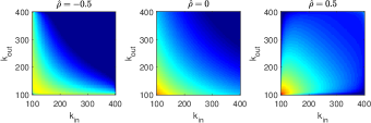
Figure 1: Log of $P(k_{in},k_{out},\hat{\rho})$ is shown for three different values of $\hat{\rho}$ (red: larger $P$, blue: smaller $P$). $a=100,b=400$.

We need to relate $\hat{\rho}$, a parameter in (29), to $\rho$, the Pearson’s correlation coefficient between in- and out-degrees of a neuron (note: not between two connected neurons). We have

$$\rho=\frac{\tilde{\Sigma}P(k_{in},k_{out},\hat{\rho})(k_{in}-\langle k\rangle)(k_{out}-\langle k\rangle)}{\sqrt{\tilde{\Sigma}P(k_{in},k_{out},\hat{\rho})(k_{in}-\langle k\rangle)^{2}}\sqrt{\tilde{\Sigma}P(k_{in},k_{out},\hat{\rho})(k_{out}-\langle k\rangle)^{2}}}$$ (30)

where $\tilde{\Sigma}$ indicates a sum over all $k_{in}$ and $k_{out}$. $\rho$ as a function of $\hat{\rho}$ is shown in Fig. 2. We see that the relationship is monotonic, and while it is possible to obtain values of $\rho$ close to 1, the lower limit is approximately $-0.6$. By varying $\hat{\rho}$ in (15) we can thus investigate the effects of varying the correlation coefficient between in- and out-degrees of a neuron ($\rho$) on the dynamics of a network. Note that for the distributions used here, treating $k$ as a continuous variable, $\langle k\rangle=2ab/(b+a)$.

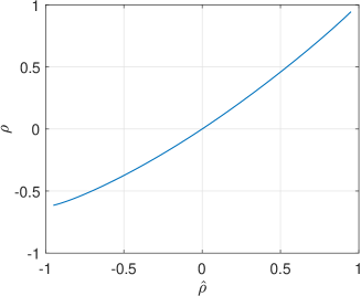
Figure 2: Correlation coefficient between in- and out-degrees, $\rho$, as a function of the correlation coefficient in the Gaussian copula, $\hat{\rho}$. Parameters: $a=100,b=400$.

Keeping in mind the normalisation $\sum_{\mathbf{k}}P(\mathbf{k})=N$ we write $Q(k_{in}^{\prime},\hat{\rho})$ as

$$Q(k_{in}^{\prime},\hat{\rho})=N\sum_{k_{out}^{\prime}=a}^{b}P(k_{in}^{\prime},k_{out}^{\prime},\hat{\rho})k_{out}^{\prime}$$ (31)

Note that the factor of $N$ here cancels with that in the last term in (15), giving equations which do not explicitly depend on $N$. Examples of $Q(k_{in}^{\prime},\hat{\rho})$ for different $\hat{\rho}$ are shown in Fig. 3. We see that increasing $\hat{\rho}$ gives more weight to high in-degree nodes and less to low in-degree nodes and vice versa.

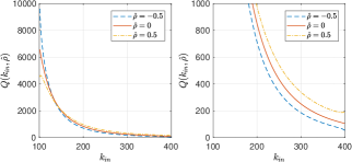
Figure 3: The function $Q(k_{in},\hat{\rho})$ (eqn. (31)) for different $\hat{\rho}$. The right panel is a zoom of the left panel. Parameters: $a=100,b=400,N=2000$.

4 Reduced model

We now turn to the issue of evaluating the sums over degrees in both (31) and (15). Although such sums are typically over only several hundred terms, it is possible to accurately evaluate them using many fewer terms, in analogy with Gaussian quadrature eng06 .

Defining an inner product as the sum

$$(f,g)=\sum_{k=a}^{b}f(k)g(k)$$ (32)

we assume that there is a corresponding set of orthogonal polynomials $\{q_{n}(k)\}_{0\leq n}$ associated with this product. These polynomials satisfy the three-term recurrence relationship

$$q_{n+1}(k)=(k-\alpha_{n})q_{n}(k)-\beta_{n}q_{n-1}(k)$$ (33)

where

$$\alpha_{n}\equiv\frac{(kq_{n},q_{n})}{(q_{n},q_{n})};\qquad 0\leq n$$ (34)

$$\beta_{n}\equiv\frac{(q_{n},q_{n})}{(q_{n-1},q_{n-1})};\qquad 1\leq n$$ (35)

$q_{0}(k)=1$ and $q_{-1}(k)=0$. Then for a given positive integer $n$, assuming that $f$ is $2n$ times continuously differentiable, we have the Gaussian summation formula

$$\sum_{k=a}^{b}f(k)=\sum_{i=1}^{n}w_{i}f(x_{i})+R_{n}$$ (36)

with error

$$R_{n}=\frac{f^{(2n)}(\xi)}{(2n)!}(q_{n},q_{n})$$ (37)

where $x_{i}$ are the $n$ roots of $q_{n}$, $\xi\in[a,b]$, and the weights $w_{i}$ are discussed below. Note that the roots of $q_{n}(k)$ are typically not integers, but this does not matter if the function $f(k)$ can be evaluated for arbitrary $k$.

In practice, to find the roots of $q_{n}$ we use the Golub-Welsch algorithm. Form the tridiagonal matrix

$$J=\begin{pmatrix}\alpha_{0}&\sqrt{\beta_{1}}&0&\dots&\dots&\dots\\ \sqrt{\beta_{1}}&\alpha_{1}&\sqrt{\beta_{2}}&0&\dots&\dots\\ 0&\sqrt{\beta_{2}}&\alpha_{2}&\sqrt{\beta_{3}}&0&\dots\\ 0&\dots&\dots&\dots&\dots&0\\ \dots&\dots&0&\sqrt{\beta_{n-2}}&\alpha_{n-2}&\sqrt{\beta_{n-1}}\\ \dots&\dots&\dots&0&\sqrt{\beta_{n-1}}&\alpha_{n-1}\end{pmatrix}$$ (38)

The eigenvalues of $J$ are the $\{x_{i}\}$ and if all eigenvectors, $v_{i}$, are scaled to have norm 1, then $w_{i}=(b-a)\left(v_{i}^{(1)}\right)^{2}$, where $v_{i}^{(1)}$ is the first component of $v_{i}$.

We will use the approximation

$$\sum_{k=a}^{b}f(k)\approx\sum_{i=1}^{n}w_{i}f(x_{i})$$ (39)

where $n\ll b-a+1$, the number of terms in the original sum. Given the resemblence of the sum on the left in (39) to the integral of $f(k)$ between $k=a$ and $k=b$, it is not surprising that the roots of $p_{n}$, when translated from the interval $[a,b]$ to $[-1,1]$, are close to the roots of the $n$th order Legendre polynomial, as would be used in Gaussian quadrature. (The same is true for the corresponding weights.)

We thus choose $n$ and write

$$Q(k_{in}^{\prime},\hat{\rho})=N\sum_{j=1}^{n}w_{j}P(k_{in}^{\prime},k_{j},\hat{\rho})k_{j}$$ (40)

where $k_{j}$ are the roots and $w_{j}$ are the weights, respectively, associated with $q_{n}(k)$. In order to use the same approximation for the sum in (15) we consider only values of $k_{in}$ equal to the $k_{j}$. As mentioned, these are typically not integers. We refer to them as “virtual degrees”. Thus our model equations are

$$\frac{\partial b(k_{j},t)}{\partial t} =\frac{-i(b(k_{j},t)-1)^{2}}{2}+\frac{(b(k_{j},t)+1)^{2}}{2}\Bigg{[}-\Delta$$

$$\left.+i\eta_{0}+\frac{iKk_{j}}{N\langle k\rangle^{2}}\sum_{j=1}^{n}w_{j}Q(k_{j},\hat{\rho})G(k_{j},t)\right]$$ (41)

for $j=1,\dots n$. We are interested in fixed points of these equations, and how these fixed points and their stabilities change as parameters such as $\eta_{0}$ and $\hat{\rho}$ are varied. We use pseudo-arclength continuation lai14B ; gov00 to investigate this.

In order to calculate the mean frequency of the network we use the result that the frequency for neurons with in-degree $k$ is monpaz15

$$f(k)=\frac{1}{\pi}\mbox{Re}\left(\frac{1-\bar{b}(k)}{1+\bar{b}(k)}\right),$$ (42)

where overline indicates complex conjugate, and then average over the network to obtain the mean frequency

$$f =\frac{\sum_{k_{in}}\sum_{k_{out}}P(k_{in},k_{out},\hat{\rho})f(k_{in})}{\sum_{k_{in}}\sum_{k_{out}}P(k_{in},k_{out},\hat{\rho})}$$

$$=\frac{\sum_{i=1}^{n}\sum_{j=1}^{n}w_{i}w_{j}P(k_{i},k_{j},\hat{\rho})f(k_{i})}{\sum_{i=1}^{n}\sum_{j=1}^{n}w_{i}w_{j}P(k_{i},k_{j},\hat{\rho})}$$ (43)

(The normalisation is needed because even though the integral of the joint degree distribution over $[k_{in},k_{out}]^{2}$ equals 1, the sum over the corresponding discrete grid does not.)

Typical convergence of a calculation of $f$ with increasing $n$ is shown in Fig. 4 for several sets of parameter values. We see rapid convergence and choose $n=15$ for future calculations. (Calculations of the form shown in Figs. 5 and 7 were repeated using the full degree sequence from $a$ to $b$, with essentially identical results.)

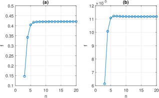
Figure 4: Mean frequency, $f$, as a function of $n$, the number of virtual degrees used. (a): $\hat{\rho}=-0.2,K=1,\eta_{0}=0.5$. (b): $\hat{\rho}=0.3,K=-0.1,\eta_{0}=-0.5$. Other parameters: $a=100,b=400,\Delta=0.05,N=2000$.

5 Results

5.1 Excitatory coupling

We first consider the case of excitatory coupling, i.e. $K>0$. We expect a region of bistability for negative $\eta_{0}$, as seen in Fig. 5. We see that decreasing $\rho$ moves the curve to the right and vice versa. ($\hat{\rho}$ was chosen to give these particular values of $\rho$.) Following the saddle-node bifurcations as $\rho$ is varied we obtain Fig. 6.

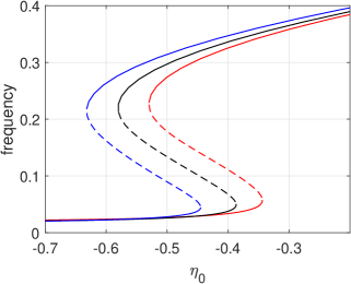
Figure 5: Mean frequency, $f$, versus $\eta_{0}$ for (left to right) $\rho=0.5,0$ and $-0.5$. Solid: stable, dashed: unstable. Parameters: $a=100,b=400,K=1.5,\Delta=0.05$.

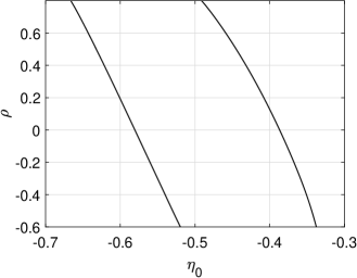
Figure 6: Continuation of the saddle-node bifurcations shown in Fig. 5. The network is bistable in the region between the curves. Parameters as in Fig. 5.

Given the influence of $\hat{\rho}$ (and thus $\rho$) on $Q$ (see Fig. 3) this result is easy to understand. Neurons with high in-degree fire faster than those with low in-degree, and for positive $\rho$, high in-degree neurons contribute more to the sum in (41) than for negative $\rho$. Thus the total amount of “output” from neurons is higher for positive $\rho$ and lower for negative $\rho$. Put another way, with positive $\rho$, neurons with high firing rate (due to high in-degree) are more likely to have a high out-degree, thus exciting more neurons than would otherwise be the case. Increasing $\rho$ has the same qualitative effect as increasing the coupling strength $K$, as observed by nykfri17 .

5.2 Inhibitory coupling

Next we consider inhibitory coupling, with $K=-1$. Average network frequency versus $\eta_{0}$ is shown in Fig. 7 for three different values of $\rho$. We see that increasing $\rho$ slightly increases the frequency and vice versa. We can also understand this behaviour in a qualitative sense. For inhibitory coupling, neurons with high in-degree are not likely to be firing, so can be ignored. When $\rho<0$, neurons with low in-degree will have high out-degree, thus the amount of inhibitory “output” in the network is increased. For positive $\rho$, neurons with low in-degree will have low out-degree, thus they will inhibit fewer neurons than in the case of negative $\rho$, leading to a higher average firing rate.

We performed calculations corresponding to the results shown in Figs. 5 and 7 for networks of theta neurons and found qualitatively, and to a large extent quantitatively, the same behaviour as in those figures (results not shown).

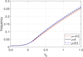
Figure 7: Mean frequency, $f$, versus $\eta_{0}$ for $\rho=-0.5,0$ and $0.5$; same colour code as in Fig. 5. All branches are stable. Parameters: $a=100,b=400,K=-1,\Delta=0.05$.

6 More realistic network

To verify the behaviour seen above in a network of theta neurons, we investigated a more realistic network of spiking neurons, in this case Morris-Lecar neurons. For the case of excitatory coupling the network equations are tsukit06

$$C\frac{dV_{i}}{dt} =g_{L}(V_{L}-V_{i})+g_{Ca}m_{\infty}(V_{i})(V_{Ca}-V_{i})$$ (44)

$$+g_{K}n_{i}(V_{K}-V_{i})$$

$$+I_{0}+I_{i}+(V_{ex}-V_{i})\frac{\epsilon}{N}\sum_{j=1}^{N}A_{ij}s_{j}$$

$$\frac{dn_{i}}{dt} =\frac{\lambda_{0}(w_{\infty}(V_{i})-n_{i})}{\tau_{n}(V_{i})}$$ (45)

$$\tau\frac{ds_{i}}{dt} =m_{\infty}(V_{i})-s_{i}$$ (46)

where

$$m_{\infty}(V) =0.5(1+\tanh{[(V-V_{1})/V_{2}]})$$ (47)

$$w_{\infty}(V) =0.5(1+\tanh{[(V-V_{3})/V_{4}]})$$ (48)

$$\tau_{n}(V) =\frac{1}{\cosh{[(V-V_{3})/(2V_{4})]}}$$ (49)

Parameters are $V_{1}=-1.2,V_{2}=18,V_{3}=12,V_{4}=17.4,\lambda_{0}=1/15msec^{-1},g_{L}=2,g_{K}=8,g_{Ca}=4,V_{L}=-60,V_{Ca}=120,V_{K}=-80,C=20\mu F/cm^{2},\tau=100,V_{ex}=120,\epsilon=5mS/cm^{2}$. Voltages are in mV, conductances are in mS/cm², time is measured in milliseconds, and currents in $\mu A/cm^{2}$. In the absence of coupling and heterogeneity a neuron undergoes a SNIC bifurcation as $I_{0}$ is increased through $\sim 40$. We have used synaptic coupling of the form in ermkop90 , but on a timescale $\tau$ rather than instantaneous as in that paper. The $I_{i}$ are randomly chosen from a Lorentzian distribution with mean zero and half-width at half-maximum $0.05$.

The network is created as follows, using the Gaussian copula of Sec. 3. For each $i\in\{1,\dots N\}$ let $x_{1}$ and $x_{2}$ be independently chosen from a unit normal distribution. Then $x_{1}$ and $y_{1}=\hat{\rho}x_{1}+\sqrt{1-\hat{\rho}^{2}}x_{2}$ both have unit normal distributions and covariance $\hat{\rho}$, i.e. are realisations of $x$ and $y$ in (17). We then set $k_{in}^{i}=C_{k}^{-1}(C(x_{1}))$ and $k_{out}^{i}=C_{k}^{-1}(C(y_{1}))$. These degrees each have distribution $p(k)$ but have correlation coefficient $\rho$, where $\rho$ is determined by the value of $\hat{\rho}$ as shown in Fig. 2. We then create the connection from neuron $j$ to neuron $i$ (i.e. set $A_{ij}=1$) with probability

$$\frac{k_{in}^{i}k_{out}^{j}}{N\langle k\rangle}$$ (50)

where $\langle k\rangle$ is the mean of the degrees, and $A_{ij}=0$ otherwise (the Chung-Lu model chulu02 ). Typical results for the network generation are shown in Fig. 8, and the measured correlations are given in the figure. The distributions of the resulting degrees no longer match the distributions of the $k_{in}^{i}$ and $k_{out}^{i}$, but are close. We could have used the configuration model to avoid this problem new03 , but here we are only interested in qualitative results. Quasi-statically sweeping through $I_{0}$ for networks with three different values of $\rho$ we obtain Fig. 9, in qualitative agreement with Fig. 5. In Fig. 5 there is a region of bistability for each value of $\rho$, and the region moves to lower average drive as $\rho$ is increased. Since we cannot detect unstable states through simulation of (44)-(46), this bistability is manifested as jumps from low frequency to high frequency branches as $I_{0}$ is varied, as seen in Fig. 9.

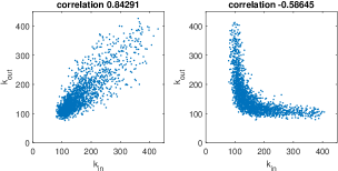
Figure 8: Degrees for a network whose generation is described in Sec. 6 for $\hat{\rho}=0.9$ (left) and $\hat{\rho}=-0.9$ (right). Parameters: $N=2000,a=100,b=400$.

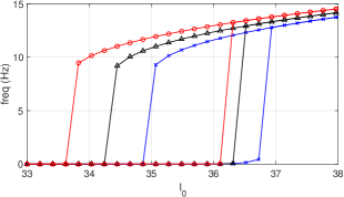
Figure 9: Mean frequency versus $I_{0}$ for a network of Morris-Lecar neurons. $N=2000$. Blue crosses: $\rho=-0.57$; black diamonds: $\rho=0$; red circles: $\rho=0.85$. $I_{0}$ is quasi-statically increased and then decreased in all cases.

For inhibitory coupling we replace $m_{\infty}(V_{i})$ in (46) by $w_{\infty}(V_{i})$, replace $V_{ex}-V_{i}$ in (44) by $V_{K}-V_{i}$, and choose $\epsilon=10mS/cm^{2}$. Sweeping through $I_{0}$ for three different values of $\rho$ we obtain Fig. 10, in qualitative agreement with Fig. 7.

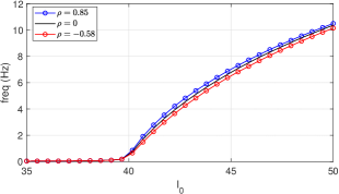
Figure 10: Mean frequency versus $I_{0}$ for networks of Morris-Lecar neurons with inhibitory coupling. $N=2000$.

7 Motifs

A number of authors have found that “motifs” (small sets of neurons connected in a specific way) do not occur in cortical networks in the proportions one would expect by chance sonsjo05 ; Perber11 . Some theoretical results relating the presence or absence of certain motifs to network dynamics have been obtained zhabev11 ; hutro13 ; ocklit15 . For networks whose generation is described in Sec. 6 we counted the number of order-2 and order-3 motifs (involving two or three neurons respectively), for negative, zero and positive values of $\rho$. We compute the frequencies (amount) of order-2 motifs by counting the amount of 0’s, 1’s and 2’s in the upper triangular part of $(A+A^{T})$, where $A$ is the adjacency matrix and $T$ means transposed. They refer to unconnected, unidirectional connected and reciprocal connected pairs of neurons, respectively. For all 13 connected order-3 motifs we used the software “acc-motif”acc-motif . The remaining three unconnected motifs have been counted by our own algorithm, i.e. looping through all neurons, we create for each a list of disconnected neurons and count among those order-2 motifs. The results are shown in Figs. 11 and 12, where counts are shown relative to the numbers found for $\rho=0$.

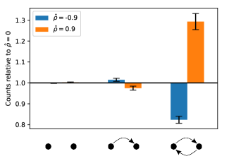
Figure 11: Relative counts of order-2 motifs. We generate three networks at a time with $\hat{\rho}\in[-0.9,0,0.9]$ to compute motif frequencies and repeat this process 100 times. Error bars indicate the standard deviation. Parameters are chosen as in Figure 8.

In all motifs with at least one reciprocal connection between two neurons, we see that the number of motifs goes up with positive $\rho$ and down with negative $\rho$. This can be understood in an intuitive way: suppose $0<\rho$ and consider a neuron with a high out-degree. It is likely to connect to a neuron with a high in-degree. But this second neuron will also have a high out-degree and is therefore more likely to connect to the first neuron, which also has a high in-degree, forming a reciprocal connection. Similarly, suppose $\rho<0$ and consider a neuron with high out-degree. It is likely to connect to a neuron with high in-degree but low out-degree. Thus it is unlikely that this second neuron will connect back to the first, which has a low in-degree.

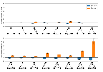
Figure 12: Relative counts of order-3 motifs.

8 Conclusion

We have investigated the effects of correlating the in- and out-degrees of spiking neurons in a structured network. We considered a large network of theta neurons, allowing us to exploit the analytical results previously derived by chahat17 , which give dynamics for complex-valued order parameters, indexed by neurons with the same degrees. The states of interest are steady states of these dynamics, and by using a Gaussian copula we were able to analytically incorporate a parameter which controls the correlations between in- and out-degrees. Numerical continuation was then used to determine the effects of varying parameters, particularly the degree correlation. In order to reduce the computational cost we introduced the concept of “virtual degrees” allowing us to efficiently approximate sums with many terms by sums with fewer terms.

For an excitatory network we found that increasing degree correlations had a similar effect as increasing the overall strength of coupling between neurons, consistent with the findings of nykfri17 ; vegrox19 . Our results are also consistent with those of vashou12 , who found that negative correlations stabilised the low firing rate state, as shown in Fig. 5. For inhibitory coupling we found that increasing degree correlations slightly increased the mean firing rate of the network. Both of these effects were reproduced in a more realistic networks of Morris-Lecar spiking neurons.

We also measured the relative frequency of occurence of order-2 and order-3 motifs as within-degree correlations were varied and found that in all motifs with at least one reciprocal connection between two neurons, the number of motifs is positively correlated with $\rho$. Several authors have linked motif statistics to synchrony within a network hutro13 ; zhabev11 , however a link between motif statistics and firing rate, as observed here, seems yet to be developed.

We chose a Lorentzian distribution of the $\eta_{i}$ in (1), as many others have done ottant08 , in order to analytically evaluate an integral and derive (6). However, we repeated the calculations shown in Figs. 5, 7, 9 and 10 using a Gaussian distribution of the $\eta_{i}$ and found the same qualitative behaviour (not shown). Regarding the parameter $n$ governing the sharpness of the function $P_{n}(\theta)$, we repeated the calculations shown in Figs. 5 and 7 for $n=5,\infty$ and obtained qualitatively the same results (not shown). We used a Gaussian copula to correlate in- and out-degrees due to its analytical form, but numerically investigated the scenarios shown in Figs. 5 and 7 for $t$ copulas and Archimedean Clayton, Frank and Gumbel copulas and found the same qualitative behaviour (also not shown).

For simplicity we used the same truncated power law distribution for both in- and out-degrees. However, the use of a Gaussian copula for inducing correlations between degrees does not require them to be the same, so one could use the framework presented here to investigate the effects of varying degree distributions rox11 , correlated or not.

We also only considered either excitatory or inhibitory networks, but it would be straightforward to generalise the techniques used here to the case of both types of neuron, with within-neuron degree correlations for either or both populations, though at the expense of increasing the number of parameters to investigate.

Conflict of interest

The authors declare that they have no conflict of interest.

References

- (1) Chandra, S., Hathcock, D., Crain, K., Antonsen, T.M., Girvan, M., Ott, E.: Modeling the network dynamics of pulse-coupled neurons. Chaos 27(3), 033102 (2017). DOI 10.1063/1.4977514
- (2) Chung, F., Lu, L.: Connected components in random graphs with given expected degree sequences. Annals of combinatorics 6(2), 125–145 (2002)
- (3) Coombes, S., Byrne, Á.: Next generation neural mass models. In: Nonlinear Dynamics in Computational Neuroscience, pp. 1–16. Springer (2019)
- (4) Eguíluz, V.M., Chialvo, D.R., Cecchi, G.A., Baliki, M., Apkarian, A.V.: Scale-free brain functional networks. Phys. Rev. Lett. 94, 018102 (2005). DOI 10.1103/PhysRevLett.94.018102. URL https://link.aps.org/doi/10.1103/PhysRevLett.94.018102
- (5) Engblom, S.: Gaussian quadratures with respect to discrete measures. Tech. rep., Uppsala University, Technical Report 2006-007 (2006)
- (6) Ermentrout, G., Kopell, N.: Oscillator death in systems of coupled neural oscillators. SIAM Journal on Applied Mathematics 50(1), 125–146 (1990)
- (7) Govaerts, W.J.: Numerical methods for bifurcations of dynamical equilibria, vol. 66. Siam (2000)
- (8) Hu, Y., Trousdale, J., Josić, K., Shea-Brown, E.: Motif statistics and spike correlations in neuronal networks. Journal of Statistical Mechanics: Theory and Experiment 2013(03), P03012 (2013)
- (9) Kähne, M., Sokolov, I., Rüdiger, S.: Population equations for degree-heterogenous neural networks. Physical Review E 96(5), 052306 (2017)
- (10) Laing, C.R.: Derivation of a neural field model from a network of theta neurons. Physical Review E 90(1), 010901 (2014)
- (11) Laing, C.R.: Numerical bifurcation theory for high-dimensional neural models. The Journal of Mathematical Neuroscience 4(1), 1 (2014)
- (12) Laing, C.R.: Bumps in small-world networks. Frontiers in Computational Neuroscience 10, 53 (2016)
- (13) LaMar, M.D., Smith, G.D.: Effect of node-degree correlation on synchronization of identical pulse-coupled oscillators. Physical Review E 81(4), 046206 (2010)
- (14) Luke, T.B., Barreto, E., So, P.: Complete classification of the macroscopic behavior of a heterogeneous network of theta neurons. Neural Computation 25, 3207–3234 (2013)
- (15) Martens, M.B., Houweling, A.R., Tiesinga, P.H.: Anti-correlations in the degree distribution increase stimulus detection performance in noisy spiking neural networks. Journal of Computational Neuroscience 42(1), 87–106 (2017)
- (16) Meira, L.A.A., Máximo, V.R., Fazenda, A.L., Da Conceição, A.F.: Acc-motif: Accelerated network motif detection. IEEE/ACM Trans. Comput. Biol. Bioinformatics 11(5), 853–862 (2014). DOI 10.1109/TCBB.2014.2321150. URL http://dx.doi.org/10.1109/TCBB.2014.2321150
- (17) Montbrió, E., Pazó, D., Roxin, A.: Macroscopic description for networks of spiking neurons. Physical Review X 5(2), 021028 (2015)
- (18) Nelsen, R.B.: An introduction to copulas. Springer Science & Business Media (2007)
- (19) Newman, M.: The structure and function of complex networks. SIAM Review 45(2), 167–256 (2003)
- (20) Nykamp, D.Q., Friedman, D., Shaker, S., Shinn, M., Vella, M., Compte, A., Roxin, A.: Mean-field equations for neuronal networks with arbitrary degree distributions. Physical Review E 95(4), 042323 (2017)
- (21) Ocker, G.K., Litwin-Kumar, A., Doiron, B.: Self-organization of microcircuits in networks of spiking neurons with plastic synapses. PLoS computational biology 11(8), e1004458 (2015)
- (22) Ott, E., Antonsen, T.: Low dimensional behavior of large systems of globally coupled oscillators. Chaos 18, 037113 (2008)
- (23) Ott, E., Antonsen, T.: Long time evolution of phase oscillator systems. Chaos 19, 023117 (2009)
- (24) Perin, R., Berger, T.K., Markram, H.: A synaptic organizing principle for cortical neuronal groups. Proceedings of the National Academy of Sciences 108(13), 5419–5424 (2011). DOI 10.1073/pnas.1016051108. URL https://www.pnas.org/content/108/13/5419
- (25) Restrepo, J.G., Ott, E.: Mean-field theory of assortative networks of phase oscillators. Europhysics Letters 107(6), 60006 (2014)
- (26) Roxin, A.: The role of degree distribution in shaping the dynamics in networks of sparsely connected spiking neurons. Frontiers in Computational Neuroscience 5, 8 (2011)
- (27) Schmeltzer, C., Kihara, A.H., Sokolov, I.M., Rüdiger, S.: Degree correlations optimize neuronal network sensitivity to sub-threshold stimuli. PloS One 10, e0121794 (2015)
- (28) Song, S., Sjöström, P.J., Reigl, M., Nelson, S., Chklovskii, D.B.: Highly nonrandom features of synaptic connectivity in local cortical circuits. PLoS biology 3(3), e68 (2005)
- (29) Tsumoto, K., Kitajima, H., Yoshinaga, T., Aihara, K., Kawakami, H.: Bifurcations in morris–lecar neuron model. Neurocomputing 69(4-6), 293–316 (2006)
- (30) Vasquez, J., Houweling, A., Tiesinga, P.: Simultaneous stability and sensitivity in model cortical networks is achieved through anti-correlations between the in- and out-degree of connectivity. Frontiers in Computational Neuroscience 7, 156 (2013)
- (31) Vegué, M., Perin, R., Roxin, A.: On the structure of cortical microcircuits inferred from small sample sizes. Journal of Neuroscience 37(35), 8498–8510 (2017). DOI 10.1523/JNEUROSCI.0984-17.2017. URL https://www.jneurosci.org/content/37/35/8498
- (32) Vegué, M., Roxin, A.: Firing rate distributions in spiking networks with heterogeneous connectivity. Phys. Rev. E 100, 022208 (2019). DOI 10.1103/PhysRevE.100.022208. URL https://link.aps.org/doi/10.1103/PhysRevE.100.022208
- (33) Zhao, L., Beverlin, B.I., Netoff, T., Nykamp, D.Q.: Synchronization from second order network connectivity statistics. Frontiers in computational neuroscience 5, 28 (2011)