Streaming Temporal Graphs: Subgraph Matching

Abstract

We investigate solutions to subgraph matching within a temporal stream of data. We present a high-level language for describing temporal subgraphs of interest, the Streaming Analytics Language (SAL). SAL programs are translated into C++ code that is run in parallel on a cluster. We call this implementation of SAL the Streaming Analytics Machine (SAM). SAL programs are succinct, requiring about 20 times fewer lines of code than using the SAM library directly, or writing an implementation using Apache Flink. To benchmark SAM we calculate finding temporal triangles within streaming netflow data. Also, we compare SAM to an implementation written for Flink. We find that SAM is able to scale to 128 nodes or 2560 cores, while Apache Flink has max throughput with 32 nodes and degrades thereafter. Apache Flink has an advantage when triangles are rare, with max aggregate throughput for Flink at 32 nodes greater than the max achievable rate of SAM. In our experiments, when triangle occurrence was faster than five per second per node, SAM performed better. Both frameworks may miss results due to latencies in network communication. SAM consistently reported an average of 93.7% of expected results while Flink decreases from 83.7% to 52.1% as we increase to the maximum size of the cluster. Overall, SAM can obtain rates of 91.8 billion netflows per day.

I Introduction

Subgraph isomorphism, the decision problem of determining for a pair of graphs, $H$ and $G$, if $G$ contains a subgraph that is isomorphic to $H$, is known to be NP-complete. Additionally, the problem of finding all matching subgraphs within a larger graph is NP-hard [17]. However, when we consider a streaming environment with bounds on the temporal extent of the subgraph, the problem becomes polynomial. We introduce some definitions to lay the groundwork for discussing complexity.

Definition 1.

Graph: $G=(V,E)$ is a graph where $V$ are vertices and $E$ are edges. Edges $e\in E$ are tuples of the form $(u,v)$ where $u,v\in V$.

Definition 2.

Temporal Graph: $G=(V,E)$ is a temporal graph where $V$ are vertices and $E$ are temporal edges. Temporal edges $e\in E$ are tuples of the form $(u,v,t,\delta)$ where $u,v\in V$ and $t,\delta\in\mathbb{R}$ and represent the start time of the edge and its duration, respectively.

Definition 3.

Streaming Temporal Graph: A graph $G$ is a streaming temporal graph when $G$ is a temporal graph where $V$ is finite and $E$ is infinite.

To express subgraph queries against a temporal graph, we need the notion of temporal contstaints on edges. First we define some notation. For an edge $e$, $starttime(e)$ returns the start time of the edge while $endtime(e)$ returns when the edge ended, i.e. $t+\delta$. We use the following simple grammar to discuss temporal constraints. It is sufficient to understand the underlying concepts and examples, but could be expanded to enable greater expressibility.

$$<Constraint> :=<EdgeExpr><Comp><EdgeExpr>|$$

$$<ArithmExpr><Comp><RealNumber>$$

$$<EdgeExpr> :=starttime(<EdgeId>)|endtime(<EdgeId>)$$

$$<ArithmExpr> :=<EdgeExpr><Op><EdgeExpr>$$

$$<Op> :=+|-$$

$$<Comp> :=<|>|<=|>=$$

Now we define Temporal Subgraph Queries using temporal constraints.

Definition 4.

Temporal Subgraph Query: For a temporal graph $G$, a temporal subgraph query is composed of a graph $H$ with edges of the form $(u,v)$, where each of the edges may have temporal constraints defined. The result of the query is all subgraphs $H^{\prime}\in G$ that are isomorphic to $H$ and that fulfill the defined temporal constraints.

Below is an example using SPARQL-like [18] syntax to express a triangular temporal subgraph query:

Listing 1: Temporal Triangle Query

⬇

{

x1 e1 x2;

x2 e2 x3;

x3 e3 x1;

starttime(e3) - starttime(e1) <= 10;

startime(e1) < starttime(e2);

starttime(e2) < starttime(e3);

}

The first part of the query with the x variables defines the subgraph structure $H$. In this example, we have defined a triangle. The second part of the query defines the temporal constraints. Edge e1 starts before e2, e2 starts before e3, and the entire subgraph must occur within a 10 second window. For temporal queries where there is a maximum window specified, and also a maximum number of edges, $d$, then the problem of finding all matching subgraphs is polynomial.

Theorem 1.

For a streaming temporal graph $G$, let $n$ be the maximum number of edges during a time duration of length $\Delta q$. A temporal subgraph query $q$ with $d$ edges and maximum temporal extent $\Delta q$ and computed on an interval of edges of length $\Delta q$ has temporal and spatial complexity of $O(n^{d})$.

Proof.

For an interval of length $\Delta q$, there are at most $n$ edges. Assume each of those $n$ edges satisfy one edge of $q$. Then there are at most $n$ potential matching subgraphs in the interval. Now assume for each of those $n$ potential matching subgraphs, each of the $n$ edges satisfies another of the edges in $q$. Then there are $n^{2}$ potential matching subgraphs. If we continue for $d$ iterations, we have a max of $n^{d}$ matching subgraphs. Thus to find and store all the matching subgraphs, it would require $O(n^{d})$ operations and $O(n^{d})$ space to store the results. ∎

The point of Theorem 1 is to show that subgraph matching on streaming data is tractable, and that over any window of time that is about the length of the temporal subgraph query, computing over that window has polynomial complexity, as long as the number of edges in the query have some maximum value. Our motivation in exploring subgraph matching on streaming data is that it fits the category of finding malicious behavior within network traffic. In our experience, cyber subgraphs of interest are generally small in size, i.e. $d<7$, and so the problem can be safely considered polynomial.

Network traffic can be thought of as streaming temporal graph where the vertices are IP addresses and the edges are communications between endpoints. For example, a watering hole attack can be thought of as subgraph pattern. In a watering hole attack, an attacker infects websites that are frequented by the targeted community. When someone from the targeted community accesses the website, their machine becomes infected and begins communicating with a machine controlled by the attacker. Figure 1 illustrates the attack.

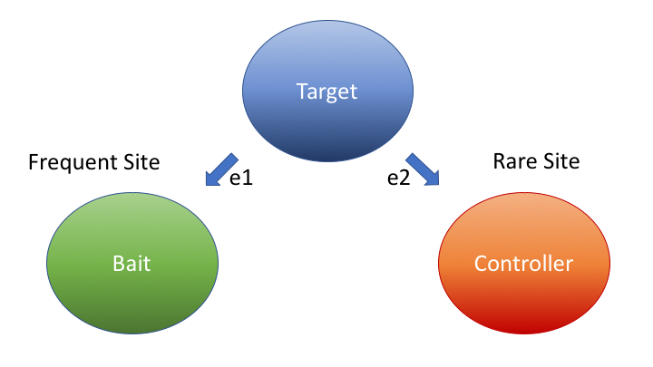
Figure 1: Illustration showing the subgraph nature of a watering hole attack. The target machine accesses a popular site, Bait. Shortly after accessing Bait, Target begins communicating to a new machine, the Controller

Listing 2 presents the watering hole query. This query has both temporal constraints on the edges and further constraints defined on the vertices, namely that bait is in Top1000, i.e. a popular site, and controller is not in Top1000, i.e. a rare or never before seen site. We use polylogarithmic streaming operators to create features for each node. However, these node-based computations are outside the scope of this paper, and presented in previous work [11].

Listing 2: Watering Hole Query

⬇

{ target e1 bait;

target e2 controller;

starttime(e2) > endtime(e1);

starttime(e2) - endtime(e1) < 20;

bait in Top1000;

controller not in Top1000; }

We benchmark two approaches for finding temporal subgraphs within a streaming graph. One approach we built from the ground up. We have a domain specific language (DSL) that we call the Streaming Analytics Language (SAL), where one can express temporal subgraph queries in a SPARQL-like[18] syntax with temporal constraints on the edges. We convert SAL into C++ using the Scala Parser Combinator [22], which allows you to express a grammar of one language which is then translated into another language. The C++ code uses a library we developed, namely the Streaming Analytics Machine (SAM). SAM is a parallel library for operating on streaming data that can run in a distributed environment.

The other approach we used builds on Apache Flink [3], which is a distributed framework purpose built for streaming applications. Flink fits many of the needs we have for streaming computations and is a good basis for comparison. While we present SAM as an implementation for SAL, nothing prevents other implementations of SAL to be developed.

To compare SAM and Flink, we focused on finding temporal triangles, i.e. the subgraph query expressed in Listing 1. Temporal triangles was chosen because they are complex enough to test the frameworks’ ability to perform difficult computations, and common enough that it could occur as a query or part of a query.

Our contributions in this work are the following:

• We present SAL as a way to quickly express queries on streaming data. In this work we focus on the subgraph matching portion of the language, which is expressed using a SPARQL-like [18] syntax. For the temporal triangle query of Listing 1, the full SAL program requires 13 lines of code while an implementation in C++ using our custom library takes 238 lines of code and an Apache Flink implementation takes 228, representing a significant savings in writing code.

• We present an implementation of SAL, using a custom built library called the Streaming Analytics Machine, or SAM. We show scaling on the temporal triangle problem to 128 nodes or 2560 cores, the maximum size of cluster we could reserve. The maximum achieved rate is 91.8 billion netflows per day.

• We compare SAM and Flink, each showing strength in a particular regime. SAM outperforms Flink when triangles are frequent.

In the next section we discuss SAL as it pertains to subgraph matching. In Section III, we discus SAM, the implementation of SAL. We then discuss the other approach using Apache Flink in Section IV, which is then followed by Section V, which compares SAM and Flink. Section VI takes a look at SAM performance when only some subgraphs match other constraints of the query besides just the subgraph portion. Section VII examines related work.Section VIII concludes.

II Streaming Analytics Language

The Streaming Analytics Language is a combination of imperative statements used for feature extraction and declarative, SPARQL-like [18] statements, used to express subgraph queries. Listing 3 gives an example program, which is a complete SAL query expressing a Watering Hole attack.

Listing 3: SAL code example

⬇

1//Preamble Statements

2WindowSize = 1000

3

4// Connection Statements

5Netflows = VastStream(”localhost”, 9999);

6

7// Partition Statements

8PARTITION Netflows By SourceIp, DestIp;

9HASH SourceIp WITH IpHashFunction;

10HASH DestIp WITH IpHashFunction;

11

12// Defining Features

13Top1000 = FOREACH Netflows

14 GENERATE topk(DestIp, 100000,

15 10000, 1000);

16

17// Subgraph definition

18Subgraph on Netflows with source(SourceIp)

19 and target(DestIp)

20{

21 target e1 bait;

22 target e2 controller;

23 starttime(e2) > endtime(e1);

24 starttime(e2) - endtime(e1) < 20;

25 bait in Top1000;

26 controller not in Top1000;

27}

In this SAL program there are five parts: 1) preamble statements, 2) partition statements, 3) connection statements, 4) feature definition, and 5) subgraph definition. Preamble statements allow for global constants to be defined that are used throughout the program. In the above listing, line 2 defines the default window size, i.e. the number of items in the sliding window.

After the preamble are the connection statements. Line 5 defines a stream of netflows called Netflows. VastStream tells the SAL interpreter to expect netflow data of a particular format (we use the same format for netflows as found in the VAST Challenge 2013: Mini-Challenge 3 dataset [25]). Each participating node in the cluster receives netflows over a socket on port 9999. The VastStream function creates a stream of tuples that represent netflows. For the tuples generated by VastStream, keywords are defined to access the individual fields of the tuple.

There are several different standard netflow formats. SAL currently supports only one format, the one used by VAST ([25]). Adding other netflow formats is a straightforward task. In fact, SAL can easily be extended to process any type of tuple. Using our current SAL interpreter, SAM, the process is to define a C++ std::tuple with the required fields and a function object that accepts a string and returns an std::tuple. Once a mapping is defined from the desired keyword (e.g. VastStream) to the std::tuple, this new tuple type can then be used in SAL connection statements. The mapping is defined via the Scala Parser Combinator [22] and is discussed in more detail in Section III.

Following the connection statements is the definition of how the tuples are partitioned across the cluster. Line 8 specifies that the netflows should be partitioned separately by SourceIp and DestIp. Each node in the cluster acts as an independent sensor and receives a separate stream of netflows. These independent streams are then re-partitioned across the cluster. In this example, each node is assigned a set of Source IP addresses and Destination IP addresses. How the IP addresses are assigned is using a common hash function. The hash function used is specified on lines 9 and 10, called the IpHashFunction. This is another avenue for extending SAL. Other hash functions can be defined and mapped to SAL constructs, similar to how other tuple types can be added to SAL. The process is to define a function object that accepts the tuple type and returns an integer, and then map the function object to a keyword using the Scala Parser Combinator.

The next part of the SAL program defines features. On line 13 we use the FOREACH GENERATE statement to calculate the most frequent destination IPs across the stream of netflows. The second parameter defines the total window size of the sliding window. The third parameter defines the size of a basic window [10], which divides up the sliding window into smaller chunks. The fourth parameter defines the number of most frequent items to keep track of.

Finally, lines 21 and 22 define the subgraph of interest in terms of declarative, SPARQL-like statements [18] that have the form $<$node$>$ $<$edge$>$ $<$node$>$. Lines 23 and 24 define temporal constraints on the edges, specifying that e1 comes before e2 and that from the end of e1 to the start of e2, the total time is twenty seconds. Lines 25 and 26 define constraints that the vertices must fulfill, in this case bait must be found in the feature set defined earlier, Top1000, while controller should not.

In this paper we focus on the subgraph queries, the specification and implementation which will be discussed in the next section.

III Streaming Analytics Machine

The Streaming Analytics Machine (SAM) is one implementation of SAL. We use the Scala Parser Combinator Library [22] to translate SAL code into C++ code which utilizes a parallel library we developed for expressing distributed streaming programs.

SAM is architected so that each node in the cluster receives tuple data Right now for the prototype, the only ingest method is a simple socket layer. In maturing SAM, other options such as Kafka [9] is an obvious alternative. We then use ZeroMQ [1] to distribute the tuples across the cluster.

For each tuple that a node receives, it performs a hash for each key specified in the PARTITION statement, and sends the tuple to the node assigned that key. For our initial domain of cyber analysis, it makes sense to partition netflows by IP address, as many types of analyses perform calculations on a per IP basis. For each netflow that a node receives, it performs a hash of the source IP in the netflow mod the cluster size to determine where to send the netflow. Similarly, for the destination IP. Thus for each netflow a node receives over the socket layer, it sends the same netflow twice over ZeroMQ. Each node is then prepared to perform calculations on a per IP basis.

For this work, we will focus on the data structures, processes, and algorithms that enable a subgraph query, such as the one in Listing 1, to be expressed in SAM and computed on a stream. First, the subgraph query is translated from the SPARQL-like syntax to a sequence of C++ objects, namely of type EdgeExpression, TimeEdgeExpression, and VertexConstraintExpression. For example, the first three lines of Listing 1 become EdgeExpressions, in essence, assigning labels to vertices and edges. The last three lines of Listing 1 become TimeEdgeExpressions, utilizing the labels specified in the EdgeExpressions to define constraints. VertexConstraintExpression’s are constraints on the vertex itself, and an example can be found in lines 25 and 26 of Listing 3. SAM uses the EdgeExpressions and TimeEdgeExpressions to develop an order of execution based upon the temporal ordering of the edges. In the example of Listing 1, $e1$ occurs before $e2$, which occurs before $e3$.

The approach we have taken assumes there is a strict temporal ordering of the edges. For our intended use case of cyber security, this is generally an acceptable assumption. Most queries have causality implicit in the question. For example, the watering hole attack is a sequence of actions, with the initial cause the malvertisement exploiting a vulnerability in a target system, which then causes other actions, all of which are temporally ordered. As another example, botnets with a command and control server, commands are issued from the command and control server, which then produces subsequent actions by the bots, which again produces a temporal ordering of the interactions. Our argument is that requiring strict temporal ordering of edges is not a huge constraint, or at the very least covers many relevant questions an analyst might ask of cyber data. We leave as future work an implementation that can address queries that do not have a temporal ordering on the edges. It should be noted that while SAM currently requires temporal ordering of edges, SAL is not so constrained. SAM can certainly be expanded to include other approaches that do not require temporal ordering of edges.

Once the subgraph query has been finalized with the order of edges determined, SAM is now set to find matching subgraphs within the stream of data. Before discussing the actual algorithm, we will first discuss the data structures.

III-A Data Structures

We make use of a number of thread-safe custom data structures, namely Compressed Sparse Row (CSR), Compressed Sparse Column (CSC), ZeroMQ Push Pull Communicator (Communicator), Subgraph Query Result Map (ResultMap), Edge Request Map (RequestMap), and Graph Store (GraphStore).

III-A1 Compressed Sparse Row

CSR is common way of representing sparse matrices. The data structure is useful for representing sparse graphs since graphs can be represented with a matrix, the rows signifying source vertices and the columns destination vertices. Instead of a $|V|\times|V|$ matrix, where $|V|$ is the number of vertices, CSR’s have space requirement $O(|E|)$, where $|E|$ is the number of edges. In the case of sparse graphs, $|E|\ll|V|\times|V|$.

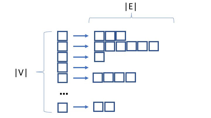
Figure 2: Traditional Compressed Sparse Row (CSR) data structure.

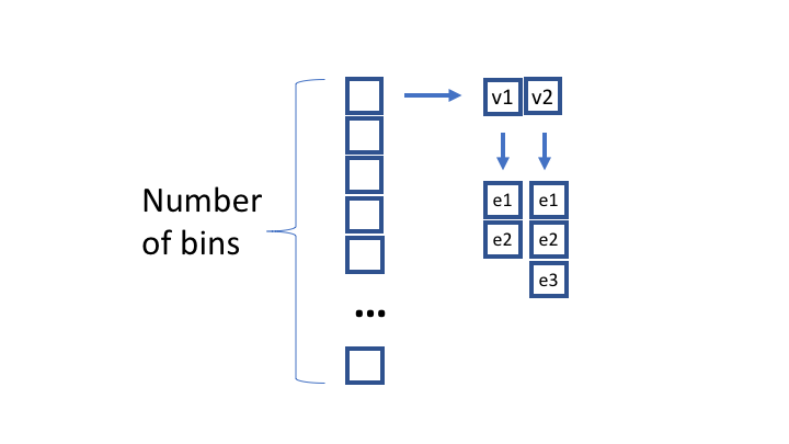
Figure 3: Modified Compressed Sparse Row (CSR) data structure.

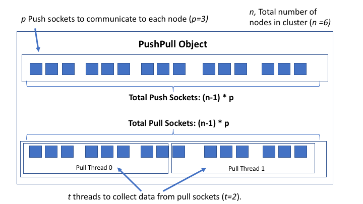
Figure 4: The push pull object.

Figure 4 presents the traditional CSR data structure. There is an array of size $|V|$ where each element of the array points to a list of edges. For array element $v$, the list of edges are all the edges that have $v$ as the source. With this index structure, we can easily find all the edges that have a particular vertex $v$ as the source. However, a complete scan of the data structure is required to find all edges that have $v$ as a destination, leading to the need for the compressed sparse column data structure, described in the next section.

CSR’s as presented work well with static data where the number of vertices and edges remain constant. However, our work requires edges that expire, and also for the possibility that vertices may come and go. To handle this situation, we create an array of lists of lists of edges, with each array element protected with a mutex. Figure 4 shows the overall structure. Instead of an array of size $|V|$, we create an array of bins that are accessed via a hash function. When an edge is consumed by SAM, it is added to this CSR data structure. The source of the edge is hashed, and if the source has never been seen, a list is added to the first level. Then the edge is added to the list. If the vertex has been seen before, the edge is added to the existing edge list. Additionally, SAM keeps track of the longest duration of a registered query, and any edges that are older than the current time minus the longest duration are deleted. Checks for old edges are done anytime a new edge is added to an existing edge list.

The CSR has mutexes protecting each bin, which will be important later when we describe finding subgraph matches. Regarding performance, as each bin has its own mutex, the chance of thread contention is very low. In metrics gathering, waiting for mutex locks of the CSR data structure has never been a significant factor in any of our experiments.

III-A2 Compressed Sparse Column

The Compressed Sparse Column (CSC) is exactly the same as the CSR, the only difference is we index on the target vertex instead of the source vertex. Both the CSR and CSC are needed, depending upon the query invoked. We may need to find an edge with a certain source (CSR), or an edge with a certain target (CSC).

III-A3 ZeroMQ PushPull Communicator

ZeroMQ handles communication between nodes using the push pull paradigm where producers push data to push sockets and consumers pull from corresponding pull sockets. The ZeroMQ PushPull Communicator (Communicator) sends messages to other nodes. There are push sockets for each node in the cluster, except for the node itself. There are corresponding pull sockets that pull the data coming from other nodes. The Communicator allows for callback functions to be registered. These callback functions are invoked whenever a pull socket receives data.

ZeroMQ opens multiple ports in the dynamic range (49152 to 65535) for each ZMQ socket that is opened logically in the code. Nevertheless, we found that contention using the ZMQ sockets created significant performance bottlenecks. As such, we created multiple push sockets per node, and anytime a node needs to send data to a node, it randomly selects one of the push sockets to use. Figure 4 gives an overview of the design. If there are $n$ nodes in the cluster and $p$ push sockets per node, in total there are $(n-1)p$ push sockets.

We also found that multiple threads were necessary to collect the data. $t$ threads are dedicated to pulling data. In our experiments, we found 4 push sockets per node and 16 total pull threads worked best for most situations.

III-A4 Subgraph Query Result Map

The ResultMap stores intermediate query results with There are two central methods, add and process. The method add takes as input an intermediate query result, creates additional query results based on the local CSR and CSC, and then creates a list of edge requests for other edges on other nodes that are needed to complete queries. The method process is similar, except in this case it takes an edge that has been received by the node and it checks to see if that edge satisfies any existing intermediate subgraph queries. The details of processing intermediate results and edges used will be discussed in greater depth in Section III-B.

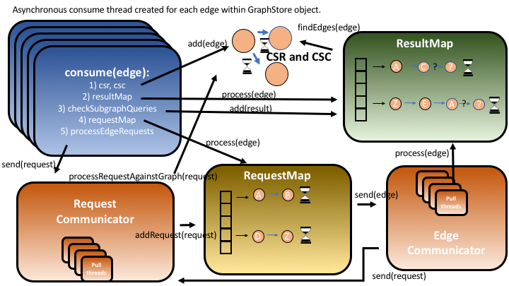
Figure 5: An overview of the algorithm employed to detect subgraphs of interest. Asynchronous threads are launched to consume each edge. The consume threads then performs five different operations. Another set of threads are pulling requests from other nodes for edges within the RequestCommunicator. Finally, one more set of threads pull edges from other nodes in reply to edge requests.

The ResultMap uses a hash structure to store results. It is an array of vectors of intermediate query results. The array is of fixed size, so must be set appropriately large to deal with the number of results generated during the max time window specified for all registered queries, otherwise excessive time is spent linearly probing the vector of intermediate results. There are mutexes protecting each access to each array slot. For each intermediate result created, it is indexed by the source, the target, or a combination of the source and target, depending on what the query needs to satisfy the next edge. The index is the result of a hash function, and that index is used to store the intermediate result within the array data structure.

III-A5 Edge Request Map

The RequestMap is the object that receives requests for edges that match certain criteria, and sends out edges to the requestors whenever an edge is found that matches the criteria. There are two important methods to mention: addRequest(EdgeRequest) and process(Edge). The addRequest method takes an EdgeRequest object and stores it. The process method takes an Edge and checks to see if there are any registered edge requests that match the given edge.

The main data structures is again a hash table. The approach to hashing is similar to the ResultMap, as it depends on whether the source is defined in the request data structure, the target is defined, or both. The index is then used to find a bin with an array of lists of EdgeRequest objects. Similar to the ResultMap, whenever process is called, edge requests that have expired are removed from the list.

III-A6 Graph Store

The GraphStore object uses all the previous data structures, orchestrating them together to perform subgraph queries. It has a pointer to the ResultMap and to the RequestMap. It also has pointers to two Communicators, one for sending/receiving edges to/from other nodes (Edge Communicator), and another for sending/receiving edge requests (Request Communicator). GraphStore maintains the CSR and CSC data structures. How all these pieces work together is described in the next section.

III-B Algorithm

The algorithm employed to find matching subgraphs employs three sets of threads: 1) GraphStore consume threads, 2) Request Communicator threads, and 3) Edge Communicator threads.

III-B1 GraphStore Consume(Edge) threads

The GraphStore object’s primary method is the consume function. GraphStore is tied into a producer, and any edges that the producer generates is fed to the consume function. For each consume call, an asynchronous thread is launched. We found that occasionally a call to consume would take an exorbitant amount of time, orders of magnitude greater than the average time. These outliers were a result of delays in the underlying ZeroMQ communication infrastructure, proving difficult to entirely prevent. As such, we added the asynchronous approach, effectively hiding these outliers by allowing work to continue even if one thread was blocked by ZeroMQ.

Each consume thread performs the following actions: 1) Adds the edge to the CSR and CSC data structures. 2) Processes the edge against the ResultMap, looking to see if any intermediate results can be further developed with the new edge. 3) Checks to see if this edge satisfies the first edge of any registered queries. If so, adds the results to the ResultMap. 4) Processes the edge against the RequestMap to see if there are any outstanding requests that match with the new edge. 5) Steps two and three can result in new edges being needed that may reside on other nodes. These edge requests are accumulated and sent out.

For steps 2-4, we provide greater detail below:

Step 2: ResultMap.process(edge): ResultMap’s process(edge) function is outlined in Algorithm 1. At the top level, the process(edge) dives down into three process(edge, indexer, checker) calls. Intermediate query results are indexed by the next edge to be matched. The srcIndexFunc, trgIndexFunc, bothCheckFunc are lambda functions that perform a hash function against the appropriate field of the edge to find where relevant intermediate results are stored within the hash table of the ResultMap. The $srcCheckFunc$ is a lambda function that takes as input a query result. It checks that the query result’s next edge has a bound source variable and an unbound target variable. Similarly, $trgCheckFunc$ returns true if the query result’s next edge has an unbound source variable and bound target variable. The $bothCheckFunc$ returns true if both variables are bound. These lambda functions are passed to the process(edge, indexer, checker) function, where the logic is the same for all three cases by using the lambda functions.

The process(edge, indexer, checker) function (line 12, uses the provided indexer to find the location (line 14) of the potentially relevant intermediate results in the hash table (class member alr). Line 15 finds the time of the edge. We use this on line 20 to judge whether an intermediate result has expired and can be deleted. On line 18 we iterate through all the intermediate results found in the bin $alr[index]$. We use the $checker$ lambda function to make sure the intermediate result is of the expected form, and if so, we try to add an edge to the result. The $addEdge$ function (line 23) adds an edge to the intermediate result if it can, and if so, returns a new intermediate result but leaves the pre-existing result unchanged. This allows the pre-existing intermediate result to match with other edges later. On line 25 we add the new result to the list, $gen$, of newly generated intermediate results. On line 31 we pass $gen$ to processAgainstGraph.

The processAgainstGraph function is used to see if there are existing edges in the CSR or CSC that can be used to further complete the queries. The overall approach is to generate frontiers of modified results, and continue processing the frontier until no new intermediate results are created. Line 39 sets the frontier to be the beginning of gen’s iterator. Then we push back a null element onto gen on line 40 to mark the end of the current frontier. Line 41 continues iterating until there are no longer any new results generated. Line 42 iterates over the frontier until a null element is reach. Lines 45 and 46 find edges from the graph that match the provided intermediate result on the frontier. Then on line 47 we try to add the edges to the intermediate result, creating new results that are added to the new frontier on line 50. Eventually the updated list of intermediate results is returned to the process(edge, indexer, checker) function. This list is then added to the hash table on line 33. The function add_nocheck is a private method that differs from the public add in that it doesn’t check the CSR and CSC, since that step has already been taken. It also generates edge requests for edges that will be found on other nodes, and that list is returned on line 35 and then in the overarching process function on line 9.

Algorithm 1 ResultMap: Processing a New Edge

1:function ResultMap.process($edge$)

2:    $requests$, a list of edge requests.

3:    $requests\mathrel{+}=process(edge,srcIndexFunc$

4:                                               $srcCheckFunc)$

5:    $requests\mathrel{+}=process(edge,trgIndexFunc,$

6:                                               $trgCheckFunc)$

7:    $requests\mathrel{+}=process(edge,bothIndexFunc,$

8:                                               $bothCheckFunc)$

9:    return $requests$

10:end function

11:

12:function ResultMap.process($edge$, $indexer$, $checker$)

13:    $gen$, a list of intermediate results generated.

14:    $index\leftarrow indexer(edge)$

15:    $currentTime\leftarrow getTime(edge)$

16:    $mutexes[index].lock()$

17:    $requests$, a list of edge requests.

18:    for all $r\in alr[index]$ do

19:       if $r.isExpired(currentTime)$ then

20:          $erase(r)$

21:       else

22:          if $checker(r)$ then

23:             $newR\leftarrow r.addEdge(edge)$

24:             if $newR$ $not$ $null$ then

25:                $gen.push\_back(newR)$

26:             end if

27:          end if

28:       end if

29:    end for

30:    $mutexes[index].unlock()$

31:    $gen\leftarrow processAgainstGraph(gen)$

32:    for all $g\in gen$ do

33:       $requests\mathrel{+}=add\_nocheck(g)$

34:    end for

35:    return $requests$

36:end function

37:

38:function ResultMap.processAgainstGraph($gen$)

39:    $frontier\leftarrow gen.begin()$

40:    $gen.push\_back(null)$

41:    while $frontier\neq gen.end()$  do

42:       while $frontier\neq null$ do

43:          if $!frontier.complete()$ then

44:             ++$frontier$

45:             $foundEdges=csr.findEdges(frontier)$

46:             $foundEdges\mathrel{+}=csc.findEdges(frontier)$

47:             for all $edge\in foundEdges$ do

48:                $newR\leftarrow frontier.addEdge(edge)$

49:                if $newR$ $not$ $null$ then

50:                   $gen.push\_back(newR)$

51:                end if

52:             end for

53:          end if

54:       end while

55:       $frontier\leftarrow frontier.erase()$

56:       $gen.push\_back(null)$

57:    end while

58:    return $gen$

59:end function

Step 3: Checking registered queries: When a GraphStore object receives a new edge, it must check to see if that edge satisfies the first edge of any registered queries. The process is outlined in Algorithm 2. The GraphStore. checkQueries(edge) function is straightforward. On line 3 we iterate through all registered queries, checking to see if the edge satisfies the first edge of the query (line 4), and if so, adds a new intermediate result to the ResultMap (line 5).

The ResultMap’s add function begins on line 11. We may create intermediate results where the next edge belongs to another node, so we initialize a list, $requests$, to store those requests (line 12). We need to check the CSR and CSC if the new result can be extended further by local knowledge of the graph. As such we make a call to processAgainstGraph on line 15. On line 16 we iterate through all generated intermediate results. If the result is not complete, we calculate an index (line 18), and place it within the array of lists of results (line 20) with mutexes to protect access. If the result is complete, we send it to the output destination (line 23). At the very end we return a list of requests, which is then aggregated by GraphStore’s checkQueries function, and then returned on line 8 and eventually used by step 5 to send out the requests to other nodes.

Algorithm 2 Checking Registered Queries

1:function GraphStore.checkQueries($edge$)

2:    $requests$, a list of edge requests.

3:    for all $q\in queries$ do

4:       if $q.satisfiedBy(edge)$ then

5:          $requests\mathrel{+}=resultMap.add(Result(edge))$

6:       end if

7:    end for

8:    return $requests$

9:end function

10:

11:function RequestMap.add($result$)

12:    $requests$, a list of edge requests.

13:    $gen$, a list of intermediate results generated.

14:    $gen.push\_back(result)$

15:    $gen\leftarrow processAgainstGraph(gen)$

16:    for all $g\in gen$ do

17:       if $!g.complete()$ then

18:          $index=g.hash()$

19:          $mutexes[index].lock()$

20:          $alr[index].push\_back(g)$

21:          $mutexes[index].unlock()$

22:       else

23:          $output(g)$

24:       end if

25:    end for

26:    return $requests$

27:end function

Step 4: RequestMap.process(edge) The purpose of RequestMap’s process(edge) is to take a new edge and find all open edge requests that match that edge. The process is detailed in Algorithm 3. The opening logic of the RequestMap.process(edge) function is similar to that of ResultMap’s process function. There are three lambda functions for indexing into RequestMap’s hash table structure, which is an array of lists of EdgeRequests ($ale$). There are also three lambda functions for checking that an edge matches a request. The indexer and the checker for each of the three cases are each passed to the process(edge, indexer, checker) function on lines 2 - 4. The process(edge, indexer, checker) function iterates through all of the edge requests with the same index as the current edge (line 11), deleteing all that have expired (line 13). If the edge matches the request, the edge is then sent to another node using the EdgeCommunicator (line 16).

Algorithm 3 RequestMap: Processing a New Edge

1:function RequestMap.process($edge$)

2:    $process(edge,srcIndexFunc,srcCheckFunc)$

3:    $process(edge,trgIndexFunc,trgCheckFunc)$

4:    $process(edge,bothIndexFunc,bothCheckFunc)$

5:end function

6:

7:function RequestMap.process($edge$, $indexer$, $checker$)

8:    $index\leftarrow indexer(edge)$

9:    $currentTime\leftarrow getTime(edge)$

10:    $mutexes[index].lock()$

11:    for all $e\in ale[index]$ do

12:       if $e.isExpired(currentTime)$ then

13:          $erase(e)$

14:       else

15:          if $checker(e,edge)$ then

16:             $edgeCommunicator.send(edge)$

17:          end if

18:       end if

19:    end for

20:    $mutexes[index].unlock()$

21:end function

III-B2 RequestCommunicator Threads

Another group of threads are the pull threads of the RequestCommunicator. These threads pull from the ZMQ pull sockets dedicated to gathering edge requests from other nodes. One callback is registered, the requestCallback. The requestCallback calls two methods: addRequest and processRequestAgainstGraph. The addRequest method registers the request with the RequestMap. The method processRequestAgainstGraph checks to see if any existing edges are already stored locally that match the edge request.

III-B3 EdgeCommunicator Threads

The last group of threads to discuss are pull threads of the EdgeCommunicator and its callback function, edgeCallback. Upon receiving an edge through the callback, ResultMap.process(edge) is called, which is discussed in detail in section III-B1. The method process(edge) produces edge requests, which are then sent via the RequestCommunicator, the same as Step 5 of GraphStore.consume(edge).

IV Apache Flink

We have currently mapped SAL into SAM as the implementation. SAL is converted into SAM code using the Scala Parser Combinator [22]. However, we wanted to compare how another framework would perform. It is certainly possible to map SAL into other languages and frameworks. A prime candidate for evaluation is Apache Flink [3], which was custom designed and built with streaming applications in mind. In this section, we outline the approach taken for implementing the triangle query of Listing 1 using Apache Flink. Once the groundwork has been laid, the actual specification of the algorithm is relatively succinct. The java code using Flink 1.6 is presented in Listing 4.

Listing 4: Apache Flink Triangle Implementation

⬇

1final StreamExecutionEnvironment env =

2 StreamExecutionEnvironment

3 .getExecutionEnvironment();

4env.setParallelism(numSources);

5env.setStreamTimeCharacteristic(

6 TimeCharacteristic.EventTime);

7

8NetflowSource netflowSource =

9 new NetflowSource(numEvents, numIps, rate);

10DataStreamSource<Netflow> netflows =

11 env.addSource(netflowSource);

12

13DataStream<Triad> triads = netflows

14 .keyBy(new DestKeySelector())

15 .intervalJoin(netflows.keyBy(

16 new SourceKeySelector()))

17 .between(Time.milliseconds(0),

18 Time.milliseconds((long) queryWindow * 1000))

19 .process(new EdgeJoiner(queryWindow));

20

21DataStream<Triangle> triangles = triads

22 .keyBy(new TriadKeySelector())

23 .intervalJoin(netflows.keyBy(

24 new LastEdgeKeySelector()))

25 .between(Time.milliseconds(0),

26 Time.milliseconds((long) queryWindow * 1000))

27 .process(new TriadJoiner(queryWindow));

28

29triangles.writeAsText(outputFile,

30 FileSystem.WriteMode.OVERWRITE);

Lines 1 - 6— define the streaming environment, such as the number of parallel sources (generally the number of nodes in the cluster) and that event time of the netflow should be used as the timestamp (as opposed to ingestion time or processing time). Lines 8 - 11 create a stream of netflows. NetflowSource is a custom class that generates the netflows in the same manner as was used for the SAL/SAM experiments. Lines 13 - 19 finds triads, which are sets of two connected edges, that fulfill the temporal requirements. The variable queryWindow on line 18 was set to be ten in our later experiments, corresponding to a temporal window of 10 seconds.

Line 15 uses an interval join. Flink has different types of joins. The one that was most appropriate for our application is the interval join. It takes elements from two streams (in this case the same stream netflows), and defines an interval of time over which the join can occur. In our case, the interval starts with the timestamp of the first edge and it ends queryWindow seconds later. This join is a self-join: it merges the netflows data stream keyed by the destination IP with the netflows data stream keyed by the source IP. In the end we have a stream of pairs of edges with three vertices of the form $A\rightarrow B\rightarrow C$.

Once we have triads that fulfill the temporal constraints, we can define the last piece: finding another edge that completes the triangle, $C\rightarrow A$. Lines 21 - 27 performs another interval join, this time between the triads and the original netflows data streams. The join is defined to occur such that the time difference between the starting time of the last edge and the starting time of the first edge must be less than queryWindow seconds.

Overall, the complete code is 228 lines long. This number includes the code that would likely need to be generated were a mapping betwen SAL and Flink completed. This includes classes to do key selection (SourceKeySelector, DestKeySelector, LastEdgeKeySelector, TriadKeySelector), the Triad and Triangle classes, and classes to perform joining (EdgeJoiner and TriadJoiner). However, the code for the Netflow class and the NetflowSource were not included, as those classes would likely be part of the library as they are with SAM. For comparison, the SAL version of this query is 13 lines long.

V Comparison: SAM vs Flink

Here we compare the performance of SAM with the custom Flink implementation. In both cases, we run the triangle query of Listing 1. We examine weak scaling, wherein the number of elements per node is kept constant as we increase the number of nodes. In all runs, each node is fed 2,500,000 netflows. For each netflow we randomly select the source and destination IPs from a pool of $|V|$ vertices for each netflow generated. We find the highest rate achievable by each approach by increasing the rate of edges production until the method to can’t keep pace.

For all of our experiments we use Cloudlab [19], a set of clusters distributed across three sites, Utah, Wisconsin, and South Carolina, where researchers can provision a set of nodes to their specifications. In particular we made use of the Wisconsin cluster using node type c220g5, which have two Intel Xeon Silver 4114 10-core CPUs at 2.20 GHz and 192 GB ECC DDR4-2666 memory per node. We vary the number of nodes to be 16, 32, 64, and 120. In Section VI we present scaling to 128 nodes for SAM, but for this batch of runs it was difficult to get a reservation for a full 128 nodes.

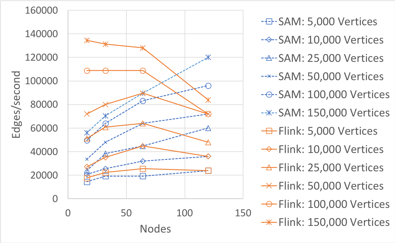
Figure 6: Shows the maximum throughput for SAM and Flink where the latency is within 15 seconds of termination.

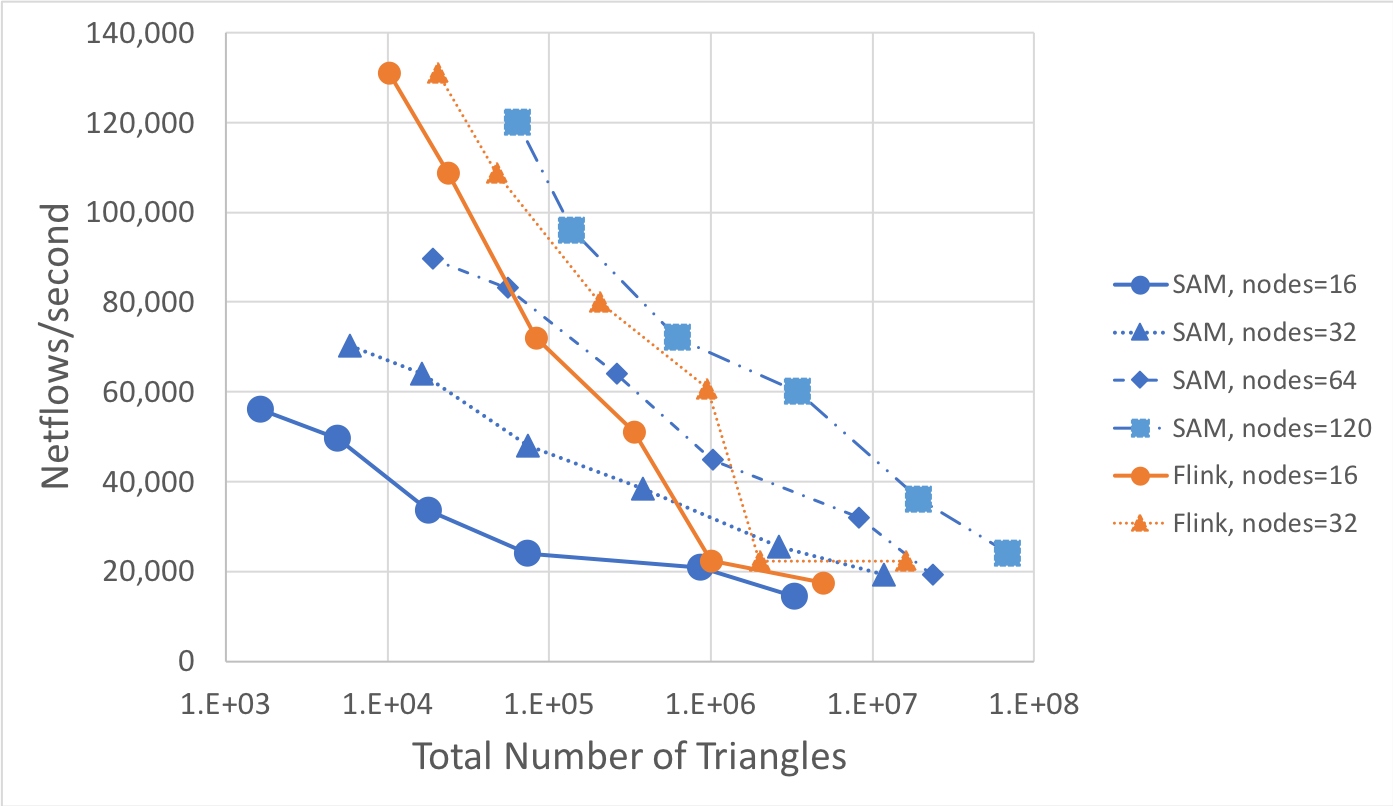
Figure 7: Presents throughput as a function of total number of triangles produced.

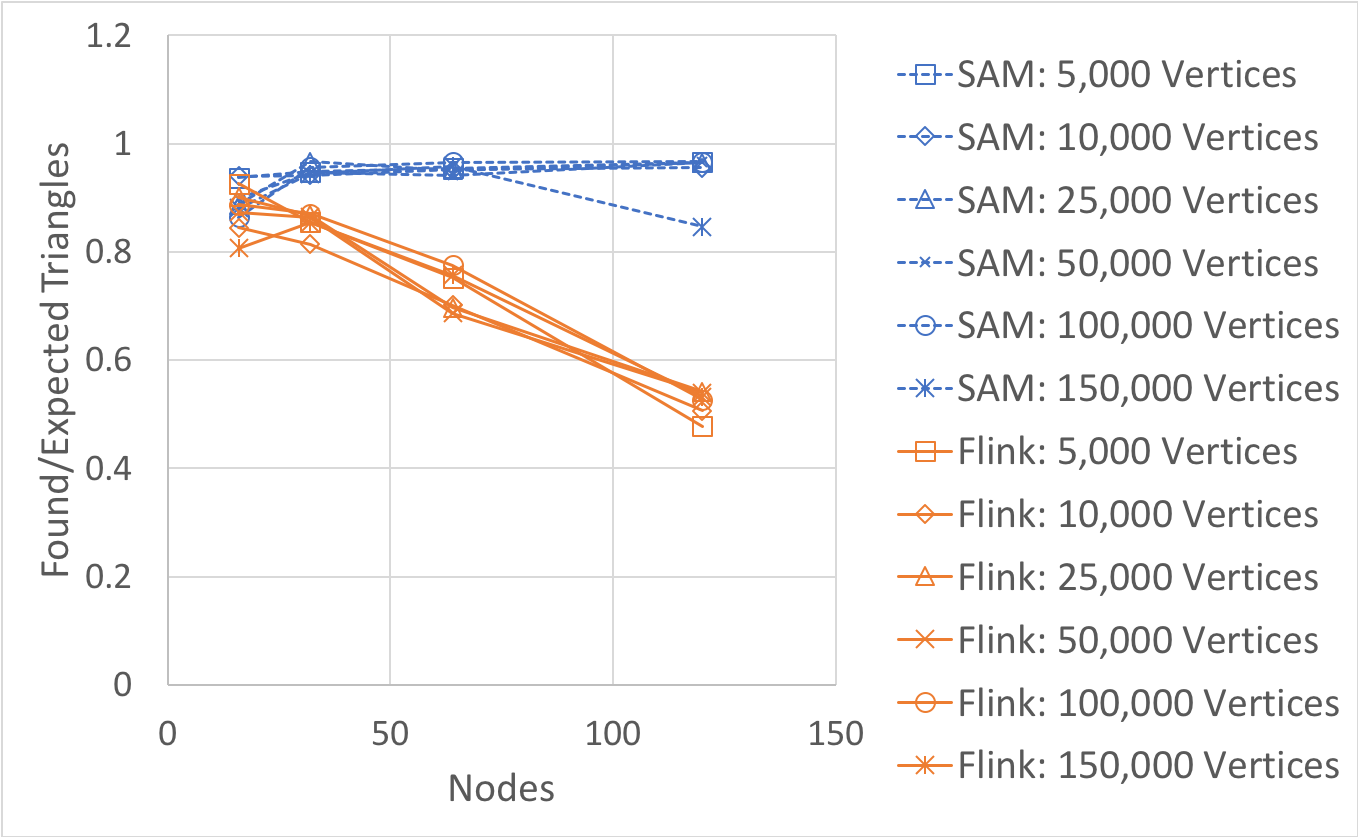
Figure 8: This graph shows the ratio of found triangles divided by the number of expected triangles.

For the Apache Flink runs we set both the job manager and task manager heap sizes to be 32 GBs. The number of taskmanager task slots was set to 1. As we only ever ran one Flink job at a time, this seemed to be the most appropriate setting. The number of sources was the size of the cluster.

For both implementations, we kept increasing throughput until run time exceeded $|V|/r+15$ seconds, where $r$ is edges produced per second. Latencies longer than 15 seconds indicated that the implementation was unable to keep pace.

Figure 8 shows the overall max aggregate throughput achieved by SAM and Flink. We varied the number of vertices, $|V|$, to be 5,000, 10,000, 25,000, 50,000, 100,000, and 150,000. Figure 8 presents the same data with another perspective, i.e. the throughput rate as a function of the total number of triangles produced. For $|V|=5,000$ or $10,000$, SAM obtained the best overall rate, continuing to garner increasing aggregate throughput to 120 nodes. Flink struggled with more than 32 nodes. While Flink continued to report results, the percentage of expected triangles fell dramatically to about 60-70% for 64 nodes, and around 50% for 120 nodes, as can be seen in Figure 8. While Flink was not able to scale past 32 nodes, it showed the best overall throughput for $|V|=50,000$ and $150,000$. $|V|=25,000$ was near the middle ground, with Flink performing slightly better, with 32 nodes obtaining an aggregate rate of 60,800 edges per second while SAM obtained 60,000 edges per second on 120 nodes.

To summarize, SAM and Flink have competing strengths. SAM scales to 120 nodes and excels when the triangle formation rate is greater than 5 per second per node. Flink does better when triangles are rare, but only scales to 32 nodes. Both show some loss due to network latencies. If some data arrives too late, it is not included in the calculations for either SAM or Flink. However, SAM has an advantages in this regard, showing consistent results throughout the processor count range which is higher than Flink.

VI Simulating other Constraints

SAL can be used not only for selecting subgraphs based on topological structure, but also on vertex constraints (e.g. see Listing 3). Here we simulate vertex constraints by randomly dropping the first edge of the triangle query, i.e. we process the netflow through SAM, but we force the edge to not match the first edge of the triangle query, giving an indication of SAM’s performance with selective queries.

We compare SAM’s performance for when we keep the first edge all of the time, 1% of the time, and .1% of the time. Figure 9 presents the results. The general trends are as expected. As we increase $|V|$, the number of triangles created decreases, and the rate goes up. Also, as we increase the rate at which edges are kept causes a decrease in the maximum achievable rate, again because more triangles are being produced, which causes a greater computational burden. The maximum achievable rate is 1,062,400 netflows per second, when we keep 0.01% of the first edges and $|V|=150,000$, or 91.8 billion per day.

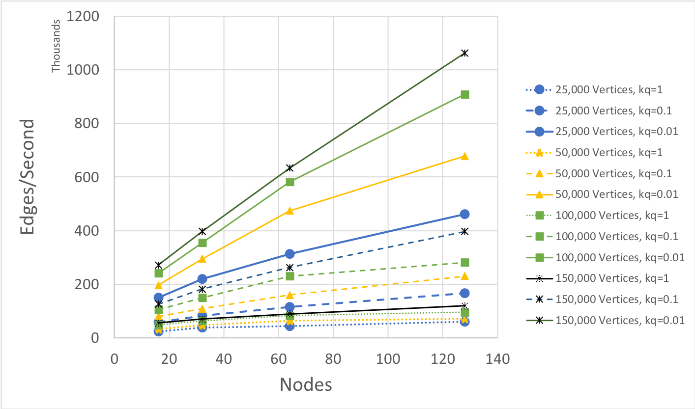
Figure 9: We keep the first edges of queries ($kq$) with probabilities $\{0.01,0.1,1\}$. We also vary $|V|$ to range from 25,000 to 150,000. This figure is a plot of edges/second versus the number of nodes.

VII Related Work

The specification of the subgraph in SAL is influenced by SPARQL [18], namely the topological structure specification. Semantic web research has produced several approaches to streaming RDF data and continuous SPARQL evaluation, namely C-SPARQL [8], Wukong [23], Wukong+S [27], EP-SPARQL [2], $SPARQL_{Stream}$ [5], and CQELS [16]. While the streaming aspect of this work is similar to our own goals, there are several aspects not addressed which our work targets, namely the temporal ordering of the edges, computing attributes on streaming data, and edges with multiple attributes. Finally, with the exception of Wukong+S [27] that report scaling numbers to 8 nodes, none of the streaming RDF/SPARQL approaches are distributed.

Recently, many frameworks have been developed that provide streaming APIs, including Storm, Spark, Flink, Heron, Samza, Beam, Gearpump, Kafka, Apex, Google Cloud Dataflow.Many could be the basis of a backend implementation for SAL. In Section V we compared Flink with SAM and found that each framework excelled in different parameter regimes. We leave as future work an exploration into combining the strengths of each approach in a unified setting.

Graph theory is an area rich with results, including a number of DSLs such as Green-Marl [13], Ligra [24], Gemini [30], Grazelle [12], and GraphIt [28]. Except for Gemini, the implementations of these DSLs target shared memory architectures. Regardless of whether these DLS approaches can be adjusted to a distributed setting, a fundamental difference between this set of work and our own is the streaming aspect of our approach and domain. An underlying assumption of these DLSs is that the data is static. The algorithmic solutions, partitioning, operation scheduling, and underlying data processing rely upon this assumption.

A plethora of efforts using vertex-centric computing exist to perform bulk synchronous parallel graph computations. Some run only on one node, [7, 29, 15] while some support distributed computations, [14, 6, 26, 4, 20]. Some support only in-memory computations [21, 6] while others can utilize out-of-core [7, 20, 29, 15]. None of the above methods provide any native support for temporal information. However, it would be possible to encode temporal information on edge data structures. The biggest impediment to using vertex-centric computing for a streaming is that it is by nature a batch process. Adapting it to a streaming environment would likely entail creating overlapping windows of time over which to perform queries in batch.

VIII Conclusions

In this paper we presented a domain specific language for expressing temporal subgraph queries on streaming data named the Streaming Analytics Language or SAL. We also presented the performance of an implementation of SAL called the Streaming Analytics Machine or SAM. We explored finding temporal triangles, and compared SAM to a custom solution written for Apache Flink. SAM excels when triangles occur frequently (greater than 5 per second per node) while Flink is best when triangles are rare. For all parameter settings, SAM showed improved throughput to 128 nodes or 2560 cores, while Flink’s rate started to decrease after 32 nodes. For more selective queries, SAM is able to obtain an aggregate rate 1 million netflows per second. While we have presented SAM as the implementation for SAL, Apache Flink shows promise as another potential underlying backend. Future work understanding the performance differences between both platforms will likely be beneficial for both approaches. We also have further evidence that programming in SAL is an efficient way to express streaming subgraph queries. SAL requires only 13 lines of code, while programming directly with SAM is 238 lines and the Flink approach is 228 lines.

References

- [1] F. Akgul. ZeroMQ. Packt Publishing, 2013.
- [2] D. Anicic, P. Fodor, S. Rudolph, and N. Stojanovic. Ep-sparql: A unified language for event processing and stream reasoning. In Proceedings of the 20th International Conference on World Wide Web, WWW ’11, pages 635–644, New York, NY, USA, 2011. ACM.
- [3] Apache. Apache flink. flink.apache.org, 2019.
- [4] Y. Bu, V. Borkar, J. Jia, M. J. Carey, and T. Condie. Pregelix: Big(ger) graph analytics on a dataflow engine. Proc. VLDB Endow., 8(2):161–172, Oct. 2014.
- [5] J.-P. Calbimonte, O. Corcho, and A. J. G. Gray. Enabling ontology-based access to streaming data sources. In Proceedings of the 9th International Semantic Web Conference on The Semantic Web - Volume Part I, ISWC’10, pages 96–111, Berlin, Heidelberg, 2010. Springer-Verlag.
- [6] R. Chen, J. Shi, Y. Chen, and H. Chen. Powerlyra: Differentiated graph computation and partitioning on skewed graphs. In Proceedings of the Tenth European Conference on Computer Systems, EuroSys ’15, pages 1:1–1:15, New York, NY, USA, 2015. ACM.
- [7] J. Cheng, Q. Liu, Z. Li, W. Fan, J. C. S. Lui, and C. He. Venus: Vertex-centric streamlined graph computation on a single pc. In 2015 IEEE 31st International Conference on Data Engineering, pages 1131–1142, April 2015.
- [8] D. Francesco Barbieri, D. Braga, S. Ceri, E. Della Valle, and M. Grossniklaus. C-sparql: A continuous query language for rdf data streams. International Journal of Semantic Computing, 4:487, 03 2010.
- [9] N. Garg. Apache Kafka. Packt Publishing, 2013.
- [10] L. Golab, D. DeHaan, E. D. Demaine, A. Lopez-Ortiz, and J. I. Munro. Identifying frequent items in sliding windows over on-line packet streams. In Proceedings of the 3rd ACM SIGCOMM Conference on Internet Measurement, IMC ’03, pages 173–178, New York, NY, USA, 2003. ACM.
- [11] E. L. Goodman and D. Grunwald. A streaming analytics language for processing cyber data. In International Conference on Machine Learning and Data Mining, 2019.
- [12] S. Grossman, H. Litz, and C. Kozyrakis. Making pull-based graph processing performant. In Proceedings of the 23rd ACM SIGPLAN Symposium on Principles and Practice of Parallel Programming, PPoPP ’18, pages 246–260, New York, NY, USA, 2018. ACM.
- [13] S. Hong, H. Chafi, E. Sedlar, and K. Olukotun. Green-marl: A dsl for easy and efficient graph analysis. In Proceedings of the Seventeenth International Conference on Architectural Support for Programming Languages and Operating Systems, ASPLOS XVII, pages 349–362, New York, NY, USA, 2012. ACM.
- [14] S. Hong, S. Salihoglu, J. Widom, and K. Olukotun. Simplifying scalable graph processing with a domain-specific language. In Proceedings of Annual IEEE/ACM International Symposium on Code Generation and Optimization, CGO ’14, pages 208:208–208:218, New York, NY, USA, 2014. ACM.
- [15] P. Kumar and H. H. Huang. G-store: High-performance graph store for trillion-edge processing. In SC ’16: Proceedings of the International Conference for High Performance Computing, Networking, Storage and Analysis, pages 830–841, Nov 2016.
- [16] D. Le-Phuoc, M. Dao-Tran, J. X. Parreira, and M. Hauswirth. A native and adaptive approach for unified processing of linked streams and linked data. In Proceedings of the 10th International Conference on The Semantic Web - Volume Part I, ISWC’11, pages 370–388, Berlin, Heidelberg, 2011. Springer-Verlag.
- [17] J. Lee, W.-S. Han, R. Kasperovics, and J.-H. Lee. An in-depth comparison of subgraph isomorphism algorithms in graph databases. In Proceedings of the 39th international conference on Very Large Data Bases, PVLDB’13, pages 133–144. VLDB Endowment, 2013.
- [18] E. Prud’hommeaux and A. Seaborne. SPARQL Query Language for RDF. W3C Recommendation, January 2008. http://www.w3.org/TR/rdf-sparql-query/.
- [19] R. Ricci, E. Eide, and The CloudLab Team. Introducing CloudLab: Scientific infrastructure for advancing cloud architectures and applications. USENIX ;login:, 39(6), Dec. 2014.
- [20] A. Roy, L. Bindschaedler, J. Malicevic, and W. Zwaenepoel. Chaos: Scale-out graph processing from secondary storage. 2015.
- [21] S. Salihoglu and J. Widom. Gps: A graph processing system. In Proceedings of the 25th International Conference on Scientific and Statistical Database Management, SSDBM, pages 22:1–22:12, New York, NY, USA, 2013. ACM.
- [22] Scala parser combinator. https://github.com/scala/scala-parser-combinators, 2017. [Online; accessed October-2017].
- [23] J. Shi, Y. Yao, R. Chen, H. Chen, and F. Li. Fast and concurrent rdf queries with rdma-based distributed graph exploration. In Proceedings of the 12th USENIX Conference on Operating Systems Design and Implementation, OSDI’16, pages 317–332, Berkeley, CA, USA, 2016. USENIX Association.
- [24] J. Shun and G. E. Blelloch. Ligra: A lightweight graph processing framework for shared memory. SIGPLAN Not., 48(8):135–146, Feb. 2013.
- [25] VAST. Vast challenge 2013: Mini-challenge 3. http://vacommunity.org/VAST+Challenge+2013 [Online; accessed October-2017].
- [26] D. Yan, Y. Huang, M. Liu, H. Chen, J. Cheng, H. Wu, and C. Zhang. Graphd: Distributed vertex-centric graph processing beyond the memory limit. IEEE Transactions on Parallel and Distributed Systems, 29(1):99–114, Jan 2018.
- [27] Y. Zhang, R. Chen, and H. Chen. Sub-millisecond stateful stream querying over fast-evolving linked data. In Proceedings of the 26th Symposium on Operating Systems Principles, SOSP ’17, pages 614–630, New York, NY, USA, 2017. ACM.
- [28] Y. Zhang, M. Yang, R. Baghdadi, S. Kamil, J. Shun, and S. P. Amarasinghe. Graphit - A high-performance DSL for graph analytics. CoRR, abs/1805.00923, 2018.
- [29] D. Zheng, D. Mhembere, R. Burns, J. Vogelstein, C. E. Priebe, and A. S. Szalay. Flashgraph: Processing billion-node graphs on an array of commodity ssds. In 13th USENIX Conference on File and Storage Technologies (FAST 15), pages 45–58, Santa Clara, CA, 2015. USENIX Association.
- [30] X. Zhu, W. Chen, W. Zheng, and X. Ma. Gemini: A computation-centric distributed graph processing system. In OSDI 16, pages 301–316, Savannah, GA, 2016. USENIX Association.