Fully-Corrective Gradient Boosting with Squared Hinge: Fast Learning Rates and Early Stopping

Abstract

Boosting is a well-known method for improving the accuracy of weak learners in machine learning. However, its theoretical generalization guarantee is missing in literature. In this paper, we propose an efficient boosting method with theoretical generalization guarantees for binary classification. Three key ingredients of the proposed boosting method are: a) the fully-corrective greedy (FCG) update in the boosting procedure, b) a differentiable squared hinge (also called truncated quadratic) function as the loss function, and c) an efficient alternating direction method of multipliers (ADMM) algorithm for the associated FCG optimization. The used squared hinge loss not only inherits the robustness of the well-known hinge loss for classification with outliers, but also brings some benefits for computational implementation and theoretical justification. Under some sparseness assumption, we derive a fast learning rate of the order ${\cal O}((m/\log m)^{-1/4})$ for the proposed boosting method, which can be further improved to ${\cal O}((m/\log m)^{-1/2})$ if certain additional noise assumption is imposed, where $m$ is the size of sample set. Both derived learning rates are the best ones among the existing generalization results of boosting-type methods for classification. Moreover, an efficient early stopping scheme is provided for the proposed method. A series of toy simulations and real data experiments are conducted to verify the developed theories and demonstrate the effectiveness of the proposed method.

I Introduction

Boosting [9] is a powerful learning scheme that combines multiple weak prediction rules to produce a strong learner with the underlying intuition that one can obtain accurate prediction by combining “rough” ones. It has been successfully used in numerous learning tasks such as regression, classification, ranking and recognition [32]. The gradient descent view of boosting [11, 12], or gradient boosting, provides a springboard to understand and improve boosting via connecting boosting with a two-step stage-wise fitting of additive models corresponding to various loss functions.

There are commonly four ingredients of gradient boosting: a set of weak learners, a loss function, an update scheme and an early stopping strategy. The weak learner issue focuses on selecting a suitable set of weak learners by regulating the property of the estimator to be found. Typical examples are decision trees [17], neural networks [2] and kernels [24]. The loss function issue devotes to choosing an appropriate loss function to enhance the learning performance. Besides the classical exponential loss in Adaboost [9], some other widely used loss functions are the logistic loss in Logit-Boosting [11], least square loss in $L_{2}$ Boosting [6] and hinge loss in HingeBoost [14]. The update scheme refers to how to iteratively derive a new estimator based on the selected weak learners. According to the gradient descent view, there are numerous iterative schemes for boosting [12]. Among these, five most commonly used iterative schemes are the original boosting iteration [9], regularized boosting iteration via shrinkage (RSBoosting) [12], regularized boosting via truncation (RTBoosting) [45], $\varepsilon$-Boosting [17] and re-scaled boosting (RBoosting) [41]. Noting that boosting is doomed to over-fit [6], the early stopping issue depicts how to terminate the learning process to avoid over-fitting. Some popular strategies to yield a stopping rule of high quality are An Information Criterion (AIC) [6], $\ell_{0}$-based complexity restriction [2] and $\ell_{1}$-based adaptive terminate rule.

The learning performance of $L_{2}$ Boosting has been rigorously verified in regression [2, 1]. In fact, under some sparseness assumption of the regression function, a learning rate of order $\mathcal{O}(m^{-1/2})$ has been provided for numerous variants of the original boosting [2, 1], where $m$ denotes the size of data set. However, for classification where $L_{2}$ Boosting performs practically not so well, there lack tight classification risk estimates for boosting as well as its variants. For example, the classification risk for AdaBoost is of an order $\mathcal{O}((\log m)^{-1})$ [4] and for some variant of Logit-Boosting is of an order $\mathcal{O}(m^{-1/8})$ [45]. There are mainly two reasons resulting in such slow learning rates. The one is that the original update scheme in boosting leads to slow numerical convergence rate [26, 28], which requires numerous boosting iterations to achieve a prescribed accuracy. The other is that the widely used loss functions such as the exponential loss and logistic loss do not admit the truncation (or clip) operator like (25) below, requiring tight uniform bounds for the derived estimator.

The aim of the present paper is to derive tight classification risk bounds for boosting-type algorithms via selecting appropriate iteration scheme and loss function. In fact, we adopt the widely used fully-corrective greedy (FCG) update scheme and the squared hinge (also called truncated quadratic) function (i.e., $\phi_{h^{2}}(t)=\max\{0,1-t\}^{2}$ for any $t\in\mathbb{R}$) as the loss function. FCG update scheme has been successfully used in [35, 33, 22], mainly in terms of the fast numerical convergence rate. Inspired by the square-type inequality [25], the squared hinge loss has been exploited to ease the computational implementation and is regarded to be an improvement of the classical hinge loss [21, 27, 23]. By taking advantage of the special form of the squared hinge loss, we develop an alternating direction method of multipliers (ADMM) algorithm [15, 13] for efficiently finding the optimal coefficients of the FCG optimization subproblem. More importantly, a tight classification risk bound is derived in the statistical learning framework [8], provided the algorithm is appropriately early stopped.

In a nutshell, our contributions can be summarized as follows.

$\bullet$ Algorithmic side: We propose a novel variant of boosting to improve its performance for binary classification. The FCG update scheme and squared hinge loss are utilized in the new variant to accelerate the numerical convergence rate and reduce the classification risk.

$\bullet$ Theoretical side: We derive fast learning rates for the proposed algorithm in binary classification. Under some regular sparseness assumption, the derived learning rate achieves an order of $\mathcal{O}((m/\log m)^{-1/4})$, which is a new record for boosting classification. If some additional noise condition is imposed, then the learning rate can be further improved to $\mathcal{O}((m/\log m)^{-1/2})$.

$\bullet$ Numerical side: We conduct a series of experiments including the toy simulations, UCI-benchmark data experiments and a real-world earthquake intensity classification experiment to show the feasibility and effectiveness of the proposed algorithm. Our numerical results show that the proposed variant of boosting is at least comparable with the state-of-the-art methods.

The rest of this paper is organized as follows. In Section II, we introduce the proposed boosting method in detail. In Section III, we provide the theoretical generalization guarantees of the proposed method. A series of toy simulations are conducted in Section IV to illustrate the feasibility of the suggested method, and some real-data experiments are provided in Section V to demonstrate the effectiveness of the proposed method. All the proofs are provided in Section VI. We conclude this paper in Section VII.

II Proposed method

In this section, after presenting the classical boosting, we introduce our variant in detail.

II-A Boosting

Boosting can be regarded as one of the most important methods in machine learning for classification and regression [31]. The original versions of boosting proposed by [30] and [9] were not adaptive and could not take full advantage of the weak learners. Latter, an adaptive boosting algorithm called AdaBoost was introduced by [10] to alleviate many practical difficulties of the earlier versions of boosting. The gradient descent view of boosting [11] then connects boosting with the well known greedy-type algorithms [38] equipped with different loss functions. In light of this perspective, numerous variants of boosting were proposed to improve its learning performance [17].

Given a data set $D=\{(x_{i},y_{i})\}_{i=1}^{m}$ with size $m$, boosting starts with a set of weak learners ${\cal G}_{n}:=\{g_{j}\}_{j=1}^{n}$ with size $n$ and a loss function $\phi$. Mathematically, it formulates the learning problem to find a function $f\in\mathrm{span}{\cal G}_{n}$ to minimize the following empirical risk

$${\cal E}_{D}^{\phi}(f):=\frac{1}{m}\sum_{i=1}^{m}\phi(y_{i},f(x_{i})),$$ (1)

where $\mathrm{span}{\cal G}_{n}$ represents the function space spanned linearly by ${\cal G}_{n}$. If $\phi$ is Fréchet differentiable, gradient boosting firstly finds a $g_{k}^{*}\in{\cal G}_{n}$ such that

$$-(\nabla{\cal E}^{\phi}_{D}(f_{k-1}),g_{k}^{*})=\sup_{g\in{\mathcal{G}}_{n}}-(\nabla{\cal E}^{\phi}_{D}(f_{k-1}),g),$$ (2)

where $(\nabla{\cal E}^{\phi}_{D}(f),h)$ denotes the value of linear functional $\nabla{\cal E}^{\phi}_{D}(f)$ at $h$. Then, it finds a $\beta_{k}^{*}\in\mathbb{R}$ such that

$${\cal E}^{\phi}_{D}(f_{k-1}+\beta_{k}^{*}g^{*}_{k})=\inf_{\beta_{k}\in\mathbb{R}}{\cal E}^{\phi}_{D}(f_{k-1}+\beta_{k}g^{*}_{k}).$$ (3)

In this way, gradient boosting yields a set of estimators $\{f_{k}\}_{k=1}^{\infty}$ iteratively and early stops the algorithm according to the bias-variance trade-off [45] to get the final estimator $f_{k^{*}}$, where $k^{*}$ is the terminal number of iterations.

According to the above description, it can be noted that the selections of weak learners, the loss function, update scheme and early stopping strategy play important roles in the practical implementation of gradient boosting. The studies in [1, 22, 12, 6, 2, 41, 45, 24] discussed the importance of the mentioned four issues respectively and then presented numerous variants of boosting accordingly.

II-B Fully-corrective greedy update scheme

There are roughly two approaches to improve the learning performance of boosting: variance-based method and bias-based method. The former focuses on controlling the structure ($\ell^{1}$ norm) of the derived boosting estimator and then reduces the variance of boosting for a fixed number of iterations, while the later devotes to accelerating the numerical convergence rates and early stopping the iteration procedure. Among these existing variants of boosting, RSBoosting [12], RTBoosting [45] and $\varepsilon$-Boosting [17] are typical variance-based methods, while RBoosting [41] is a bias-based method. The problem is, however, that the variance-based method frequently requires a large number of iterations to achieve a desired accuracy, while the bias-based method may suffer from the same problem unless some additional boundedness assumptions are imposed. An intuitive experiment is provided in Fig. 1. From Fig. 1(b), it follows that numerous iterations are required for these existing boosting methods to select a small number of weak learners.

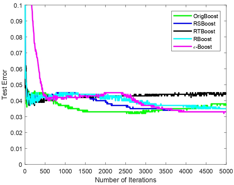
(a) Test error

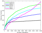
(b) Selected weak learners

Figure 1: Comparisons on boosting schemes. (a) The curves of test error for different types of boosting methods, (b) the curves of the number of selected weak learners. The detailed experimental settings can be found in Simulation IV in Sec.IV-A.

Different from above variants that can repeatedly select the same weak learners during the iterative procedure, the fully corrective greedy (FCG) update scheme proposed in [22] finds an optimal combination of all the selected weak learners. In particular, let $\{g_{j}^{*}\}_{j=1}^{k}$ be the selected weak learners at the current iteration, fully corrective greedy boosting (FCGBoosting) builds an estimator via the following minimization

$$f_{D,k}={\arg\min}_{f\in\mathrm{span}\{g_{j}^{*}\}_{j=1}^{k}}{\cal E}^{\phi}_{D}(f).$$ (4)

It should be pointed out that FCGBoosting is similar to the orthogonal greedy algorithm in approximation theory [38], fully-corrective variant of Frank-Wolfe method in optimization [20, Algorithm 4], and also orthogonal matching pursuit in signal processing [39]. The advantages of FCGBoosting lie in the sparseness of the derived estimator and the fast numerical convergence rates without any compactness assumption [33].

II-C Squared hinge loss

Since the gradient descent viewpoint connects the gradient boosting with various loss functions, numerous loss functions have been employed in boosting to enhance the performance. Among these, the exponential loss in AdaBoost, logistic loss in LogitBoost and square loss in $L_{2}$ Boosting are the most popular ones. In the classification settings, the consistency of AdaBoost and LogitBoost has been proved in [45, 4] with relatively slow learning rates. In this paper, we equip boosting with the squared hinge to improve the learning performance, both in theory and experiments.

As shown in [25], the squared hinge is of quadratic type, and thus theoretically behaves similar to the square loss and commonly better than the other typical loss functions including the exponential loss, logistic loss and hinge loss. Furthermore, learning with the squared hinge loss usually permits the margin principle [23] and thus practically performs better than the square loss for classification. Selecting the loss function $\phi$ as the squared hinge loss, i.e., $\phi_{h^{2}}(t)=(\max\{0,1-t\})^{2}$ in FCGBoosting, we can obtain a new variant of boosting summarized in Algorithm 1.

Algorithm 1 FCGBoosting with squared hinge loss

   Input: training sample set $D:=\{x_{i},y_{i}\}_{i=1}^{m}$, and a dictionary set ${\cal G}_{n}:=\{g_{j}\}_{j=1}^{n}$.

  Initialization:$f_{D,0}=0,{\cal T}^{0}=\emptyset$.

   for $k=1,2,\ldots,$

     let $g_{j_{k}}=\arg\max_{g_{j}\in{\cal G}_{n}}\ -(\nabla{\cal E}^{\phi_{h^{2}}}_{D}(f_{k-1}),g_{j})$,

     let ${\cal T}^{k}={\cal T}^{k-1}\cup\{j_{k}\}$, and

$$\text{(FCG)}\ \ f_{D,k}={\arg\min}_{f\in\mathrm{span}\{g_{j}\}_{j\in{\cal T}^{k}}}{\cal E}^{\phi_{h^{2}}}_{D}(f).$$ (5)

End until the stopping criterion is satisfied.

Notice that the FCG step (5) in Algorithm 1 is a smooth convex optimization problem, a natural algorithmic candidate is the gradient descent (GD) method. However, as shown in Fig. 2, GD needs many iterations to guarantee the convergence, which might be not efficient for the proposed boosting method, since the problem (5) in the FCG step should be solved at each iteration and there are usually numerous iterations for the proposed boosting method. Instead, we use the alternating direction method of multipliers (ADMM) due to its high efficiency and fast convergence in practice [13, 15, 19] (also, shown by Fig. 2). The convergence of the suggested ADMM algorithm (presented in Algorithm 2 in Appendix A) and its $\mathcal{O}(1/t)$ rate of convergence have been established in the existing literature (say, [13, 15, 19]).

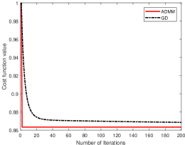
Figure 2: Comparison on the efficiency of ADMM and GD for problem (5). The samples were generated according to Section IV-A with 30% uniform random noise with $m=1000.$ The matrix $A$ was formed by the Gaussian kernel dictionary with width 0.1 and dictionary size 15. The computational time of ADMM is 0.034 seconds, while that of GD is 0.53 seconds. It can be observed that ADMM generally converges faster and more efficiently with a lower cost function value in the concerned optimization problem (5).

III Generalization Error Analysis

In learning theory [8, 37], the sample set $D=\{(x_{i},y_{i})\}_{i=1}^{m}$ with $x_{i}\in X$ and $y_{i}\in Y=\{-1,1\}$ are drawn independently according to an unknown distribution $\rho$ on $Z:=X\times Y$. Binary classification algorithms produce a classifier $\mathcal{C}:X\rightarrow Y$, whose generalization ability is measured by the misclassification error

$$\mathcal{R}(\mathcal{C})=\mathbb{P}[\mathcal{C}(x)\neq y]=\int_{X}\mathbb{P}[y\neq\mathcal{C}(x)|x]d\rho_{X},$$

where $\rho_{X}$ is the marginal distribution of $\rho$ and $\mathbb{P}[y|x]$ is the conditional probability at $x\in X$. The Bayes rule $f_{c}(x)=\mathrm{sgn}(\eta(x)-1/2)$ minimizes the misclassification error, where $\eta(x)=\mathbb{P}[y=1|x]$ is the Bayes decision function and $\mathrm{sgn}(t)=1$ if $t\geq 0$ and otherwise, $\mathrm{sgn}(t)=-1$. Since $f_{c}$ is independent of the classifier $\mathcal{C}$, the performance of $\mathcal{C}$ can be measured by the excess misclassification error $\mathcal{R}(\mathcal{C})-\mathcal{R}(f_{c})$. For the derived estimator $f_{D,k}$ in Algorithm 1, we have $\mathcal{C}=\mathrm{sgn}(f_{D,k}(x))$. Then, it is sufficient to present a bound for $f_{D,k}(x)-(\eta(x)-1/2)$. With this, we at first present a sparseness assumption on $\eta(x)-1/2$.

Assumption 1.

There exists an $h_{0}\in\mathrm{span}{\cal G}_{n}$ such that

$$\|\eta-1/2-h_{0}\|_{\rho}\leq C_{1}n^{-r},\ \text{and}\ \|h_{0}\|_{\ell^{1}}\leq C_{2},$$ (6)

for some positive constants $r,C_{1},C_{2}$.

Assumption 1 requires that $\eta(x)-1/2$ should be sparsely approximated by the set of weak learners with certain fast decay of some polynomial order. Such an assumption is regular in the analysis of boosting algorithm and has been adopted in large literature [45, 4, 2, 38, 26, 1, 33, 24, 28, 41]. Under this assumption, we can derive the following learning rate for FCGBoosting

Theorem 1.

Let ${\cal G}_{n}:=\{g_{j}\}_{j=1}^{n}$ be a set of weak learners with $\|g_{j}\|_{\infty}\leq 1$, $j=1,\dots,n$. Under Assumption 1, if $n\sim m^{a}$ for $a\geq 1$, $r\geq\frac{1}{4a}$ and $k\sim\sqrt{\frac{m}{\log m}}$, then for any $0<\delta<1$, with confidence at least $1-\delta$, there holds

$${\cal R}(\mathrm{sgn}(f_{D,k}))-{\cal R}(f_{c})\leq C_{3}\left(\frac{m}{\log m}\right)^{-1/4}\log\frac{4}{\delta},$$

where $C_{3}$ is a positive constant independent of $\delta$ or $m$.

The proof of this theorem will be presented in Section VI. This theorem provides some early stopping of the proposed version of boosting method under the assumption that the Bayes decision function can be well approximated by combining weak learners. From Theorem 1, an optimal $k$ should be set as in the order of ${\cal O}(\sqrt{\frac{m}{\log m}})$, which shows that the number of selected weak learners is significantly less than $m$ and $n$. It should be noted that the derived learning rate in Theorem 1 is of the same order of FCGBoosting with the square loss [2] under the same setting. To further improve the learning rate, the following Tsybakov noise condition [40] is generally required.

Assumption 2.

Let $0\leq q\leq\infty.$ There exists a positive constant $\hat{c}_{q}$ such that

$$\rho_{X}(\{x\in X:|\eta(x)-1/2|\leq\hat{c}_{q}t\})\leq t^{q},\quad\forall t>0.$$

The Tsybakov noise assumption measures the size of the set of points that are corrupted with high noise in the labeling process, and always holds for $q=0$ with $\hat{c}_{q}=1$. It is a standard noise assumption in classification which has been adopted in [36, 43, 25, 44] to derive fast learning rates for classification algorithms. Under the Tsybakov noise assumption, we can improve the rate as follows.

Theorem 2.

Let ${\cal G}_{n}:=\{g_{j}\}_{j=1}^{n}$ be a set of weak learners with $\|g_{j}\|_{\infty}\leq 1$, $j=1,\dots,n$. Under Assumption 1 and Assumption 2 with $0\leq q<\infty$, if $n\sim m^{a}$ for $a\geq 1$, $r\geq\frac{1}{4a}$ and $k\sim\sqrt{\frac{m}{\log m}}$. Then for any $0<\delta<1$, with confidence at least $1-\delta$, there holds

$${\cal R}(\mathrm{sgn}(f_{D,k}))-{\cal R}(f_{c})\leq C_{4}\left(\frac{m}{\log m}\right)^{-\frac{q+1}{2(q+2)}}\log\frac{4}{\delta},$$

where $C_{4}$ is a positive constant independent of $\delta$ or $m$.

The proof of this theorem is also postponed to Section VI. Note that when $q=0$, the learning rate established in Theorem 2 reduces to that of Theorem 1, while when $q=\infty$, the obtained learning rate in Theorem 2 approaches to $\left(\frac{m}{\log m}\right)^{-1/2}$, which is a new record for the boosting-type methods under the classification setting.

IV Toy Simulations

In this section, we present a series of toy simulations to demonstrate the feasibility and effectiveness of FCGBoosting. All the numerical experiments were carried out in Matlab R2015b environment running Windows 8, Intel(R) Xeon(R) CPU E5-2667 v3 @ 3.2GHz 3.2GH.

IV-A Experimental settings

The settings of simulations are similar to that in [44] described as follows.

Samples: In simulations, the training samples were generated as follows. Let

$$\zeta(t)=\left((1-2t)_{+}^{5}(32t^{2}+10t+1)+1\right)/2,\qquad t\in[0,1]$$

be a nonlinear Bayes rule. Let ${\bf x}=\{x_{i}\}_{i=1}^{m}\subset([0,1]\times[0,1])^{m}$ be drawn i.i.d. according to the uniform distribution with size $m$. Then we labeled the samples lying in the epigraph of function $\zeta(t)$ as the positive class, while the rest were labeled as the negative class, that is, given an $x_{i}=(x_{i}(1),x_{i}(2))$, its label $y_{i}=1$ if $x_{i}(2)\geq\zeta(x_{i}(1))$, and otherwise, $y_{i}=-1.$ Besides the uniformly random noise generally considered in regression, we mainly focused on the outlier noise in our simulations, that is, the noisy samples lying in the region that is far from the Bayes (see, Fig. 3). We considered different widths (i.e., tol) and noise ratios (i.e., ratio) with the banded region.

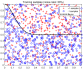
(a) uniform random noise

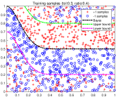
(b) outlier noise

Figure 3: The generated training samples with uniform random noise (see, figure (a)) and outlier noise (see, figure (b)) used in simulations. The red points are labeled as “+1” class, while the blue points are labeled as “-1” class. In the title of figure (b), the notation tol=0.3 represents that the difference between the Bayes rule and upper (lower) bound is 0.3, while the notation ratio=0.4 represents that the noise ratios in both left-lower and right-upper regions are 0.4. The total noise level in this case is 17.4%.

Implementation and Evaluation: We implemented four simulations to illustrate the effect of parameters and show the effectiveness of the proposed version of boosting method. For each simulation, we repeated $20$ times of experiments and recorded the test error, which is defined as the ratio of the number of misclassified test labels to the test sample size. The first one is to illustrate the effect of the number of iterations $k$, which is generally exploited for setting the stopping rule of the proposed method. The second one is to demonstrate the effect of the number of dictionaries $n$. The third one is to show the feasibility and effectiveness of the used squared hinge loss (i.e., $\phi_{h^{2}}(x)=(1-x)_{+}^{2}$) via comparing with some other loss functions including the square loss with $\phi_{sq}(x)=(1-x)^{2}$, the hinge loss with $\phi_{h}(x)=(1-x)_{+}$ and the cubed hinge loss with $\phi_{h^{3}}(x)=(1-x)_{+}^{3}$ [21]. The final one is to show the outperformance of the fully-corrective update scheme via comparing to the existing popular update scheme used in gradient boosting. Since the performance of boosting-type methods also depends on the dictionary type, in this paper, we considered four types of dictionaries, that is, the dictionaries formed by the Gaussian kernel, polynomial kernel, and the neural network kernels with sigmoid and rectified linear unit (ReLU) activations, respectively, and henceforth, they are respectively called Gauss, polynomial, sigmoid, Relu for short. We set empirically the parameters of ADMM algorithm (i.e., Algorithm 2) used in the FCG optimization step as follows: $\alpha=1$, $\gamma=1$ and the maximal number of iterations was set as 100.

IV-B Simulation Results

In this part, we report the experimental results and present some discussions.

Simulation 1: On effect of number of iterations $k$. From Algorithm 1, the number of iterations $k$ is a very important algorithmic parameter, which is generally set as the stopping rule of the boosting type of methods. By Theorems 1 and 2, a moderately large $k$ (i.e., $k\sim\sqrt{\frac{m}{\log m}}$) is required to achieve the optimal generalization performance. To illustrate the effect of the number of iterations $k$, we randomly generated training and test samples with both sizes being $m=1000$. We considered both noise types in training samples, i.e., uniformly random noise with the noise level 30%, and the outlier noise with $tol=0.3$ and $ratio=0.4$ (in this case, the level of outlier noise is 17.4%), as described in Section IV-A . Moreover, we considered four different dictionaries formed by Gaussian kernel, polynomial kernel, neural network kernel with sigmoid and neural network kernel with ReLU activation, respectively, where the sizes of all four dictionaries are the same $n=1000$. We varied $k$ according to the set of size 11, i.e., $\left\{\left\lceil\frac{1}{2}\sqrt{\frac{m}{\log m}}\right\rceil,\left\lceil\sqrt{\frac{m}{\log m}}\right\rceil,2\left\lceil\sqrt{\frac{m}{\log m}}\right\rceil,\ldots,10\left\lceil\sqrt{\frac{m}{\log m}}\right\rceil\right\}$, and recorded the associated test error. In this experiment, $\left\lceil\sqrt{\frac{m}{\log m}}\right\rceil=13$ since $m=1000$. The curves of test error are shown in Fig. 4.

From Fig. 4, the trends of test error for different dictionaries are generally similar, that is, as $k$ increasing from $\left\lceil\frac{1}{2}\sqrt{\frac{m}{\log m}}\right\rceil$ to $10\left\lceil\sqrt{\frac{m}{\log m}}\right\rceil$, the test error generally decreases firstly and then becomes stable. This phenomenon is mainly due to that when $k$ is small, the selected model might be under-fitting, and then increasing $k$ shall improve the generalization ability. More specifically, in both uniform and outlier noise cases, it is generally sufficient to set the iteration number $k$ as $5\left\lceil\sqrt{\frac{m}{\log m}}\right\rceil$ by Fig. 4. This in some extent verifies our main theorems (i.e., Theorems 1 and 2), which show that the moderately large $k$ is in the order of $\left\lceil\sqrt{\frac{m}{\log m}}\right\rceil$. Motivated by this experiment, in practice, the maximal number of iterations $k$ for the proposed boosting method can be empirically chosen from these five values $\left\{\left\lceil\sqrt{\frac{m}{\log m}}\right\rceil,2\left\lceil\sqrt{\frac{m}{\log m}}\right\rceil,\ldots,5\left\lceil\sqrt{\frac{m}{\log m}}\right\rceil\right\}$ via cross validation. When comparing with these differen dictionaries, the generalization performance of Relu are slightly better than the other three dictionaries in both noise cases.

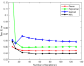
(a) 30% Uniform random noise

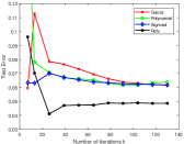
(b) 17.4% Outlier noise

Figure 4: Effect of the number of iterations $k$. (a) the curves of test error of four different dictionaries with respect to $k$ under the 30% uniform random noise, (b) the curves of test error under the 17.4% outlier noise where $tol=0.3$ and $ratio=0.4$.

Simulation 2: On effect of size of dictionary set $n$. Given a dictionary type, the size of dictionary set $n$ generally reflects the approximation ability of the given dictionary set. Particularly, according to Assumption 1, one prerequisite condition for the boosting type methods is that the underlying learner should be well-approximated by the chosen dictionary set. However, a larger dictionary set usually brings more computational cost. Thus, it is meaningful to verify the possible optimal size of dictionary set. To illustrate this, in this experiment, the training and test samples were generated in the same way of Simulation 1. Instead of varying the number of iterations $k$, we varied the size of dictionary set $n$ from $m$ to $10m$, where $m=1000$ is the size of training samples. For each $n$, the number of iterations $k$ was chosen from these five values $\left\{\left\lceil\sqrt{\frac{m}{\log m}}\right\rceil,2\left\lceil\sqrt{\frac{m}{\log m}}\right\rceil,\ldots,5\left\lceil\sqrt{\frac{m}{\log m}}\right\rceil\right\}$ via cross validation. The curves of test error with respective to the number of dictionary sets $n$ are shown in Fig. 5.

From Fig. 5, the number of dictionary set $n$ has little effect on the generalization performance for all types of dictionaries and in both noise settings, when $n$ is in the order of ${\cal O}(m)$. This is also verified by our main theorems (i.e., Theorems 1 and 2). By Theorems 1 and 2, $n$ should be in the order of ${\cal O}(m^{a})$ for some $a\geq 1$ to achieve the optimal learning rates. Specifically, in this experiment, we show that the generalization performance of the proposed method does not vary very much when $n$ varies from $m$ to $m^{4/3}$. In our latter experiments, we empirically set $n=m$ in the consideration of both generalization performance and computational cost. Regarding the performance of the different dictionaries, we observed that the performance of Relu and Gauss is slightly better than that of polynomial and sigmoid.

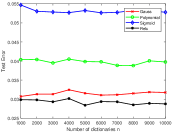
(a) 30% Uniform random noise

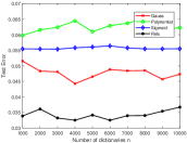
(b) 17.4% Outlier noise

Figure 5: Effect of the number of dictionaries $n$. (a) the curves of test error of four different dictionaries with respect to $n$ under the 30% uniform random noise, (b) the curves of test error under the 17.4% outlier noise where $tol=0.3$ and $ratio=0.4$.

Simulation 3: On comparison among different losses. In this experiment, we compare the performance of the fully-corrective greedy boosting method with different loss functions, including the square loss $\phi_{sq}(x)=(1-x)^{2}$, the hinge loss $\phi_{h}(x)=(1-x)_{+}$, the suggested squared hinge loss $\phi_{h^{2}}(x)=(1-x)_{+}^{2}$ and the cubed hinge loss $\phi_{h^{3}}=(1-x)_{+}^{3}$. Note that the hinge loss is non-differentiable, while both the squared hinge and cubed hinge losses are differentiable. As demonstrated in the literature [27, 23, 21], the differentiability of squared hinge loss brings many benefits to both the computational implementation and theoretical analysis. In this experiment, we are willing to show the similar benefits brought by the squared hinge loss. Specifically, the training and test samples were generated via the similar way as described in Simulation 1. Moreover, we considered different noise levels for both uniform random and outlier noise. For each case, we repeated $20$ times of experiments and record the averages of their test errors. The test errors for different losses are presented in Table I and Table II.

From Table I and Table II, the performance of the suggested squared hinge loss is commonly slightly better than the other three loss functions. When comparing the performance of different dictionaries, by Tables I and II, the performance of Gauss and Relu are frequently better than that of polynomial and sigmoid, which is also observed in the previous experiments. These show the effectiveness of the suggested squared hinge loss via comparing with the other loss functions.

TABLE I: Comparison on the test errors of different losses in different levels of uniform random noise. The best results among different losses are marked in bold.

Dictionary	20% uniform random				30% uniform random				40% uniform random
	$\phi_{h^{2}}$	$\phi_{h}$	$\phi_{h^{3}}$	$\phi_{sq}$	$\phi_{h^{2}}$	$\phi_{h}$	$\phi_{h^{3}}$	$\phi_{sq}$	$\phi_{h^{2}}$	$\phi_{h}$	$\phi_{h^{3}}$	$\phi_{sq}$
Gauss	0.0239	0.0265	0.0295	0.0283	0.0418	0.0419	0.0419	0.0431	0.0851	0.0879	0.0882	0.0891
Polynomial	0.0248	0.0265	0.0276	0.0289	0.0425	0.0403	0.0436	0.0490	0.0879	0.0929	0.0935	0.0929
Sigmoid	0.0524	0.0693	0.0479	0.0271	0.0597	0.0768	0.0589	0.0433	0.0922	0.0925	0.0895	0.0963
Relu	0.0219	0.0394	0.0266	0.0288	0.0335	0.0503	0.0397	0.0453	0.0810	0.0864	0.0850	0.1

TABLE II: Comparison on the test errors of different losses in different levels of outlier noise with the same $tol=0.3$ and different $ratios$ varying from $0.2$ to $0.4$, where the associated noise levels are 8.51%, 12.83% and 17.31%, respectively. The best results among different losses are marked in bold.

Dictionary	8.51% outlier noise				12.83% outlier noise				17.31% outlier noise
	$\phi_{h^{2}}$	$\phi_{h}$	$\phi_{h^{3}}$	$\phi_{sq}$	$\phi_{h^{2}}$	$\phi_{h}$	$\phi_{h^{3}}$	$\phi_{sq}$	$\phi_{h^{2}}$	$\phi_{h}$	$\phi_{h^{3}}$	$\phi_{sq}$
Gauss	0.0125	0.0136	0.0126	0.0145	0.0171	0.0195	0.0255	0.0237	0.0450	0.0548	0.0498	0.0714
Polynomial	0.0157	0.0184	0.0170	0.0172	0.0245	0.0238	0.0327	0.0332	0.0608	0.0550	0.0737	0.0866
Sigmoid	0.0554	0.0584	0.0514	0.0152	0.0512	0.0634	0.0487	0.0317	0.0629	0.0701	0.0657	0.0770
Relu	0.0129	0.0134	0.0149	0.0141	0.0156	0.0212	0.0211	0.0272	0.0380	0.0385	0.0405	0.0745

Simulation 4: On comparison among different update schemes. In this experiment, we provided some comparisons between fully-corrective update and most of the existing types of update schemes such as that in the original boosting scheme (called OrigBoosting for short) in [10], the regularized boosting with shrinkage (called RSBoosting for short) in [12], the regularized boosting with truncation (called RTBoosting) in [45], the forward stagewise boosting (called $\epsilon$-Boosting for short) in [18], and the rescaled boosting (called RBoosting for short) suggested in the recent paper [41], when adopted to the empirical risk minimization with the squared hinge loss over the Gaussian type dictionary. The optimal width of the Gaussian kernel was determined via cross validation from the set $\{0.1,0.5,1,5\}$. Specifically, the training and test samples were generated according to Section IV-A, where the numbers of training and test samples were both $1,000$ and the training samples were generated with 30% uniform random noise. The size of the total dictionaries generated was set as $10000$. The maximal number of iterations for the proposed FCGBoosting was set as 500, while for the other types of boosting methods, the maximal number of iterations was set as $5000$. For each trail, we recorded the optimal test error with respect to the number of iterations, and the associated training error as well as number of dictionaries selected. The averages of the optimal test error, training error and number of dictionaries selected over 10 repetitions are presented in Table III.

As shown in Table III, the performance of all boosting methods with the optimal number of dictionaries are almost the same in terms of the generalization ability measured by the test error, and under these optimal scenarios, all the boosting methods are generally well-fitted in the perspective of training error. As demonstrated by Table III and Fig. 1(a), the most significant advantage of the adopted fully-corrective update scheme o is that the number of dictionaries for FCGBoosting is generally far less than that of the existing methods such as OrigBoosting, RSBoosting, RTBoosting, $\epsilon$-Boosting and RBoosting. Particularly, from Table III, the average number of dictionaries for the proposed FCGBoosting is only $12.6$, which is very close to the theoretical value $\left\lceil\sqrt{\frac{m}{\log m}}\right\rceil=13$ as suggested in Theorem 1, where in this experiment $m=1000$. Moreover, from Fig. 1(b), most of the partially-corrective greedy type boosting methods select new dictionaries slowly after certain iterations, while their generalization performance improves also very slowly.

TABLE III: Comparisons among different types of boosting methods.

Boosting type	OrigBoosting [10]	RSBoosting [12]	RTBoosting [45]	$\epsilon$-Boosting [18]	RBoosting [41]	FCGBoosting (this paper)
Test error	0.0238	0.0256	0.0239	0.0256	0.0221	0.0229
Training error	0.3071	0.3074	0.3069	0.3077	0.3078	0.3076
Dictionary no.	103.8	140.1	72.2	313.1	120.8	12.6

V Real data experiments

In this section, we show the effectiveness of the proposed method via a series of experiments on 11 UCI data sets covering various areas, and an earthquake intensity classification dataset.

V-A UCI Datasets

Samples. All data is from: https://archive.ics.uci.edu/ml/ datasets.html. The sizes of data sets are listed in Table IV. For each data set, we used $50\%$, $25\%$ and $25\%$ samples as the training, validation and test sets, respectively.

Competitors. We evaluated the effectiveness of the proposed boosting method via comparing with the baselines and five state-of-the-art methods including two typical support vector machine (SVM) methods with radial basis function (SVM-RBF) and polynomial (SVM-Poly) kernels respectively, and a fast polynomial kernel based method for classification recently proposed in [44] called FPC, and the random forest (RF) [5] and AdaBoost [10]. We used the well-known libsvm toolbox to implement these SVM methods, from the website: https://www.csie.ntu.edu.tw/ cjlin/libsvm/. For the proposed method, we also considered four dictionaries including Gauss, Polynomial, Sigmoid and Relu.

Implementation. For the proposed boosting method, we set $\alpha=1$, $\gamma=1$, the initialization $(u^{0},v^{0},w^{0})=(0,y,0)$ and the maximal number of iterations $T=100$ for the ADMM method used in the FCG step; the stopping criterion of the suggested method was set as the maximal iterations less than $K$, where $K$ was chosen from these five values $\left\{\left\lceil\sqrt{\frac{m}{\log m}}\right\rceil,2\left\lceil\sqrt{\frac{m}{\log m}}\right\rceil,\ldots,5\left\lceil\sqrt{\frac{m}{\log m}}\right\rceil\right\}$ via cross validation; the size of the dictionary set was set as the number of training samples $m$. These empirical settings are generally adequate as shown in the previous simulations.

For both SVM-RBF and SVM-Poly, the ranges of parameters $(c,g)$ involved in libsvm were determined via a grid search on the region $[2^{-5},2^{5}]\times[2^{-5},2^{5}]$ in the logarithmic scale, while for SVM-Poly, the kernel parameter was selected from the interval [1, 10] via a grid search with 10 candidates, i.e., $\{1,2,\ldots,10\}$. The kernel parameter of FPC was selected similarly to SVM-Poly.

For RF, the number of trees used was determined from the interval $[2,20]$ via a grid search with 10 candidates, i.e., $\{2,4,\ldots,20\}$. For AdaBoost, the number of trees used was set as 100. For each data set, we ran $50$ times of experiments for all algorithms, and then record their averages of test accuracies, which is defined as the percentage of the correct classified labels.

TABLE IV: Sizes of UCI data sets. In the latter tables, we use the first vocabulary of the name of the data set for short.

Data sets	Data size	#Attributes
heart	270	14
breast_cancer	683	9
biodeg	783	42
banknote_authentication	1,372	4
seismic_bumps	2,584	18
musk2	6,598	166
HTRU2	17,898	8
MAGIC_Gamma_Telescope	19,020	10
occupancy	20,560	5
default_of_credit_card_clients	30,000	24
Skin_NonSkin	245,057	3

Experimental results. The experimental results of UCI data sets are reported in Table V. From Table V, the proposed boosting method with different dictionaries perform slightly different. In general, the proposed boosting method with the Gaussian, Polynomial, and Relu dictionariese generally perform slightly better than the other dictionaries, as also observed in the previous experiments. Compared to the other state-of-the-art methods, the proposed boosting method with the optimal dictionary usually performs better, where the proposed boosting method performs the best in 9 datasets, while performs slightly worse than the best results in the other 2 datasets. If we particularly compare the performance of the proposed boosting method with the other existing methods using the same dictionary, say, Boost-Gauss vs. SVM-RBF and Boost-Poly vs. SVM-Poly (or FPC), it can be observed that the adopted boosting scheme frequently improves the accuracy of these weak learners.

TABLE V: Test accuracies (in percentages) of different algorithms for UCI datasets, where the first four columns present the results of the proposed FCGBoosting over four differen types of dictionaries. The best and second results are marked in red and blue color, respectively.

Data sets	Boost-Gauss	Boost-Poly	Boost-Sigmoid	Boost-ReLU	SVM-RBF	SVM-Poly	FPC	RF	AdaBoost	Baseline
heart	87.93	86.31	86.21	89.93	84.21	89.64	84.14	89.43	89.44	81.36
breast	97.75	96.95	97.57	97.10	97.19	96.84	96.78	96.81	96.34	96.20
biodeg	96.86	99.56	98.35	97.71	96.42	99.50	98.60	97.09	98.44	84.64
banknote	100	100	99.72	99.78	98.07	97.72	98.15	98.99	99.17	95.81
seismic	96.44	96.44	96.44	96.44	93.84	93.59	93.68	92.88	96.40	88.00
musk2	100	99.67	99.88	99.76	91.11	92.82	99.08	96.56	98.85	90.30
HTRU2	98.93	98.92	98.90	99.00	97.53	97.42	97.26	97.88	98.98	99.00
MAGIC	85.11	86.00	85.35	87.49	85.69	86.00	85.10	86.90	82.67	86.34
occupancy	98.80	98.52	98.51	98.76	98.63	98.95	98.77	99.14	99.55	97.16
default	82.56	83.27	81.07	82.36	81.60	82.10	80.51	81.01	81.67	82.00
Skin	98.67	99.21	98.26	99.75	98.80	99.06	98.83	99.94	99.14	98.09

V-B Earthquake Intensity Classification

In this experiment, we considered the U.S. Earthquake Intensity Database, which was downloaded from: https://www.ngdc.noaa.gov/hazard/intintro.shtml. This database contains more than 157,000 reports on over 20,000 earthquakes that affected the United States from 1638 through 1985. The main features for each record in this database are the geographic latitudes and longitudes of the epicentre and “reporting city” (or, locality) where the Modified Mercalli Intensity (MMI) was observed, magnitudes (as a measure of seismic energy), and the hypocentral depth (positive downward) in kilometers from the surface, while the output label is measured by MMI, varying from 1 to 12 in integer. An illustration of the generation procedure of each earthquake record is shown in Figure 6.

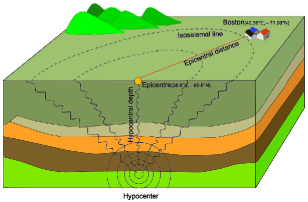
Figure 6: An illustration of the earthquake intensity data.

To transfer such multi-classification task into the binary classification setting considered in this paper, we set the labels lying in 1 to 4 as the positive class, while set the other labels lying in 5 to 12 as the negative class, mainly according to the damage extent of the earthquake suggested by the referred website. Moreover, we removed those incomplete records with missing labels. After such preprocessing, there are total 8,173 effective records. The settings of this experiment were similar to those on the UCI data sets. The classification accuracies of all algorithms are shown in Table VI.

From Table VI, the proposed boosting method with a suitable dictionary is generally better than the other state-of-the-art methods including two SVM methods, random forest, AdaBoost, and FPC. Moreover, the performance of the proposed boosting method with the polynomial kernel in this experiment is the best one among the used dictionaries.

TABLE VI: Test accuracies (in percentages) on the earthquake intensity data set, where the first four columns present the results of the proposed FCGBoosting over four differen types of dictionaries. The best and second results are marked in red and blue color, respectively.

Algorithm	FCGBoost-Gauss	FCGBoost-Poly	FCGBoost-Sigmoid	FCGBoost-ReLU	SVM-RBF	SVM-Poly	FPC	RF	AdaBoost
Test Acc. (%)	78.93	80.48	79.27	80.38	80.37	73.92	80.16	74.51	75.80

VI Proofs

In this section, we prove Theorem 1 and Theorem 2 by developing a novel concentration inequality associated with the squared hinge, a fast numerical convergence rate for FCGBoosting, and some standard error analysis techniques in [37, 25]. Throughout the proofs, we will omit the subscript of $\phi_{h^{2}}$ for simplicity, and denote $\phi$ as the squared hinge loss.

VI-A Concentration inequality with squared hinge loss

Denote by ${\cal E}(f):={\cal E}^{\phi}(f):=\int_{Z}\phi(yf(x))d\rho$ and ${\cal E}_{D}(f):={\cal E}_{D}^{\phi}(f):=\frac{1}{m}\sum_{i=1}^{m}\phi(y_{i}f(x_{i}))$ the expectation risk and empirical risk, respectively. Let

$$f_{\rho}(x):=\arg\min_{t\in\mathbb{R}}\int_{Y}\phi(yt)d\rho(y|x),$$

be the regression regression minimizing ${\cal E}(f)$. Since $\phi$ is the squared hinge loss, it can be found in [3] that

$$f_{\rho}(x)=2\eta(x)-1.$$ (7)

Our aim is to derive a learning rate for the generalization error $\mathcal{E}(f)-\mathcal{E}(f_{\rho}).$ Noting that the squared hinge loss $\phi$ is of quadratic type, we have [3, Lemma 7] (see also [25])

$$\frac{1}{2}\|f-f_{\rho}\|_{\rho}^{2}\leq\mathcal{E}(f)-\mathcal{E}(f_{\rho})\leq\|f-f_{\rho}\|_{\rho}^{2},\quad\forall f\in L_{\rho_{X}}^{2},$$ (8)

where $L_{\rho_{X}}^{2}$ denotes the space of $\rho_{X}$ square integrable functions endowed with norm $\|\cdot\|_{\rho}$. For $\mathcal{F}\in L^{1}(X)$, denote ${\cal N}_{1}(\epsilon,{\cal F})$ and ${\cal N}_{1}(\epsilon,{\cal F},x_{1}^{m})$ as the $\varepsilon$-covering number of $\mathcal{F}$ under the $L^{1}(X)$ and $\ell^{1}$ norms, respectively. The following concentration inequality is the main tool in our analysis.

Theorem 3.

Let $\mathcal{F}$ be a set of functions $f:\mathcal{X}\rightarrow\mathbb{R}$ satisfying $|f(x)|\leq 1,\forall x\in{\cal X}.$ Then for arbitrary $\beta>0$ and $f\in\mathcal{F}$, with confidence at least $1-\delta$, there holds

$$\mathcal{E}_{D}(f)-\mathcal{E}_{D}(f_{\rho})-(\mathcal{E}(f)-\mathcal{E}(f_{\rho}))$$ (9)

$$\leq \frac{17}{18}(\mathcal{E}(f)-\mathcal{E}(f_{\rho}))+\frac{1211}{m}\log\frac{1}{\delta}+\frac{4\beta}{9}$$

$$+ \frac{1164}{m}\exp\left(-\frac{\beta m}{654}\right)\mathbb{E}{\cal N}_{1}(\frac{\beta}{70},{\cal F},x_{1}^{m}).$$

It should be mentioned that a similar concentration inequality for the square loss is proved in [16, Theorem 11.4]. In [42], a more general concentration inequality associated with the $L^{\infty}$ covering number was presented for any bounded loss. Since we do not impose any bounded assumption on $f_{D,k}$, it is difficult to derive an $L^{\infty}$ covering number estimates for the hypothesis space of FCGBoosting. Under this circumstance, a concentration inequality presented in Theorem 3 is highly desired.

Let ${\cal F}$ be a set of functions $f:\mathbb{R}^{d}\rightarrow[-1,1]$. For $\varepsilon>0$ and $f\in\mathcal{F}$,

$$h_{f}(z)=\phi(yf(x))-\phi(yf_{\rho}(x))$$

and

$$v_{f,\varepsilon}(z)=\frac{h_{f}(z)-\mathbb{E}h_{f}}{\varepsilon+\mathbb{E}h_{f}}.$$

Denote

$$\mathcal{H}:=\{h_{f}:f\in\mathcal{F}\},\qquad\mathcal{V}_{\varepsilon}:=\{v_{f,\varepsilon}:f\in\mathcal{F}\}.$$

By the definition of $h_{f}$, one has

$${\cal E}(f)-{\cal E}(f_{\rho})=\mathbb{E}h_{f},\ {\cal E}_{D}(f)-{\cal E}_{D}(f_{\rho})=\frac{1}{m}\sum_{i=1}^{m}h_{f}(z_{i}).$$ (10)

One of the most important step-stones of our proof is the following relation between variance and expectation, which can be found in [3, Lemma 7 and Table 1].

$$\mathbb{E}h_{f}^{2}(z)\leq 32\mathbb{E}h_{f}(z).$$ (11)

To derive another tool, we recall a classical concentration inequality shown in the following lemma [16, Theorem 11.6].

Lemma 1.

Let ${\cal G}$ be a set of functions $g:\mathbb{R}^{d}\rightarrow[-B,B]$ and $\xi,\xi_{1},\ldots,\xi_{m}$ be i.i.d. $\mathbb{R}^{d}$-valued random variables. Assume $\alpha>0$, $0<\epsilon<1$, and $m\geq 1$. Then

$$\mathbb{P}\left\{\sup_{g\in{\cal G}}\frac{\frac{1}{m}\sum_{i=1}^{m}g(\xi_{i})-\mathbb{E}g(\xi)}{\alpha+\frac{1}{m}\sum_{i=1}^{m}g(\xi_{i})+\mathbb{E}g(\xi)}>\epsilon\right\}$$

$$\leq 4\mathbb{E}{\cal N}_{1}(\frac{\alpha\epsilon}{5},{\cal G},\xi_{1}^{m})\exp\left(-\frac{3\epsilon^{2}\alpha m}{40B}\right).$$

Based on Lemma 1, we can derive the following bound for $v_{f,\varepsilon}\in\mathcal{V}_{\varepsilon}$ easily.

Lemma 2.

For arbitrary $\beta,\varepsilon>0$ and $f\in\mathcal{F}$,

$$\mathbb{E}\left[\frac{1}{m}\sum_{i=1}^{m}v_{f,\varepsilon}(z_{i})\right]\leq\frac{\mathbb{E}h_{f}}{3\varepsilon}$$

$$+ \frac{\beta}{6\varepsilon}+\frac{436}{m\varepsilon}\exp\left(-\frac{\beta m}{654}\right)\mathbb{E}{\cal N}_{1}(\frac{\beta}{35},{\cal H},z_{1}^{m}).$$

Proof:

Since $|h_{f}(z)|\leq 4$, for $\varepsilon=1/7$, it follows from Lemma 1 with $\mathcal{G}=\mathcal{H}$ and $B=4$ that with confidence

$$1-4\mathbb{E}{\cal N}_{1}(\frac{\alpha}{35},{\cal H},z_{1}^{m})\exp\left(-\frac{3\alpha m}{1960}\right),$$

for all $h_{f}\in\mathcal{H}$, there holds

$$\frac{1}{m}\sum_{i=1}^{m}6h_{f}(z_{i})-8\mathbb{E}h_{f}(z)\leq\alpha.$$

For arbitrary $\beta\geq 0$ and $f\in\mathcal{F}$, if $\frac{6}{m}\sum_{i=1}^{m}h_{f}(z_{i})-8\mathbb{E}h_{f}(z)\geq 0$, we apply the formula

$$\mathbb{E}[\xi]=\int_{0}^{\infty}\mathbb{P}\left[\xi>t\right]dt$$ (12)

and obtain

$$\mathbb{E}\left[\frac{6}{m}\sum_{i=1}^{m}h_{f}(z_{i})-8\mathbb{E}h_{f}(z)\right]\leq\beta$$

$$+ 4\int_{\beta}^{\infty}\mathbb{E}{\cal N}_{1}(\frac{\alpha}{35},{\cal H},z_{1}^{m})\exp\left(-\frac{3\alpha m}{1960}\right)d\alpha$$

$$\leq \beta+4\mathbb{E}{\cal N}_{1}(\frac{\beta}{35},{\cal H},z_{1}^{m})\int_{\beta}^{\infty}\exp\left(-\frac{3\alpha m}{1960}\right)d\alpha$$

$$\leq \beta+\frac{2616}{m}\exp\left(-\frac{\beta m}{654}\right)\mathbb{E}{\cal N}_{1}(\frac{\beta}{35},{\cal H},z_{1}^{m}).$$

If $\frac{6}{m}\sum_{i=1}^{m}h_{f}(z_{i})-8\mathbb{E}h_{f}(z)<0$, the above estimate also holds trivially. Then for arbitrary $\varepsilon>0$ and $f\in\mathcal{F}$, it follows from the above estimate that

$$\mathbb{E}[\frac{1}{m}\sum_{i=1}^{m}v_{f,\varepsilon}(z_{i})]\leq\frac{2\mathbb{E}[h_{f}]+\mathbb{E}\left[\frac{6}{m}\sum_{i=1}^{m}h_{f}(z_{i})-8\mathbb{E}h_{f}(z)\right]}{6\varepsilon}$$

$$\leq\frac{1}{6\varepsilon}\left(2\mathbb{E}h_{f}+\beta+\frac{2616}{m}\exp\left(-\frac{\beta m}{654}\right)\mathbb{E}{\cal N}_{1}(\frac{\beta}{35},{\cal H},z_{1}^{m})\right).$$

This completes the proof of Lemma 2. ∎

The third tool of our proof is a simplified Talagrand’s inequality, which can be easily deduced from Theorem 7.5 and Lemma 7.6 in [37].

Lemma 3.

Let $\varepsilon>0$, $B\geq 0$ and $\sigma\geq 0$ be constants such that $\mathbb{E}[v_{f,\varepsilon}^{2}]\leq\sigma^{2}$ and $\|v_{f,\varepsilon}\|_{\infty}\leq B$ for all $v_{f,\epsilon}\in\mathcal{V}_{\epsilon}$. Then, for any $\tau>0$, $\gamma>0$ and $f\in\mathcal{F}$, with confidence $1-e^{-\tau}$, there holds

$$\sup_{v_{f,\varepsilon}\in\mathcal{V}_{\varepsilon}}\frac{1}{m}\sum_{i=1}^{m}v_{f,\varepsilon}(z_{i})\leq\sqrt{\frac{2\tau\sigma^{2}}{m}}+\left(\frac{2}{3}+\frac{1}{\gamma}\right)\frac{\tau B}{m}$$

$$+(1+\gamma)\mathbb{E}\left[\sup_{v_{f,\varepsilon}\in\mathcal{V}_{\varepsilon}}\frac{1}{m}\sum_{i=1}^{m}v_{f,\varepsilon}(z_{i})\right].$$

With these tools, we are now in the position to prove Theorem 3.

Proof:

For arbitrary $f\in\mathcal{F}$, we have $\|h_{f}\|_{\infty}\leq 4$ and $\|h_{f}-\mathbb{E}h_{f}\|_{\infty}\leq 8$. Let $\varepsilon\geq 2\inf_{f\in\mathcal{F}}\mathbb{E}[h_{f}]$. Then for arbitrary $v_{f,\varepsilon}\in\mathcal{V}_{\varepsilon}$, there exists an $f\in\mathcal{F}$ such that $v_{f,\varepsilon}=\frac{h_{f}-\mathbb{E}[h_{f}]}{\mathbb{E}[h_{f}]+\varepsilon}$. Then, we get from (11) that

$$\|v_{f,\varepsilon}\|_{\infty}\leq\frac{8}{\varepsilon}=:B,$$ (13)

and

$$\mathbb{E}[v^{2}_{f,\varepsilon}]\leq\frac{\mathbb{E}[h_{f}^{2}]}{(\mathbb{E}[h_{f}]+\varepsilon)^{2}}\leq\frac{32\mathbb{E}[h_{f}]}{(\mathbb{E}[h_{f}]+\varepsilon)^{2}}\leq\frac{16}{\varepsilon}.$$ (14)

Then Lemma 3 with $\gamma=1/3$ and $\varepsilon\geq\inf_{f\in\mathcal{F}}\mathbb{E}[h_{f}]$, Lemma 2, (13) and (14) that with confidence at least $1-e^{-\tau}$, for any $f\in\mathcal{F}$, there holds

$$\frac{1}{m}\sum_{i=1}^{m}v_{f,\varepsilon}(z_{i})\leq\sqrt{\frac{32\tau}{m\varepsilon}}+\frac{88\tau}{3m\varepsilon}+\frac{4}{9\varepsilon}\mathbb{E}[h_{f}]$$

$$+ \frac{2\beta}{9\varepsilon}+\frac{582}{m\varepsilon}\exp\left(-\frac{\beta m}{654}\right)\mathbb{E}{\cal N}_{1}(\frac{\beta}{35},{\cal H},z_{1}^{m}).$$

For arbitrary $f\in\mathcal{F}$, set $\tau=\log\frac{1}{\delta}$ and $\varepsilon=\mathcal{E}(f)-\mathcal{E}(f_{\rho})\geq\inf_{f\in\mathcal{F}}\mathbb{E}[h_{f}]$. It follows from (10) that , with confidence $1-\delta$, there holds

$$\mathcal{E}_{D}(f)-\mathcal{E}_{D}(f_{\rho})-(\mathcal{E}(f)-\mathcal{E}(f_{\rho}))$$

$$\leq \frac{8}{9}\mathbb{E}[h_{f}]+\sqrt{\frac{128(\mathcal{E}(f)-\mathcal{E}(f_{\rho}))}{m}\log\frac{1}{\delta}}+\frac{176}{3m}\log\frac{1}{\delta}$$

$$+ \frac{4\beta}{9}+\frac{1164}{m}\exp\left(-\frac{\beta m}{654}\right)\mathbb{E}{\cal N}_{1}(\frac{\beta}{35},{\cal H},z_{1}^{m}).$$

For arbitrary $h_{f_{1}},h_{f_{2}}\in\mathcal{H}$, we have

$$\|h_{f_{1}}-h_{f_{2}}\|_{\ell^{1}}=\|\phi(yf_{1})-\phi(yf_{2})\|_{\ell^{1}}\leq 2\|f_{1}-f_{2}\|_{\ell^{1}},$$

Then,

$$\mathbb{E}{\cal N}_{1}(\frac{\beta}{35},{\cal H},z_{1}^{m})\leq\mathbb{E}{\cal N}_{1}(\frac{\beta}{70},{\cal F},x_{1}^{m}).$$

Noting further that the element inequality $\sqrt{ab}\leq\frac{1}{2}(a+b)$ for $a,b>0$ yields

$$\sqrt{\frac{64(\mathcal{E}(f)-\mathcal{E}(f_{\rho}))}{m}\log\frac{1}{\delta}}\leq\frac{1}{18}(\mathcal{E}(f)-\mathcal{E}(f_{\rho}))+\frac{1152}{m}\log\frac{1}{\delta}.$$

This proves (9) and completes the proof of Theorem 3. ∎

VI-B Numerical convergence without boundedness assumption

In this part, we show the fast convergence rate of FCGBoosting without imposing any boundedness assumption. Our proof is motivated by [33] by taking the special property of the squared hinge. The following numerical convergence rate is another main tool in our proof.

Proposition 1.

For arbitrary $h\in\mathrm{span}{\cal G}_{n}$, we have

$$\mathcal{E}_{D}(f_{D,k})-\mathcal{E}_{D}(h)\leq\frac{4\|h\|_{\ell^{1}}^{2}}{k}.$$ (15)

It can be found in [2] and Proposition 1 that the numerical convergence rates for FCGBoosting are the same for the square loss and squared hinge loss. To prove the above proposition, we need the following lemma, which was proved in [33, Lemma B.2].

Lemma 4.

Let $c>0$ and let $\gamma_{0},\gamma_{1},\ldots$ be a sequence such that $\gamma_{t+1}\leq\gamma_{t}-c\gamma_{t}^{2}$ for all $t$. Let $\epsilon$ be a positive scalar and $k$ be a positive integer such that $k\geq\lceil\frac{1}{c\epsilon}\rceil$. Then $\gamma_{k}\leq\epsilon$.

Based on this lemma, we estimate the upper bound of ${\cal H}(D,k,h)$ in the following proposition. Similar results can be found in [33, Theorem 2.7] for the general smooth type loss functions. We provide its proof here for the sake of completeness.

Proof of Proposition 1.

Let $h=\sum_{j=1}^{n}\alpha_{j}g_{j}$ be an arbitrary function in $\mathrm{span}{\cal G}_{n}$. For $\alpha=(\alpha_{1},\dots,\alpha_{n})^{T}$, let $V:=V_{\alpha}:=\mathrm{supp}(\alpha)$ be the support of $\alpha$, which implies

$$\alpha_{j}=0,\ j\in V^{c}.$$ (16)

By Algorithm 1,

$${\cal E}_{D}(f_{D,k+1}) =\min_{\mathrm{supp}(f)={\cal T}^{k+1}}{\cal E}_{D}(f)$$

$$\leq\min_{j\in V}\min_{\eta}{\cal E}_{D}(f_{D,k}+\eta\cdot\mathrm{sgn}(h_{j})g_{j}).$$ (17)

By the Lipschitz continuity of $\phi^{\prime}$ with the Lipschtz constant $L=2$ and $\|g_{j}\|_{\infty}\leq 1$, [33, Lemma B.1] (see also[29]) shows

$${\cal E}_{D}(f_{D,k}+\eta\mathrm{sgn}(h_{j})g_{j})$$

$$\leq{\cal E}_{D}(f_{D,k})+\eta\mathrm{sgn}(h_{j})\langle\nabla{\cal E}_{D}(f_{D,k}),g_{j}\rangle+\eta^{2}$$

$$=:E_{j}(\eta)$$

for any $\eta\in\mathbb{R}$ and $j\in V$. Let $s:=\sum_{j\in V}|\alpha_{j}|=\|h\|_{\ell^{1}}$, then

$$s\min_{j\in V}E_{j}(\eta)\leq\sum_{j\in V}|\alpha_{j}|E_{j}(\eta)$$

$$=s{\cal E}_{D}(f_{D,k})+\eta\sum_{j\in V}\alpha_{j}\langle\nabla{\cal E}_{D}(f_{D,k}),g_{j}\rangle+s\eta^{2}.$$ (18)

Since ${\cal E}_{D}(f_{D,k})=\min_{\mathrm{supp}(f)={\cal T}^{k}}{\cal E}_{D}(f)$, and $f_{D,k}=\sum_{j=1}^{n}\beta_{j}^{k}g_{j}$, there holds

$$\langle\nabla{\cal E}_{D}(f_{D,k}),g_{j}\rangle=0,\ \forall j\in{\cal T}^{k},$$ (19)

and $\beta_{j}^{k}=0$ for any $j\in({\cal T}^{k})^{c}$. Thus,

$$\sum_{j\in V}\alpha_{j}\langle\nabla{\cal E}_{D}(f_{D,k}),g_{j}\rangle =\sum_{j\in V\backslash{\cal T}^{k}}\alpha_{j}\langle\nabla{\cal E}_{D}(f_{D,k}),g_{j}\rangle$$

$$=\sum_{j\in V\backslash{\cal T}^{k}}(\alpha_{j}-\beta_{j}^{k})\langle\nabla{\cal E}_{D}(f_{D,k}),g_{j}\rangle$$

$$=\sum_{j\in V\cup{\cal T}^{k}}(\alpha_{j}-\beta_{j}^{k})\langle\nabla{\cal E}_{D}(f_{D,k}),g_{j}\rangle$$

$$=\langle\nabla{\cal E}_{D}(f_{D,k}),h-f_{D,k}\rangle,$$ (20)

where the first equality holds for (19), the second equality holds for $\beta_{j}^{k}=0,\forall j\in({\cal T}^{k})^{c}$, the third equality holds for $\langle\nabla{\cal E}_{D}(f_{D,k}),g_{j}\rangle=0,\forall j\in{\cal T}^{k}$, and the final equality holds for $\alpha_{j}=\beta_{j}^{k}=0,\forall j\in(V\cup{\cal T}^{k})^{c}$. Furthermore, by the convexity of $\phi$, there holds

$${\cal E}_{D}(h)-{\cal E}_{D}(f_{D,k})\geq\langle\nabla{\cal E}_{D}(f_{D,k}),h-f_{D,k}\rangle.$$ (21)

Thus, by (17), (18), (20) and (21), there holds

$$s{\cal E}_{D}(f_{D,k+1})\leq s{\cal E}_{D}(f_{D,k})-\eta({\cal E}_{D}(f_{D,k})-{\cal E}_{D}(h))+s\eta^{2}$$

for any $\eta\in\mathbb{R}$. Taking $\eta=\frac{{\cal E}_{D}(f_{D,k})-{\cal E}_{D}(h)}{2s}$, the above inequality yields

$${\cal E}_{D}(f_{D,k+1}) \leq{\cal E}_{D}(f_{D,k})-\frac{({\cal E}_{D}(f_{D,k})-{\cal E}_{D}(h))^{2}}{4\|h\|_{\ell^{1}}^{2}}.$$

Denote $\epsilon_{k}={\cal E}_{D}(f_{D,k})-{\cal E}_{D}(h)$. The above inequality implies

$$\epsilon_{k+1}\leq\epsilon_{k}-\frac{\epsilon_{k}^{2}}{4\|h\|_{\ell^{1}}^{2}}.$$

Then Proposition 1 follows from Lemma 4. ∎

VI-C Learning rate analysis

Based on Theorem 3 and Proposition 1, we are in a position to prove the following theorem, which is a key stone to prove Theorems 1 and 2.

Theorem 4.

Let ${\cal G}_{n}:=\{g_{j}\}_{j=1}^{n}$ be a set of dictionaries with $n\sim m^{a}$ for some $a\geq 1$. Let $f_{D,k}$ be the predictor of Algorithm 1 after $k$ running iterations. If Assumption 1 holds, then for all $k\in\mathbb{N}$, with confidence at least $1-\delta$, there holds

$${\cal E}(\pi f_{D,k})-{\cal E}(f_{\rho})\leq\tilde{C}\left(n^{-2r}+k^{-1}+\frac{k\log m}{m}\log\frac{2}{\delta}\right).$$ (22)

where $\pi t=\min\{1,|t|\}\cdot\mathrm{sgn}(t)$ denotes the truncation of $t\in\mathbb{R}$ to $[-1,1]$ and $\tilde{C}$ is a constant depending only on $C_{1}$, $C_{2}$ and $a$, whose concrete value will be given in the proof.

The proof idea is somewhat standard [24, 25] which devotes to decomposing the generalization error into three terms: approximation error, sample error and hypothesis error. The approximation error can be derived from Assumption 1 and (8), the hypotheses error can be deduced from Proposition 1 and the sample error error can be derived using the concentration inequality in Theorem 3 and a covering number estimate of the hypothesis space.

Given any set $\Lambda\subset{\cal G}_{n},$ we define ${\cal J}_{\Lambda}:=\mathrm{span}\{g:g\in\Lambda\}$ and denote by $\pi{\cal J}_{\Lambda}:=\{\pi f:f\in{\cal J}_{\Lambda}\}$ the set of all truncations of the elements of ${\cal J}_{\Lambda}$. We then define

$${\cal F}_{k}:=\bigcup_{\Lambda\subset{\cal G}_{n},\sharp(\Lambda)\leq k}\pi{\cal J}_{\Lambda},$$ (23)

where $\sharp(\Lambda)$ represents the cardinality of set $\Lambda$ and $\pi f(x)=\min\{1,|f(x)|\}\cdot\mathrm{sgn}(f(x))$ is the truncation operator on $f(x)$ to $[-1,1]$. Due to [2, Lemma 3.3] with $B=1$, there holds

$${\cal N}_{1}(\epsilon,{\cal F}_{k})\leq 3m^{ak}\left(\frac{2e}{\epsilon}\log\frac{3e}{\epsilon}\right)^{k+1}.$$

Noting further $\sup_{x_{1}^{m}}{\cal N}_{1}(\epsilon,{\cal F}_{k},x_{1}^{m})\leq{\cal N}_{1}(\epsilon,{\cal F}_{k})$, we have the following covering number estimates.

Lemma 5.

Let ${\cal F}_{k}$ be defined as in (23). Assume that $n\sim m^{a}$ for some $a\geq 1$. Then for any probability measure $v$, for any $\epsilon>0$, we have the following $L_{1}$ empirical covering number estimate of ${\cal F}_{k}$

$$\sup_{x_{1}^{m}}{\cal N}_{1}(\epsilon,{\cal F}_{k},x_{1}^{m})\leq 3m^{ak}\left(\frac{2e}{\epsilon}\log\frac{3e}{\epsilon}\right)^{k+1}.$$ (24)

With these helps, we prove Theorem 4 as follows.

Proof:

Since $y=\{-1,1\}$, we have

$${\cal E}_{D}(\pi f_{D,k})\leq{\cal E}_{D}(f_{D,k}).$$ (25)

Then for arbitrary $h\in\mathrm{span}{\cal G}_{n}$, there holds

$${\cal E}(\pi f_{D,k})-{\cal E}(f_{\rho})$$ (26)

$$\leq{\cal A}({\cal G}_{n},h)+{\cal H}(D,k,h)+{\cal S}_{D}(h)-S_{D}(\pi f_{D,k}),$$

where

$${\cal A}({\cal G}_{n},h):={\cal E}(h)-{\cal E}(f_{\rho}),$$

$${\cal H}(D,k,h):={\cal E}_{D}(f_{D,k})-{\cal E}_{D}(h),$$

$${\cal S}_{D}(f):=({\cal E}_{D}(f)-{\cal E}_{D}(f_{\rho}))-({\cal E}(f)-{\cal E}(f_{\rho}))$$

are the approximation, hypothesis and sample errors, respectively. Due to Assumption 1, (7), (8) and $\|f\|_{\rho}\leq\|f\|_{\infty}$, we can get the following approximation error estimate directly.

$${\cal A}({\cal G}_{n},h_{0})\leq C_{1}^{2}n^{-2r},\ \text{and}\ \|h_{0}\|_{\ell^{1}}\leq C_{2}.$$ (27)

Furthermore, Proposition 1 shows

$$\mathcal{H}(D,k,h)\leq\frac{4\|h\|_{\ell^{1}}^{2}}{k}.$$ (28)

The only thing remainder is to bound the sample error ${\cal S}_{D}(h)$ and $-S_{D}(\pi f_{D,k})$. The former is pretty standard, we refer the readers to [34, 25] (with a slight change of constant) that with confidence $1-\delta/2$, there holds,

$${\cal S}_{D}(h) \leq\frac{4(B_{0}+1)^{2}\log\frac{2}{\delta}}{3m}$$ (29)

$$+2(B_{0}+1)\|h-f_{\rho}\|_{\rho}\sqrt{\frac{2\log\frac{2}{\delta}}{m}},$$

where $B_{0}:=\max\{\|h\|_{\infty},1\}$. Now, we turn to bound $-S_{D}(\pi f_{D,k})$. From Theorem 3 with $\mathcal{F}=\mathcal{F}_{k}$, we have for arbitrary $\beta>0$, with confidence $1-\delta/2$

$$-S_{D}(\pi f_{D,k}) \leq\frac{17}{18}(\mathcal{E}(\pi f_{D,k})-\mathcal{E}(f_{\rho}))+\frac{1211}{m}\log\frac{2}{\delta}$$ (30)

$$+\frac{4\beta}{9}+\frac{1164}{m}\exp\left(-\frac{\beta m}{654}\right)\mathbb{E}{\cal N}_{1}(\frac{\beta}{70},{\cal F}_{k},x_{1}^{m}).$$

For $\beta\geq 1/m$, Lemma 5 implies

$$\frac{1164}{m}\exp\left(-\frac{\beta m}{654}\right)\mathbb{E}{\cal N}_{1}(\frac{\beta}{70},{\cal F}_{k},x_{1}^{m})$$

$$\leq \exp\left\{\log\left[3492m^{ak-1}(140em\log(210em))^{k+1}\right]-\frac{\beta m}{654}\right\}$$

$$\leq \exp\bigg{\{}\log(3492)+(ak-1)\log m+(k+1)\Big{[}\log(140e)$$

$$+ \log m+\log\log(210em)\Big{]}-\frac{\beta m}{654}\bigg{\}}$$

$$\leq \exp\Big{\{}\bar{C}ak\log m-\frac{\beta m}{654}\Big{\}},$$

where $\bar{C}\geq 1$ is an absolute constant. Setting $\beta=\frac{1308\bar{C}ak\log m}{m},$ we obtain from (30) that

$$-S_{D}(\pi f_{D,k})\leq\frac{17}{18}(\mathcal{E}(f)-\mathcal{E}(f_{\rho}))+\frac{\bar{C}_{1}ak\log m}{m}\log\frac{2}{\delta},$$ (31)

where we use

$$\exp\big{\{}-\bar{C}ak\log m\big{\}}\leq m^{-a\bar{C}k}\leq\frac{1}{m}$$

and $\bar{C}_{1}$ is an absolute constant. Plugging (31), (29), (28) and (27) into (26) and noting $\|h\|_{\infty}\leq\|h\|_{\ell^{1}}\leq C_{2}$, $\sqrt{ab}\leq\frac{1}{2}(a+b)$, we obtain that

$$\frac{1}{18}({\cal E}(\pi f_{D,k})-{\cal E}(f_{\rho}))\leq C_{1}^{2}n^{-2r}+\frac{4C_{2}^{2}}{k}$$

$$+ \frac{4(C_{2}+2)^{2}\log\frac{2}{\delta}}{3m}+(C_{2}+2)(C_{1}^{2}n^{-2r}+2m^{-1}\log\frac{2}{\delta})$$

$$+ \frac{\bar{C}_{1}ak\log m}{m}\log\frac{2}{\delta}$$

holds with confidence $1-\delta$. That is, with confidence $1-\delta$, there holds

$${\cal E}(\pi f_{D,k})-{\cal E}(f_{\rho})\leq\tilde{C}\left(n^{-2r}+k^{-1}+\frac{k\log m}{m}\log\frac{2}{\delta}\right)$$

where $\tilde{C}=18\max\{(C_{2}+3)C_{1}^{2},4C_{2}^{2},2(C_{2}+2)^{2}+2(C_{2}+2)+a\bar{C}_{1}\}$. This completes the proof of Theorem 4. ∎

Based on Theorem 4, we can prove Theorems 1 and 2 as follows.

Proof of Theorem 1.

By (22), if $n\sim m^{a}$ for $a\geq 1$, $r\geq\frac{1}{4a}$, and $k\sim\sqrt{\frac{m}{\log m}}$, then

$${\cal E}(\pi f_{D,k})-{\cal E}(f_{\rho})\leq C_{4}\left(\frac{m}{\log m}\right)^{-1/2}\log\frac{4}{\delta},$$ (32)

where $C_{4}$ is a positive constant independent of $\delta$ or $m$. Furthermore, by the comparison inequality established by [7], that is,

$${\cal R}(\mathrm{sgn}(f))-{\cal R}(f_{c})\leq C_{\phi}\sqrt{{\cal E}(f)-{\cal E}(f_{\rho})}$$ (33)

for some constant $C_{\phi}>0$. Thus, Theorem 1 follows from (32) and (33). ∎

VI-C1 Proof of Theorem 2

Proof.

The claim of this theorem is yielded by (32) and the comparison inequality under Assumption 2 ([3], [43], see also [37, Theorem 8.29]), saying that for arbitrary measurable function $f:X\rightarrow\mathbb{R}$, there holds

$${\cal R}(\mathrm{sgn}(f))-{\cal R}(f_{c})$$

$$\leq 2^{\frac{3q+4}{q+2}}(\hat{c}_{q})^{-\frac{q}{q+2}}C_{\phi,1}^{-\frac{q+1}{q+2}}\left({\cal E}(f)-{\cal E}(f_{\rho})\right)^{\frac{q+1}{q+2}},$$

where $C_{\phi,1}$ is a constant depending only on the loss $\phi$. Let $C_{5}=2^{\frac{3q+4}{q+2}}(\hat{c}_{q})^{-\frac{q}{q+2}}C_{\phi,1}^{-\frac{q+1}{q+2}}C_{3}^{\frac{q+1}{q+2}}$. This finishes the proof. ∎

VII Conclusion

Binary classification is a very significant problem in machine learning. In this paper, we propose an efficient boosting method, aiming to improve the classification accuracy and establish the theoretical generalization guarantee. We adopt the fully-corrective greedy update scheme to the boosting procedure, and then exploit the special form of the so-called squared hinge loss to establish its fast learning rates in the framework of statistical learning, under some regular assumptions. Certain efficient early stopping rule is also derived for the proposed boosting method. The toy simulations are implemented to verify the feasibility of the proposed method as well as our theoretical findings. Moreover, a series of UCI data experiments and a real earthquake intensity data experiment are provided to show the effectiveness of the proposed method, particularly, the classification accuracies can be improved via our proposed method with an appropriate dictionary. Some future work is how to adopt the tree structures as the dictionary into the proposed method and establish the associated theoretical generalization guarantees.

Appendix

Appendix A: ADMM for FCG subproblem with squared hinge

Note that in Algorithm 1, the fully-corrective greedy step (5) presented in the functional form is equivalent to the following optimization problem presented in the vector form, that is,

$$\beta^{*}= \arg\min_{\beta\in\mathbb{R}^{n}}\frac{1}{m}\sum_{i=1}^{m}\left(1-y_{i}\sum_{j=1}^{n}\beta_{j}g_{j}(x_{i})\right)_{+}^{2}$$ (34)

$$\text{subject to}\ \ \mathrm{supp}(\beta)\subset{\cal T}^{k},$$

where $(z)_{+}:=\max\{0,z\}$ for any $z\in\mathbb{R}$, and $\mathrm{supp}(\beta)$ denotes the support set of $\beta$, i.e., the nonzero set of $\beta$. Then $f_{D,k}=\sum_{j\in{\cal T}^{k}}\beta_{j}^{*}g_{j}$.

In the following, we describe how to adopt the alternating direction method of multipliers (ADMM) to fast solve the optimization problem (34). Let $s$ be the cardinality of the set ${\cal T}^{k}$, $u=\beta_{{\cal T}^{k}}$, $A\in\mathbb{R}^{m\times s}$ be a matrix induced by the input $\{x_{i}\}_{i=1}^{m}$ and the dictionaries selected in ${\cal T}^{k}$, i.e., $A_{ij}=g_{{\cal T}^{k}(j)}(x_{i})$, where ${\cal T}^{k}(j)$ represents the $j$-th component of the set ${\cal T}^{k}$ and $g_{{\cal T}^{k}(j)}$ represents the dictionary with the index ${\cal T}^{k}(j)$. Thus, the optimization problem (34) can be reformulated as the following,

$$u^{*}=\arg\min_{u\in\mathbb{R}^{s}}\frac{1}{m}\sum_{i=1}^{m}\left(1-y_{i}\sum_{j=1}^{s}A_{ij}u_{j}\right)_{+}^{2}.$$ (35)

First, we reformulate (35) as the following equivalent problem

$$\mathop{\mathrm{minimize}}_{u\in\mathbb{R}^{s},v\in\mathbb{R}^{m}}\quad f(v):=\frac{1}{m}\sum_{i=1}^{m}\left(1-y_{i}v_{i}\right)_{+}^{2}$$ (36)

$$\text{subject to}\quad v=Au.$$

Then its augmented Lagrangian function is

$${\cal L}_{\gamma}(u,v,w)=f(v)+\langle w,v-Au\rangle+\frac{\gamma}{2}\|v-Au\|_{2}^{2},$$ (37)

where $w\in\mathbb{R}^{m}$ is a multiplier variable, $\gamma>0$ is an augmented parameter.

Based on the above defined augmented Lagrangian function, the ADMM method for (35) can be described as follows: given the initialization $u^{0},v^{0},w^{0}$, for $t=1,2,\ldots,$
(a) update $u^{t}$ via proximal scheme: for some $\alpha>0$ (default $\alpha=1$),

$$u^{t}=\arg\min_{u\in\mathbb{R}^{s}}{\cal L}_{\gamma}(u,v^{t-1},w^{t-1})+\frac{\alpha}{2}\|u-u^{t-1}\|_{2}^{2},$$ (38)

which implies that

$$u^{t}=(\gamma A^{T}A+\alpha{\bf I})^{-1}\left(A^{T}(\gamma v^{t-1}+w^{t-1})+\alpha u^{t-1}\right).$$ (39)

(b) update $v^{t}$:

$$v^{t}=\arg\min_{v\in\mathbb{R}^{m}}\ {\cal L}_{\gamma}(u^{t},v,w^{t-1}).$$ (40)

From the above equation, the $v^{t}$-subproblem is separable and thus can be reduced to the following univariate optimization problem,

$$v_{i}^{t}=$$ (41)

$$\arg\min_{v_{i}\in\mathbb{R}}\left(1-y_{i}v_{i}\right)_{+}^{2}+\frac{m\gamma}{2}\left(v_{i}-\sum_{j=1}^{n}A_{ij}u_{i}^{t}+\gamma^{-1}w_{i}^{t-1}\right)^{2},$$

which has the closed form solution as shown in Lemma 6 in Appendix B.

In a summary, the specific procedure of ADMM for the FCG optimization is presented in Algorithm 2.

Algorithm 2 ADMM for FCG subproblem (34)

   Input: training sample set $D:=\{x_{i},y_{i}\}_{i=1}^{m}$, $X:=(x_{1},\ldots,x_{m})^{T}$, $y:=(y_{1},\ldots,y_{m})^{T}$, dictionaries $\{g_{j}\}_{j\in{\cal T}^{k}}$, and matrix $A\in\mathrm{R}^{m\times s}$ with $A_{ij}=g_{{\cal T}^{k}(j)}(x_{i})$, where $s:=|{\cal T}^{k}|$, i.e., the cardinality of set ${\cal T}^{k}$.

  Initialization:$u^{0}\in\mathbb{R}^{k}$, $v^{0}\in\mathbb{R}^{m}$, and $w^{0}\in\mathrm{null}(A^{T})$ (i.e., the null space of the transpose of matrix $A$, say, $w^{0}=0$).

   for $t=1,2,\ldots,$

    update $u^{t}$ via (39),

    update $v^{t}$ via (41),

    $w^{t}=w^{t-1}+\gamma(v^{t}-Au^{t})$.

  End until the stopping criterion satisfied.

   Output: $u^{t}$.

Appendix B. Closed form solution of proximal of squared hinge

Consider the following optimization problem

$$u^{*}=\arg\min_{u}g(u):=\left(\max\{0,1-a\cdot u\}\right)^{2}+\frac{\gamma}{2}(u-b)^{2},$$ (42)

where $\gamma>0$.

Lemma 6.

The optimal solution of the problem (42) is shown as follows

$$\mathrm{hinge}_{\gamma}^{2}(a,b)= \left\{\begin{array}[]{cl}b,&\ \mathrm{if}\ a=0,\\ \frac{2a+\gamma b}{2a^{2}+\gamma},&\mathrm{if}\ a\neq 0,ab<1\\ b,&\mathrm{if}\ a\neq 0,ab\geq 1.\end{array}\right.$$

Proof.

We consider the problem (42) respectively in the following three scenarios: (1) $a>0$, (2) $a=0$ and (3) $a<0$.

Case 1. $a>0$: In this case,

$$g(u)=\left\{\begin{array}[]{cl}(1-au)^{2}+\frac{\gamma}{2}(u-b)^{2},&u<a^{-1},\\ \frac{\gamma}{2}(u-b)^{2},&\mathrm{u\geq a^{-1}}.\end{array}\right.$$

It is easy to show that the solution of the problem is

$$u^{*}=\left\{\begin{array}[]{cl}\frac{2a+\gamma b}{2a^{2}+\gamma},&\ \mathrm{if}\ a>0\ \mathrm{and}\ b<a^{-1},\\ b,&\ \mathrm{if}\ a>0\ \mathrm{and}\ b\geq a^{-1}.\end{array}\right.$$ (45)

Case 2. $a=0$: It is obvious that

$$u^{*}=b.$$ (46)

Case 3. $a<0$: Similar to Case 1,

$$g(u)=\left\{\begin{array}[]{cl}(1-au)^{2}+\frac{\gamma}{2}(u-b)^{2},&u\geq a^{-1},\\ \frac{\gamma}{2}(u-b)^{2},&{u<a^{-1}}.\end{array}\right.$$

Similarly, it is easy to show that the solution of the problem is

$$u^{*}=\left\{\begin{array}[]{cl}\frac{2a+\gamma b}{2a^{2}+\gamma},&\ \mathrm{if}\ a<0\ \mathrm{and}\ b\geq a^{-1},\\ a^{-1},&\ \mathrm{if}\ a<0\ \mathrm{and}\ a^{-1}<b<a^{-1}-\gamma^{-1}a,\\ b,&\ \mathrm{if}\ a<0\ \mathrm{and}\ b<a^{-1}.\\ \end{array}\right.$$ (50)

Thus, we finish the proof of this lemma. ∎

References

- [1] A. Bagirov, C. Clausen, and M. Kohler. An boosting algorithm for estimation of a regression function. IEEE. Trans. Inform. Theory, 56:1417-1429, 2010.
- [2] A.R. Barron, A. Cohen, W. Dahmen, and R. A. Devore, Approximation and learning by greedy algorithms. Ann. Statist., 36(1): 64-94, 2008.
- [3] P. L. Bartlett, M.I. Jordan, and J.D. McAuliffe, Convexity, classification, and risk bounds. J. Amer. Statist. Assoc., 101(473): 138-156, 2006.
- [4] P. Bartlett, and M. Traskin. AdaBoost is consistent. J. Mach. Learn. Res., 8: 2347-2368, 2007.
- [5] L. Breiman. Random forests. Mach. Learn., 45: 5-32, 2001.
- [6] P. Buhlmann and B. Yu. Boosting with the loss: regression and classification. J. Amer. Statist. Assoc., 98: 324-339, 2003.
- [7] D.R. Chen, Q. Wu, Y.M. Ying and D.X. Zhou. Support vector machine soft margine classifiers: Error analysis. J. Mach. Learn. Res., 5: 1143-1175, 2004.
- [8] F. Cucker and D. X. Zhou. Learning Theory: an Approximation Theory Viewpoint. Cambridge University Press, Cambridge, 2007.
- [9] Y. Freund. Boosting a weak learning algorithm by majority. Inform. Comput., 121(2): 256-285, 1995.
- [10] Y. Freund and R. E. Schapire. A decision-theoretic generalization of on-line learning and an application to boosting. J. Comput. Syst. Sci., 55(1): 119-139, 1997.
- [11] J. Friedman, T. Hastie and R. Tibshirani. Additive logistic regression: a stastical view of boosting. Ann. Statist., 28(2): 337-407, 2000.
- [12] J. Friedman. Greedy function approximation: a gradient boosting machine. Ann. Statist., 29(5): 1189-1536, 2001.
- [13] D. Gabay and B. Mercier. A dual algorithm for the solution of nonlinear variational problems via finite-element approximations. Comput. Maths. with Appls., 2: 17-40, 1976.
- [14] T. Gao and D. Koller. Multiclass boosting with hinge loss based on output coding. ICML, Bellevue, WA, USA, 2011.
- [15] R. Glowinski and A. Marrocco. Approximation par éléments finis d’ordre un et résolution par pénalisation-dualité d’une classe de problèms non linéaires. RAIRO, R2: 41-76, 1975.
- [16] L. Gyrfi, M. Kohler, A. Krzyak and H. Walk. A Distribution-free Theory of Nonparametric Regression. Springer, New York, 2002.
- [17] T. Hastie, R. Tibshirani and J. Friedman. The Elements of Statistical Learning: Data mining, Inference and Prediction. Springer, New York, 2001.
- [18] T. Hastie, J. Taylor, R. Tibshirani and G. Walther, Forward stagewise regression and the monotone lasso. Electronic Journal of Statistics, 1: 1-29, 2007.
- [19] B. He and X. Yuan, On the O() convergence rate of Douglas-Rachford alternating direction method. SIAM J. Numer. Anal., 50(2): 700-709, 2012.
- [20] M. Jaggi. Revisiting Frank-Wolfe: Projection-free sparse convex optimization. ICML, Atlanta, Georgia, USA, 2013.
- [21] K. Janocha and W.M. Czarnecki. On loss functions for deep neural networks in classification. Schedae Informaticae, 25: 49-59, 2016.
- [22] R. Johnson and T. Zhang. Learning nonlinear functions using regularized greedy forest, IEEE Trans. Pattern Anal. Mach.Intel., 36(5): 942-954, 2014.
- [23] T. Kanamori, A. Takeda and T. Suzuki. A conjugate property between loss functions and uncertainty sets in classification problems. COLT, vol. 23, 29.1-29.3, 2012.
- [24] S. Lin, Y. Rong, X. Sun and Z. Xu. Learning capability of relaxed greedy algorithms. IEEE Trans. Neural Netw. & Learn. Syst. 24: 1598-1608, 2013.
- [25] S. B. Lin, J. Zeng and X. Chang. Learning rates for classification with Gaussian kernels. Neural Comput., 29: 3353-3380, 2017.
- [26] E. Livshits. Lower bounds for the rate of convergence of greedy algorithms. Izvestiya: Mathematics, 73: 1197-1215, 2009.
- [27] O. L. Mangasarian and D. R. Musicant. Lagrangian support vector machines. J. Mach. Learn. Res., 1: 161-177, 2001.
- [28] I. Mukherjee, C. Rudin and R. E. Schapire. The rate of convergence of AdaBoost. J. Mach. Learn. Res., 14(1): 2315-2347, 2013.
- [29] Y. Nestrov. Introductory Lectures on Convex Optimization. Springer Science & Business Media, volumn 87, 2004.
- [30] R.E. Schapire. The strength of weak learnability. Mach. Learn., 5(2): 197-227, 1990.
- [31] R.E. Schapire. The boosting approach to machine learning: An overview. in Nonlinear Estimation Classification, New York, NY, USA: Springer, 2003.
- [32] R. E. Schapire and Y. Freund. Boosting: Foundations and Algorithms. MIT Press, MIT, 2012.
- [33] S. Shalev-Shawartz, N. Srebro and T. Zhang. Trading accuracy for sparsity in optimization problems with sparsity constraints, SIAM J. OPTIM., 20(6): 2807-2832, 2010.
- [34] L. Shi, Y. Feng and D.X. Zhou. Concentration estimates for learning with regularizer and data dependent hypothesis spaces. Appl. Comput. Harmonic Anal., 31(2): 286-302, 2011.
- [35] J. Sochman and J. Malas. AdaBoost with totally corrective updates for fast face detection. In Proceedings of the 6th IEEE International Conference on Automatic Face and Gesture Recognition, Seoul, South Korea, 2004.
- [36] I. Steinwart and C. Scovel. Fast rates for support vector machines using Gaussian kernels. Ann. Statist., 35: 575-607, 2007.
- [37] I. Steinwart and A. Christmann. Support Vector Machines. Springer, New York, 2008.
- [38] V. Temlyakov. Greedy approximation. Acta Numer., 17:235-409, 2008.
- [39] J.A. Tropp and A. Gilbert. Signal recovery from random measurements via orthogonal matching pursuit. IEEE Trans. On Inform. Theory, 53(12): 4655-4666, 2007.
- [40] A. Tsybakov. Optimal aggregation of classifiers in statistical learning. Ann. Statist., 32: 575-607, 2004.
- [41] Y. Wang, X. Liao and S. Lin. Rescaled boosting in classification. IEEE Trans. Neural Netw. & Learn. Syst., 30(9): 2598-2610, 2019.
- [42] Q. Wu and D.X. Zhou. SVM soft margin classifier: linear programming versus quadratic programming. Neural Comput., 17: 1160-1187, 2005.
- [43] D. H. Xiang. Classification with gaussians and convex loss II: Improving error bounds by noise conditions. Sci. China Math., 54: 165-171, 2011.
- [44] J. Zeng, M. Wu, S.B. Lin and D.X. Zhou. Fast polynomial kernel classification for massive data. arXiv:1911.10558, 2019.
- [45] T. Zhang and B. Yu. Boosting with early stopping: convergence and consistency. Ann. Statis., 33:1538-1579, 2005.