Moving-Resting Process with Measurement Error in Animal Movement Modeling

Abstract.

Statistical modeling of animal movement is of critical importance. The continuous trajectory of an animal’s movements is only observed at discrete, often irregularly spaced time points. Most existing models cannot handle the unequal sampling interval naturally and/or do not allow inactivity periods such as resting or sleeping. The recently proposed moving-resting (MR) model is a Brownian motion governed by a telegraph process, which allows periods of inactivity in one state of the telegraph process. The MR model shows promise in modeling the movements of predators with long inactive periods such as many felids, but the lack of accommodation of measurement errors seriously prohibits its application in practice. Here we incorporate measurement errors in the MR model and derive basic properties of the model. Inferences are based on a composite likelihood using the Markov property of the chain composed by every other observed increments. The performance of the method is validated in finite sample simulation studies. Application to the movement data of a mountain lion in Wyoming illustrates the utility of the method.

Keywords: Composite likelihood; Dynamic programming; Markov process

1. Introduction

Statistical modeling of animal movement is of great importance in addressing fundamental questions about space use, movement, resource selection, and behavior in animal ecology (Hooten et al., 2017). The explosion of telemetric data on animal movement from the recent advancements in tracking and observation technologies presents countless opportunities and challenges (Cagnacci et al., 2010; Patterson et al., 2017). Telemetry devices, like Global Positioning System (GPS) receivers, can only determine an animal’s position at discrete moments in time so a continuous trajectory is never available. Programming the device to record at a very fast fix rate could approximate a continuous trajectory, but this is seldom done due to battery life limitations: it is very expensive to capture and collar an animal, so a long episodic time record is usually preferable to a highly detailed record, especially for animals that spend a great deal of time not moving around. GPS receivers often produce fixes at irregularly spaced time points, even if researchers program for regular intervals, due to environmental factors such as satellite communication issues or sky occlusion. As a result, discrete-time models such as the state space model (e.g., Jonsen et al., 2005; Patterson et al., 2008; Brett et al., 2012) are not realistic. Continuous-time models based on stochastic differential equations (SDE) (e.g., Preisler et al., 2004; Horne et al., 2007; Brillinger, 2010) can handle the irregular spacing naturally. Nonetheless, most existing work assumes perpetual motion and cannot accommodate periods of inactivity. On the time scale of most telemetry data, most animals alternate between periods of movement (foraging) and periods of inactivity (e.g., prey handling or rest Mashanova et al., 2010; Ueno et al., 2012; Jeschke, 2007). Realistic continuous-time models that accommodate inactive periods are needed.

The recently proposed moving-resting (MR) process by Yan et al. (2014) is a promising model to accommodate inactive periods. The MR process is a Brownian motion governed by a telegraph or on-off process (e.g., Zacks, 2004). Specifically, it allows an animal to alternate between a moving state, during which it moves in a Brownian motion (BM), and a resting state, during which it remains motionless. The switch between the two states is governed by a telegraph process, where the holding time (or duration) of each state is assumed to follow an exponential distribution. The memoryless holding time makes the underlying state process a continuous time Markov Chain. As a consequence, the MR process can be analyzed with the help of hidden Markov model (HMM) tools (Cappé et al., 2005). The MR process is a first step towards more realistic animal movement modeling with discretely observed telemetry data where the trajectories contain evident motionless segments. Implementation of likelihood based inferences for the MR process based on dynamic programming (Pozdnyakov et al., 2019) is publicly available in an R package smam (Hu et al., 2020b).

The MR model does not accommodate the measurement error or noise of telemetric devices, which is a major limitation in applying it to animal movement data. Adding measurement error to a Brownian motion model is not crucial as long as the noise is small in comparison to the total standard deviation of the increments of the Brownian motion between two consecutive time points (Pozdnyakov et al., 2014). In such cases, discarding the noise would not produce significant bias. The impact of the noise on inferences about MR processes, however, is much greater. For a given sequence of hidden states, the likelihood is a product of both densities and probabilities. With perfect instrumentation, if a sequence of observed locations are exactly the same, that is, there is no change in either the easting nor northing coordinates for a period of time resulting in a “flat” piece of trajectory, then the animal is known to be motionless over the time period spanned by the sequence. The likelihood contribution is the probability of staying in the motionless state instead of the density of the increment at zero. Adding even a tiny bit of noise would remove those flat pieces and, hence, cause drastic bias in the likelihood estimator of the parameters. One possible remedy is to round the observed coordinates, which enforces flat pieces. The number of such pieces, however, depends greatly on the rounding level, and there are no obvious rules to aid researchers in choosing best levels. A detailed illustration of the issue is given in Section 2.

Dealing with added noise in an MR process is challenging because it invalidates the Markov property of the joint location-state process. The transition density from one time point to the next can in principle be obtained from convolving the results for the MR process (Yan et al., 2014) with normally distributed noises, although computationally very intensive. A lack of Markov property of the joint location-state process means that the likelihood cannot be easily formed by multiplying these transition densities. Because the measurement errors are continuous, the dynamic programming tools of HMM based on a finite number of hidden states (Cappé et al., 2005) are not applicable. The generic simulation based inferences such as iterated filtering (Ionides et al., 2011, 2015) or particle Markov chain Monte Carlo (Andrieu et al., 2010), available in R package pomp (King et al., 2016), are not applicable to our investigation due to the complexity of the MR process with measurement error.

Our contribution in this paper is a toolbox for applying the MR process with measurement error to animal movement modeling. First, we show that discarding the measurement error, even tiny ones, causes severe bias in estimation, and that rounding does not provide any satisfactory solution. To make inferences for MR process with measurement error, we establish that, after thinning every other observation, the remaining observations are location-state Markov. This facilitates a composite likelihood which contains two true likelihood components, one based on odd-numbered observations and the other based on even-numbered observations. The true likelihood of each component is computed with dynamic programming. The variance of the maximum composite likelihood estimator can be estimated through parametric bootstrap. The validity of the approach is confirmed in a simulation study. We then apply the approach to model the movement data of a mountain lion in Wyoming, whose trajectory is known to have long inactive periods. Our methods are publicly available in an R package smam (Hu et al., 2020b) with efficient C++ code.

2. Moving-Resting Process

The MR process is a Brownian motion with an infinitesimal variance that is governed by an alternating renewal process with two different holding times. Let random variables $\{M_{i}\}_{i\geq 1}$ be independent exponential variables with rate $\lambda_{1}$, and $\{R_{i}\}_{i\geq 1}$ be independent exponential variables with rate $\lambda_{0}$. These are the holding times. There are two possible alternating sequences of the holding times, $(M_{1},R_{1},M_{2},R_{2},\dots)$ or $(R_{1},M_{1},R_{2},M_{2},\dots)$. Which one represents a particular realization depends on an initial distribution. A continuous time state process, $S(t)$, $t\geq 0$, takes only two values, 0 and 1, and it is defined by the holding times. In particular, for sequence $(M_{1},R_{1},M_{2},R_{2},\dots)$, if there exists $k\geq 0$ such that

$$\sum_{j=1}^{k}(M_{j}+R_{j})<t\mbox{ but }\sum_{j=1}^{k}(M_{j}+R_{j})+M_{k}\geq t,$$

then $S(t)=1$; otherwise, $S(t)=0$. For sequence $(R_{1},M_{1},R_{2},M_{2},\dots)$, if there exists $k\geq 0$ such that

$$\sum_{j=1}^{k}(R_{j}+M_{j})<t\mbox{ but }\sum_{j=1}^{k}(R_{j}+M_{j})+R_{k}\geq t,$$

then $S(t)=0$, otherwise, $S(t)=1$. It is well-known that the state process is stationary, if the initial probability of $\{S(0)=1\}$ is set as

$$p_{1}=\frac{\lambda_{0}}{\lambda_{0}+\lambda_{1}},$$

and the initial probability of $\{S(0)=0\}$ is set as $p_{0}=1-p_{1}$.

An MR process $X(t)$, $t\geq 0$, is defined by a stochastic differential equation

(1) $$\mathrm{d}X(t)=\begin{cases}\sigma\mathrm{d}B(t)&\quad\text{if }S(t)=1,\\ 0&\quad\text{if }S(t)=0,\end{cases}$$

where $B(t)$ is the standard Brownian motion, and $\sigma$ is a volatility parameter. It is important to note that $\{X(t)\}_{t\geq 0}$ itself is not Markov, but the location-state process $\{X(t),S(t)\}$ is a Markov process with stationary increments.

Properties and inferences of the MR process have been studied in Yan et al. (2014) and Pozdnyakov et al. (2019). A key element is the distribution of occupation times, that is, the total time spent in the moving state by time $t$

$$M(t)=\int_{0}^{t}S(s)\mathrm{d}s,$$

and the total time spent in the resting state $R(t)=t-M(t)$. Let ${P}_{i}(\cdot)$ be the conditional probability $\Pr(\cdot|S(0)=i)$. Zacks (2004) derived computationally efficient formulas for the following (defective) densities for $0<w<t$:

$$p_{11}(w,t)\mathrm{d}w ={P}_{1}(M(t)\in\mathrm{d}w,S(t)=1),$$

$$p_{10}(w,t)\mathrm{d}w ={P}_{1}(M(t)\in\mathrm{d}w,S(t)=0),$$

$$p_{01}(w,t)\mathrm{d}w ={P}_{0}(R(t)\in\mathrm{d}w,S(t)=1),$$

$$p_{00}(w,t)\mathrm{d}w ={P}_{0}(R(t)\in\mathrm{d}w,S(t)=0).$$

Having this at hand, one can derive the marginal distribution of the increment $X(t)-X(0)$. Without loss of generality, let $X(0)$ to be $0$, and $X(t)$ becomes the increment from time $0$ to time $t$. Then, the joint distribution of the increment $X(t)$ and $S(t)$, $t>0$, is

$${P}_{1}(X(t)\in\mathrm{d}x,S(t)=1) =h_{11}(x,t)\mathrm{d}x,$$

$${P}_{1}(X(t)\in\mathrm{d}x,S(t)=0) =h_{10}(x,t)\mathrm{d}x,$$

$${P}_{0}(X(t)\in\mathrm{d}x,S(t)=0) =h_{00}(x,t)\mathrm{d}x+e^{-\lambda_{0}t}\delta_{0}(x),$$

$${P}_{0}(X(t)\in\mathrm{d}x,S(t)=1) =h_{01}(x,t)\mathrm{d}x,$$

where $\delta_{0}(x)$ is the delta function with an atom at $0$, $x\in\mathbb{R}$, and $h_{ij}(x,t)$, $i,j\in\{0,1\}$, are functions derived in Yan et al. (2014):

$$h_{11}(x,t) =e^{-\lambda_{1}t}\phi(x;\sigma^{2}t)+\int_{0}^{t}\phi(x;\sigma^{2}w)p_{11}(w,t)\mathrm{d}w,$$

$$h_{10}(x,t) =\int_{0}^{t}\phi(x;\sigma^{2}w)p_{10}(w,t)\mathrm{d}w,$$

$$h_{00}(x,t) =\int_{0}^{t}\phi(x;\sigma^{2}(t-w))p_{00}(w,t)\mathrm{d}w,$$

$$h_{01}(x,t) =\int_{0}^{t}\phi(x;\sigma^{2}(t-w))p_{01}(w,t)\mathrm{d}w.$$

with $\phi(\cdot;\sigma^{2})$ being the density function of normal distribution $\mathrm{N}(0,\sigma^{2})$. The marginal distribution of increment $X(t)$ can be obtained by summing out $S(t)$ and $S(0)$, which forms the basis of the composite likelihood in Yan et al. (2014). The full maximum likelihood estimation based on dynamic programming was developed in Pozdnyakov et al. (2019).

For actual animal movement data, we never observe the exact values of $X(t)$ but only $X(t)$ with added measurement errors. For an MR process, the probability of observing a zero increment is strictly positive. Adding noise makes this probability zero. Rounding can help, but it is not trivial to come up with an appropriate rounding level. Figure 1 (upper left) shows the easting/northing coordinates in the Universal Transverse Mercator (UTM) coordinate system of a female mountain lion in 2012 in the Gros Ventre mountain range, Wyoming. The patterns of resting — places where both lines are more or less flat — and moving are readily apparent, which can hardly be captured by any existing model that assumes perpetual movements. The other three panels of Figure 1 show the coordinates of a simulated MR path without noise and with noise of two levels. The pattern is very similar to that in the upper left panel for the female mountain lion. The similarity is obvious, suggesting that an MR process might be a good model, but as shown next, ignoring the noise is disastrous in estimating the model parameters.

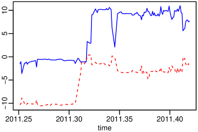
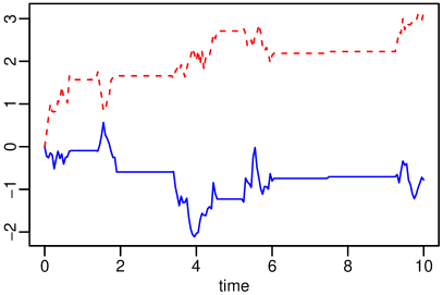
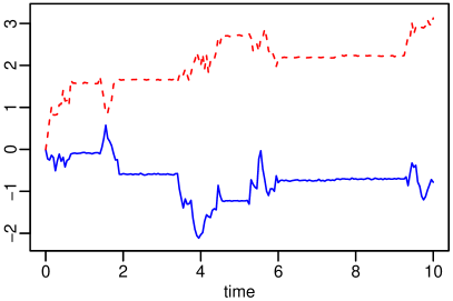
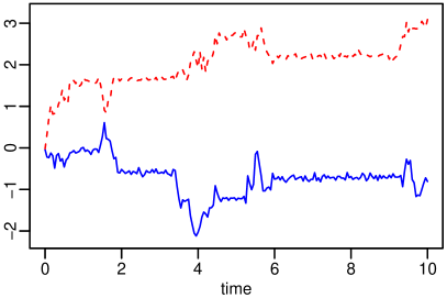
Figure 1. Upper left: Actual coordinates of a female mountain lion in a two-month period in 2012 in the Gros Ventre mountain range, Wyoming, with most observations separated by 8 hours. The x-axis is time in years. The y-axis is departure from the starting point. The solid blue line is UTM easting (km) and the dashed red line is UTM northing (km). Upper right: Coordinates of a realization from a two-dimensional MR process. The two coordinates are dependent because the straight line segments representing resting periods are shared. Bottom left: Coordinates of the same realization as in upper right panel after adding Gaussian noise with standard deviation 0.01 km. Bottom right: Coordinates of the same realization as in upper right panel after adding Gaussian noise with standard deviation 0.05km.

We demonstrate the impact of noise on estimation by a simulation study. Consider an MR process with parameters $\lambda_{1}=1\text{ hour}^{-1}$, $\lambda_{0}=0.5\text{ hour}^{-1}$, $\sigma=1\text{ km}/\text{hour}^{1/2}$. The measurement errors were independent Gaussian noise with standard deviation $0.05\text{ km}$ ($1/20$ of $\sigma$) and $0.01\text{ km}$ ($1/100$ of $\sigma$). The time intervals between consecutive observations was 5 hours. We generated 100 datasets, each with sampling horizon 1000 hours. The maximum likelihood estimates based on the MR process were obtained for dataset with and without noise, where for data with noise, three levels of rounding were considered, 10, 50, and 100 meters. Table 1 summarizes the parameter estimates based on the 100 replicates. When there was no noise, the point estimates were good, recovering the true parameters with high accuracy. For data with noise but no rounding, the optimization did not converge for most replications because of the Nelder-Mead simplex degeneracy (Nelder and Mead, 1965). With the help of various levels of rounding, the convergence percentage increases as the rounding becomes coarser, and the bias decreases but remain notable. This is true even for the cases with a noise standard deviation $0.01\text{ km}$. It is indeed unclear how to choose an appropriate rounding level. A practical model should handle the measurement errors directly.

Table 1. Summaries of the Influence of measurement error on MR process parameter estimation based on 100 replicates. The true parameters of the MR process were $\lambda_{1}=1\text{ hour}^{-1}$, $\lambda_{0}=0.5\text{ hour}^{-1}$, $\sigma=1\text{ km}/\text{hour}^{1/2}$. The measurement error was set as Gaussian noise with standard deviation (s.d.) $0.05$ and $0.01$. In each replicate, data were generated on a time horizon of $(0,500)$ with sampling interval 1. The mean and standard deviation of the point estimates, along with the convergence percentage of the optimizations under different setups are reported.

Gaussian noise	Rounding	Convergence	$\hat{\lambda}_{1}$		$\hat{\lambda}_{0}$		$\hat{\sigma}$
s.d. (km)	(km)	percentage (%)	mean	s.d.	mean	s.d.	mean	s.d
—	—	100	1.00	0.17	0.50	0.05	1.00	0.05
0.05	—	7	348.08	121.53	2.82	0.08	5.42	0.98
	0.01	6	304.83	127.91	2.80	0.08	5.05	1.10
	0.05	14	240.54	135.93	2.54	0.11	4.73	1.34
	0.10	33	128.79	91.36	2.06	0.12	3.94	1.36
0.01	—	5	409.34	148.78	2.42	0.07	5.90	1.07
	0.01	10	346.62	165.24	2.25	0.09	5.64	1.46
	0.05	100	3.65	4.26	1.01	0.16	1.06	0.24
	0.10	99	1.33	0.28	0.67	0.07	0.95	0.05

3. Moving-Resting Process with Measurement Error

Suppose the observations are recorded at times $t_{0}=0,t_{1},\dots,t_{n}$. Let $\{\epsilon_{k}\}_{k=0,\dots,n}$ be independent and identically normally distributed random variables with mean 0 and variance $\sigma_{\epsilon}^{2}$. An MR process with measurement error (MRME) $Z(t_{k})$, $k=0,1,\dots,n$, is the superimposition of a measurement error and the exact location:

(2) $$Z(t_{k})=X(t_{k})+\epsilon_{k},$$

where $X(\cdot)$ is an MR process in Equation (1), and $\epsilon_{k}$’s are independent $\mathrm{N}(0,\sigma_{\epsilon}^{2})$ noises.

Some properties of the process $\{Z(t_{k})\}_{k=0,\dots,n}$ are in order. Obviously, it is not Markov. Neither is the location-state process $\{Z(t_{k}),S(t_{k})\}_{k=0,\dots,n}$. To get a Markov process one might consider including the measurement errors. It is true that $\{Z(t_{k}),S(t_{k}),\epsilon_{k}\}_{k=0,\dots,n}$ is Markov. But the cardinality of hidden states $(S(t_{k}),\epsilon_{k})$ is a continuum in this case. This makes the dynamic programming approach for computing likelihood infeasible. To address this difficulty we suggest considering the process $\{Z(t_{2k})-Z(t_{2k-1}),S(t_{2k})\}_{k=1,\dots,[n/2]}$. The process is Markov, because the increment of the Brownian motion between times $t_{2k+1}$ and $t_{2k+2}$ and measurement errors $\epsilon_{2k+2}$ and $\epsilon_{2k+1}$ are independent of observations collected by time $t_{2k}$. Moreover, the process has a finite set of hidden states. This is an important property which is used to develop a forward algorithm for efficient computing of a composite likelihood in the next section. The conditional distribution of $(Z(t_{2k+2})-Z(t_{2k+1}),S(t_{2k+2}))$ (given the observations up to time $t_{2k}$) depends only on state $S(t_{2k})$.

Here we present our derivations for a one-dimensional case. The real-world animal movement data sets are two-dimensional. The formulas from below can be generalized to a $d$-dimensional case. The details are given in Appendix. All our simulations and data analysis are also performed using two-dimensional formulas.

First, let us calculate the marginal distribution of $Z(t)-Z(0)$ (the increment of one-dimensional $\{Z(v)\}_{v\geq 0}$ from time $0$ to time $t$). Consider

$$\Delta Z(t)=Z(t)-Z(0)=X(t)-X(0)+\xi(t),$$

where $\xi(t)\sim\mathrm{N}(0,2\sigma_{\epsilon}^{2})$ is independent of process $(X(\cdot),S(\cdot))$. Note that

$$Z(t_{2k+2})-Z(t_{2k+1})=X(t_{2k+2})-X(t_{2k+1})+\epsilon_{2k+2}-\epsilon_{2k+1},$$

and $(\epsilon_{2k+2}-\epsilon_{2k+1})\sim\mathrm{N}(0,2\sigma_{\epsilon}^{2})$. Without loss of generality, we assume that $X(0)=0$. Define

$$g_{ij}(z,t)={P}_{i}(\Delta Z(t)\in\mathrm{d}z,S(t)=j)/\mathrm{d}z,$$

where $i,j=\{1,0\}$. Then, we get that

$$g_{11}(z,t)\mathrm{d}z= {P}_{1}(\Delta Z(t)\in\mathrm{d}z,S(t)=1)$$

$$= \int_{\mathbb{R}}{P}_{1}(X(t)+\xi(t)\in\mathrm{d}z,S(t)=1,\xi(t)\in\mathrm{d}x)$$

$$= \int_{\mathbb{R}}{P}_{1}(X(t)\in\mathrm{d}z-x,S(t)=1)\phi(x;2\sigma_{\epsilon}^{2})\mathrm{d}x$$

$$= \int_{\mathbb{R}}h_{11}(z-x,t)\mathrm{d}z\phi(x;2\sigma_{\epsilon}^{2})\mathrm{d}x,$$

where, as before, $\phi(\cdot;\sigma^{2})$ is the density function of $\mathrm{N}(0,\sigma^{2})$. Similarly, one can get that

$$g_{10}(z,t)= \int_{\mathbb{R}}h_{10}(z-x,t)\phi(x;2\sigma_{\epsilon}^{2})\mathrm{d}x,$$

$$g_{01}(z,t)= \int_{\mathbb{R}}h_{01}(z-x,t)\phi(x;2\sigma_{\epsilon}^{2})\mathrm{d}x,$$

$$g_{00}(z,t)= \int_{\mathbb{R}}h_{00}(z-x,t)\phi(x;2\sigma_{\epsilon}^{2})\mathrm{d}x+e^{-\lambda_{0}t}\phi(z;2\sigma_{\epsilon}^{2}).$$

Next, let us denote

$$\tau_{ij}(t)={P}_{i}(S(t)=j).$$

It is easy to see

$$\tau_{01}(t) ={P}_{0}(S(t)=1)$$

$$=\sum_{n=0}^{\infty}\left[{P}\left(\sum_{k=1}^{n+1}R_{k}+\sum_{k=1}^{n}M_{k}\leq t\right)-{P}\left(\sum_{k=1}^{n+1}R_{k}+\sum_{k=1}^{n+1}M_{k}\leq t\right)\right]$$

$$=\sum_{n=0}^{\infty}H(t;n,\lambda_{1},n+1,\lambda_{0}),$$

where $\{M_{i}\}_{i\geq 1}$ and $\{R_{i}\}_{i\geq 1}$ are defined in Section 2, and a summation over an empty set is 0 and $H(t;a_{1},b_{1},a_{2},b_{2})$ is a special function involving convolutions of independent gamma variables studied by Hu et al. (2020a). Specifically, with $F(t;a_{1},b_{1},a_{2},b_{2})$ being the distribution function of the sum of two independent gamma variables with parameters $(a_{1},b_{1})$ and $(a_{2},b_{2})$, respectively, $H(t;a_{1},b_{1},a_{2},b_{2})=F(t;a_{1},b_{1},a_{2},b_{2})-F(t;a_{1}+1,b_{1},a_{2},b_{2})$ can be computed efficiently (Hu et al., 2020a, Lemma 1). Using similar techniques, we obtain that

$$\tau_{10}(t) =\sum_{n=0}^{\infty}H(t;n,\lambda_{0},n+1,\lambda_{1}),$$

$$\tau_{00}(t) =\sum_{n=0}^{\infty}H(t;n,\lambda_{0},n,\lambda_{1}),$$

$$\tau_{11}(t) =\sum_{n=0}^{\infty}H(t;n,\lambda_{1},n,\lambda_{0}).$$

Finally, we are ready to present the transition density at $(Z(t)-Z(u),S(t))$ given $S(0)$, where $0<u<t$, $Z(u)=X(u)+\xi(u)$, and $\xi(u)\sim\mathrm{N}(0,\sigma_{\epsilon}^{2})$ is independent of $\xi(t)$ and process $(X(\cdot),S(\cdot))$. Using the Markov property of the location-state process $(X(t)),S(t))$ and the independence of the added noise, one can get that

$$f(Z(t)-Z(u),S(t)=j\mid S(0)=i)=\sum_{k=0}^{1}\tau_{ik}(u)g_{kj}(Z(t)-Z(u),t-u),\qquad 0<u<t,$$

where $i,j\in\{0,1\}$.

4. Composite Likelihood Estimation

Since the full likelihood is unavailable, we resort to composite likelihood to estimate the parameters (Lindsay, 1988). A composite likelihood is a weighted product of likelihood segments

$$\mathrm{CL}=\prod_{k=1}^{K}L_{k}^{w_{k}},$$

where $L_{k}$ is the true likelihood of the $k$-th data segment with a non-negative weight $w_{k}$, $k=1,\ldots,K$, and $K$ is the number of segments depending on the construction of the CL. The weights are useful, for example, in pairwise likelihood when some pairs with stronger dependence contribute more than other pairs. Suppose that the location-state observations are denoted as

$${\mathbf{Z}} =(Z(t_{0}),Z(t_{1}),\dots,Z(t_{n}))$$

$${\mathbf{S}} =(S(t_{0}),S(t_{1}),\dots,S(t_{n})).$$

The observed data only contain ${\mathbf{Z}}$. We propose two ways to construct the composite likelihood.

4.1. Two-piece Composite Likelihood

The likelihood of increment-state observations at even numbered time points

$${\mathbf{Z}}_{even} =\left(Z_{2},\dots,Z_{2[n/2]}\right),$$

$${\mathbf{S}}_{even} =\left(S(t_{0}),S(t_{2}),\dots,S(t_{2[n/2]})\right),$$

where $Z_{k}=Z(t_{k})-Z(t_{k-1})$ is

$$L\left({\mathbf{Z}}_{even},{\mathbf{S}}_{even};\bm{\theta}\right)=\nu(S(t_{0}))\prod_{k=1}^{\lfloor n/2\rfloor}f\left(Z_{2k},S(t_{2k})|S(t_{2k-2})\right),$$

in which $\lfloor a\rfloor$ is the largest integer not greater than $a$, $\bm{\theta}=(\lambda_{1},\lambda_{0},\sigma,\sigma_{\epsilon})$ and $\nu(S(t_{0}))$ is the initial distribution that is assumed to be stationary. Since ${\mathbf{S}}_{even}$ is not observed, we need to marginalize over all possible state trajectories:

$$L({\mathbf{Z}}_{even};\bm{\theta})=\sum_{S(t_{0}),S(t_{2}),\dots,S(t_{2[n/2]})\in\{0,1\}}L\left({\mathbf{Z}}_{even},{\mathbf{S}}_{even};\bm{\theta}\right).$$

The cardinality of the set of the state trajectories is $2^{[n/2]+1}$, which makes the direct summation infeasible for even moderate $n$. It can, however, be tackled with the help of dynamic programming, specifically, by the forward algorithm.

First, let us define the forward variables by

$$\alpha({\mathbf{Z}}_{even}(t_{2k}),S(t_{2k}),\bm{\theta})= \sum_{S(t_{0}),S(t_{2}),\dots,S(t_{2k-2})\in\{0,1\}}\nu(S(t_{0}))$$

$$\times\prod_{j=1}^{k}f\left(Z(t_{2j})-Z(t_{2j-1}),S(t_{2j})\mid S(t_{2j-2})\right),$$

where ${\mathbf{Z}}_{even}(t_{2k})=(Z(t_{0}),Z(t_{2}),\dots,Z(t_{2k}))$, $k=1,\dots,[n/2]$, and the initial forward variable $\alpha\left({\mathbf{Z}}_{even}(t_{0}),S(t_{0}),\bm{\theta}\right)=\nu(S(t_{0}))$. Then, it is easy to see that the forward variables satisfy the following recursive relationship:

$$\alpha\left({\mathbf{Z}}_{even}(t_{2k+2}),S(t_{2k+2}),\bm{\theta}\right)= \sum_{S(t_{2k})\in\{0,1\}}\alpha\left({\mathbf{Z}}_{even}(t_{2k}),S(t_{2k}),\bm{\theta}\right)$$

$$\times f\left({\mathbf{Z}}_{even}(t_{2k+2})-{\mathbf{Z}}_{even}(t_{2k+1}),S(t_{2k+2})|S(t_{2k})\right).$$

This allows us to compute the likelihood in linear time with respect to $n$, because

$$L({\mathbf{Z}}_{even};\bm{\theta})=\sum_{S(t_{2[n/2]})\in\{0,1\}}\alpha\left({\mathbf{Z}}_{even}(t_{2[n/2]}),S(t_{2[n/2]}),\bm{\theta}\right).$$

Now, when the sample size $n$ is large, the series of multiplications may cause underflow problems where some terms are too small to be distinguished from zero by a computer. A normalized forward algorithm addresses the underflow problem. More specifically, let us introduce the normalized forward variables as

$$\bar{\alpha}\left({\mathbf{Z}}_{even}(t_{2k}),S(t_{2k}),\bm{\theta}\right)=\frac{\alpha\left({\mathbf{Z}}_{even}(t_{2k}),S(t_{2k}),\bm{\theta}\right)}{L\left({\mathbf{Z}}_{even}(t_{2k});\bm{\theta}\right)},$$

and let

$$\rho\left({\mathbf{Z}}_{even}(t_{2k+2});\bm{\theta}\right)=\frac{L\left({\mathbf{Z}}_{even}(t_{2k+2});\bm{\theta}\right)}{L\left({\mathbf{Z}}_{even}(t_{2k});\bm{\theta}\right)}.$$

Then, the update formulas for normalized forward variable $\bar{\alpha}\left({\mathbf{Z}}_{even}(t_{2k}),S(t_{2k}),\bm{\theta}\right)$ and
$\rho\left({\mathbf{Z}}_{even}(t_{2k+2});\bm{\theta}\right)$ are

$$\bar{\alpha}\left({\mathbf{Z}}_{even}(t_{2k+2}),S(t_{2k+2}),\bm{\theta}\right)= \frac{1}{\rho\left({\mathbf{Z}}_{even}(t_{2k+2});\bm{\theta}\right)}$$

$$\times\sum_{S(t_{2k})\in\{0,1\}}\bar{\alpha}\left({\mathbf{Z}}_{even}(t_{2k}),S(t_{2k}),\bm{\theta}\right)$$

$$\times f\left({\mathbf{Z}}_{even}(t_{2k+2})-{\mathbf{Z}}_{even}(t_{2k+1}),S(t_{2k+2})|S(t_{2k})\right),$$

and

$$\rho\left({\mathbf{Z}}_{even}(t_{2k+2});\bm{\theta}\right)= \sum_{S(t_{2k+2}),S(t_{2k})\in\{0,1\}}\bar{\alpha}\left({\mathbf{Z}}_{even}(t_{2k}),S(t_{2k}),\bm{\theta}\right)$$

$$\times f\left({\mathbf{Z}}_{even}(t_{2k+2})-{\mathbf{Z}}_{even}(t_{2k+1}),S(t_{2k+2})|S(t_{2k})\right).$$

Finally, the likelihood function is given by

(3) $$\log L\left({\mathbf{Z}}_{even}(t_{2k});\bm{\theta}\right)=\sum_{k=1}^{[n/2]}\log\rho\left({\mathbf{Z}}_{even}(t_{2k});\bm{\theta}\right).$$

In a similar fashion, one can compute the likelihood $L({\mathbf{Z}}_{odd};\bm{\theta})$ of the observed increments at the odd time points ${\mathbf{Z}}_{odd}=\left(Z_{1},Z_{3},\dots,Z_{2[(n+1)/2]-1}\right)$. Adding two log-likelihoods together we get the following composite log-likelihood:

(4) $$\mathrm{CL}(Z(t_{0}),\dots,Z(t_{n});\bm{\theta})=\log L({\mathbf{Z}}_{even};\bm{\theta})+\log L({\mathbf{Z}}_{odd};\bm{\theta}).$$

Each piece in (4) is a true log likelihood for about a half of the observations. The maximum composite likelihood estimator (MCLE) of $\bm{\theta}$ is the maximizer $\hat{\bm{\theta}}$ of (4).

4.2. Marginal Composite Likelihood

The second approach is to use the one-step transition density with the dependence between two consecutive increments ignored. If ${\mathbf{S}}$ were observed, for $i,j\in\{0,1\}$, the likelihood of each pair of consecutive location-state observations

$$(\{Z(t_{k-1}),S(t_{k-1})=i\},\{Z(t_{k}),S(t_{k})=j\})$$

is

$$\nu(S(t_{k-1})=i)g_{ij}(Z(t_{k})-Z(t_{k-1}),t_{k}-t_{k-1}),$$

where $\nu(\cdot)$ is the stationary distribution of state process $\{S(t)\}_{t\geq 0}$. Since ${\mathbf{S}}$ is unobserved, the likelihood of $(Z(t_{k-1}),Z(t_{k}))$ is

$$\sum_{j=0}^{1}\sum_{i=0}^{1}\nu(S(t_{k-1})=i)g_{ij}(Z(t_{k})-Z(t_{k-1}),t_{k}-t_{k-1}).$$

The marginal composite log-likelihood is

$$\mathrm{CL^{*}}((Z(t_{0}),\dots,Z(t_{n}));\bm{\theta})=\sum_{k=1}^{n}\log\left[\sum_{j=0}^{1}\sum_{i=0}^{1}\nu(S(t_{k-1})=i)g_{ij}(Z(t_{k})-Z(t_{k-1}),t_{k}-t_{k-1})\right].$$

Since the dependence among the increments is discarded, the resulting estimator is expected to be less efficient if the dependence is stronger.

4.3. Variance Estimation

To make inferences about $\bm{\theta}$, we need the variance of $\hat{\bm{\theta}}$. It can be estimated by parametric bootstrap with the time points fixed easily because simulating from the MRME process is simple. The general approach of parametric bootstrap is given as Algorithm 1.

Algorithm 1 Estimating standard error from parametric bootstrap

input: Observed data; number of resampling $M$.

$\cdot$ Fit model to get the parameter estimates;

for $m=1$ to $M$ do

     $\cdot$ Use the estimated parameters to generate a bootstrap sample on the observed time grids;

     $\cdot$ Fit model to the bootstrap sample to get bootstrap estimate;

end for

$\cdot$ Make inference based on empirical distribution from these bootstrap estimators.

Alternatively, we can estimate the variance by inverting the observed Godambe information matrix (Godambe, 1960)

$$G(\bm{\theta})=H(\bm{\theta})J(\bm{\theta})^{-1}H(\bm{\theta}),$$

where

$$H(\bm{\theta})={\mathbf{E}}\left[-\frac{\partial^{2}}{\partial\bm{\theta}^{2}}\mathrm{CL}((Z(t_{0}),\dots,Z(t_{n}));\bm{\theta})\right],$$

and

$$J(\bm{\theta})=\mathrm{Var}\left[\frac{\partial}{\partial\bm{\theta}}\mathrm{CL}((Z(t_{0}),\dots,Z(t_{n}));\bm{\theta})\right].$$

Practically, $H(\bm{\theta})$ is estimated by the Hessian matrix of the negative composite likelihood evaluated at $\hat{\bm{\theta}}$. Calculation of $J(\bm{\theta})$ is more difficult as there is no replicated data to estimate this variance. Parametric bootstrap can be applied to evaluate $J(\bm{\theta})$ as the empirical variance of gradient of composite likelihood from a large number of bootstrap samples. Finally, $\mathrm{Var}(\hat{\bm{\theta}})$ can be obtained by the inverse of $G(\hat{\bm{\theta}})$ (e.g., Varin et al., 2011). This approach, however, did not perform as well as the parametric bootstrap approach in our numerical studies.

5. Simulation Study

We ran three simulation studies to check the performance of the MCLE based on both the marginal composite likelihood and the two-piece composite likelihood. The objective of the studies were threefold: (1) to see if the procedures successfully recovered the model parameters, (2) to verify that standard errors could be obtained with the help of parametric bootstrap, and (3) to compare the performance of the marginal method to the two-piece one.

In Study 1, we generated movement data using the MRME model described by equation (2). The model parameters were set to be $\lambda_{1}=1$, $\lambda_{0}=0.5$, $\sigma=1$, and $\sigma_{\epsilon}\in\{0.01,0.05\}$. This is the same setup that was used for simulations in Section 2. For each configuration, we generated $200$ two-dimensional datasets on a time grid from 0 to 1000, with sampling interval 5. The resulting data has length $n=200$.

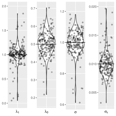
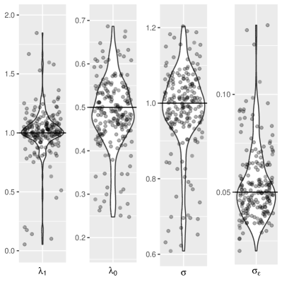
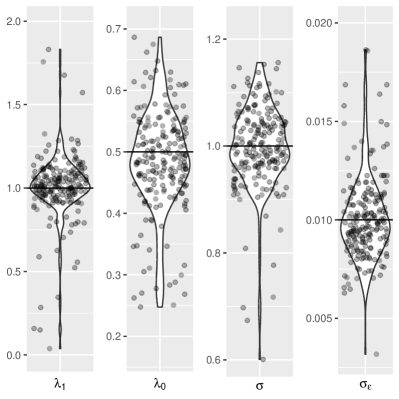
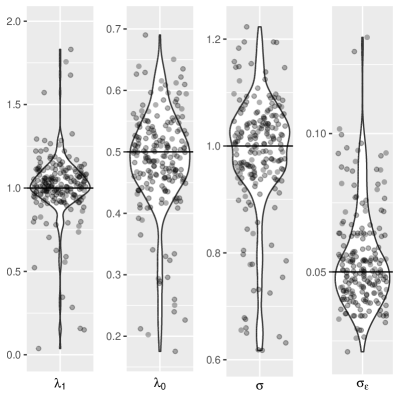
Figure 2. Violin plots of the MCLE in Study 1 with two-piece method (top) and marginal method (bottom) from 200 replicates. The horizontal bar in each panel is the true parameter value $\lambda_{1}=1$, $\lambda_{0}=0.5$, $\sigma=1$, and $\sigma_{\epsilon}=0.01$ (left) and $0.05$ (right). The number of replications is 200.

Figure 2 presents the violin plots of the MCLE in Study 1 of the 200 replicates in comparison to the true values of the four parameters. Violin plots are similar to box plots with a rotated kernel density plot on each side. The horizontal bars in the panels are the true parameter values. For each parameter, the true value lies in the bulk part of the violin plot. This indicates that the true parameters are recovered well by both MCLE methods. The left and right panels represent different sized additional measurement errors. The variation of the estimates in the case of $\sigma_{\epsilon}=0.01$ is smaller than that in the case of $\sigma_{\epsilon}=0.05$, which is expected.

The second simulation study addresses the problem of estimating of standard errors for both MCLE procedures via parametric bootstrap. The sampling horizon (the length of observation window) was set to two levels, 200 and 500 time units. The sampling intervals (the inverse sampling frequency) also had two levels, 1 and 5 time units. The parameters of MRME process were: $\lambda_{1}=1$, $\lambda_{0}=0.5$, $\sigma=1$, and $\sigma_{\epsilon}=0.01$. Table 2 (upper block) summarizes the results. Once again we can see that both the marginal method and the two-piece method recover the true parameters well. Their empirical standard errors are similar, suggesting that the two methods have comparable efficiency for these setups. Moreover, the standard errors were estimated by the parametric bootstrap procedure with 50 replications. The estimated standard errors are reasonably close to empirical ones. The coverage rates of the 95% bootstrap confidence intervals are as low as 81% for $\lambda_{1}$ for the case with sampling interval 5 and sampling horizon 200. As the sampling interval decreases and the sampling horizon increases, the coverage rates get reasonably close to the nominal level.

Let us make a few remarks on the influence of sampling horizon and sampling interval on the efficiency of estimation. When the sampling interval is held fixed but the sampling horizon is 2.5 times longer, the ESE (empirical standard error) seems to be $\sqrt{2.5}(=1.58)$ times smaller for most parameter estimates. The longer sampling horizon covers more moving-resting cycles ($M_{j}+R_{j}$), and provides more information on both mobility and measurement error parameters. If we fix the sampling horizon and increase sampling frequency by reducing the sampling interval, however, the ESE of only $\hat{\sigma}$ reduces in proportion to the square root of the number of observations. Theoretically, if one can take observations nearly continuously, the mobility parameter $\sigma$ can be estimated with absolute accuracy. Increasing sampling frequency also improves the estimation of $\lambda$s to a certain degree, but improves the estimation of $\sigma_{\epsilon}$ drastically. The results show the difference between the domain expansion asymptotics and the in-fill asymptotics.

Table 2. Summaries of Studies 2 and 3: average estimator (EST), empirical standard error (ESE), average parametric bootstrap standard error (ASE), and coverage rate (CR) of $95\%$ large-sample confidence interval of MCLE with the two-piece method and the marginal method. The number of replications is 200.

Sampling	Sampling	Parameter	True	Two-piece method				Marginal method
horizon	interval		value	EST	ESE	ASE	CR	EST	ESE	ASE	CR
Study 2
200	5	$\lambda_{1}$	1.0	0.961	0.546	0.508	0.80	0.982	0.570	0.516	0.81
		$\lambda_{0}$	0.5	0.493	0.169	0.240	0.93	0.485	0.211	0.251	0.89
		$\sigma$	1.0	0.966	0.189	0.163	0.80	0.970	0.194	0.166	0.82
		$\sigma_{\epsilon}(\times 10^{-2})$	1.0	1.145	0.710	0.651	0.91	1.136	0.665	0.648	0.92
	1	$\lambda_{1}$	1.0	1.104	0.394	0.386	0.94	1.057	0.410	0.414	0.88
		$\lambda_{0}$	0.5	0.502	0.093	0.092	0.96	0.488	0.109	0.109	0.92
		$\sigma$	1.0	1.011	0.084	0.088	0.93	1.001	0.089	0.097	0.92
		$\sigma_{\epsilon}(\times 10^{-2})$	1.0	1.002	0.070	0.068	0.94	1.002	0.069	0.068	0.93
500	5	$\lambda_{1}$	1.0	1.020	0.362	0.342	0.92	1.009	0.354	0.335	0.91
		$\lambda_{0}$	0.5	0.512	0.101	0.111	0.95	0.509	0.106	0.115	0.95
		$\sigma$	1.0	0.982	0.122	0.114	0.91	0.978	0.119	0.112	0.92
		$\sigma_{\epsilon}(\times 10^{-2})$	1.0	1.046	0.356	0.376	0.92	1.045	0.362	0.357	0.90
	1	$\lambda_{1}$	1.0	1.036	0.240	0.224	0.93	0.983	0.224	0.223	0.88
		$\lambda_{0}$	0.5	0.508	0.060	0.058	0.96	0.495	0.064	0.062	0.92
		$\sigma$	1.0	1.008	0.060	0.055	0.92	0.997	0.067	0.058	0.90
		$\sigma_{\epsilon}(\times 10^{-2})$	1.0	0.998	0.044	0.042	0.94	0.998	0.044	0.042	0.93
Study 3
160	0.8	$\lambda_{1}$	1.0	1.139	0.440			1.069	0.549
		$\lambda_{0}$	0.1	0.106	0.030			0.096	0.039
		$\sigma$	1.0	1.013	0.119			0.991	0.140
		$\sigma_{\epsilon}(\times 10^{-2})$	1.0	0.998	0.045			0.998	0.045
200	0.1	$\lambda_{1}$	1.0	1.031	0.238			1.132	0.329
		$\lambda_{0}$	0.1	0.102	0.024			0.109	0.026
		$\sigma$	1.0	1.002	0.040			1.007	0.043
		$\sigma_{\epsilon}(\times 10^{-2})$	1.0	0.999	0.015			0.999	0.015

Finally, let us note that the performance of the two methods is similar in both simulation studies described above. That was surprising because the marginal method basically ignores the dependence of the MRME process and treats increments as if they are independent. One possible explanation is that when the distance between two consecutive observation is relatively long, then the dependence between two consecutive increments of the MRME process is weaker. To illustrate this point, one can calculate the correlation of absolute values of consecutive increments via simulation by employing the auto-correlation function with lag 1 (ACF(1)) and lag 2 (ACF(2)). For example, for the same parameter set as in the above simulations and a long time horizon 100,000, both ACF(1) and ACF(2) for the sampling interval 5 are very close to 0 from a Monte Carlo study. For the sampling interval 0.1, however, they are 0.46 and 0.40, respectively. Our third simulation study was based on this design. We also considered sampling interval 0.8 in the simulation because it has a relatively large ACF(1), 0.23, and a significantly smaller ACF(2), 0.07. The results of Study 3 with these small sampling intervals are presented in Table 2 (lower block). It is clear that the two-piece procedure is preferable for datasets with shorter sampling intervals (more frequent observations).

6. Movement of a Mountain Lion

The MRME model was applied to GPS data collected on a mature female mountain lion living in the Gros Ventre Mountain Range near Jackson, Wyoming. The data were collected by a code-only GPS wildlife tracking collar from 2009 to 2012. The collar was programmed to record locations every 8 hours, but the actual sampling intervals were irregular. In the Grand Teton and Gros Ventre mountains of Wyoming, deep winter snows ensure that mountain-lion movements differ across seasons (Elbroch et al., 2013). So, we fitted a MRME model to the summer data (from June 1, 2012 to August 31, 2012) and winter data (from December 1, 2011 to February 29, 2012), respectively. These two periods of data were plotted as Figure 3. The summer data had an average sampling interval of 5.46 hours with standard deviation 5.14 hours, ranging from 0.5 hours to 32 hours. The average sampling interval was 5.58 hours in the winter data, with standard deviation 4.09 hours and range from 0.5 hours to 25 hours. The summer data has 401 observations and winter data has 392 observations.

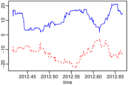
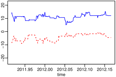
Figure 3. Actual coordinates of a female mountain lion in the Gros Ventre mountain range, Wyoming. The $x$-axis is time in years. The $y$-axis is departure from the starting point. The solid blue line is UTM easting (km) and the dashed red line is UTM northing (km). Left: Summer period data, from June 1, 2012 to August 31, 2012. Right: Winter period data, from December 1, 2011 to February 29, 2012.

The estimates based on two-piece composite likelihood for summer data are $\hat{\lambda}_{1}=2.841$ $\text{hour}^{-1}$, $\hat{\lambda}_{0}=0.179$ $\text{hour}^{-1}$, $\hat{\sigma}=1.335$ $\text{km}/\text{hour}^{1/2}$ and $\hat{\sigma_{\epsilon}}=0.019$ km. On average, this lion was moving 0.352 hours for each 5.587 hours resting, and, if she kept moving for (exactly) one full hour, the average deviation from the initial position is $1.335$ km in both directions (northing and easting). Compared to the summer data, the estimates for winter data are $\hat{\lambda}_{1}=6.225$ $\text{hour}^{-1}$, $\hat{\lambda}_{0}=0.118$ $\text{hour}^{-1}$, $\hat{\sigma}=1.506$ $\text{km}/\text{hour}^{1/2}$ and $\hat{\sigma_{\epsilon}}=0.009$ km, so, during the winter period, she spent $51.7\%$ more time staying in place and $54.4\%$ less time moving. The estimate of $\sigma_{\epsilon}$ (standard deviation of Gaussian noise) indicates that the GPS tracking collar had about 10- to 20-meters of measurement error, and the error is twice as high in summer than in winter, which is consistent with the report by Owari et al. (2009). However, the variability observed by Owari et al. (2009) was primarily due to sky obstruction from broadleaf tree canopy, which cannot be the case for the conifer-dominated mountains in Wyoming. Instead, these differences in GPS error likely reflect the fact that mountain lions in the study area select thicker vegetation with shade and cover in which to bed in the summer and more open terrain with southern aspects in rugged terrain, which catch sun and provide thermoregulatory benefits in the winter (Kusler et al., 2017). The results from the marginal method are similar (Table 3) except that the estimate of the rate parameter $\lambda_{1}$ of the moving state is noticeably smaller. Based on the comparison between the two methods in the simulation study, our discussion used the results from the two-piece method.

Table 3. Analysis results for mountain lion movement data. Point estimates (EST) from both two-piece method and marginal method are reported. Standard error of point estimates are evaluated by parametric bootstrap (SE).

Season	Parameter	Two-piece method		Marginal method
		EST	SE	EST	SE
Summer	$\lambda_{1}$	2.841	0.459	1.090	0.280
	$\lambda_{0}$	0.179	0.014	0.158	0.015
	$\sigma$	1.335	0.106	0.999	0.104
	$\sigma_{\epsilon}(\times 10^{-2})$	1.854	0.087	1.879	0.078
Winter	$\lambda_{1}$	6.225	0.825	4.720	0.711
	$\lambda_{0}$	0.118	0.010	0.114	0.009
	$\sigma$	1.506	0.095	1.454	0.089
	$\sigma_{\epsilon}(\times 10^{-2})$	0.908	0.036	0.934	0.043

7. Discussion

Inactive periods and measurement errors are both necessary features of animal movement models, if we are to successfully reconstruct natural behaviors. Handling measurement errors in the MR process is especially critical because, if discarded, a microscopic amount of measurement error causes substantial bias in estimation. Our approach employing composite likelihood is the first to make the MRME model practically feasible. For movement data from predators that are known to have long inactive periods (Jeschke, 2007), the MRME model has great potential in revealing insights for animal ecologists. For example, the clear seasonal patterns in movement patterns have immediate implications for diverse ecological questions (e.g., seasonal foraging ecology, Elbroch et al., 2013) and estimating animal abundance using models dependent upon animal speed (Moeller et al., 2018).

The MRME model can be extended to meet further practical needs. For some predators, an inactive period may have different purposes, such as resting and food handling. Pozdnyakov et al. (2020) introduced the moving-resting-handling (MRH) process that allows two different types of motionless states. The moving period may also represent different behaviors (Benhamou, 2011; Kranstauber et al., 2012), and this can be accommodated by allowing the volatility parameter to have multiple levels. More generally, animal behavior depends on a suite of intrinsic and extrinsic variables. Our MRME model provides an important benchmark for building these more realistic extensions.

Appendix A Formulas for High Dimensions

Let ${\mathbf{X}}(t_{k})$ and ${\mathbf{Z}}(t_{k})$ be $d$-dimensional random vectors. Set ${\mathbf{X}}(t_{k})=(X_{1}(t_{k}),\dots,X_{d}(t_{k}))$, $\mathbf{\epsilon_{k}}=(\epsilon_{1k},\dots,\epsilon_{dk})\sim\mathrm{MN}(\mathbf{0},\sigma_{\epsilon}^{2}\mathbf{I})$, and $\mathbf{\epsilon_{i}}$ and $\mathbf{\epsilon_{j}}$ are independent for $i\neq j$. Then, ${\mathbf{Z}}(t_{k})=(Z_{1}(t_{k}),\dots,Z_{d}(t_{k}))=(X_{1}(t_{k})+\epsilon_{1k},\dots,X_{d}(t_{k})+\epsilon_{dk})$. The density $h_{ij}$ in the $d$-dimension case is given by

$$h_{10}({\mathbf{x}},t)=\int_{0}^{t}\prod_{i=1}^{d}\phi(x_{i};\sigma^{2}w)p_{10}(w,t)\mathrm{d}w.$$

Then we get that

$$g_{10}({\mathbf{z}},t) =\int_{\mathbb{R}}\dots\int_{\mathbb{R}}h_{10}({\mathbf{z}}-{\mathbf{x}};\sigma^{2}w)\prod_{i=1}^{d}\phi(x_{i};2\sigma_{\epsilon}^{2})\mathrm{d}x_{1}\dots\mathrm{d}x_{d}$$

$$=\int_{\mathbb{R}}\dots\int_{\mathbb{R}}\left[\int_{0}^{t}\prod_{i=1}^{d}\phi(z_{i}-x_{i};\sigma^{2}w)p_{10}(w,t)\mathrm{d}w\right]\prod_{i=1}^{d}\phi(x_{i};2\sigma_{\epsilon}^{2})\mathrm{d}x_{1}\dots\mathrm{d}x_{d}$$

$$=\int_{0}^{t}\prod_{i=1}^{d}\left[\int_{\mathbb{R}}\phi(z_{i}-x_{i};\sigma^{2}w)\phi(x_{i};2\sigma_{\epsilon}^{2})\mathrm{d}x_{i}\right]p_{10}(w,t)\mathrm{d}w.$$

Similarly, we also have

$$g_{00}({\mathbf{z}},t)= \int_{0}^{t}\prod_{i=1}^{d}\left[\int_{\mathbb{R}}\phi(z_{i}-x_{i};\sigma^{2}(t-w))\phi(x_{i};2\sigma_{\epsilon}^{2})\mathrm{d}x_{i}\right]p_{00}(w,t)\mathrm{d}w+e^{-\lambda_{0}t}\prod_{i=1}^{d}\phi(z_{i},2\sigma_{\epsilon}^{2}),$$

$$g_{01}({\mathbf{z}},t)= \int_{0}^{t}\prod_{i=1}^{d}\left[\int_{\mathbb{R}}\phi(z_{i}-x_{i};\sigma^{2}(t-w))\phi(x_{i};2\sigma_{\epsilon}^{2})\mathrm{d}x_{i}\right]p_{01}(w,t)\mathrm{d}w,$$

$$g_{11}({\mathbf{z}},t)= \int_{0}^{t}\prod_{i=1}^{d}\left[\int_{\mathbb{R}}\phi(z_{i}-x_{i};\sigma^{2}w)\phi(x_{i};2\sigma_{\epsilon}^{2})\mathrm{d}x_{i}\right]p_{11}(w,t)\mathrm{d}w$$

$$+e^{-\lambda_{1}t}\prod_{i=1}^{d}\left[\int_{\mathbb{R}}\phi(z_{i}-x_{i};\sigma^{2}t)\phi(x_{i};2\sigma_{\epsilon}^{2})\mathrm{d}x_{i}\right].$$

Let us mention that these formulas do not require numerical multiple integral evaluation and, as a consequence, are computationally efficient.

References

- Andrieu et al. (2010) C. Andrieu, A. Doucet and R. Holenstein (2010). “Particle Markov chain Monte Carlo methods.” Journal of the Royal Statistical Society: Series B (Statistical Methodology) 72, 269–342.
- Benhamou (2011) S. Benhamou (2011). “Dynamic approach to space and habitat use based on biased random bridges.” PLoS ONE 6, e14592.
- Brett et al. (2012) T. M. Brett, K. Ruth, T. Len, M. Jason, J. M. Bernie and M. M. Juan (2012). “A general discrete-time modeling framework for animal movement using multistate random walks.” Ecological Monograph 82, 335–349.
- Brillinger (2010) D. R. Brillinger (2010). “Modeling spatial trajectories.” In A. E. Gelfand, P. J. Diggle, M. Fuentes and P. Guttorp (eds.), Handbook of Spatial Statistics, pp. 463–476. Chapman & Hall/CRC Boca Raton, Florida, USA.
- Cagnacci et al. (2010) F. Cagnacci, L. Boitani, R. A. Powell and M. S. Boyce (2010). “Animal ecology meets GPS-based radiotelemetry: A perfect storm of opportunities and challenges.” Philosophical Transactions of the Royal Society B: Biological Sciences 365, 2157–2162.
- Cappé et al. (2005) O. Cappé, E. Moulines and T. Rydén (2005). Inference in Hidden Markov Models. Springer.
- Elbroch et al. (2013) L. M. Elbroch, P. E. Lendrum, J. Newby, H. Quigley and D. Craighead (2013). “Seasonal foraging ecology of non-migratory cougars in a system with migrating prey.” PLOS ONE 8, e83375.
- Godambe (1960) V. P. Godambe (1960). “An optimum property of regular maximum likelihood estimation.” Ann. Math. Statist. 31, 1208–1211.
- Hooten et al. (2017) M. B. Hooten, D. S. Johnson, B. T. McClintock and J. M. Morales (2017). Animal Movement: Statistical Models for Telemetry Data. CRC Press.
- Horne et al. (2007) J. S. Horne, E. O. Garton, S. M. Krone and S. Lewis, J (2007). “Analyzing animal movements using Brownian bridges.” Ecology 88, 2354–2363.
- Hu et al. (2020a) C. Hu, V. Pozdnyakov and J. Yan (2020a). “Density and distribution evaluation for convolution of independent gamma variables.” Computational Statistics 35, 327–342.
- Hu et al. (2020b) C. Hu, V. Pozdnyakov and J. Yan (2020b). smam: Statistical Modeling of Animal Movements. R package version 0.4.0.9000. (GitHub: https://github.com/ChaoranHu/smam).
- Ionides et al. (2011) E. L. Ionides, A. Bhadra, Y. Atchadé and A. King (2011). “Iterated filtering.” The Annals of Statistics 39, 1776–1802.
- Ionides et al. (2015) E. L. Ionides, D. Nguyen, Y. Atchadé, S. Stoev and A. A. King (2015). “Inference for dynamic and latent variable models via iterated, perturbed Bayes maps.” Proceedings of the National Academy of Sciences 112, 719–724.
- Jeschke (2007) J. M. Jeschke (2007). “When carnivores are “full and lazy”.” Oecologia 152, 357–364.
- Jonsen et al. (2005) I. D. Jonsen, J. M. Flemming and R. A. Myers (2005). “Robust state-space modeling of animal movement data.” Ecology 86, 2874–2880.
- King et al. (2016) A. A. King, D. Nguyen and E. L. Ionides (2016). “Statistical inference for partially observed Markov processes via the R package pomp.” Journal of Statistical Software 69, 1–43.
- Kranstauber et al. (2012) B. Kranstauber, R. Kays, S. D. LaPoint, M. Wikelski and K. Safi (2012). “A dynamic Brownian bridge movement model to estimate utilization distributions for heterogeneous animal movement.” Journal of Animal Ecology 81, 738–746.
- Kusler et al. (2017) A. Kusler, L. M. Elbroch, H. Quigley and M. Grigione (2017). “Bed site selection by a subordinate predator: an example with the cougar (Puma concolor) in the greater yellowstone ecosystem.” PeerJ 5, e4010.
- Lindsay (1988) B. G. Lindsay (1988). “Composite likelihood methods.” Contemporary Mathematics 80, 221–239.
- Mashanova et al. (2010) A. Mashanova, T. H. Oliver and V. A. Jansen (2010). “Evidence for intermittency and a truncated power law from highly resolved aphid movement data.” Journal of The Royal Society Interface 7, 199–208.
- Moeller et al. (2018) A. K. Moeller, P. M. Lukacs and J. S. Horne (2018). “Three novel methods to estimate abundance of unmarked animals using remote cameras.” Ecosphere 9, e02331.
- Nelder and Mead (1965) J. A. Nelder and R. Mead (1965). “A simplex method for function minimization.” The Computer Journal 7, 308–313.
- Owari et al. (2009) T. Owari, H. Kasahara, N. Oikawa and S. Fukuoka (2009). “Seasonal variation of global positioning system (GPS) accuracy within the tokyo university forest in hokkaido.” Bulletin of Tokyo University Forests 120, 19–28.
- Patterson et al. (2008) T. Patterson, L. Thomas, C. Wilcox, O. Ovaskainen and J. Matthiopoulos (2008). “State-space models of individual animal movement.” Trends in Ecology and Evolution 23, 87–94.
- Patterson et al. (2017) T. A. Patterson, A. Parton, R. Langrock, P. G. Blackwell, L. Thomas and R. King (2017). “Statistical modelling of individual animal movement: An overview of key methods and a discussion of practical challenges.” AStA Advances in Statistical Analysis 101, 399–438.
- Pozdnyakov et al. (2019) V. Pozdnyakov, L. Elbroch, A. Labarga, T. Meyer and J. Yan (2019). “Discretely observed Brownian motion governed by telegraph process: Estimation.” Methodology and Computing in Applied Probability 21, 907–920.
- Pozdnyakov et al. (2020) V. Pozdnyakov, L. M. Elbroch, C. Hu, T. Meyer and J. Yan (2020). “On estimation for Brownian motion governed by telegraph process with multiple off states.” Methodology and Computing in Applied Probability .
- Pozdnyakov et al. (2014) V. Pozdnyakov, T. H. Meyer, Y.-B. Wang and J. Yan (2014). “On modeling animal movements using Brownian motion with measurement error.” Ecology 95, 247–253.
- Preisler et al. (2004) H. K. Preisler, A. A. Ager, B. K. Johnson and J. G. Kie (2004). “Modeling animal movements using stochastic differential equations.” Environmetrics 15, 643–657.
- Ueno et al. (2012) T. Ueno, N. Masuda, S. Kume and K. Kume (2012). “Dopamine modulates the rest period length without perturbation of its power law distribution in Drosophila melanogaster.” PLoS One 7, e32007.
- Varin et al. (2011) C. Varin, N. Reid and D. Firth (2011). “An overview of composite likelihood methods.” Statistica Sinica 21, 5–42.
- Yan et al. (2014) J. Yan, Y.-W. Chen, K. Lawrence-Apfel, I. Ortega, V. Pozdnyakov, S. Williams and T. Meyer (2014). “A moving-resting process with an embedded Brownian motion for animal movements.” Population Ecology 56, 401–415.
- Zacks (2004) S. Zacks (2004). “Generalized integrated telegraph processes and the distribution of related stopping times.” Journal of Applied Probability 41, 497–507.