In-situ adaptive reduction of nonlinear multiscale structural dynamics models

Abstract

Conventional offline training of reduced-order bases in a predetermined region of a parameter space leads to parametric reduced-order models that are vulnerable to extrapolation. This vulnerability manifests itself whenever a queried parameter point lies in an unexplored region of the parameter space. This paper addresses this issue by presenting an in-situ, adaptive framework for nonlinear model reduction where computations are performed by default online, and shifted offline as needed. The framework is based on the concept of a database of local Reduced-Order Bases (ROBs), where locality is defined in the parameter space of interest. It achieves accuracy by updating on-the-fly a pre-computed ROB, and approximating the solution of a dynamical system along its trajectory using a sequence of most-appropriate local ROBs. It achieves efficiency by managing the dimension of a local ROB, and incorporating hyperreduction in the process. While sufficiently comprehensive, the framework is described in the context of dynamic multiscale computations in solid mechanics. In this context, even in a nonparametric setting of the macroscale problem and when all offline, online, and adaptation overhead costs are accounted for, the proposed computational framework can accelerate a single three-dimensional, nonlinear, multiscale computation by an order of magnitude, without compromising accuracy.

1 Introduction

Heterogeneous materials are encountered to an increasing extent in simulation-based engineering applications involving structural analysis of solids. Applications include, but are not limited to, advanced modular armor protection [1], design of new materials with special-purpose optimized properties [2], and bone fracture risk assessment [3]. When the scale of the heterogeneity is such that multiple disparate spatial scales require resolution in order to achieve a reliable prediction, multiscale homogenization can be a viable alternative to prohibitively expensive direct numerical simulation involving a massive monolithic discretization [4].

In principle, the method of multiscale homogenization assumes that the material configuration is homogeneous at the macroscale level, but heterogeneous at the level of the smallest represented scale. The evaluation of a conventional constitutive response function at each macroscale material point is replaced by the solution of a discrete Boundary Value Problem (BVP) whose computational domain is a so-called microscale Representative Volume Element (RVE) characterizing the microstructure. The complete BVP is formulated with prescribed boundary deformations corresponding to the deformation gradient at the macroscale material point. The sequence of scales is coupled by formalized procedures of localization and homogenization to transmit information between differing scales [5, 6, 7, 8]. In this work, a particular variant of the method of multiscale homogenization known as “Finite Element squared” or FE² is considered as a starting point. As the name implies, in this variant the Finite Element (FE) method is used to discretize both the macroscopic computational domain and the microscale RVE. The repeated solution of the FE BVP at each material point is an acknowledged computational bottleneck, motivating the development of alternative surrogate models to accelerate this task. Projection-based Model Order Reduction (PMOR) equipped with a second-tier hyperreduction approximation is one established technique for reducing the computational complexity of nonlinear FE models that has recently been demonstrated to be an effective candidate surrogate model in the context of multiscale homogenization [9]. Alternative surrogate model candidates include regression-based models constructed using various methods including Kriging and artificial neural networks. Such methods can potentially lead to more computationally efficient surrogate model evaluation compared to PMOR; however a large amount of data may be required to train the model when the constitutive response is complex. To accelerate the acquisition of training data, PMOR again presents a useful computational technology. In this work, a multifidelity framework leveraging low-, medium- and high-fidelity models is proposed to achieve a computationally tractable end-to-end procedure for nonlinear multiscale simulations. The proposed framework features a novel in-situ construction and utilization of an adaptive PMOR to eliminate computation bottlenecks. The usefulness of this novelty is not restricted to the current application of interest (i.e. multiscale modeling); benefits are anticipated in other related processes such as multifidelity optimization. It is therefore presented in what follows as a general-purpose methodology.

PMOR is typically embedded in an offline-online computational framework. In the phase of non-time-critical, offline training, information data from a High Dimensional Model (HDM) are collected and used to construct a Reduced-Order Basis (ROB) – for example, using Proper Orthogonal Decomposition (POD) and the method of snapshots [10] – and the corresponding Projection-based Reduced Order Model (PROM). Then, in the phase of time-critical, online evaluation, an approximate solution is computed using the PROM as a surrogate model for the underlying HDM. This offline-online decomposition of the computational effort is appropriate in real-time applications that are performed for the exploration of a space of interest associated with some usually but not necessarily physical model parameters, such as in design optimization [11, 12], uncertainty quantification [13, 14], and repeated analysis [15, 16]. In these cases where the space of one or more physical macroscopic parameters (such as those defining the geometry, boundary/initial conditions, or material properties) is explored, the offline cost is amortized by the sizable number of required analyses associated with the number of parameter points necessary to adequately perform this exploration. Consequently, the overall speedup can still be significant even when the potentially substantial offline cost is accounted for. Here, it is emphasized that in the context of multiscale homogenization, PMOR is computationally feasible even in the nonparametric setting due to the large number of microscale RVE simulations that are required at a single macroscopic parameter point. Hence, a desirable speedup of the multiscale computations can be still achieved by building PROMs for all smaller scales. Furthermore, a nonparametric application calls for an in-situ alternative to the conventional offline-online strategy, where the construction and utilization of the hyperreduced PROM (HPROM) can be performed during the multiscale simulation without requiring any preliminary computational work, using solution snapshots collected during already performed microscale RVE computations.

Several existing PMOR methods have been previously developed and applied to the solution of nonlinear multiscale problems. In [17], a PROM of the microscale problem was constructed based on an á priori training strategy that involved computing solution snapshots using predefined microstrain histories. This approach was subsequently extended in [18] to formulations with periodic boundary conditions for the microscale model. However, in each of these works the PROMs were not equipped with a hyperreduction method and consequently the resulting speedup factor was limited to about an order of magnitude, even without accounting for the offline costs. More recently, the co-authors of [9] introduced a nonlinear PMOR framework incorporating the Energy Conserving Sampling and Weighting (ECSW) hyperreduction method [19, 20] which significantly reduced the computational cost of multiscale problems characterized by large deformations and material nonlinearity, including when the offline costs were taking into account. Specifically, the computational framework proposed in [9] included a two-step training strategy where: a microscale HPROM is first constructed in-situ in order to achieve significant speedups even in nonparametric settings; next, a conventional offline-online training approach is performed to build a parametric macroscale HPROM. A notable feature of this approach is the reduction in the cost of the training by using the in-situ microscale HPROM to accelerate macroscale snapshot acquisition. However, a weakness of the proposed framework is its vulnerability to extrapolation if the underlying approximation subspace is not sufficiently explored during the in-situ training phase.

The alternative in-situ training strategy proposed in this paper avoids extrapolation by incorporating an adaptive HPROM construction based on the concept of a database of local Reduced-Order Bases (ROBs) constructed and updated on-the-fly. This process treats the components of the deformation gradient as a parameter vector, which facilitates the locating of each microscale BVP within the database in order to assign to it online the most-appropriate local ROB. Accuracy is optimized by collecting new snapshots and other additional information as needed and updating accordingly the local ROBs. This usage of local ROBs enables the efficient solution of difficult problems for which PMOR is not effectively performed by constructing a single global ROB. Note that locality in this paper refers to the parameter space characterized by the deformation gradient, in sharp contrast with previous works where locality was considered with respect to the solution manifold [21].

The remainder of this paper is organized as follows. Section 2 provides a brief summary of the FE² multiscale homogenization method. Section 3 introduces the microscale HPROM and its training strategy. This section also highlights the necessity for ROB adaptation to avoid extrapolation. Section 4 proposes a novel, online, in-situ ROB adaptation approach suitable for nonlinear, multifidelity, multiscale, computational homogenization. Section 5 provides an assessment of the overall proposed adaptive PMOR framework using several representative applications, and demonstrates its ability to deliver speedups while compromising neither stability nor accuracy.

2 The FE² computational framework

In this section a brief summary of the FE² method is provided, focusing on the aspects that are relevant to subsequent developments including notation. For a comprehensive formulation of multiscale homogenization, the interested reader is referred to [9] and the references cited therein. The fundamental generalization underlying FE² is that the evaluation of stress as a function of strain for a heterogeneous material is governed by the solution of a locally attached boundary value problem characterizing its microstructure. This concept can be applied recursively to materials that exhibit $n_{s}+1$ separated scales; in what follows $k=0,\ldots,n_{s}$ denotes the sequence of scales (or levels), with $k=0$ and $k=1,\ldots,n_{s}$ designating the macroscale and the finer meso/microscales, respectively. Specifically, at the $n_{s}$ coarsest scales ($k=0,\ldots,n_{s}-1$) each stress-strain relation is associated with a locally attached microstructure, while at the finest scale ($k=n_{s}$) the stress-strain relation is defined by a conventional constitutive law.

2.1 Semi-discrete governing equations

In this work, a distinction is made between constrained and unconstrained Degrees Of Freedom (DOFs), the former being those whose values are specified by essential boundary conditions, while the latter are subject to no such restriction. Following the notation of [9], $\stackrel{{\scriptstyle\circ}}{{\bm{v}}}_{k}$ is defined here as a vector over the set of constrained DOFs at level $k$, $\bm{v}_{k}$ as the corresponding vector over the set of unconstrained DOFs at level $k$, and $\overline{\bm{v}}_{k}$ as the concatenation of these two vectors. A similar notation is adopted for matrices. It follows that a subscript $0$ attached to any vector or matrix designates a macroscopic quantity. Using this notation and assuming that $\ddot{\stackrel{{\scriptstyle\circ}}{{\bm{u}}}}_{0}=0$, the semi-discrete form of the equations of motion governing dynamic equilibrium can be written as

$$\bm{M}_{0}\ddot{\bm{u}}_{0}+\bm{f}_{0}\left(\bm{u}_{0},\stackrel{{\scriptstyle\circ}}{{\bm{u}}}_{0},\bm{\xi}_{0}\right) =\bm{0}$$ (1)

$$\bm{f}_{k}\left(\bm{u}_{k},\stackrel{{\scriptstyle\circ}}{{\bm{u}}}_{k},\bm{\xi}_{k}\right) =\bm{0}$$

for $k=1,\ldots,n_{s}$, where $\bm{M}$ is a FE mass matrix, $\bm{f}$ is a FE vector of internal forces, $\bm{u}$ and $\ddot{\bm{u}}$ are FE vectors of displacements and accelerations, respectively, and $\bm{\xi}$ is a vector of history variables associated with certain constitutive laws such as elastoplasticity when introduced at the level $k=n_{s}$. For levels $0\leq k<n_{s}$, $\bm{\xi}_{k}$ consists of the set of history variables at all material points of the attached microstructure. The governing equations (1) are coupled by the localization and homogenization conditions presented in the next section.

2.2 Scale transmission conditions

Kinematic information is transmitted from coarser to finer scales via prescribed nonhomogeneous displacement boundary conditions applied to the exterior boundary of the attached microstructure. These prescribed values are specified such that the volumetric average of the deformation gradient at the finer scale is identical to the deformation gradient at the material point of the coarser scale to which the microstructure is attached. This is referred to as the localization condition and can be expressed as follows

$$\stackrel{{\scriptstyle\circ}}{{\bm{U}}}_{k+1}=\stackrel{{\scriptstyle\circ}}{{\bm{X}}}_{k+1}\left(\bm{F}_{k}-\bm{I}\right)$$ (2)

where $\bm{F}_{k}$ is the coarse-scale deformation gradient, $\bm{I}$ is the $3\times 3$ identity matrix, and $\stackrel{{\scriptstyle\circ}}{{\bm{U}}}_{k+1}$ is the matrix whose three columns contain the prescribed $x$-, $y$- and $z$-components of displacement. In other words, the displacement vector over the set of constrained DOFs at level $k+1$, $\stackrel{{\scriptstyle\circ}}{{\bm{u}}}_{k+1}$, is obtained – up to a permutation – by stacking the columns of $\stackrel{{\scriptstyle\circ}}{{\bm{U}}}_{k+1}$. Similarly, $\stackrel{{\scriptstyle\circ}}{{\bm{X}}}_{k+1}$ is the matrix whose three columns contain the $x$-, $y$- and $z$-coordinates in the reference configuration of the nodes on the exterior boundary of the attached microstructure whose DOFs are constrained. In the particular case of the so-called uniform essential boundary conditions, the values of all DOFs located on the exterior boundary of the attached microstructure are prescribed. Alternatively, in the case of periodic boundary conditions, only a minimal set of corner points have prescribed displacements while the remaining exterior boundary DOFs are constrained using linear multipoint constraint equations to enforce the periodicity of the fluctuations between each pair of opposite faces.

After computing the response of an attached microstructure to the prescribed boundary displacements, information is transmitted back from finer to coarser scales in the form of a homogenized stress tensor defined as the volumetric average of the stress in the attached microstructure. This quantity can be conveniently obtained from the reaction forces associated with the constrained boundary DOFs as follows

$$\bm{P}_{k}=\frac{1}{\left|\mathcal{B}_{k+1}\right|}\bm{X}_{k+1}^{T}\stackrel{{\scriptstyle\circ}}{{\bm{R}}}_{k+1}$$

where $\bm{P}_{k}$ is the coarse-scale homogenized first Piola-Kirchhoff stress tensor, $\left|\mathcal{B}_{k+1}\right|$ is the volume of the RVE, and $\stackrel{{\scriptstyle\circ}}{{\bm{R}}}_{k+1}$ is the matrix whose three columns contain the $x$-, $y$-, and $z$-components of the internal force vector of the nodes on the exterior boundary of the attached microstructure whose DOFs are constrained, i.e. the boundary reaction forces.

In summary, the multiscale computational model distinguishes itself from a conventional FE model in that it involves repeatedly solving one or more microscale BVPs, with one such solution required for each stress-strain evaluation at all scales other than the finest. For a given RVE, the microscale BVPs vary only in the values of the prescribed boundary displacements. Regardless of whether uniform or periodic boundary conditions are adopted, (2) shows that the computational response of the microscale model can be characterized as an implicit function of nine components of the deformation gradient $\bm{F}_{k-1}$. In Section 4, the set of components of $\bm{F}_{k-1}$ is treated as a parameter vector as in the parametric setting of PMOR. The parameter space $\mathcal{D}_{k}\subset\mathbb{R}^{n_{sd}}$, where $n_{sd}=4$ for two-dimensional problems, $n_{sd}=9$ for three-dimensional ones, and $\bm{F}_{k-1}\in\mathcal{D}_{k}$, is explored by solving the microscale BVP repeatedly in order to generate snapshots of the microstructural response as required for the construction of a surrogate model.

At each computational time-step of a single multiscale simulation, a total of $\prod_{k=0}^{n_{s}-1}\left|\mathcal{G}_{k}\right|$ high-dimensional, microscale BVPs are solved at the finest scale, where $\left|\mathcal{G}_{k}\right|$ denotes the number of Gauss points at level $k$. The overall computational cost associated with such a computational complexity can be prohibitive for large-scale multiscale models, which motivates PMOR to truncate the computational complexity by reducing the operational dimensionality of the multiscale model. Even in the absence of a physical parametric setting at the macroscale level, computational savings are still feasible if the macroscale model is not reduced, but rather a sequence of HPROMs are constructed at all other scales $k$, $k=1,\ldots,n_{s}$. For this setting, the co-authors of [9] proposed an in-situ training strategy for microscale reduction where only the single multiscale simulation of interest is required to be performed, without any predefined offline computational work. This methodology will be described in the following section, after which a novel contribution will be presented to extend the scope and robustness of the in-situ concept without sacrificing its inherent convenience.

3 Projection-based model order reduction

Here, the application of PMOR to the FE² computation framework is reviewed. Specifically, the POD reduction and ECSW hyperreduction methods are used to construct a surrogate model to accelerate the solution of each locally attached microstructural FE model at all fine scales ($k=1,\ldots,n_{s}$). Training is performed in-situ (or on-the-fly), pursuant to our objective of enabling a computational technology for multiscale modeling that is tractable, robust, and convenient for simulators accustomed to conventional materials. Although not considered in what follows, PMOR can also be applied to the macroscale BVP ($k=0$, see [9]).

3.1 Microscale reduction framework

At each fine scale $k$, $k=1,\ldots,n_{s}$, the number of DOFs $n_{k}^{d}$ of the computational FE model is reduced by searching for the solution $\bm{u}_{k}$ of the problem of interest in a low-dimensional subspace – that is,

$$\bm{u}_{k}\approx\bm{V}_{k}\bm{y}_{k}$$ (3)

where $\bm{V}_{k}\in\mathbb{R}^{n_{k}^{d}\times s_{k}}$ is a ROB constructed using POD and the method of snapshots [10], $\bm{y}_{k}\in\mathbb{R}^{s_{k}}$ is a vector of generalized coordinates, and $s_{k}\ll n_{k}^{d}$. The snapshots from which the ROB is constructed correspond to high-dimensional solutions of the microstructural FE model that are collected and processed in-situ. The term in-situ indicates that such solutions are obtained during the same multiscale simulation in which the model reduction framework is utilized, in contrast to online-offline treatments.

The dimensionality of the semi-discrete equations governing the microscale BVP (1) is reduced by performing a Galerkin projection – that is, substituting (3) into these equations and pre-multiplying them by the transpose of $\bm{V}_{k}$. This leads to the microscale PROM

$$\bm{V}_{k}^{T}\bm{f}_{k}\left(\bm{V}_{k}\bm{y}_{k},\stackrel{{\scriptstyle\circ}}{{\bm{u}}}_{k},\bm{\xi}_{k}\right)=\bm{0},\qquad k=1,\ldots,n_{s}$$ (4)

where the superscript $T$ designates the transpose operation.

Furthermore, a second-tier hyperreduction approximation is also introduced to avoid computations that scale with the size $n_{k}^{d}$ of the HDM at each level $k>0$. In this work, the ECSW method [19, 20] is preferred for this purpose due to its structure-preserving property [20] and the simplicity by which its approximation error can be controlled, namely, via a user-specified thresholding parameter. As the name suggests, ECSW samples a subset $\widetilde{\cal E}_{k}$ of the element set ${\cal E}_{k}$ of a given FE mesh – that is, $\widetilde{\cal E}_{k}\subset{\cal E}_{k}$ – and assigns to each sampled element $e$ a positive weight $\alpha_{k}^{e}\geqslant 0$. The internal force term in the microscale PROM (4) is evaluated by simply weighting the contributions of the sampled elements only, i.e.

$$\bm{V}_{k}^{T}\bm{f}_{k}\left(\bm{V}_{k}\bm{y}_{k},\stackrel{{\scriptstyle\circ}}{{\bm{u}}}_{k},\bm{\xi}_{k}\right)\approx\sum_{e\,\in\,{\widetilde{\cal E}}_{k}}\alpha_{k}^{e}\left(\bm{V}_{k}^{e}\right)^{T}\bm{f}_{k}^{e}\left(\bm{V}_{k}^{e}\bm{y}_{k},\stackrel{{\scriptstyle\circ}}{{\bm{u}}}_{k}^{e},\bm{\xi}_{k}^{e}\right)=\bm{f}_{k}^{r}\left(\bm{y}_{k},\stackrel{{\scriptstyle\circ}}{{\bm{u}}}_{k},\bm{\xi}_{k}\right)$$ (5)

In the above expressions, the superscript $e$ designates the restriction of a global vector or matrix to element $e$. The optimal reduced mesh $\widetilde{\cal{E}}_{k}$ and associated weights can be estimated using either the Non-Negative Least Squares (NNLS) algorithm proposed by Lawson and Hanson [22] or alternative sparsity promoting L1-minimization methods [23].

In the context of the microscale reduction framework, reduction and hyperreduction are considered not only for the unconstrained part of the internal force vector as shown in (5), but also for both the constrained part of the internal force required for the homogenization condition and the linear constraint equations required for the enforcement of periodic boundary conditions [9].

3.2 In-situ training strategy

As already stated in Section 2, the deformation gradient $\bm{F}_{k-1}$ at a Gauss point characterizes the microscale BVP at level $k$, $k=1,\ldots,n_{s}$. In what follows, each microscale BVP at level $k$ is associated with a parameter vector $\bm{z}_{k}$ in the parameter space $\mathcal{D}_{k}\subset\mathbb{R}^{sd}$ (also referred to in the remainder of this section as parameter “point” in $\mathcal{D}_{k}$), where $\bm{z}_{k}$ is obtained by stacking the columns of $\bm{F}_{k-1}$. This parametric interpretation of the attached microstructure BVPs motivates the adaptive reduction process discussed in Section 4.

At each computational time-step of a multiscale simulation, $\prod_{j=0}^{k-1}\left|\mathcal{G}_{j}\right|$ microscale BVPs are solved at level $k$, $k=1,\ldots,n_{s}$. This suggests that sufficient training data can be acquired for the purpose of constructing a PROM at each level $k$, $k=1,\ldots,n_{s}$. An in-situ microscale training strategy proposed in [9] that leverages this observation can be described by the following steps:

1. Solve at level $k$, $k=1,\ldots,n_{s}$, a sufficient number $n_{k-1}^{\mathcal{G}}$ of high-dimensional microscale BVPs encountered at the Gauss points of level $k-1$, and sample the resulting solution snapshots (note that $n_{k}^{\mathcal{G}}$ is not necessarily equal to $\left|\mathcal{G}_{k}\right|$).

2. Construct a global ROB $\bm{V}_{k}$.

3. Construct a reduced mesh $\widetilde{\cal{E}}_{k}$.

4. Exploit the resulting HPROM at level $k$ to solve all remaining microscale BVPs at this level.

This nonadaptive, in-situ, microscale training strategy, where the choice for $n_{k-1}^{\mathcal{G}}$ is user-specified (and therefore arbitrary), may encounter scenarios involving extrapolation when the remaining microscale BVPs visit an unexplored region of the parameter space $\mathcal{D}_{k}$. If a queried parameter point falls outside of the subregion defined by the set of sampled points, a good approximate solution of the microscale BVP may not be computable in the existing low-dimensional subspace $\bm{V}_{k}$. However, an adaptive in-situ training strategy has the potential to avoid extrapolation by collecting new high-dimensional solution snapshots and using them to enrich the subspace of approximation when a scenario that would otherwise involve extrapolation is detected.

Typically, the enrichment of the approximation subspace needed when the explored domain within $\mathcal{D}_{k}$ is enlarged requires the expansion of the dimension of the ROB, leading to a deterioration in the attainable speedup. When the dimension of the expanded ROB exceeds a certain threshold, a method is proposed next to split the global ROB into two or more local ROBs, and subsequently find an approximate solution at each queried parameter point using the most suitable of pre-computed and stored local ROBs. A similar approach was proposed in [21] for constructing local ROBs, where locality was defined however with respect to the solution manifold. This approach is not ideally-suited for use with in-situ microscale training as it requires the clustering of solution snapshots, which can be computationally expensive in this context. Thus, this paper proposes an adaptive PMOR strategy with a method of databases containing local ROBs, where locality is defined with respect to the parameter space. The details of this proposal are presented in Section 4.

4 Adaptive in-situ sampling and local reduced-order bases

Next, an in-situ, adaptive sampling process based on the concept of a database $\mathcal{DB}_{k}$ of local ROBs at each level $k$, $k=1,\ldots,n_{s}$, is presented. It leverages the accuracy and computational efficiency of the PMOR framework. The detection of extrapolation when solving a queried microscale BVP is performed using a residual-based error indicator. When an update criterion is triggered by this indicator at level $k$, new information is sampled and used to enrich the content of $\mathcal{DB}_{k}$. In order to preserve the computational efficiency of PMOR, a local ROB is split into two smaller ones if its current size exceeds a certain limit.

In principle, each time a local ROB is updated, the corresponding reduced mesh should also be updated – because the training of ECSW depends on the state of the ROB. Therefore, the HPROM should be updated too accordingly. However, efficiently performing such updates is outside the scope of this paper: it is the subject of ongoing research. With multiple local ROBs stored in a database $\mathcal{DB}_{k}$, the most-appropriate local ROB and associated HPROM must be identified to solve a microscale BVP queried at level $k$.

In order to construct such an adaptive PMOR framework, both the microscale solution snapshots and the underlying deformation gradient parameter points are collected. In order to describe this adaptive framework, the following additional nomenclature and notation are introduced:

• ${\cal S}_{z}^{m_{k}}=\left\{\bm{z}_{k}^{(1)},\ldots,\bm{z}_{k}^{\left(m_{k}\right)}\right\}$, denotes a set of $m_{k}$ deformation gradient parameter points considered among those that have already been sampled at level $k$, and $\bm{z}_{k}^{(i)}\in\mathcal{D}_{k}$, $i=1,\ldots,m_{k}$. It is collected in the matrix

  $$\bm{N}_{k}^{z}=\left[\bm{z}_{k}^{(1)}\cdots\bm{z}_{k}^{\left(m_{k}\right)}\right]\in\mathbb{R}^{{n_{sd}}\times m_{k}}$$

• $\bm{N}_{k}^{u}$ denotes the corresponding snapshot matrix whose $i$-th column stores the HDM-based solution of the microscale BVP characterized by $\bm{z}_{k}^{(i)}$.

4.1 Detection of extrapolation and other large errors

When applied to the solution of a microscale BVP queried at an unsampled parameter point $\bm{z}_{k}^{\star}\in\mathcal{D}_{k}$, a local, in-situ-trained, microscale HPROM will perform the equivalent of an extrapolated approximation if the sampling process underlying the training of the corresponding local ROB did not explore a region of $\mathcal{D}_{k}$ containing $\bm{z}_{k}^{\star}$. This scenario is illustrated in Figure 1, where ${\cal M}_{k}$ denotes the solution manifold at level $k$. Hence, if its pitfalls are to be avoided, the potential for this scenario must be detected before the solution of the queried microscale BVP using a most-appropriate local HPROM is computed or accepted.

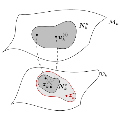
Figure 1: Extrapolation scenario for an in-situ-trained microscale HPROM: dark/light shaded area designates the region of the parameter space explored/unexplored during training.

There are two main approaches for detecting an extrapolation associated with the approximate solution of a queried microscale BVP characterized by $\bm{z}_{k}^{\star}$: a geometric approach that determines the position of $\bm{z}_{k}^{\star}$ in $\mathcal{D}_{k}$, relative to the sampled parameter points collected in $\bm{N}_{k}^{z}$; and a residual-based approach that computes the residual obtained when approximating the HDM-based solution of the queried microscale problem using a most-appropriate local HPROM.

The geometric approach is conceptually simple. However, its implementation is not trivial. It can be carried out by computing the hypersphere of smallest radius containing all parameter points collected in $\bm{N}_{k}^{z}$, or the minimal hyperpolygon connecting these parameter points, then checking whether $\bm{z}_{k}^{\star}$ lies or not within the hypersphere or hyperpolygon. Either implementation necessitates a fair amount of efficient computational geometry. In either case however, the main drawback of this approach is that if $\bm{z}_{k}^{\star}$ falls within either of the aforementioned target domains, this does not necessarily imply that the approximate solution computed using the most-appropriate local HPROM has an acceptable accuracy. Such information is provided however by the residual-based approach which, unlike the geometric approach, checks for potential extrapolation after rather than before the solution of the queried microscale BVP is computed. Specifically, this approach computes the following relative residual magnitude

$$r_{k}=\frac{\left\|\bm{f}_{k}\left(\bm{V}_{k}\bm{y}_{k},\stackrel{{\scriptstyle\circ}}{{\bm{u}}}_{k},\bm{\xi}_{k}\right)\right\|}{\left\|\bm{f}_{k}\left(\bm{0},\stackrel{{\scriptstyle\circ}}{{\bm{u}}}_{k},\bm{\xi}_{k}\right)\right\|}$$ (6)

and adopts it as an error indicator. When it exceeds a prescribed tolerance $r_{\text{tol}}$, it suggests discarding the approximate solution $\bm{V}_{k}\bm{y}_{k}$, enriching the most-appropriate local ROB $\bm{V}_{k}$, and repeating this process until $r_{k}\leq r_{\text{tol}}$. Hence, this alternative approach, which leads to the updating criterion outlined in Algorithm 1, equally applies for assessing extrapolation and interpolation errors.

Data: Queried parameter point $\bm{z}_{k}^{\star}\in\mathcal{D}_{k}$, and user-specified tolerance value $r_{\text{tol}}>0$

Result: Updating flag UF

1 Compute the approximate solution of the microscale BVP characterized by $\bm{z}_{k}^{\star}$ using the most-appropriate local HPROM

2 Compute the corresponding relative residual magnitude $r_{k}^{\star}$ (6)

3 if $r_{k}^{\star}>r_{\text{tol}}$ then

4       Solve the microscale BVP using the corresponding HDM

5       Collect the computed solution $\bm{u}_{k}^{\star}$ in $\bm{N}_{k}^{u}$

6       Sample the parameter point $\bm{z}_{k}^{\star}$ and collect it in $\bm{N}_{k}^{z}$

7       Set $\textrm{UF}=\textrm{true}$

8else

9       Accept the HPROM solution $\bm{u}_{k}^{\star}$

10       Set $\textrm{UF}=\textrm{false}$

Algorithm 1 Updating criterion for a database of local HPROMs.

4.2 Updating of a local reduced-order basis

Each update of a database $\mathcal{DB}_{k}$ starts by solving a new microscale BVP using the corresponding HDM, appending the computed solution $\bm{u}_{k}^{\star}$ to the current content of the relevant snapshot matrix $\bm{N}_{k}^{u}$, performing the Singular Value Decomposition (SVD) of $\bm{N}_{k}^{u}$, and deducing a new ROB using the singular value energy truncation criterion. Because the computational complexity of SVD applied to a rectangular matrix scales quadratically with the number of columns of the matrix, a low-rank SVD update method such as that presented in [24] is preferred here for compressing the collected snapshots.

For a highly nonlinear problem, the SVD and singular value energy truncation criterion configured for accuracy typically lead to a large ROB. Hence, if the size of such a ROB exceeds a specified capacity limit $c_{\text{max}}$, this ROB is split here into two smaller ROBs, each of which capable of capturing only the local behavior of a nonlinear microstructure. This splitting, which is bound in this context to occur recursively, leads to the concept of a local ROB. This concept is similar to that of local ROBs pioneered in [21] and equipped with the notion of clustering of solution snapshots. However, it differs from it in that locality refers here to the parameter space $\mathcal{D}_{k}$, whereas locality in [21] referred to the solution manifold (denoted here by ${\cal M}_{k})$. Indeed, the data collected in a parameter matrix $\bm{N}_{k}^{z}$ provides an alternative approach for building local ROBs by a mechanism centered around updating and splitting. Again, the updating criterion, which is proposed in this work for avoiding extrapolation, is described in Algorithm 1. Its basic principle is described in Algorithm 2. The proposed splitting algorithm is described below.

Data: Sampled parameter vector $\bm{z}_{k}^{\star}$ (or point in $\mathcal{D}_{k}$), corresponding HDM-based solution snapshot $\bm{u}_{k}^{\star}$, ROB $\bm{V}_{k}$, matrix of sampled deformation gradient parameter points $\bm{N}_{k}^{z}$, and snapshot matrix $\bm{N}_{k}^{u}$

Result: Updated ROB $\bm{V}_{k}$, updated sampled parameter matrix $\bm{N}_{k}^{z}$, and updated snapshot matrix $\bm{N}_{k}^{u}$

1 Update $\bm{N}_{k}^{z}\leftarrow\left[\bm{N}_{k}^{z}\quad\bm{z}_{k}^{\star}\right]$

2 Update $\bm{N}_{k}^{u}\leftarrow\left[\bm{N}_{k}^{u}\quad\bm{u}_{k}^{\star}\right]$

3 Perform low-rank SVD update of $\bm{N}_{k}^{u}$

4 Extract new (updated) ROB $\bm{V}_{k}$

Algorithm 2 Updating a ROB.

Specifically, $\bm{N}_{k}^{z}$ provides a mean for splitting a region of the parameter space $\mathcal{D}_{k}$ rather than a region of the solution space in two parts, using for example Principle Component Analysis (PCA) or POD, both of which build on SVD. PCA is most useful for exploratory data analysis. It is used here to compute the direction of maximum variance $\bm{n}_{k}$ of a set of sampled parameter points ${\cal S}_{z}^{m_{k}}$ as the first eigenvector of the covariance of the corresponding parameter matrix

$$\text{Cov}(\bm{N}_{k}^{z})=\bm{N}_{k}^{z}\bm{N}_{k}^{z^{T}}-\bar{\bm{z}}_{k}\bar{\bm{z}}_{k}^{T}$$ (7)

where $\bar{\bm{z}}_{k}\in\mathbb{R}^{n_{\mathrm{sd}}}$ is the columnwise mean of $\bm{N}_{k}^{z}$ – that is,

$$\bar{\bm{z}}_{k_{i}}=\displaystyle{\frac{1}{m_{k}}\sum_{j=1}^{m_{k}}\bm{N}_{k_{ij}}^{z},\qquad i=1,\ldots,n_{\mathrm{sd}}}$$ (8)

and therefore $\bar{\bm{z}}_{k}$ represents the algebraic centroid of the sampled parameter points.

Next, the hyperplane $\bm{h}_{k}$ containing the centroid point $\bar{\bm{z}}_{k}$ and orthogonal to $\bm{n}_{k}$ is constructed. This hyperplane can be described as

$$\bm{h}_{k}=\left\{\bm{x}|(\bm{x}-\bar{\bm{z}}_{k})^{T}\bm{n}_{k}=0\right\}$$ (9)

It naturally splits ${\cal S}_{z}^{m_{k}}$ into two smaller sets, where each partitioned set has a more compact spatial distribution in $\mathcal{D}_{k}$ (see Figure 2(b)).

As illustrated in Figure 2, the splitting of a set of sampled parameter points ${\cal S}_{z}^{m_{k}}$ into two smaller sets, which is equivalent to the partitioning of a matrix $\bm{N}_{k}^{z}$ into two smaller matrices, implies a splitting of a region of the parameter space $\mathcal{D}_{k}$. It also leads to the partitioning of the snapshot matrix $\bm{N}_{k}^{u}$ in two snapshot matrices. Finally, the compression of these two matrices leads in turn to the construction of two new local ROBs. The entire splitting process is summarized in Algorithm 3.

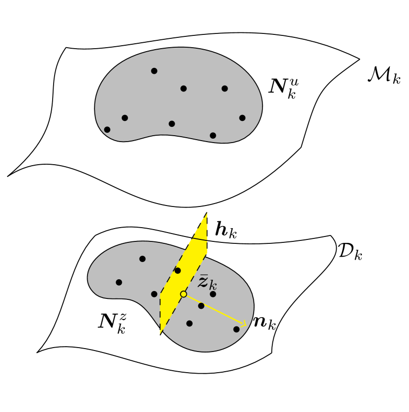
(a) splitting a set of sampled parameter points into two sets using a hyperplane

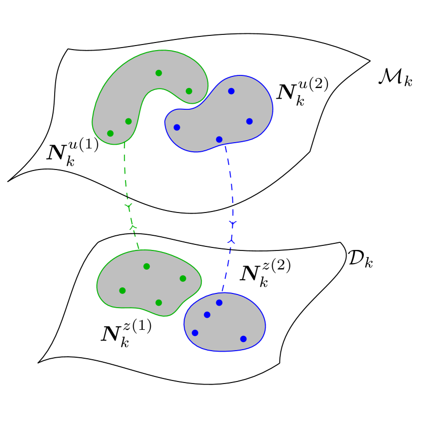
(b) partitioning the corresponding snapshot matrix into two matrices accordingly

Figure 2: Splitting a set of sampled parameter points in two sets in order to partition a snapshot matrix into two matrices and thereby split a ROB into two local ROBs.

Data: Matrix of sampled deformation gradient parameter points $\bm{N}_{k}^{z}$, snapshot matrix $\bm{N}_{k}^{u}$, and database of HPROM-related information $\mathcal{DB}_{k}$

Result: Split local ROBs $\bm{V}_{k}^{(1)}$ and $\bm{V}_{k}^{(2)}$, split parameter matrices $\bm{N}_{k}^{z^{(1)}}$ and $\bm{N}_{k}^{z^{(2)}}$, split snapshot matrices $\bm{N}_{k}^{u^{(1)}}$, and $\bm{N}_{k}^{u^{(2)}}$, and updated database $\mathcal{DB}_{k}$

1 Compute the first eigenvector $\bm{n}_{k}$ of the matrix $\text{Cov}(\bm{N}_{k}^{z})$ (7)

2 Construct the hyperplane $\bm{h}_{k}$ (9)

3 Using $\bm{h}_{k}$, partition $\bm{N}_{k}^{z}$ into two matrices $\bm{N}_{k}^{z^{(1)}}$ and $\bm{N}_{k}^{z^{(2)}}$

4 Partition $\bm{N}_{k}^{u}$ accordingly, into two matrices $\bm{N}_{k}^{u^{(1)}}$ and $\bm{N}_{k}^{u^{(2)}}$

5 Compute $\bm{V}_{k}^{(1)}$, $\bm{V}_{k}^{(2)}$ from $\bm{N}_{k}^{u^{(1)}}$, $\bm{N}_{k}^{u^{(2)}}$, respectively

6 Add $\bm{V}_{k}^{(1)}$, $\bm{N}_{k}^{z^{(1)}}$, $\bm{N}_{k}^{u^{(1)}}$, and $\bm{V}_{k}^{(2)}$, $\bm{N}_{k}^{z^{(2)}}$, $\bm{N}_{k}^{u^{(2)}}$ to the content of the database $\mathcal{DB}_{k}$

Delete $\bm{V}_{k}$, $\bm{N}_{k}^{z}$, $\bm{N}_{k}^{u}$ from the content of the database $\mathcal{DB}_{k}$

Algorithm 3 Splitting a ROB.

4.3 Approximation using a most-appropriate local ROB

The adaptive, in-situ sampling process described so far, which centers around updating and splitting ROBs, eventually leads to the presence of multiple local ROBs in a database $\mathcal{DB}_{k}$. Hence, when a microscale BVP characterized by an unsampled parameter point $\bm{z}_{k}^{\star}$ is queried for fast solution by a local HPROM, the most-appropriate local ROB available in $\mathcal{DB}_{k}$ must be identified online. This can be performed as proposed below.

Let $\mathcal{S}_{V}^{n_{k}}=\left\{\bm{V}_{k}^{(1)},\ldots,\bm{V}_{k}^{(n_{k})}\right\}$ denote the set of all $n_{k}$ local ROBs that are pre-computed and stored at a given time in a database $\mathcal{DB}_{k}$. Recall from Section 4 that each HDM-based solution $\bm{u}_{k}^{(i)}$ of a microscale BVP is associated with a parameter point $\bm{z}_{k}^{(i)}$ of the parameter space $\mathcal{D}_{k}$ that characterizes the BVP. Hence, a split snapshot matrix $\bm{N}_{k}^{u^{(l)}}$ can be associated on the same basis with a split parameter matrix $\bm{N}_{k}^{z^{(l)}}$. Similarly, a local ROB $\bm{V}_{k}^{(l)}$ can be associated with the snapshot matrix $\bm{N}_{k}^{u^{(l)}}$ that was compressed to obtain $\bm{V}_{k}^{(l)}$, and by transitivity, with the split parameter matrix $\bm{N}_{k}^{z^{(l)}}$.

Let $\bar{\bm{z}}_{k}^{(l)}$ denote the algebraic centroid of the parameter matrix $\bm{N}_{k}^{z^{(l)}}$ (defined as in (8)). Following the same reasoning as above, it follows that $\bar{\bm{z}}_{k}^{(l)}$ can be associated with the local ROB $\bm{V}_{k}^{(l)}$. More generally, a bijection can be defined between the set of sampled parameter points $\bar{\bm{z}}_{k}^{(l)}$ and the set of pre-computed local ROBs $\bm{V}_{k}^{(l)}$.

Now, given a queried BVP characterized by an unsampled deformation gradient parameter point $\bm{z}_{k}^{\star}$ – or more simply, given a queried but unsampled parameter point $\bm{z}_{k}^{\star}$ – a most-appropriate, pre-computed, local ROB $\bm{V}_{k}^{(j_{k})}\in\mathcal{S}_{V}^{n_{k}}$ – that is, $j_{k}\in\left\{1,\ldots,n_{k}\right\}$, can be defined as the pre-computed local ROB whose corresponding parameter point is the closest to the queried but unsampled parameter point $\bar{\bm{z}}_{k}^{\star}$ – that is,

$$j_{k}=\underset{i\in\left\{1,\ldots,n_{k}\right\}}{\operatorname{argmin}}\quad\left\|\bar{\bm{z}}_{k}^{(i)}-\bm{z}_{k}^{\star}\right\|$$

where $\|~{}\|$ denotes any preferred norm, for example, $\|~{}\|_{2}$.

4.4 Summary: in-situ adaptive microscale PMOR framework

Algorithm 4 summarizes the in-situ, adaptive, PMOR framework proposed for the acceleration of the solution of the microscale BVPs at any level $k$, $k=1,\ldots,n_{s}$.

Data: User-specified residual tolerance $r_{\text{tol}}$, and user-specified ROB capacity limit $c_{\text{max}}$

Result: HDM/HPROM-based solutions of $\Pi_{j=0}^{k-1}\left|\mathcal{G}_{j}\right|$ microscale BVPs at level $k$, and database of HPROM-related information $\mathcal{DB}_{k}$

1 Initialize $m_{k}$

2 Collect $\bm{N}_{k}^{z}$ and $\bm{N}_{k}^{u}$ and compute $\bm{V}_{k}$ using the in-situ training strategy described in Section 3.2

3 Initialize the content of $\mathcal{DB}_{k}$ with $\bm{V}_{k}$, $\bm{N}_{k}^{z}$ and $\bm{N}_{k}^{u}$

4 for solving each of the remaining $\prod_{j=0}^{k-1}\left|\mathcal{G}_{j}\right|-m_{k}$ microscale BVPs do

5       Compute the deformation gradient parameter point $\bm{z}_{k}^{\star}$

6       Identify in $\mathcal{DB}_{k}$ the corresponding most-appropriate local ROB $\bm{V}_{k}^{(j_{k})}$

7       Apply Algorithm 1 to update or not $\mathcal{DB}_{k}$

8       if UF = true (see Algorithm 1) then

9             Update $\mathcal{DB}_{k}$ using Algorithm 2

10             if size of updated ROB $>c_{\text{max}}$ then

11                   Split ROB using Algorithm 3

12            else

13                   Continue (to the next microscale BVP)

14                  

15            

16      else

17             Continue (to the next microscale BVP)

18            

19      

Algorithm 4 In-situ, adaptive, PMOR framework for the microscale BVPs at level $k$.

5 Applications

Here, the computational feasibility as well as the performance of the in-situ, adaptive, PMOR framework for microscale BVPs are demonstrated for two nonlinear, nonparametric, dynamic, two-scale simulations ($n_{s}=1$). Specifically, this framework is applied to the solution of two academic but nevertheless computationally intensive, nonlinear, two-level, dynamic response problems. For both applications, all ROBs are constructed using POD based on displacement solution snapshots. Because adaptive hyperreduction is beyond the scope of this paper, all HPROMs are constructed based on a single reduced mesh that is trained and generated using ECSW during the initialization step of Algorithm 4. Given that at the macroscale level neither considered problem is parametric, PMOR is applied in both cases only to the microscale model. This setting has two benefits:

• It enables the exclusive focusing on the performance of the proposed in-situ, adaptive approach for performing the PMOR of microscale problems.

• It corresponds to the worst case scenario of PMOR performance, as any computational overhead incurred by the PMOR process may only be amortized in this case by the same simulation to which the PMOR process is applied. Hence, any reported speedup factor is a genuine speedup factor.

Since both applications considered herein involve two-scale simulations ($n_{s}=1$), the model labels PROM and HPROM refer throughout the remainder of this section to the microscale computational model. On the other hand, the label HDM may refer to either the macroscale or the microscale computational model.

In both applications, the tolerance for the residual-based error indicator is set to $r_{\text{tol}}=0.001$, and the capacity limit for the dimension of a local ROB is set to $c_{\text{max}}=20$. The accuracy of all PROM and HPROM approximations is evaluated using the following definition of a relative global error

$$e_{\text{rel}}=\left|\frac{\sum\limits_{t\in P}\Delta s\left(\bm{u}_{\diamond}(t)-\tilde{\bm{u}}_{\diamond}(t)\right)^{T}\bm{1}}{\sum\limits_{t\in P}\Delta s\bm{u}_{\diamond}^{T}(t)\bm{1}}\right|\times 100\%$$

where the $\diamond$ subscript designates the $x$, $y$, or $z$ direction of a global reference frame, $\bm{u}_{\diamond}(t)\in\mathbb{R}^{n_{0}^{d}}$ is the vector of $\diamond$-displacements at time $t$ extracted from the macroscale solution based on HDMs at both the macroscale and microscale levels, $\tilde{\bm{u}}_{\diamond}(t)\in\mathbb{R}^{n_{0}^{d}}$ is the vector of $\diamond$-displacements at time $t$ extracted from the macroscale solution but based on a PROM or HPROM at the microscale level, $\Delta s$ is the error sampling time-step size, $\bm{1}$ denotes the vector of 1 entries, and $P$ is the set of time-stamps

$$P=\left\{t_{0},t_{0}+\Delta s,t_{0}+2\Delta s,\ldots,t_{f}\right\}$$

where $t_{0}$ is the initial simulated time and $t_{f}$ is the final simulated time.

All computations reported herein are performed on a Linux cluster with 84 compute nodes, dual-socket Intel Xeon E5-2650 v2 CPUs (8 cores/socket), 64 GB of DDR3 memory/node, a 1:1 subscribed FDR Infiniband network, and a Lustre shared file system tuned for parallel I/O.

For both applications, all reported PROM and HPROM wall-clock timings as well as speedup factors account for all training costs.

5.1 Vibration of a nonlinear solid elastic bar with a microvoid structure

A computational model for a solid bar made of a heterogeneous structure is considered here. At the finest scale, this structure is characterized by microscopic voids and a porosity ratio of $0.5$ (here, the porosity ratio is defined as the ratio of the total volume occupied by the voids, and the total volume occupied by the material and the voids). The bar has a solid square cross section of height and width $H=1$ cm, and a length $L=20$ cm. It is fixed at both ends. A distributed external force generated by a uniform pressure of magnitude $p=100$ MPa is suddenly applied on its upper face and oriented initially in the transverse direction. Due to symmetry, only half of the bar along its length is modeled.

At the microscale level, a FE model of the bar (see Figure 3) is constructed using 648 eight-noded hexahedral elements with three displacement DOFs per node. The dimension of this HDM is $n_{1}^{d}=1,962$ (1,962 DOFs). At this level, the material response is assumed to be well represented by a compressible neo-Hookean (finite strains) hyperelastic constitutive law with Young’s modulus $E=207$ GPa and Poisson’s ratio $\nu=0.3$. Uniform essential boundary conditions are adopted at this level.

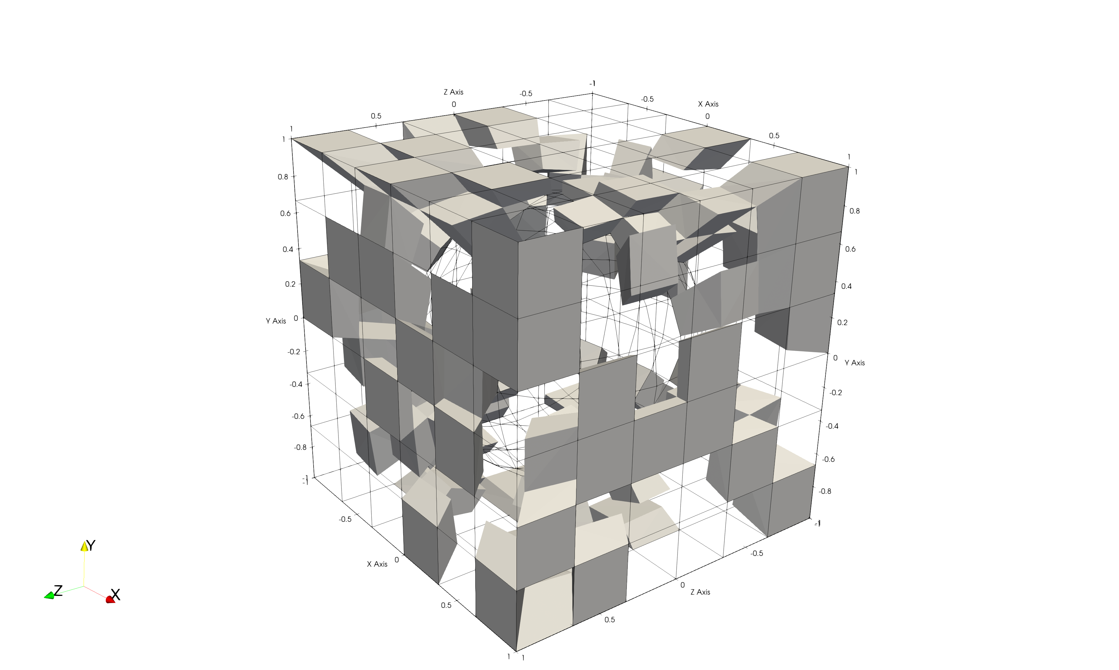
Figure 3: Vibration of a nonlinear solid elastic bar with a microvoid structure: FE mesh underlying the microscale HDM (wireframes) and associated ECSW-generated reduced mesh (shaded elements).

At the macroscale level, a FE model of the bar (see Figure 4) is constructed using 640 eight-noded hexahedral elements with three displacement DOFs/node, and a total number of $2,975$ DOFs ($n_{0}^{d}=2,975$). At this level, the material density is $\rho_{0}=7,830$ kg/m³, and temporal discretization is performed using the explicit central difference scheme and the constant time-step $\Delta t=3.25\times 10^{-7}$ s. The response of the bar is computed from $t_{0}=0$ s until $t_{f}=1\times 10^{-2}$ s.

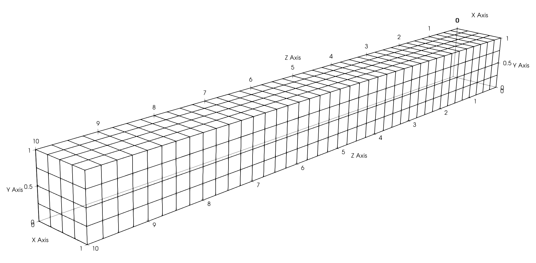
Figure 4: Vibration of a nonlinear solid elastic bar with a microvoid structure: FE mesh underlying the macroscale HDM.

First, an initial nonlinear PROM is constructed for the microscale computational model using the solution snapshots collected at $t_{0}=0$ s during the HDM-based solution of the first $m_{1}=500$ microscale BVPs encountered at the Gauss points of the macroscale computational model. Then, this PROM is hyperreduced using ECSW configured with the Lawson and Hanson sparse NNLS algorithm and a relative accuracy threshold $\varepsilon=10^{-3}$, which generates a reduced mesh with 115 elements (${\widetilde{\cal E}}=115$).

Several simulations are performed for this problem using: the macroscale and microscale HDMs described above; the proposed in-situ, adaptive, microscale PMOR framework, with and without hyperreduction (the reader is reminded that in this work, any reduced mesh generated by ECSW-based hyperreduction is not updated); and the counterpart nonadaptive microscale PMOR framework described in [9], with and without hyperreduction.

Table 1(a) reports the speedup factors and relative global errors computed using the error sampling time-step $\Delta s=\Delta t$ measured for the proposed in-situ, adaptive, microscale PMOR with and without hyperreduction. Similarly, Tables 1(b)–1(d) report these performance results for the counterpart in-situ, nonadaptive, microscale PMOR framework previously proposed in [9]. Since the latter framework depends in this case on the ad-hoc parameter $n_{0}^{\mathcal{G}}$ specifying the number of microscale BVPs to solve in order to train a global microscale PROM and the corresponding HPROM, three different values of this parameter are considered. The first one, $n_{0}^{\mathcal{G}}=62$, corresponds to 0.2% of the total number $n_{ms}$ of microscale problems solved during the multiscale simulation performed in the time-interval $[0,1\times 10^{-2}]$ s using the time-step size $\Delta t=3.25\times 10^{-7}$ s. The second and third values, $n_{0}^{\mathcal{G}}=154$ and $n_{0}^{\mathcal{G}}=308$, correspond to 0.5% of $n_{ms}$ and 1% of $n_{ms}$, respectively. From the results reported in this table, the following observations are noteworthy:

• In all cases, the HPROM delivers a much better speedup factor than its underlying PROM. This is expected given that the problem considered here is geometrically nonlinear (finite strains).

• The speedup factors delivered by all HPROMs are impressive, considering that the macroscale model is not even reduced.

• The adaptively computed PROM delivers 6 to 50 times more accurate results than its nonadaptive counterparts trained with any considered value of $n_{0}^{\mathcal{G}}$, and performs about 1.25 times faster.

• The adaptively computed HPROM – except for the nonadapted but fixed reduced mesh – delivers 2 to 3 times more accurate results than its nonadaptive counterpart trained with $n_{0}^{\mathcal{G}}=62$, but is 1.35 times slower. It delivers roughly the same wall-clock time performance as its nonadaptive counterpart trained with $n_{0}^{\mathcal{G}}=154$, and about the same accuracy. On the other hand, it is about 1.2 times faster than its nonadaptive counterpart trained with $n_{0}^{\mathcal{G}}=308$, while delivering essentially the same accuracy.

It follows that in all considered cases, the adaptive PROM is faster than its nonadaptive counterpart and considerably more accurate. On the other hand, because the reduced mesh resulting from the ECSW-based hyperreduction is fixed in this work, the otherwise adaptive HPROM can be anywhere from slightly slower to slightly faster than its nonadaptive counterpart, and roughly as accurate.

Considering that all aforementioned performance results account for all computational overhead, including the adaptation overhead, and that the proposed in-situ, adaptive, microscale PMOR framework is fully automated, these results demonstrate not only the feasibility of this framework but also its superiority over its nonadaptive counterpart. In particular, Figure 5 shows that even when the reduced mesh underlying the microscale computational model is not adapted, the proposed adaptive framework delivers a remarkable accuracy.

Table 1: Vibration of a nonlinear solid elastic bar with a microvoid structure: performance assessment.

Model	Wall-clock time (s)	Speedup factor
HDM	$1.35\times 10^{5}$	N.A.
PROM	$3.75\times 10^{4}$	$3.60$
HPROM	$8.92\times 10^{3}$	$15.2$
Error measure $e$	PROM	HPROM
y-displacement (%)	$0.0227$	$0.440$
z-displacement (%)	$0.0435$	$0.747$
y-velocity (%)	$0.103$	$1.77$
z-velocity (%)	$0.986$	$6.68$

(a) Adaptive

Model	Wall-clock time (s)	Speedup factor
HDM	$1.35\times 10^{5}$	N.A.
PROM	$4.64\times 10^{4}$	$3.03$
HPROM	$6.58\times 10^{3}$	$20.5$
Error measure $e$	PROM	HPROM
y-displacement (%)	$1.23$	$1.27$
z-displacement (%)	$2.11$	$2.59$
y-velocity (%)	$3.05$	$3.23$
z-velocity (%)	$9.52$	$10.6$

(b) Nonadaptive ($n_{0}^{\mathcal{G}}=62$)

Model	Wall-clock time (s)	Speedup factor
HDM	$1.35\times 10^{5}$	N.A.
PROM	$4.54\times 10^{4}$	$2.97$
HPROM	$8.71\times 10^{3}$	$15.5$
Error measure $e$	PROM	HPROM
y-displacement (%)	$0.0530$	$0.134$
z-displacement (%)	$0.106$	$0.219$
y-velocity (%)	$1.11$	$1.21$
z-velocity (%)	$6.24$	$6.50$

(c) Nonadaptive ($n_{0}^{\mathcal{G}}=154$)

Model	Wall-clock time (s)	Speedup factor
HDM	$1.35\times 10^{5}$	N.A.
PROM	$4.68\times 10^{4}$	$2.88$
HPROM	$1.06\times 10^{4}$	$12.7$
Error measure $e$	PROM	HPROM
y-displacement (%)	$0.0271$	$0.108$
z-displacement (%)	$0.0762$	$0.155$
y-velocity (%)	$1.10$	$1.03$
z-velocity (%)	$6.07$	$5.79$

(d) Nonadaptive ($n_{0}^{\mathcal{G}}=308$)

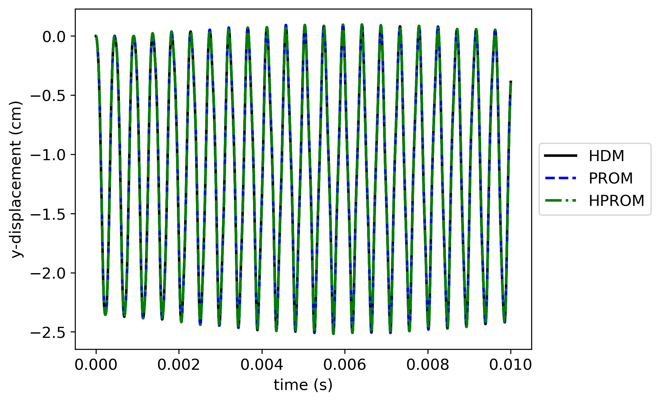
(a) displacement

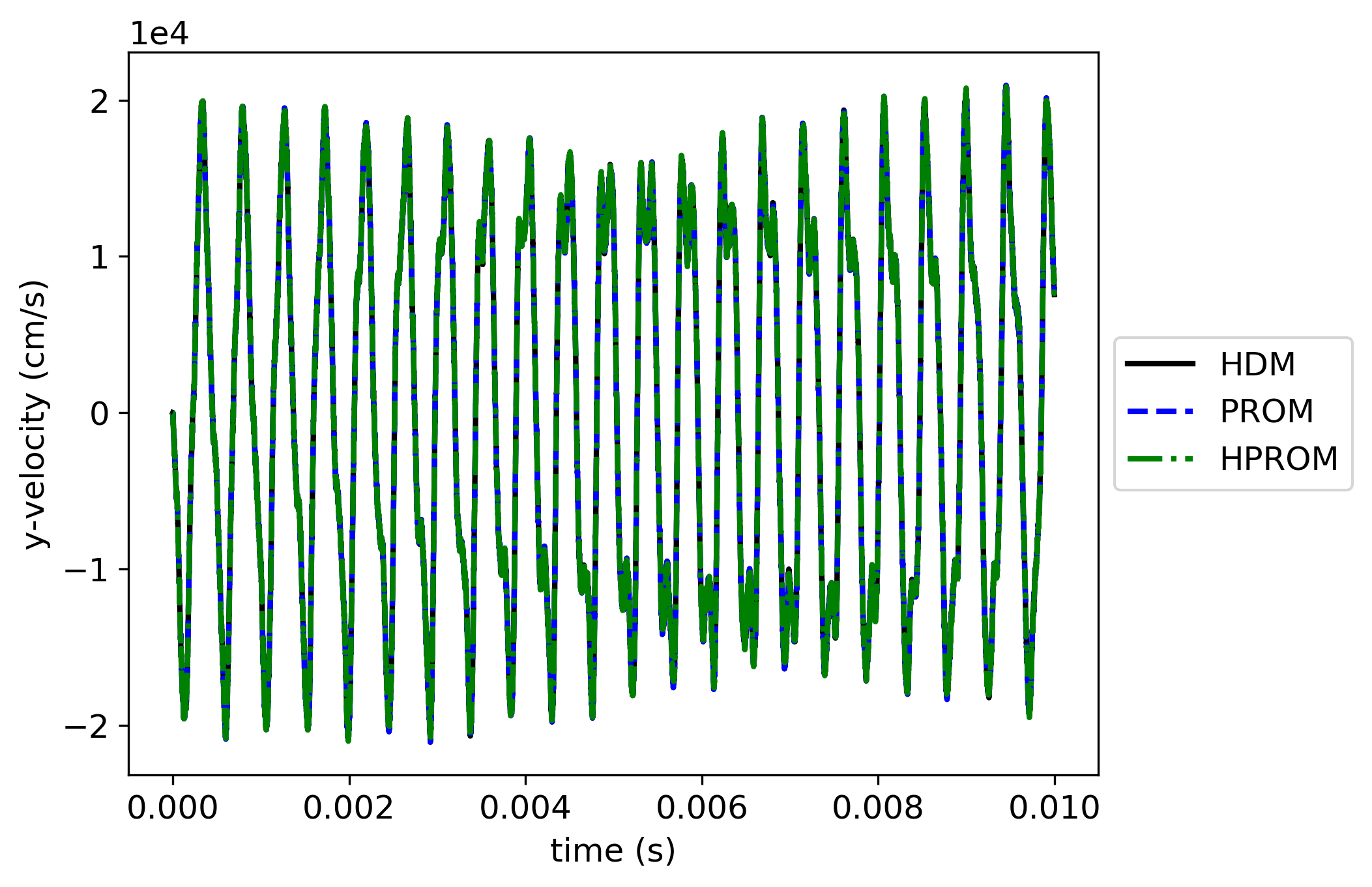
(b) velocity

Figure 5: Vibration of a nonlinear solid elastic bar with a microvoid structure – time-histories of a displacement DOF and a velocity DOF at a node of the mesh underlying the macroscale HDM computed using: the macroscale and microscale HDMs; and the in-situ, adaptive, microscale framework for PMOR with and without hyperreduction.

5.2 Impact of a nonlinear elastic cylinder with a composite microstructure on a rigid wall

Next, a computational model is considered for a cylindrical projectile with a heterogeneous microscale structure characterized by a stiff, unidirectional fiber embedded in a flexible matrix. The cylinder has a radius $R=0.476$ cm and a length $L=1.27$ cm. It has an initial velocity $v=15,000$ cm$/$s in the negative $z$-direction, and a frictionless rigid wall boundary condition at $z=0$. Due to symmetry, only one quarter of the bar along its length is modeled. This problem is a variant of the so-called Taylor impact problem [25].

For this problem, a FE microscale computational model is constructed using $729$ eight-noded hexahedral elements with three displacement DOFs per node, and a total number of $2,988$ DOFs. Uniform essential boundary conditions are adopted at this level. The microscale material is modeled as follows:

• The fiber is represented as a compressible neo-Hookean (finite strains) material with Young’s modulus $E=212.52\times 10^{10}$ dyne$/$cm² and Poisson’s ratio $\nu=0.4$. It runs parallel to the local $x$-axis along the center of the cube where the locally attached microstructure is defined. Its cross section is approximated by a square of edge size equal to one-third of the unit cell width.

• The flexible matrix surrounding this fiber is also represented as a compressible neo-Hookean material (finite strains), but with Young’s modulus $E=72.52\times 10^{10}$ dyne$/$cm² and Poisson’s ratio $\nu=0.4$.

At the macroscale level, a FE model is constructed using $1,008$ eight-noded hexahedral elements with three displacement DOFs/node, and a total number of $1,342$ DOFs (see Figure 6). At this level, the density is $\rho_{0}=2.7$ g/cm³. Temporal discretization is performed using the explicit central difference scheme and the constant time-step $\Delta t=1.0\times 10^{-9}$ s. For this problem, the multiscale simulation is performed from $t_{0}=0$ s until $t_{f}=1\times 10^{-6}$ s.

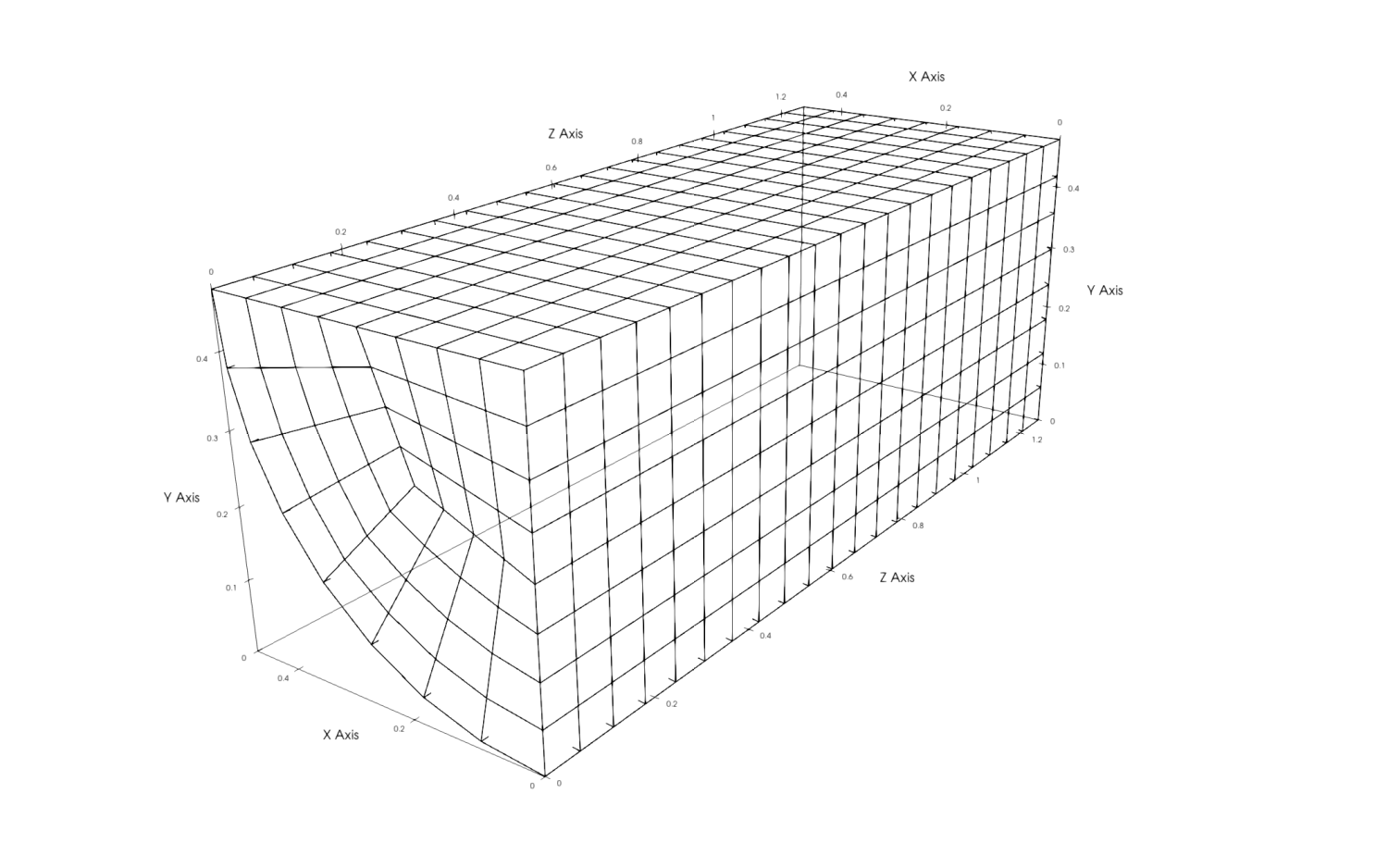
Figure 6: Impact on a rigid wall of a nonlinear elastic cylinder with a composite microstructure: FE mesh underlying the macroscale HDM.

As in the previous application, the proposed in-situ, adaptive, microscale framework for PMOR is initialized with the construction of a nonlinear PROM based on the first $m_{1}=500$ HDM-based solutions of the microscale BVPs encountered at the Gauss points of the macroscale computational model. Then, this PROM is hyperreduced using ECSW configured with the same sparse NNLS algorithm as in the previous application, and the same threshold for relative accuracy $\varepsilon=10^{-3}$. ECSW generates in this case a reduced mesh with 88 elements (${\widetilde{\cal E}}=88$). Three multiscale computations are performed using: the aforementioned macroscale and microscale HDMs; and the proposed in-situ, adaptive, microscale PMOR framework, with and without hyperreduction. The obtained performance results are reported in Table 2, where the relative global errors are computed with $\Delta s=\Delta t$.

Figure 7 displays two sample time-histories computed for a displacement DOF and a velocity DOF at a same node of the macroscale FE model. It shows that both adaptive PROM and HPROM reproduce extremely accurately the predictions obtained using the macroscale and microscale HDMs. This impressive accuracy of the proposed adaptive PMOR framework is confirmed by the quantitative error results reported in Table 2. This table also shows that for the application considered herein, the in-situ, adaptive, microscale framework for PMOR with and without hyperreduction accelerates the time to solution of the simulation based on the macroscale and microscale HDMs by a factor greater than 7. Again, this is an excellent performance result considering that it accounts for the computational time elapsed in the processing of the macroscale model, which is neither reduced nor hyperreduced, and accounts for all computational overhead associated with the PMOR process – including adaptation.

Table 2: Impact on a rigid wall of a nonlinear elastic cylinder with a composite microstructure: performance assessment of the in-situ, adaptive, microscale framework for PMOR with and without hyperreduction.

Model	Wall-clock time (s)	Speedup factor	Error measure $e$	PROM	HPROM
HDM	$2.44\times 10^{4}$	N.A.	$x$-displacement (%)	$0.00185$	$0.000467$
PROM	$1.60\times 10^{4}$	$1.52$	$y$-displacement (%)	$0.000165$	$0.000350$
HPROM	$3.34\times 10^{3}$	$7.3$	$x$-velocity (%)	$0.000449$	$0.00851$
			y-velocity (%)	$0.000430$	$0.00991$

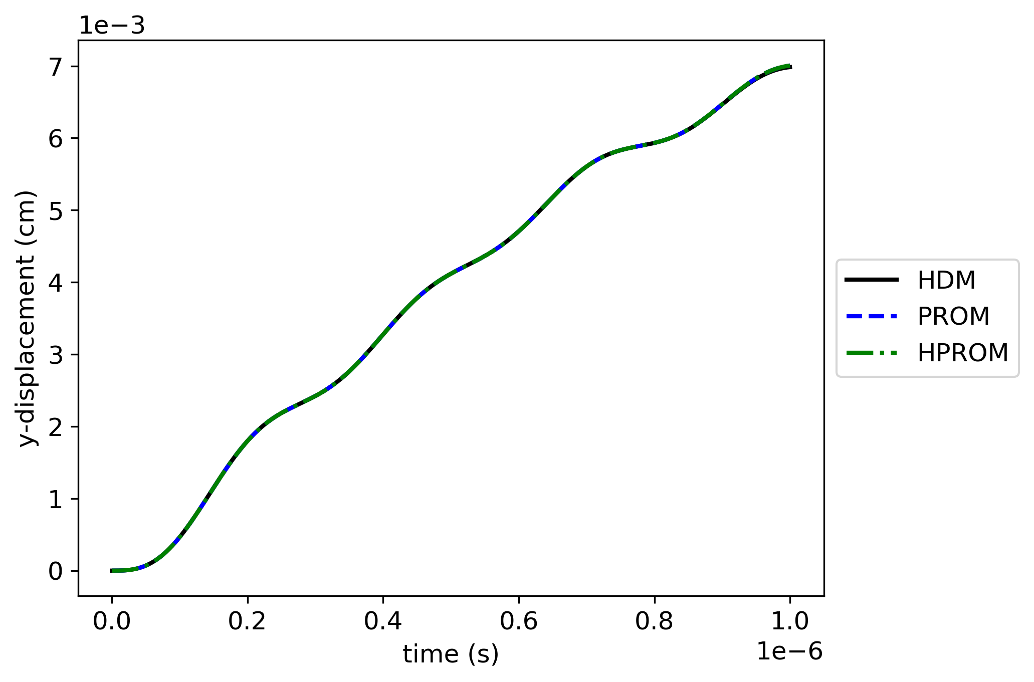
(a) Displacement

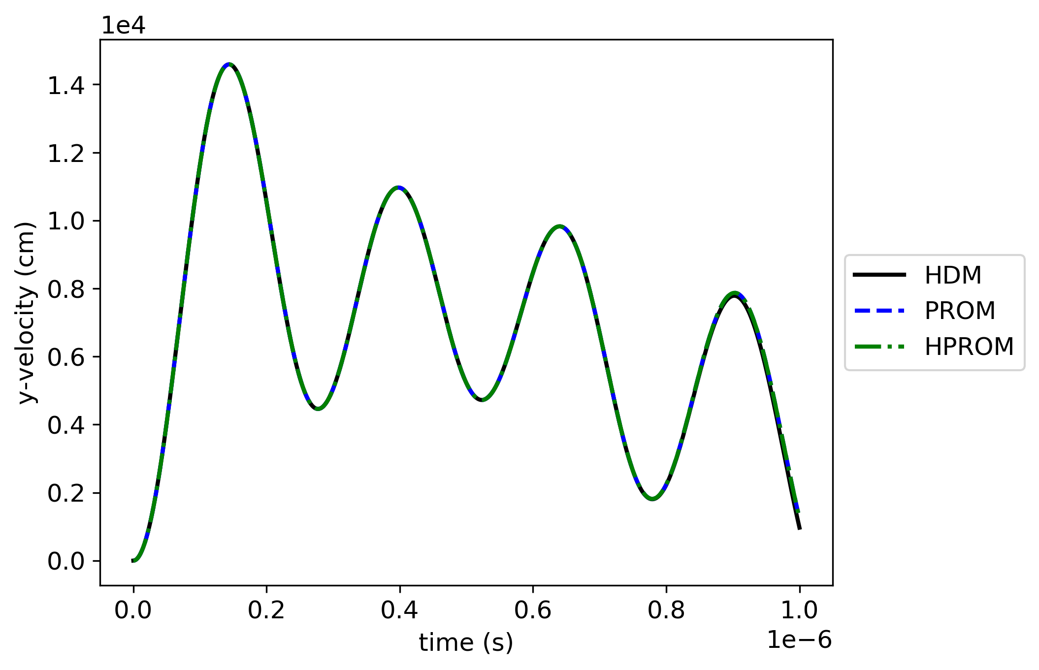
(b) Velocity

Figure 7: Impact on a rigid wall of a nonlinear elastic cylinder with a composite microstructure – time-histories of a displacement DOF and a velocity DOF at a node of the mesh underlying the macroscale HDM computed using: the macroscale and microscale HDMs; and the in-situ, adaptive, microscale framework for PMOR with and without hyperreduction.

6 Conclusions

An in-situ, adaptive, microscale Projection-based Model Order Reduction (PMOR) framework is proposed in this paper for accelerating the simulation of the nonlinear dynamics of multiscale structural and solid mechanics systems. It is designed to avoid by construction the weakness of extrapolation typically found in nonadaptive training methods. This framework is based on the parameterization of the deformation gradient for the purpose of PMOR at all but the coarsest scale, and on the concept of a database of local Reduced-Order Bases (ROBs) where locality is measured in the deformation gradient parameter space. It achieves accuracy by sampling new high-dimensional information as needed, updating on-the-fly a constructed ROB, and approximating the solution along its trajectory using a handbook of most-appropriate local ROBs. It achieves computational efficiency by splitting an updated ROB that becomes larger than desired into two local ones, each capable of capturing only the local behavior of a nonlinear mesostructure or microstructure, and incorporating hyperreduction (albeit without adaptivity). If the macroscale computational model is not a parametric one, it is not reduced. Even in this case – that is, when the macroscale computational model is high-dimensional and its computational cost is accounted for – and when all computational overhead associated with performing PMOR and its adaptation are also accounted for, the proposed in-situ, adaptive, PMOR framework accelerates three-dimensional, nonlinear, dynamic, multiscale simulations of the academic type by roughly an order of magnitude without compromising accuracy. Larger speedup factors can be expected for more realistic, large-scale problems and when adaptivity is extended to hyperreduction.

While described in the context of nonlinear, multiscale, dynamic problems in solid mechanics and structural dynamics, the proposed in-situ, adaptive, PMOR framework is sufficiently comprehensive to be tailorable to many other applications. Indeed, conventional offline training of ROBs in a predetermined region of a parameter space typically leads to parametric reduced-order models that are bound to perform some form of extrapolation, whenever they are exercised in a region of the parameter space that was not explored during training. The proposed framework is designed specifically to remedy this issue.

References

- Qiao et al. [2008] Qiao P, Yang M, Bobaru F. Impact mechanics and high-energy absorbing materials. Journal of Aerospace Engineering 2008;21(4):235–248.
- Ma and Zhu [2017] Ma E, Zhu T. Towards strength–ductility synergy through the design of heterogeneous nanostructures in metals. Materials Today 2017;20(6):323–331.
- Hoffler et al. [2000] Hoffler C, Moore K, Kozloff K, Zysset P, Brown M, Goldstein S. Heterogeneity of bone lamellar-level elastic moduli. Bone 2000;26(6):603–609.
- Mei and Vernescu [2010] Mei CC, Vernescu B. Homogenization methods for multiscale mechanics. World scientific; 2010.
- Smit et al. [1998] Smit R, Brekelmans W, Meijer H. Prediction of the mechanical behavior of nonlinear heterogeneous systems by multi-level finite element modeling. Computer methods in applied mechanics and engineering 1998;155(1-2):181–192.
- Miehe et al. [1999] Miehe C, Schröder J, Schotte J. Computational homogenization analysis in finite plasticity simulation of texture development in polycrystalline materials. Computer methods in applied mechanics and engineering 1999;171(3-4):387–418.
- Feyel and Chaboche [2000] Feyel F, Chaboche JL. FE2 multiscale approach for modelling the elastoviscoplastic behaviour of long fibre SiC/Ti composite materials. Computer methods in applied mechanics and engineering 2000;183(3-4):309–330.
- Kouznetsova et al. [2001] Kouznetsova V, Brekelmans W, Baaijens F. An approach to micro-macro modeling of heterogeneous materials. Computational mechanics 2001;27(1):37–48.
- Zahr et al. [2017] Zahr MJ, Avery P, Farhat C. A multilevel projection-based model order reduction framework for nonlinear dynamic multiscale problems in structural and solid mechanics. International Journal for Numerical Methods in Engineering 2017;112(8):855–881.
- Sirovich [1987] Sirovich L. Turbulence and the dynamics of coherent structures. I. Coherent structures. Quarterly of applied mathematics 1987;45(3):561–571.
- LeGresley and Alonso [2000] LeGresley P, Alonso J. Airfoil design optimization using reduced order models based on proper orthogonal decomposition. In: Fluids 2000 conference and exhibit; 2000. p. 2545.
- Manzoni et al. [2012] Manzoni A, Quarteroni A, Rozza G. Shape optimization for viscous flows by reduced basis methods and free-form deformation. International Journal for Numerical Methods in Fluids 2012;70(5):646–670.
- Farhat et al. [2018a] Farhat C, Bos A, Tezaur R, Chapman T, Avery P, Soize C. A stochastic projection-based hyperreduced order model for model-form uncertainties in vibration analysis. In: 2018 AIAA Non-Deterministic Approaches Conference; 2018. p. 1410.
- Farhat et al. [2018b] Farhat C, Bos A, Avery P, Soize C. Modeling and quantification of model-form uncertainties in eigenvalue computations using a stochastic reduced model. AIAA Journal 2018;56(3):1198–1210.
- Hetmaniuk et al. [2012] Hetmaniuk U, Tezaur R, Farhat C. Review and assessment of interpolatory model order reduction methods for frequency response structural dynamics and acoustics problems. International Journal for Numerical Methods in Engineering 2012;90(13):1636–1662.
- Amsallem et al. [2010] Amsallem D, Cortial J, Farhat C. Towards real-time computational-fluid-dynamics-based aeroelastic computations using a database of reduced-order information. AIAA journal 2010;48(9):2029–2037.
- Yvonnet and He [2007] Yvonnet J, He QC. The reduced model multiscale method (R3M) for the non-linear homogenization of hyperelastic media at finite strains. Journal of Computational Physics 2007;223(1):341–368.
- Monteiro et al. [2008] Monteiro E, Yvonnet J, He QC. Computational homogenization for nonlinear conduction in heterogeneous materials using model reduction. Computational Materials Science 2008;42(4):704–712.
- Farhat et al. [2014] Farhat C, Avery P, Chapman T, Cortial J. Dimensional reduction of nonlinear finite element dynamic models with finite rotations and energy-based mesh sampling and weighting for computational efficiency. International Journal for Numerical Methods in Engineering 2014;98(9):625–662.
- Farhat et al. [2015] Farhat C, Chapman T, Avery P. Structure-preserving, stability, and accuracy properties of the energy-conserving sampling and weighting method for the hyper reduction of nonlinear finite element dynamic models. International Journal for Numerical Methods in Engineering 2015;102(5):1077–1110.
- Amsallem et al. [2012] Amsallem D, Zahr MJ, Farhat C. Nonlinear model order reduction based on local reduced-order bases. International Journal for Numerical Methods in Engineering 2012;92(10):891–916.
- Lawson and Hanson [1995] Lawson CL, Hanson RJ. Solving least squares problems, vol. 15. Siam; 1995.
- Chapman et al. [2017] Chapman T, Avery P, Collins P, Farhat C. Accelerated mesh sampling for the hyper reduction of nonlinear computational models. International Journal for Numerical Methods in Engineering 2017;109(12):1623–1654.
- Zahr and Farhat [2015] Zahr MJ, Farhat C. Progressive construction of a parametric reduced-order model for PDE-constrained optimization. International Journal for Numerical Methods in Engineering 2015;102(5):1111–1135.
- Taylor [1948] Taylor GI. The use of flat-ended projectiles for determining dynamic yield stress I. Theoretical considerations. Proceedings of the Royal Society of London Series A Mathematical and Physical Sciences 1948;194(1038):289–299.