[sakumoto@kwansei.ac.jp]Yusuke Sakumotomkwansei [aida@tmu.ac.jp]Masaki Aidaftmu-univ

[kwansei]Kwansei Gakuin University, 2-1 Gakuen, Sanda, Hyogo 669-1337, Japan [tmu-univ]Tokyo Metropolitan University, 6-6 Asahigaoka, Hino, Tokyo 191-0065, Japan

The Wigner’s Semicircle Law of Weighted Random Networks

The spectral graph theory provides an algebraical approach to investigate the characteristics of weighted networks using the eigenvalues and eigenvectors of a matrix (e.g., normalized Laplacian matrix) that represents the structure of the network. However, it is difficult for large-scale and complex networks (e.g., social network) to represent their structure as a matrix correctly. If there is a universality that the eigenvalues are independent of the detailed structure in large-scale and complex network, we can avoid the difficulty. In this paper, we clarify the Wigner’s Semicircle Law for weighted networks as such a universality. The law indicates that the eigenvalues of the normalized Laplacian matrix for weighted networks can be calculated from the a few network statistics (the average degree, the average link weight, and the square average link weight) when the weighted networks satisfy the sufficient condition of the node degrees and the link weights.

1 Introduction

Many networks (e.g., railway network, social network, the Internet, and airport network) are often modeled as weighted networks that are composed of nodes and weighted links [1, 2, 3]. The weighting of links is important to model a network, but it is hard for large-scale and complex networks such as social network. In the social network, nodes and links correspond to persons and their acquaintance relationships, respectively. In order to correctly give the weight for each link in the social network, the strength of the relationships among people should be accurately estimated from a huge amount of personal data (e.g., communication histories in mobile phone and social media). Due to the problem of the privacy and the computational complexity, it is unrealistic to gather such personal data, and calculate the strength of the relationships accurately.

The spectral graph theory provides an algebraical approach to investigate the characteristics of weighted networks using the eigenvalues and the eigenvectors of a matrix (e.g., normalized Laplacian matrix) that represents the structure of the network [4, 5]. In particular, the eigenvalues are important to understand the characteristics related to the entire network on the basis of the spectral graph theory. In [6], we have been clarified that the eigenvalue distribution of the normalized Laplacian matrix affects the information dissemination speed throughout the social network. In general, the eigenvalues of the matrix are calculated from all the matrix elements. For the matrix representing the structure of a weighted network, its elements are determined by the links weights. Hence, the weighting of the links is required to apply the spectral graph theory for weighted networks. This would be the barrier to apply the spectral graph theory for large-scale and complex networks due to the above-mentioned problems. However, the weighting of the links is avoidable if there is a universality that the eigenvalues are independent of the detailed structure (e.g., the weight of each link) of large-scale and complex networks. Therefore, the finding of such a universality of the eigenvalues expands the applicable region of the spectral graph theory.

The random matrix theory discusses a universality of the eigenvalues if the elements of the matrix are given by random variables [7, 8, 9]. In [9], Chung et al. have been analyzed the random matrix corresponding to the normalized Laplacian matrices for unweighted networks, and have clarified the universality (the Wigner’s semicircle law) that the eigenvalues of the normalized Laplacian matrix follow the semicircle distribution. To our knowledge, no study has clarified a universality of the eigenvalues for weighted networks.

In this paper, we clarify the universality (the Wigner’s semicircle law) of the eigenvalues for weighted networks on the basis of the discussion of  [9]. The clarified universality indicates that the eigenvalues of the normalized Laplacian matrix for weighted networks can be calculated from the a few network statistics (the average degree, the average link weight, and the square average link weight) when the weighted networks satisfy the sufficient condition of the node degrees and the link weights. Using some numerical examples, we confirm the validity of the sufficient condition.

This paper is organized as follows. In Sect. 2, we describe the spectral graph theory and the random matrix theory for weighted networks. In Sect. 3, we prove the Wigner’s semicircle law for weighted networks on the basis of the random matrix theory. Section 4 shows some numerical examples. Finally, in Sect. 5, we conclude this paper and discuss the future work.

2 Preliminary

2.1 Spectral Graph Theory

In the spectral graph theory, the structure of a network is represented by the matrix, and its characteristics is investigated using the eigenvalues and the eigenvectors of the matrix. In this section, we describe the spectral graph theory for weighted networks.

We denote a weighted network by $G=(V,E,\bm{w})$ where $V$ and $E$ are the sets of nodes and links, respectively. Let $n$ be the number of nodes in $G$. The link between nodes $i$ and $j$ is denoted by $(i,j)$. Link $(i,j)$ has the weight $w(i,j)$ where $w(i,j)=w(j,i)$ and $w(i,j)>0$. Let $\partial i$ be the set of adjacency nodes of node $i$. The weighted degree $d_{i}$ of nodes $i$ is defined by

$$d_{i}:=\sum_{j\in\partial i}w(i,j).$$ (1)

To represent the structure of links and nodes in $G$, there are adjacency matrix $\bm{A}$ and degree matrix $\bm{D}$, respectively. The $(i,j)$-th element $A(i,j)$ of adjacency matrix $\bm{A}$ is defined by

$$A(i,j):=\begin{cases}w(i,j)&\mathrm{if}\,(i,j)\in E\\ 0&\mathrm{otherwise}\end{cases}.$$ (2)

Degree matrix $\bm{D}$ is defined by

$$\bm{D}:={\rm diag}(d_{i})_{1\leq i\leq n}.$$ (3)

To represent the both structure of nodes and links in $G$, normalized Laplacian matrix $\bm{N}$ is often used. Normalized Laplacian matrix $\bm{N}$ is defined by

$$\bm{N} :=\bm{I}-\bm{D}^{-1/2}\bm{A}\bm{D}^{-1/2},$$ (4)

where $\bm{I}$ is the identity matrix.

Since normalized Laplacian matrix $\bm{N}$ is symmetric $(\bm{N}={\bm{N}}^{\mathsf{\!T}})$, its eigenvalue $\lambda_{l}$ ($l=1,...,n$) are real numbers. Let $\bm{q}_{l}$ be the eigenvector of eigenvalue $\lambda_{l}$ where ${\bm{q}_{l}}^{\mathsf{\!T}}\bm{q}_{l}=1$. We assign a number to $\lambda_{l}$ in ascending order, and hence $\lambda_{l}$ means the $l$-th minimum eigenvalue of $\bm{N}$. The range of the eigenvalues is given by

$$0=\lambda_{1}<\lambda_{2}\leq...\leq\lambda_{n}<2.$$ (5)

If $\lambda_{2}>0$, weighted network $G$ is connected (i.e., there is at least one path between every pair of nodes). Then, weighted network $G$ is not bipartite graph if $\lambda_{2}<2$. We define spectral radius $r$ by $r:=\max_{2\leq l\leq n}|1-\lambda_{l}|$. Spectral radius $r$ is in $0<r<1$ because $0<\lambda_{l}<2$ for $2\leq l\leq n$. Eigenvector $\bm{q}_{1}$ of minimum eigenvalue $\lambda_{1}$ is given by

$$\bm{q}_{1}=\frac{1}{\sqrt{{\rm Vol}(G)}}{(\sqrt{d_{1}},\sqrt{d_{2}},...,\sqrt{d_{n}})}^{\mathsf{\!T}},$$ (6)

where ${\rm Vol}(G)$ is defined by

$${\rm Vol}(G):=\sum_{i\in G}d_{i}.$$ (7)

Since eigenvector $\bm{q}_{l}$ is the orthonormal basis, matrix $\bm{Q}=(\bm{q}_{l})_{1\leq k\leq n}$ is the orthogonal matrix ($\bm{Q}^{-1}={\bm{Q}}^{\mathsf{\!T}}$).

Using $\bm{Q}$ and $\bm{\Lambda}={\rm diag}(\lambda_{l})_{1\leq k\leq n}$, normalized Laplacian matrix $\bm{N}$ is given by

$$\bm{N}=\bm{Q}\bm{\Lambda}{\bm{Q}}^{\mathsf{\!T}}=\sum_{l=1}^{n}\lambda_{l}\,\bm{q}_{l}\,{\bm{q}}^{\mathsf{\!T}}_{l}.$$ (8)

From the above equation, $\bm{N}$ is determined by eigenvalues $(\lambda)_{1\leq l\leq n}$ and eigenvectors $(\bm{q}_{l})_{1\leq l\leq n}$. Hence, weighted network $G$ can be analyzed not only with $\bm{N}$ but also with their eigenvalues and eigenvectors. The spectral graph theory provides an algebraical analysis method of $G$ with eigenvalues $\lambda_{l}$ and eigenvectors $\bm{q}_{l}$ of $\bm{N}$. In particular, eigenvalues $\lambda_{l}$ is important to understand the statistical characteristics related to the whole of weighted network $G$. In order to calculate eigenvalues $\lambda_{l}$, in general, all elements $N(i,j)$ must be given correctly. However, if there is a useful universality of eigenvalues $\lambda_{l}$, we can investigate the statistical characteristics of weighted network $G$ without all elements $N(i,j)$.

2.2 Random Matrix Theory

The random matrix theory focuses on random matrices that the elements are given by random variables, and clarifies that a universality of the eigenvalues appears if the matrix size approaches to infinity. When the links and their weights in weighted network $G$ are randomly given with a stochastic rule, elements $N(i,j)$ of normalized Laplacian matrix $\bm{N}$ become random variables, and $\bm{N}$ can be treated as a random matrix. Note that the universality of eigenvalues $\lambda_{l}$ of $\bm{N}$ corresponds to a characteristic of the statistical ensemble of the random networks generated with the same stochastic rule. Hence, clarifying such a universality contributes the growth of the statistical mechanics on networks.

In [9], the link between nodes $i$ and $j$ in unweighted networks is randomly generated using the stochastic rule with random variable $L_{ij}$. If $L_{ij}=0$, there is no link between nodes $i$ and $j$. On the other hand, if $L_{ij}=1$, the link exists between nodes $i$ and $j$. We denote probability $\mathbb{P}\left[L_{ij}=1\right]$ by $p_{ij}$, which is given by

$$p_{ij}=\rho\,\omega_{i}\,\omega_{j},$$ (9)

where $\omega_{i}>0$ and $\rho=1/\sum_{i\in V}\omega_{i}$. Using Eq. (9), the expectation of the node $i$’s degree is given by $\omega_{i}$. Let $\omega_{\rm avg}$, $\omega_{\rm min}$, and $\omega_{\rm max}$ be the average degree, the minimum degree, and the maximum degree. These are defined by $\omega_{\rm avg}:=1/n\sum_{i\in V}\omega_{i}$, $\omega_{\rm min}:=\inf_{i\in V}\omega_{i}$, and $\omega_{\rm max}:=\sup_{i\in V}\omega_{i}$, respectively. We can write $\rho$ by $\rho=1/(n\,\omega_{\rm avg})$. Similarly to [9], we assume that $\omega_{\rm max}^{2}<1/\rho$ so that $p_{ij}\leq 1$. As the scale of networks becomes large, the degrees of nodes are likely to become large. Hence, similarly to [9], we assume that $\omega_{\rm min}$ diverges to infinity as $n\rightarrow\infty$. Using the above stochastic rule, special networks (e.g., networks with no links) are rarely generated. However, the probability generating such special networks is very small, and hence this is no problem to discuss a universality appearing when $n\rightarrow\infty$.

In weighted network $G$, the weight of link $(i,j)$ is randomly set using the stochastic rule with random variable $W$. In the stochastic rule, random variable $W$ follows the conditional probability density function $f_{W\mid L_{ij}}(w\mid l)$, which is defined by

$$f_{W\mid L_{ij}}(w\mid l)\,{\rm d}w:=\mathbb{P}\left[w\leq W\leq w+{\rm d}w\mid L_{ij}=l\right].$$ (10)

If $L_{ij}=0$ (i.e., link $(i,j)$ does not exist), $W$ is always $0$, and hence $f_{W\mid L_{ij}}(w\mid 0)=\delta(w)$ where $\delta(x)$ is the Dirac delta function. On the contrary, if $L_{ij}=1$, $W>0$. Since link weights in actual networks cannot be infinity, we assume that $W$ is bounded. Using a finite value $w_{\rm max}$, $W\leq w_{\rm max}$. For the sake of convenience, we write

$$p_{W}(w):=f_{W\mid L_{ij}}(w\mid 1).$$ (11)

Let $\mathbb{E}_{p_{W}\!}\bigl{[}W^{m}\bigr{]}$ be the $m$-th moment of $W$ with the condition $L_{ij}=1$. $\mathbb{E}_{p_{W}\!}\bigl{[}W^{m}\bigr{]}$ is defined by

$$\mathbb{E}_{p_{W}\!}\bigl{[}W^{m}\bigr{]} :=\int_{0}^{w_{\rm max}}w^{m}\,p_{W}(w)\,{\rm d}w.$$ (12)

Even if the weights of all links in $G$ are divided by $w_{\rm max}$, normalized Laplacian matrix $\bm{N}$ is invariant. Hence, without loss of generality, we assume that $w_{\rm max}=1$. With this assumption, $\mathbb{E}_{p_{W}\!}\bigl{[}W^{m}\bigr{]}$ has the following properties: (a) $\mathbb{E}_{p_{W}\!}\bigl{[}W^{l}\bigr{]}\leq\mathbb{E}_{f_{W}\!}\bigl{[}W^{m}\bigr{]}$ for $l>m$, and (b) $\mathbb{E}_{p_{W}\!}\bigl{[}W^{m}\bigr{]}\leq 1$ since $\mathbb{E}_{p_{W}\!}\bigl{[}W^{0}\bigr{]}=1$.

Following the above stochastic rules, not only elements $N(i,j)$ but also eigenvalues $\lambda_{l}$ ($l=2,...,n$) of the normalized Laplacian matrix $\bm{N}$ for the weighted network $G$ become random variables depending on the set of random variables $\bm{\Gamma}=(\bm{L},W)$ where $\bm{L}=(L_{ij})_{(i,j)\in V^{2}}$. Let $\Lambda$ be the random variable for eigenvalue $\lambda$ of $\bm{N}$. We denote the conditional eigenvalue density of eigenvalues $\lambda_{l}$ ($l=2,...,n$) of $\bm{N}$ by $f_{\bm{\Lambda}\mid\bm{\Gamma}}^{(n)}(\lambda\mid\gamma)$, which is defined by

$$f_{\Lambda\mid\bm{\Gamma}}^{(n)}(\lambda\mid\bm{\gamma}):=\frac{1}{n-1}\sum_{l=2}^{n}\delta\left(\lambda-\lambda_{l}\right),$$ (13)

where $\lambda_{l}$ is the function of $\bm{\gamma}$. Since eigenvalues $\lambda_{l}$ vary stochastically, conditional eigenvalue density $f_{\Lambda\mid\bm{\Gamma}}^{(n)}(\lambda\mid\bm{\gamma})$ is also a random variable. Note that $f_{\Lambda\mid\bm{\Gamma}}^{(n)}(\lambda\mid\bm{\gamma})$ can be treated as a conditional probability density function because $\int_{\lambda_{2}}^{\lambda_{n}}f_{\Lambda\mid\bm{\Gamma}}^{(n)}(\lambda\mid\bm{\gamma})\,{\rm d}\lambda=1$. Using probability $\mathbb{P}\left[\bm{\Gamma}=\bm{\gamma}\right]$, eigenvalue density $f_{\Lambda}^{(n)}(\lambda)$ of $\bm{N}$ is given by

$$f_{\Lambda}^{(n)}(\lambda) =\mathbb{E}_{\mathbb{P}\left[\bm{\Gamma}\right]\!}\bigl{[}f_{\Lambda\mid\bm{\Gamma}}^{(n)}(\lambda\mid\bm{\gamma})\bigr{]}$$

$$=\frac{1}{n-1}\sum_{\bm{\gamma}}\mathbb{P}\left[\bm{\Gamma}=\bm{\gamma}\right]\sum_{l=2}^{n}\delta\left(\lambda-\lambda_{l}\right).$$ (14)

Since $\int_{\lambda_{2}}^{\lambda_{n}}f_{\Lambda}^{(n)}(\lambda)\,{\rm d}\lambda=1$, $f_{\Lambda}^{(n)}(\lambda)$ can be also treated as a probability density function. Then, we denote the $m$-th moment for $1-\Lambda$ using $f_{\Lambda}^{(n)}(\lambda)$ by $\mathbb{E}_{f^{(n)}_{\Lambda}\!}\bigl{[}(1-\Lambda)^{m}\bigr{]}$, which is defined by

$$\mathbb{E}_{f^{(n)}_{\Lambda}\!}\bigl{[}(1-\Lambda)^{m}\bigr{]} :=\int_{\lambda_{2}}^{\lambda_{n}}(1-\lambda)^{m}f_{\Lambda}^{(n)}(\lambda)\,{\rm d}\lambda$$

$$=\frac{1}{n-1}\mathbb{E}_{\mathbb{P}\left[\bm{\Gamma}\right]\!}\Biggl{[}\sum_{l=2}^{n}(1-\lambda_{l})^{m}\Biggr{]}.$$ (15)

Using the approach of the random matrix theory, previous work [9] has clarified the universality (the Wigner’s semicircle law) that eigenvalue density $f_{\Lambda}^{(n)}(\lambda)$ for unweighted networks follows a certain distribution (i.e., semicircle distribution). If such a universality exists even for weighted network $G$, eigenvalue density $f_{\Lambda}^{(n)}(\lambda)$ can be obtained without giving link weights $w(i,j)$ correctly. This allows the analysis of $G$ based on spectral graph theory even if $G$ is a large-scale and complex network such as social network.

3 Wigner’s Semicircle Law of Weighted Network $G$

In this section, we probe the Wigner’s semicircle law for weighted network $G$ on the basis of the discussion in [9]. The Wigner’s semicircle law for $G$ is as follows:

Theorem.

If weighted network $G$ satisfies degree condition

$$\omega_{\rm min}^{2}\gg\frac{\omega_{\rm avg}}{\mathbb{E}_{p_{W}\!}\bigl{[}W^{2}\bigr{]}},$$ (16)

$f_{\Lambda}^{(n)}(\lambda)$ of normalized Laplacian matrix $\bm{N}$ converges to semicircle distribution $\tilde{f}_{\Lambda}(\lambda)$ as $n\rightarrow\infty$. Semicircle distribution $\tilde{f}_{\Lambda}(\lambda)$ is given by

$$\tilde{f}_{\Lambda}(\lambda)=\left\{\begin{array}[]{cl}\displaystyle\frac{2}{\pi\,\tilde{r}^{2}}\sqrt{\tilde{r}^{2}-(1-\lambda)^{2}}&1-\tilde{r}<\lambda<1+\tilde{r}\\ 0&\mathrm{otherwise}\end{array}\right.,$$ (19)

where $\tilde{r}$ is the limit value of spectral radius $r$ as $n\rightarrow\infty$, and is given by

$$\tilde{r}=\frac{2}{\sqrt{\omega_{\rm avg}}}\frac{\sqrt{\mathbb{E}_{p_{W}\!}\bigl{[}W^{2}\bigr{]}}}{\mathbb{E}_{p_{W}\!}\bigl{[}W\bigr{]}}.$$ (20)

Remark.

When the links in $G$ is not weighted, $W$ is always $1$ if $L_{ij}=1$, and hence $\mathbb{E}_{p_{W}\!}\bigl{[}W\bigr{]}=\mathbb{E}_{p_{W}\!}\bigl{[}W^{2}\bigr{]}=1$. By substituting them into Eqs. (16) and (20), we obtain the Wigner’s semicircle law for unweighted networks shown in [9]. Therefore, it can be generalized to weighted network $G$.

Proof.

If eigenvalue density $f_{\Lambda}^{(n)}(\lambda)$ is given by semicircle distribution $\tilde{f}_{\Lambda}(\lambda)$, even moment $\mathbb{E}_{\tilde{f}_{\Lambda}\!}\bigl{[}(1-\Lambda)^{2m}\bigr{]}$ and odd moment $\mathbb{E}_{\tilde{f}_{\Lambda}\!}\bigl{[}(1-\Lambda)^{2m+1}\bigr{]}$ for $1-\Lambda$ are given by

$$\mathbb{E}_{\tilde{f}_{\Lambda}\!}\bigl{[}(1-\Lambda)^{2m}\bigr{]} =\int_{1-\tilde{r}}^{1+\tilde{r}}(1-\lambda)^{2m}\tilde{f}_{\Lambda}(\lambda)\,{\rm d}\lambda$$

$$=\left(\frac{\tilde{r}}{2}\right)^{2m}\frac{(2\,m)!}{m!\,(m+1)!},$$ (21)

$$\mathbb{E}_{\tilde{f}_{\Lambda}\!}\bigl{[}(1-\Lambda)^{2m+1}\bigr{]} =\int_{1-\tilde{r}}^{1+\tilde{r}}(1-\lambda)^{2m+1}\tilde{f}_{\Lambda}(\lambda)\,{\rm d}\lambda$$

$$=0.$$ (22)

Since $\mathbb{E}_{\tilde{f}_{\Lambda}\!}\bigl{[}\Lambda\bigr{]}=1$, the above moments for $1-\Lambda$ correspond to the central moments of $\Lambda$. The followings are equivalent:

1. As $n\rightarrow\infty$, eigenvalue density $f_{\Lambda}^{(n)}(\lambda)$ converges to semicircle distribution $\tilde{f}_{\Lambda}(\lambda)$.

2. As $n\rightarrow\infty$, even moment $\mathbb{E}_{\tilde{f}_{\Lambda}\!}\bigl{[}(1-\Lambda)^{2m}\bigr{]}$ and odd moment $\mathbb{E}_{\tilde{f}_{\Lambda}\!}\bigl{[}(1-\Lambda)^{2m+1}\bigr{]}$ converge to Eqs. (21) and (22), respectively.

In order to prove the Wigner’s semicircle law for weighted network $G$, we show that 2. is fulfilled if the degree condition (16) is satisfied.

For the sake of convenience, we use matrix $\bm{M}$ removing the effect of minimum eigenvalue $\lambda_{1}$ from normalized Laplacian matrix $\bm{N}$. Matrix $\bm{M}$ is defined by

$$\bm{M} :=\sum_{l=2}^{n}(1-\lambda_{l})\,\bm{q}_{l}\,{\bm{q}}^{\mathsf{\!T}}_{l}=\bm{I}-\bm{N}-\bm{q}_{1}\,{\bm{q}}^{\mathsf{\!T}}_{1}$$

$$=\bm{D}^{-1/2}\bm{A}\bm{D}^{-1/2}-\frac{1}{{\rm Vol}(G)}\bm{D}^{1/2}\bm{K}\bm{D}^{1/2},$$ (23)

where $\bm{K}$ is the matrix where all elements are given by $1$, and corresponds to the adjacency matrix for the complete graph including the self-loops at all nodes. Matrix $\bm{M}$ has $n-1$ nonzero eigenvalues, and $l$-th largest eigenvalue is given by $1-\lambda_{l}$. Hence

$$\mathrm{Tr}\!\left[\bm{M}^{m}\right]=\sum_{l=2}^{n}(1-\lambda_{l})^{m}.$$ (24)

By substituting the above equation into Eq. (15), we obtain

$$\mathbb{E}_{f^{(n)}_{\Lambda}\!}\bigl{[}(1-\Lambda)^{m}\bigr{]}=\frac{1}{n-1}\mathbb{E}_{\mathbb{P}\left[\bm{\Gamma}\right]\!}\bigl{[}\mathrm{Tr}\!\left[\bm{M}^{m}\right]\bigr{]}.$$ (25)

Since $\mathbb{E}_{p_{W}\!}\bigl{[}W\bigr{]}$ is finite, weighted degree $d_{i}$ of the node $i$ converges to its expected value $\mathbb{E}_{\mathbb{P}\left[\bm{\Gamma}\right]\!}\bigl{[}d_{i}\bigr{]}$ as $n\rightarrow\infty$. $\mathbb{E}_{\mathbb{P}\left[\bm{\Gamma}\right]\!}\bigl{[}d_{i}\bigr{]}$ is given by

$$\mathbb{E}_{\mathbb{P}\left[\bm{\Gamma}\right]\!}\bigl{[}d_{i}\bigr{]} =\sum_{j\in V}\left(p_{ij}\mathbb{E}_{f_{W|L_{ij}}\!}\bigl{[}W\mid L_{ij}=1\bigr{]}\right.$$

$$\hskip 42.67912pt\left.+(1-p_{ij})\mathbb{E}_{f_{W|L_{ij}}\!}\bigl{[}W\mid L_{ij}=0\bigr{]}\right)$$

$$=\sum_{j\in V}p_{ij}\mathbb{E}_{p_{W}\!}\bigl{[}W\bigr{]}$$

$$=\mathbb{E}_{p_{W}\!}\bigl{[}W\bigr{]}\sum_{j\in V}\rho\,\omega_{i}\,\omega_{j}$$

$$=\mathbb{E}_{p_{W}\!}\bigl{[}W\bigr{]}\omega_{i}.$$ (26)

Note that we used $p_{ij}=\rho\,\omega_{i}\omega_{j}$ to derive the above equation. By substituting $\mathbb{E}_{\mathbb{P}\left[\bm{\Gamma}\right]\!}\bigl{[}d_{i}\bigr{]}$ into Eq. (23), we obtain matrix $\bm{C}$, which is given by

$$\bm{C}=\frac{1}{\mathbb{E}_{p_{W}\!}\bigl{[}W\bigr{]}}\bm{\Omega}^{-1/2}\bm{A}\bm{\Omega}^{-1/2}-\rho\,\bm{\Omega}^{1/2}\bm{K}\bm{\Omega}^{1/2},$$ (27)

where $\bm{\Omega}={\rm diag}(\omega_{i})_{1\leq i\leq n}$. As $n\rightarrow\infty$, matrix $\bm{M}$ converges to matrix $\bm{C}$ since $d_{i}=\mathbb{E}_{\mathbb{P}\left[\bm{\Gamma}\right]\!}\bigl{[}d_{i}\bigr{]}$. Since the Wigner’s semicircle law discusses the limit theorem where $n\rightarrow\infty$, there is no problem if we prove it using $\bm{C}$ instead of $\bm{M}$.

Element $C(i,j)$ of matrix $\bm{C}$ is a random variable, and is given by

$$C(i,j)=\begin{cases}\displaystyle\frac{w_{ij}}{\mathbb{E}_{p_{W}\!}\bigl{[}W\bigr{]}\sqrt{\omega_{i}\omega_{j}}}-\rho\sqrt{\omega_{i}\omega_{j}}&\mathrm{if}\,L_{ij}=1\\ -\rho\sqrt{\omega_{i}\omega_{j}}&\mathrm{otherwise}\end{cases}.$$ (28)

Let $\mathbb{E}_{\mathbb{P}\left[\bm{\Gamma}\right]\!}\bigl{[}C^{m}(i,j)\bigr{]}$ be the $m$-th moment of $C(i,j)$. Specifically, 1st moment $\mathbb{E}_{\mathbb{P}\left[\bm{\Gamma}\right]\!}\bigl{[}C(i,j)\bigr{]}$ is given by

$$\mathbb{E}_{\mathbb{P}\left[\bm{\Gamma}\right]\!}\bigl{[}C(i,j)\bigr{]}$$

$$\hskip 8.5359pt=p_{ij}\mathbb{E}_{f_{W|L_{ij}}\!}\Biggl{[}\frac{W}{\mathbb{E}_{p_{W}\!}\bigl{[}W\bigr{]}\sqrt{\omega_{i}\omega_{j}}}-\rho\sqrt{\omega_{i}\omega_{j}}\,\Biggl{|}\Biggr{.}\,L_{ij}=1\Biggr{]}$$

$$\hskip 71.13188pt+(1-p_{ij})\mathbb{E}_{f_{W|L_{ij}}\!}\Biggl{[}\rho\sqrt{\omega_{i}\omega_{j}}\,\Biggl{|}\Biggr{.}\,L_{ij}=0\Biggr{]}$$

$$\hskip 8.5359pt=0.$$ (29)

For $m\geq 2$, $m$-th moment $\mathbb{E}_{\mathbb{P}\left[\bm{\Gamma}\right]\!}\bigl{[}C(i,j)^{m}\bigr{]}$ is bounded by

$$\mathbb{E}_{\mathbb{P}\left[\bm{\Gamma}\right]\!}\bigl{[}C^{m}(i,j)\bigr{]}$$

$$=p_{ij}\mathbb{E}_{f_{W|L_{ij}}\!}\Biggl{[}\!\!\left(\frac{W}{\mathbb{E}_{p_{W}\!}\bigl{[}W\bigr{]}\sqrt{\omega_{i}\omega_{j}}}-\rho\sqrt{\omega_{i}\omega_{j}}\right)^{m}\!\Biggl{|}\Biggr{.}L_{ij}=1\Biggr{]}$$

$$\hskip 59.75095pt+(1-p_{ij})\mathbb{E}_{f_{W|L_{ij}}\!}\Biggl{[}\left(\rho\sqrt{\omega_{i}\omega_{j}}\right)^{m}\!\Biggl{|}\Biggr{.}L_{ij}=0\Biggr{]}$$

$$=p_{ij}\sum_{l=0}^{m-2}\binom{m}{l}\frac{(-p_{ij})^{l}\mathbb{E}_{p_{W}\!}\bigl{[}W^{m-l}\bigr{]}}{\mathbb{E}_{p_{W}\!}\bigl{[}W\bigr{]}^{m-l}(\omega_{i}\omega_{j})^{m/2}}$$

$$=\rho\sum_{l=0}^{m-2}\binom{m}{l}\frac{(-\rho)^{l}\mathbb{E}_{p_{W}\!}\bigl{[}W^{m-l}\bigr{]}}{\mathbb{E}_{p_{W}\!}\bigl{[}W\bigr{]}^{m-l}(\omega_{i}\omega_{j})^{m/2-l-1}}$$ (30)

$$=\frac{\rho\,\mathbb{E}_{p_{W}\!}\bigl{[}W^{m}\bigr{]}}{\mathbb{E}_{p_{W}\!}\bigl{[}W\bigr{]}^{m}(\omega_{i}\omega_{j})^{m/2-1}}\left(1+o(1)\right)$$

$$\leq\frac{\rho\,\mathbb{E}_{p_{W}\!}\bigl{[}W^{m}\bigr{]}}{\mathbb{E}_{p_{W}\!}\bigl{[}W\bigr{]}^{m}\omega_{\rm min}^{m-2}}\left(1+o(1)\right).$$ (31)

To derive the above equation, we left the term with $l=0$ in the sum since $\rho=1/(n\,\omega_{\rm avg})=1/\Omega(n)=o(1)$. Note that $\Omega(f(n))$ is a function that increases faster than or equal to $f(n)$ as $n\rightarrow\infty$. Then, we use $f(n)=o(1)$ as

$$\lim_{n\rightarrow\infty}f(n)=0.$$ (32)

$m$-th moment $\mathrm{Tr}\!\left[\bm{C}^{m}\right]$ is given by

$$\mathrm{Tr}\!\left[\bm{C}^{m}\right] =\sum_{\bm{v}_{m}\in\Phi_{n,m}}C(v_{1},v_{2})C(v_{2},v_{3})\,...\,C(v_{m},v_{1})$$

$$=\sum_{\bm{v}_{m}\in\Phi_{n,m}}\prod_{l=1}^{h(\bm{v}_{m})}C(e_{l})^{m_{l}},$$ (33)

where $\bm{v}_{m}=(v_{1},v_{2},v_{3},...,v_{m})$ represents a cycle with length $m$ in the complete graph with $n$ nodes, and $\Phi_{n,m}$ is the set of the cycles with length $m$. In cycle $\bm{v}_{m}$, $h(\bm{v}_{m})$ is the number of disjoint links, $e_{l}$ is the $l$-th link, and $m_{l}$ is the occurrence number of link $e_{l}$. In particular, $m_{l}$ is satisfied with

$$\sum_{l=1}^{h(\bm{v}_{m})}m_{l}=m.$$ (34)

where $(i,j)$ and $(j,i)$ are treated as the same link in a cycle when counting $m_{l}$ since $\bm{C}$ is a symmetric matrix.

Figure 1 shows the example of the complete graph with $4$ nodes. For example, $\Phi_{4,6}$ includes $\bm{v}_{6}=(1,2,3,1,2,3)$. In cycle $\bm{v}_{6}$, $h(\bm{v}_{6})=3$, $e_{2}=(2,3)$ and $m_{2}=2$.

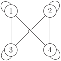
Figure 1: The complete graph with 4 nodes

From Eq. (25) and $\bm{M}\approx\bm{C}$, $m$-th moment $\mathbb{E}_{f^{(n)}_{\Lambda}\!}\bigl{[}(1-\Lambda)^{m}\bigr{]}$ is approximated by

$$\mathbb{E}_{f^{(n)}_{\Lambda}\!}\bigl{[}(1-\Lambda)^{m}\bigr{]}\approx\frac{1}{n-1}\mathbb{E}_{\mathbb{P}\left[\bm{\Gamma}\right]\!}\bigl{[}\mathrm{Tr}\!\left[\bm{C}^{m}\right]\bigr{]}.$$ (35)

As $n\rightarrow\infty$, the error of the approximation approaches to $0$. Hence, we investigate $\mathbb{E}_{\mathbb{P}\left[\bm{\Gamma}\right]\!}\bigl{[}\mathrm{Tr}\!\left[\bm{C}^{m}\right]\bigr{]}$ in order to prove that $\mathbb{E}_{f^{(n)}_{\Lambda}\!}\bigl{[}(1-\Lambda)^{m}\bigr{]}$ converges to Eqs. (21) and (22) as $n\rightarrow\infty$.

To show the convergence of even moment $\mathbb{E}_{f^{(n)}_{\Lambda}\!}\bigl{[}(1-\Lambda)^{2m}\bigr{]}$, we investigate $\mathbb{E}_{\mathbb{P}\left[\bm{\Gamma}\right]\!}\bigl{[}\mathrm{Tr}\!\left[\bm{C}^{2m}\right]\bigr{]}$. Using the independence of $C(i,j)$, even moment $\mathbb{E}_{\mathbb{P}\left[\bm{\Gamma}\right]\!}\bigl{[}\mathrm{Tr}\!\left[\bm{C}^{2m}\right]\bigr{]}$ is bounded by

$$\mathbb{E}_{\mathbb{P}\left[\bm{\Gamma}\right]\!}\bigl{[}\mathrm{Tr}\!\left[\bm{C}^{2m}\right]\bigr{]} =\sum_{\bm{v}_{m}\in\Phi_{n,2m}}\prod_{l=1}^{h(\bm{v}_{m})}\mathbb{E}_{\mathbb{P}\left[\bm{\Gamma}\right]\!}\bigl{[}C(e_{l})^{m_{l}}\bigr{]}$$

$$\leq\sum_{l=0}^{m}|Z_{l,m}| \frac{\mathbb{E}_{p_{W}\!}\bigl{[}W^{2}\bigr{]}^{l}\,\mathbb{E}_{p_{W}\!}\bigl{[}W^{2(m-l)}\bigr{]}\rho^{l}}{\mathbb{E}_{p_{W}\!}\bigl{[}W\bigr{]}^{2m}\omega_{\rm min}^{2m-2l}}\left(1+o(1)\right)$$

$$\leq\sum_{l=0}^{m}|Z_{l,m}| \frac{\mathbb{E}_{p_{W}\!}\bigl{[}W^{2}\bigr{]}^{l}\rho^{l}}{\mathbb{E}_{p_{W}\!}\bigl{[}W\bigr{]}^{2m}\omega_{\rm min}^{2m-2l}}\left(1+o(1)\right),$$ (36)

where $Z_{l,m}$ is a set of cycles $(v_{1},v_{2},...,v_{2m})$ with length $2m$ and disjoint $l+1$ nodes. Note that $Z_{l,m}\subset\Phi_{n,2m}$. For example, $(1,2,3,1,2,3)$ is included in $Z_{2,3}$. The cycles included in $Z_{l,m}$ are composed of at least $l$ disjoint links. To derive the second right-hand side of the above equation, we first divide all cycles in $\Phi_{n,2m}$ into the sets $Z_{l,m}$ of the cycles that the number of disjoint links is $l$. Each set has $|Z_{l,m}|$ cycles. Using Eq. (31), for $\bm{v}_{m}\in Z_{l,m}$, we obtain

$$\prod_{l=1}^{h(\bm{v}_{m})}\mathbb{E}_{\mathbb{P}\left[\bm{\Gamma}\right]\!}\bigl{[}C(e_{l})^{m_{l}}\bigr{]}\leq\frac{\mathbb{E}_{p_{W}\!}\bigl{[}W^{2}\bigr{]}^{l}\,\mathbb{E}_{p_{W}\!}\bigl{[}W^{2(m-l)}\bigr{]}\rho^{l}}{\mathbb{E}_{p_{W}\!}\bigl{[}W\bigr{]}^{2m}\omega_{\rm min}^{2m-2l}},$$ (37)

since that $\mathbb{E}_{p_{W}\!}\bigl{[}W^{2}\bigr{]}$ is the largest in $m$-th moments $\mathbb{E}_{p_{W}\!}\bigl{[}W^{m}\bigr{]}$ for $m\geq 2$. In the first right-hand side of Eq. (36), the reason why we do not consider the cycles longer than $m$ is as follows. First, $\mathbb{E}_{\mathbb{P}\left[\bm{\Gamma}\right]\!}\bigl{[}C(i,j)\bigr{]}=0$. Hence, $\prod_{l=1}^{h(\bm{v}_{m})}\mathbb{E}_{\mathbb{P}\left[\bm{\Gamma}\right]\!}\bigl{[}C(e_{l})^{m_{l}}\bigr{]}$ is 0 except if $m_{l}\geq 2$ for $1\leq l\leq h(\bm{v}_{m})$. Since $m_{l}\geq 2$ for $1\leq l\leq h(\bm{v}_{m})$, the number of links $l$ in the cycle is at most $m$.

To extract the main term of $\mathbb{E}_{\mathbb{P}\left[\bm{\Gamma}\right]\!}\bigl{[}\mathrm{Tr}\!\left[\bm{C}^{2m}\right]\bigr{]}$, we rewrote Eq. (36) with

$$\mathbb{E}_{\mathbb{P}\left[\bm{\Gamma}\right]\!}\bigl{[}\mathrm{Tr}\!\left[\bm{C}^{2m}\right]\bigr{]} \leq\sum_{l=1}^{m}\eta_{l,m}=\eta_{m,m}\sum_{l=1}^{m}\frac{\eta_{l,m}}{\eta_{m,m}},$$ (38)

where $\eta_{l,m}$ is

$$\eta_{l,m} =|Z_{l,m}|\frac{\mathbb{E}_{p_{W}\!}\bigl{[}W^{2}\bigr{]}^{l}\rho^{l}}{\mathbb{E}_{p_{W}\!}\bigl{[}W\bigr{]}^{2m}\omega_{\rm min}^{2m-2l}}.$$ (39)

In the above equation, $|Z_{l,m}|$ is given by

$$|Z_{l,m}| =|Z_{a}(l,m)|\,|Z_{b}(l,m)|\,|Z_{c}(l,m)|$$

$$=\frac{n!}{(n-l-1)!}\binom{2m}{2l}(l+1)^{4\,(m-l)}\frac{1}{l+1}\binom{2l}{l},$$ (40)

where $Z_{a}(l,m)$ is the number of permutations $(i_{k})_{1\leq k\leq l+1}$ by selecting $l+1$ nodes from $n$ nodes, and is given by

$$|Z_{a}(l,m)|=\frac{n!}{(n-l-1)!}.$$ (41)

Then, $|Z_{b}(l,m)|$ is the number of combinations that each $i_{k}$ appears more than once in the cycle with length $2m$, and is given by

$$|Z_{b}(l,m)|\! =\!\binom{2m}{2l}\!\!\left((l+1)^{2}\right)^{2(m-l)}\!\!=\!\binom{2m}{2l}\!\!\left(l+1\right)^{4(m-l)}.$$ (42)

In the above equation, since there is no restriction except that each $i_{k}$ must appear at least twice, it is multiplied by $\left(l+1\right)^{4(m-l)}$. Moreover, $Z_{c}(l,m)$ is the number of the second appearance positions for $i_{k}$, and is given by

$$|Z_{c}(l,m)| =\frac{1}{l+1}\binom{2l}{l}.$$ (43)

Note that the right side of the above equation is the Catalan number.

By substituting Eq. (40) into Eq. (39), $\eta_{l,m}$ is given by

$$\eta_{l,m} =|Z_{l,m}|\frac{\mathbb{E}_{p_{W}\!}\bigl{[}W^{2}\bigr{]}^{l}\rho^{l}}{\mathbb{E}_{p_{W}\!}\bigl{[}W\bigr{]}^{2m}\omega_{\rm min}^{2m-2l}}$$

$$=\frac{n!}{(n-l-1)!}\binom{2m}{2l}(l+1)^{4(m-l)}$$

$$\hskip 56.9055pt\frac{1}{l+1}\binom{2l}{l}\frac{\mathbb{E}_{p_{W}\!}\bigl{[}W^{2}\bigr{]}^{l}\rho^{l}}{\mathbb{E}_{p_{W}\!}\bigl{[}W\bigr{]}^{2m}\omega_{\rm min}^{2m-2l}}.$$ (44)

Then, $\frac{\eta_{l,m}}{\eta_{m,m}}$ in (38) is bounded by

$$\frac{\eta_{l,m}}{\eta_{m,m}} =\frac{(n-m-1)!}{(n-l-1!)}\binom{2m}{2l}(l+1)^{4(m-l)}$$

$$\hskip 28.45274pt\frac{m+1}{l+1}\frac{\binom{2l}{l}}{\binom{2m}{m}}\frac{\mathbb{E}_{p_{W}\!}\bigl{[}W^{2}\bigr{]}^{l}\mathbb{E}_{p_{W}\!}\bigl{[}W^{2m-2l}\bigr{]}\rho^{l}}{\omega_{\rm min}^{2m-2l}\mathbb{E}_{p_{W}\!}\bigl{[}W^{2}\bigr{]}^{m}\rho^{m}}$$

$$\leq\binom{2m}{2l}\frac{n^{l-m}(l+1)^{4(m-l)}4^{l-m}}{\omega_{\rm min}^{2(m-l)}\mathbb{E}_{p_{W}\!}\bigl{[}W^{2}\bigr{]}^{m-l}\rho^{m-l}}$$

$$\leq\frac{n^{l-m}\,2\,m^{2(m-l)}\,m^{4(m-l)}4^{l-m}}{\omega_{\rm min}^{2(m-l)}\mathbb{E}_{p_{W}\!}\bigl{[}W^{2}\bigr{]}^{m-l}\rho^{m-l}}$$

$$\leq 2\left[\frac{\omega_{\rm avg}\,m^{6}}{4\,\omega_{\rm min}^{2}\mathbb{E}_{p_{W}\!}\bigl{[}W^{2}\bigr{]}}\right]^{m-l}.$$ (45)

To obtain the upper bound of $\frac{\eta_{l,m}}{\eta_{m,m}}$, we used the Stirling’s approximation, which is

$$\sqrt{2\,\pi}n^{n+1/2}\,e^{-n}\leq n!\leq n^{n+1/2}\,e^{-n+1}.$$ (46)

According to the following discussion, if the degree condition is satisfied the right-hand side of Eq. (45) for $m>l$ becomes $o(1)$. First, for $m>l$, we derive

$$\left[\frac{\omega_{\rm avg}\,m^{6}}{4\,\omega_{\rm min}^{2}\mathbb{E}_{p_{W}\!}\bigl{[}W^{2}\bigr{]}}\right]^{m-l}=o(1).$$ (47)

To prove the above equation, we should show

$$\frac{\omega_{\rm avg}\,m^{6}}{4\,\omega_{\rm min}^{2}\mathbb{E}_{p_{W}\!}\bigl{[}W^{2}\bigr{]}}=o(1).$$ (48)

Similarly to [9], using $m=\log n$, we obtain condition

$$\omega_{\rm min}^{2}=\Omega((\log n)^{6})\frac{\omega_{\rm avg}}{\mathbb{E}_{p_{W}\!}\bigl{[}W^{2}\bigr{]}},$$ (49)

to satisfy Eqs. (47) and (48). The condition (49) is the same as the degree condition (16).

Therefore, if the degree condition (16) is satisfied, for $m>l$, we obtain

$$\frac{\eta_{l,m}}{\eta_{m,m}}=o(1).$$ (50)

By substituting the above equation into Eq. (38), the upper bound of $\mathbb{E}_{\mathbb{P}\left[\bm{\Gamma}\right]\!}\bigl{[}\mathrm{Tr}\!\left[\bm{C}^{2m}\right]\bigr{]}$ is given by

$$\mathbb{E}_{\mathbb{P}\left[\bm{\Gamma}\right]\!}\bigl{[}\mathrm{Tr}\!\left[\bm{C}^{2m}\right]\bigr{]}\leq\left(1+o(1)\right)\eta_{m,m}.$$ (51)

On the other hand, the lower bound of $\mathbb{E}_{\mathbb{P}\left[\bm{\Gamma}\right]\!}\bigl{[}\mathrm{Tr}\!\left[\bm{C}^{2m}\right]\bigr{]}$ is given by

$$\mathbb{E}_{\mathbb{P}\left[\bm{\Gamma}\right]\!}\bigl{[}\mathrm{Tr}\!\left[\bm{C}^{2m}\right]\bigr{]}=\sum_{\bm{v}_{m}\in\Phi_{n,m}}\prod_{h=1}^{h(\bm{v}_{m})}\mathbb{E}_{\mathbb{P}\left[\bm{\Gamma}\right]\!}\bigl{[}C(e_{l})^{m_{l}}\bigr{]}$$

$$\hskip 28.45274pt\geq|Z_{m,m}|\mathbb{E}_{\mathbb{P}\left[\bm{\Gamma}\right]\!}\bigl{[}C(i,j)^{2}\bigr{]}^{m}$$

$$\hskip 28.45274pt\geq|Z_{m,m}|\rho^{m}\frac{\mathbb{E}_{p_{W}\!}\bigl{[}W^{2}\bigr{]}^{m}}{\mathbb{E}_{p_{W}\!}\bigl{[}W\bigr{]}^{2m}}(1-o(1))$$

$$\hskip 28.45274pt=(1-o(1))\,\eta_{m,m}.$$ (52)

Note that we obtained the second right-hand side of the above equation by only using the cycles with disjoint $m$ links. To derive the third right-hand side, we used

$$\mathbb{E}_{\mathbb{P}\left[\bm{\Gamma}\right]\!}\bigl{[}C(i,j)^{2}\bigr{]}\geq\rho\frac{\mathbb{E}_{p_{W}\!}\bigl{[}W^{2}\bigr{]}}{\mathbb{E}_{p_{W}\!}\bigl{[}W\bigr{]}^{2}}(1-o(1)).$$ (53)

This can be derived from Eq. (30).

According to Eqs. (38) and (52), $\mathbb{E}_{\mathbb{P}\left[\bm{\Gamma}\right]\!}\bigl{[}\mathrm{Tr}\!\left[\bm{C}^{2m}\right]\bigr{]}$ is bounded by

$$\eta_{m,m}(1-o(1))\leq\mathbb{E}_{\mathbb{P}\left[\bm{\Gamma}\right]\!}\bigl{[}\mathrm{Tr}\!\left[\bm{C}^{2m}\right]\bigr{]}\leq\eta_{m,m}(1+o(1)).$$ (54)

As $n\rightarrow\infty$, even moment $\mathbb{E}_{f_{\Lambda}^{(n)}\!}\bigl{[}(1-\lambda)^{2m}\bigr{]}$ converges to

$$\lim_{n\rightarrow\infty}\mathbb{E}_{f_{\Lambda}^{(n)}\!}\bigl{[}(1-\lambda)^{2m}\bigr{]}=\lim_{n\rightarrow\infty}\frac{1}{n-1}\mathbb{E}_{\mathbb{P}\left[\bm{\Gamma}\right]\!}\bigl{[}\mathrm{Tr}\!\left[\bm{C}^{2m}\right]\bigr{]}$$

$$\hskip 2.84544pt=\lim_{n\rightarrow\infty}\frac{1\pm o(1)}{n-1}\eta_{m,m}$$

$$\hskip 2.84544pt=\lim_{n\rightarrow\infty}\frac{n!}{\!(n-1)(n-m-1)!}\frac{1}{m+1}\!\binom{2m}{m}\!\frac{\mathbb{E}_{p_{W}\!}\bigl{[}W^{2}\bigr{]}^{m}\!\!\rho^{m}}{\mathbb{E}_{p_{W}\!}\bigl{[}W\bigr{]}^{2m}}$$

$$\hskip 2.84544pt=\lim_{n\rightarrow\infty}g(n)\frac{\mathbb{E}_{p_{W}\!}\bigl{[}W^{2}\bigr{]}^{m}}{\omega_{\rm avg}^{m}\mathbb{E}_{p_{W}\!}\bigl{[}W\bigr{]}^{2m}}\frac{1}{m+1}\binom{2m}{m}$$

$$\hskip 2.84544pt=\frac{\mathbb{E}_{p_{W}\!}\bigl{[}W^{2}\bigr{]}^{m}}{\omega_{\rm avg}^{m}\mathbb{E}_{p_{W}\!}\bigl{[}W\bigr{]}^{2m}}\frac{1}{m+1}\binom{2m}{m}$$

$$\hskip 2.84544pt=\left(\frac{\tilde{r}}{2}\right)^{2m}\frac{(2\,m)!}{m!\,(m+1)!},$$ (55)

where $g(n)$ is defined by

$$g(n):=\frac{n!}{(n\!-\!1)(n\!-\!m\!-\!1)!\,n^{m}}.$$ (56)

Note that $\lim_{n\rightarrow\infty}g(n)=1$.

Therefore, if weighted network $G$ satisfies the degree condition (16), even moment $\mathbb{E}_{\mathbb{P}\left[\bm{\Gamma}\right]\!}\bigl{[}\mathrm{Tr}\!\left[\bm{C}^{2m}\right]\bigr{]}$ converges to $\mathbb{E}_{\tilde{f}_{\Lambda}\!}\bigl{[}(1-\lambda)^{2m}\bigr{]}$ as $n\rightarrow\infty$.

Next, we investigate odd moment $\mathbb{E}_{\mathbb{P}\left[\bm{\Gamma}\right]\!}\bigl{[}\mathrm{Tr}\!\left[\bm{C}^{2m+1}\right]\bigr{]}$. Similarly to even moment $\mathbb{E}_{\mathbb{P}\left[\bm{\Gamma}\right]\!}\bigl{[}\mathrm{Tr}\!\left[\bm{C}^{2m}\right]\bigr{]}$, $\mathbb{E}_{\mathbb{P}\left[\bm{\Gamma}\right]\!}\bigl{[}\mathrm{Tr}\!\left[\bm{C}^{2m+1}\right]\bigr{]}$ is bounded by

$$\mathbb{E}_{\mathbb{P}\left[\bm{\Gamma}\right]\!}\bigl{[}\mathrm{Tr}\!\left[\bm{C}^{2m+1}\right]\bigr{]} =\sum_{\bm{v}_{m}\in\Phi_{n,2m+1}}\prod_{l=1}^{h(\bm{v}_{m})}\mathbb{E}_{\mathbb{P}\left[\bm{\Gamma}\right]\!}\bigl{[}C(e_{l})^{m_{l}}\bigr{]}$$

$$\leq\sum_{l=0}^{m}|Z_{l,m}| \frac{\mathbb{E}_{p_{W}\!}\bigl{[}W^{2}\bigr{]}^{l-1}\rho^{l}}{\mathbb{E}_{p_{W}\!}\bigl{[}W\bigr{]}^{2m+1}\omega_{\rm min}^{2m-2l+1}}\left(1+o(1)\right)$$

$$\leq\sum_{l=0}^{m}\frac{\eta_{l,m}^{\prime}}{\omega_{\rm min}} =\frac{\eta_{m,m}^{\prime}}{\omega_{\rm min}}\sum_{l=0}^{m}\left(\frac{\eta_{l,m}^{\prime}}{\eta_{m,m}^{\prime}}\right),$$ (57)

where $\sum_{h=1}^{l}m_{h}=2m+1$, and $\eta_{l,m}^{\prime}$ is given by

$$\eta_{l,m}^{\prime}=|Z_{l,m}| \frac{\mathbb{E}_{p_{W}\!}\bigl{[}W^{2}\bigr{]}^{l-1}\rho^{l}}{\mathbb{E}_{p_{W}\!}\bigl{[}W\bigr{]}^{2m+1}\omega_{\rm min}^{2m-2l}}\left(1+o(1)\right).$$ (58)

Using the similar way of the even moment, $\eta_{l,m}^{\prime}/\eta_{m,m}^{\prime}$ is bounded by

$$\frac{\eta_{l,m}^{\prime}}{\eta_{m,m}^{\prime}} \leq 2\left[\frac{\omega_{\rm avg}\,m^{6}}{4\,\omega_{\rm min}^{2}\mathbb{E}_{p_{W}\!}\bigl{[}W^{2}\bigr{]}}\right]^{m-l}.$$ (59)

If the degree condition (16) is satisfied, for $m>l$, we obtain

$$\left[\frac{\omega_{\rm avg}\,m^{6}}{4\,\omega_{\rm min}^{2}}\right]^{m-l}=o(1).$$ (60)

Hence, the upper bound of $1/(n-1)\mathbb{E}_{\mathbb{P}\left[\bm{\Gamma}\right]\!}\bigl{[}\mathrm{Tr}\!\left[\bm{C}^{2m+1}\right]\bigr{]}$ is given by

$$\frac{1}{n-1}\mathbb{E}_{\mathbb{P}\left[\bm{\Gamma}\right]\!}\bigl{[}\mathrm{Tr}\!\left[\bm{C}^{2m+1}\right]\bigr{]}\leq\frac{1+o(1)}{n-1}\frac{\eta_{m,m}^{\prime}}{\omega_{\rm min}}.$$ (61)

As $n\rightarrow\infty$, the right-hand side of the above equation converges to

$$\lim_{n\rightarrow\infty}\frac{1+o(1)}{n-1}\frac{\eta_{m,m}^{\prime}}{\omega_{\rm min}}$$

$$\hskip 2.84544pt=\lim_{n\rightarrow\infty}\frac{g(n)}{m+1}\!\binom{2m}{m}\!\frac{\mathbb{E}_{p_{W}\!}\bigl{[}W^{2}\bigr{]}^{m-1}}{\mathbb{E}_{p_{W}\!}\bigl{[}W\bigr{]}^{2m+1}\omega_{\rm avg}^{m}\omega_{\rm min}}$$

$$\hskip 2.84544pt=\left(\frac{\tilde{r}}{2}\right)^{2m}\!\!\!\frac{(2\,m)!}{m!\,(m+1)!}\lim_{n\rightarrow\infty}\frac{g(n)}{\mathbb{E}_{p_{W}\!}\bigl{[}W^{2}\bigr{]}\mathbb{E}_{p_{W}\!}\bigl{[}W\bigr{]}\omega_{\rm min}}$$

$$\hskip 2.84544pt=0.$$ (62)

Note that $1/\omega_{\rm min}=o(1)$ since $\omega_{\rm min}$ is a increasing function of $n$. Hence, as $n\rightarrow\infty$, odd moment $\mathbb{E}_{f^{(n)}_{\Lambda}\!}\bigl{[}(1-\Lambda)^{2m+1}\bigr{]}$ is given by

$$\lim_{n\rightarrow\infty}\mathbb{E}_{f^{(n)}_{\Lambda}\!}\bigl{[}(1-\Lambda)^{2m+1}\bigr{]} =\lim_{n\rightarrow\infty}\frac{(1+o(1))}{n-1}\frac{\eta_{m,m}^{\prime}}{\omega_{\rm min}}$$

$$=0.$$ (63)

Therefore, if weighted network $G$ satisfies the degree condition (16), odd moment also converges to $\mathbb{E}_{\tilde{f}_{\Lambda}\!}\bigl{[}(1-\Lambda)^{2m+1}\bigr{]}$ as as $n\rightarrow\infty$. ∎

4 Numerical Example

We confirm the the validity of the degree condition (16) and Eq. (20) in the Wigner’s semicircle law for weighted network $G$ derived in Sect. 3. For the sake of space, we only show the results using the BA model [10], which is a famous random network generation model.

Similarly to [6], we generate weighted network $G$ with the following procedures based on the BA model.

1. Generate an unweighted network with $n$ nodes and average degree $\omega_{\rm avg}^{\rm BA}$ according to the BA model.

2. Randomly cut the links of the unweighted network until the average degree is $\omega_{\rm avg}$. This procedure prevents minimum degree $\omega_{\rm min}$ from being fixed, and does not lose the scale-free property of the BA network [6].

3. Randomly assign the weight of each link using the Pareto distribution $p_{W}^{\rm par}(w)$ with $\mathbb{E}_{p_{W}\!}\bigl{[}W\bigr{]}=1$. Note that $p_{W}^{\rm par}(w)\propto\alpha\,w^{-\alpha-1}$.

4. Divide the weight of each link by maximum link weight $w_{\rm max}$. By performing this procedure, the link weight is smaller than or equal to $1$, and its distribution satisfies the condition of $p_{W}(w)$ used in Section 3. Note that this procedure does not change normalized Laplacian matrix $\bm{N}$.

In order to confirm the validity of the degree condition (16) in the Wigner’s semicircle law for weighted network $G$, we compare eigenvalue density $f_{\Lambda}^{(n)}(\lambda)$ of the normalized Laplacian matrix $\bm{N}$ and semicircle distribution $\tilde{f}_{\Lambda}(\lambda)$. To evaluate the difference of them, we use the relative error $\epsilon_{\rm d}$, which is defined by

$$\epsilon_{\rm d}:=\frac{1}{n_{h}}\sum_{i=1}^{n_{h}}\frac{|F_{n}(\theta_{i})-F^{*}(\theta_{i})|}{F(\theta_{i})},$$ (64)

where $\theta_{i}=(i-1/2)h_{b}+\lambda_{2}$ and $h_{b}=(\lambda_{n}-\lambda_{2})/n_{h}$. In (64), $F_{n}(\theta_{i})$ is the value obtained with dividing the number of eigenvalues of $\bm{N}$ within $[\theta_{i}-h_{b}/2,\theta_{i}+h_{b}/2]$ by $n-1$. On the contrary, $F^{*}(\theta_{i})$ is the value of the integral of $\tilde{f}_{\Lambda}(\lambda)$ within $[\theta_{i}-h_{b}/2,\theta_{i}+h_{b}/2]$.

In order to confirm the validity of Eq. (20), we compare spectral radius $r$ of normalized Laplacian matrix $\bm{N}$ and $\tilde{r}$ calculated by Eq. (20). For these comparisons, we use relative error $\epsilon_{r}$, which is defined by

$$\epsilon_{r}:=\frac{|\tilde{r}-r|}{r}.$$ (65)

In the numerical example, we use the parameter configuration shown in Tab. 1 as a default parameter configuration.

Table 1: Parameter configuration

Average degree of unweighted BA networks, $\omega_{\rm avg}^{(BA)}$	40
Number of nodes of weighted network $G$, $n$	1,000
Average degree of weighted network $G$, $\omega_{\rm avg}$	20
Pareto index of the Pareto distribution, $\alpha$	3
Number of bins, $n_{h}$	50

First, we confirm the relationship between the characteristics of weighted network $G$ generated in the above procedure and the degree condition (16). Figure 2 shows the square of the minimum degree, $\omega_{\rm min}^{2}$ for different average degree $\omega_{\rm avg}$. In this figure, we also plots the results with the average order $\omega_{\rm avg}$ on the $y$ axis for comparison. From these results, as $\omega_{\rm avg}$ increases, the difference between $\omega_{\rm min}^{2}$ and $\omega_{\rm avg}$ increases, and hence the degree condition (16) is more easily satisfied. Figure 3 shows second moment $\mathbb{E}_{p_{W}\!}\bigl{[}W^{2}\bigr{]}$ of link weights for different Pareto index $\alpha$. From this figure, as $\alpha$ increases, $\mathbb{E}_{p_{W}\!}\bigl{[}W^{2}\bigr{]}$ increases, and hence the degree condition (16) is also more easily satisfied.

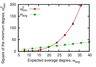
Figure 2: Average degree $\omega_{\rm avg}$ vs. the square of the minimum degree, $\omega_{\rm min}^{2}$

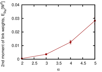
Figure 3: Second moment $\mathbb{E}_{p_{W}\!}\bigl{[}W^{2}\bigr{]}$ for different Pareto index $\alpha$

Figures 4 (a) and (b) show eigenvalue density $f_{\Lambda}^{(n)}(\lambda)$ of the normalized Laplacian matrix $\bm{N}$ (i.e, $F_{n}(\theta)$) and semicircle distribution $\tilde{f}_{\Lambda}(\lambda)$. For reference, we show the results of all link weights $w(i,j)=1$ in Fig. 4 (c). According to the results, eigenvalue density $f_{\Lambda}^{(n)}(\lambda)$ for $\alpha=5$ is closer to semicircle distribution $\tilde{f}_{\Lambda}(\lambda)$ than that for $\alpha=3$. This is consistent with the result of $\mathbb{E}_{p_{W}\!}\bigl{[}W^{2}\bigr{]}$ shown in Fig. 3. Hence, we visually confirm the validity of the degree condition (16).

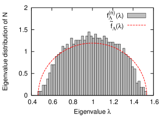
(a) pareto distribution with $\alpha=3$

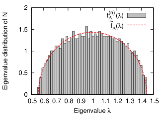
(b) pareto distribution with $\alpha=5$

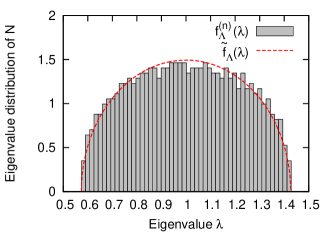
(c) $w(i,j)=1$

Figure 4: Eigenvalue density $f_{\Lambda}^{(n)}(\lambda)$ of the normalized Laplacian matrix $\bm{N}$ (i.e, $F_{n}(\theta)$) and semicircle distribution $\tilde{f}_{\Lambda}(\lambda)$

Figure 5 shows relative error $\epsilon_{\rm d}$ of eigenvalue density $f_{\Lambda}^{(n)}(\lambda)$ for different average degree $\omega_{\rm avg}$. In this figure, we also show the result for all link weights $w(i,j)=1$ for reference. Since $n$ is finite, relative error $\epsilon_{\rm d}$ is not $0$. We assume that relative error $\epsilon_{\rm d}$ is almost equal to the result for $w(i,j)=1$, $f_{\Lambda}^{(n)}(\lambda)$ converges to $\tilde{f}_{\Lambda}(\lambda)$ as $n\rightarrow\infty$. From the results in Fig. 5, relative error $\epsilon_{\rm d}$ decreases as average degree $\omega_{\rm avg}$ increases or Pareto index $\alpha$ increases. The result is consistent with the results shown in Figs. 2 and 3. Hence, the degree condition (16) is valid. Moreover, relative error $\epsilon_{\rm d}$ for $\alpha=5$ is almost same as the that for $w(i,j)=1$. Hence, if $\alpha\geq 5$, $f_{\Lambda}^{(n)}(\lambda)$ follows the Wigner’s semicircle law.

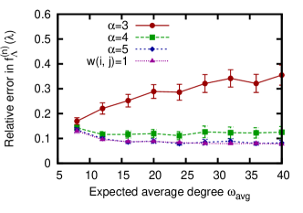
Figure 5: Relative error $\epsilon_{\rm d}$ of eigenvalue density $f_{\Lambda}^{(n)}(\lambda)$ for different average degree $\omega_{\rm avg}$

Figure 6 shows spectral radius $r$ and $\tilde{r}$ calculated from Eq. (20) for different average degree $\omega_{\rm avg}$. In this figure, we also plot the result for all link weights $w(i,j)=1$ for reference. From Fig. 6, spectral radius $r$ almost coincides with $\tilde{r}$ except for $\alpha=3$. Hence, spectral radius $r$ can be calculated accurately using Eq. (20) if the degree condition (16) is satisfied.

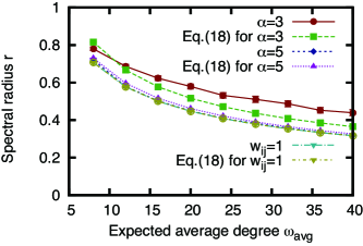
Figure 6: Spectral radius $r$ and $\tilde{r}$ calculated from Eq. (20) for different average degree $\omega_{\rm avg}$

Figure 7 shows relative error $\epsilon_{r}$ of $\tilde{r}$ calculated by Eq. (20) for different average degree $\omega_{\rm avg}$. In this figure, the result of for all link weights $w(i,j)=1$ is also plotted for reference. According to Fig. 7, it is clear that relative error $\epsilon_{r}$ is small when the degree condition (16) is easily satisfied as with the result shown in Fig. 5. Hence, Eq. (20) is valid as the approximate expression of spectral radius $r$.

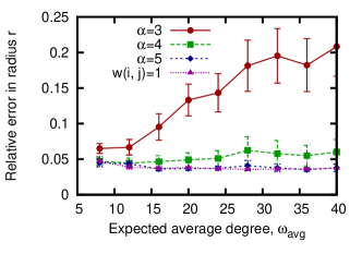
Figure 7: Relative error $\epsilon_{r}$ of $\tilde{r}$ calculated by Eq. (20) for different average degree $\omega_{\rm avg}$

From the above results, we conclude that the degree condition (16) and Eq. (20) derived in Sect. 3 are valid.

5 Conclusion and Future Work

In this paper, we have clarified the Wigner’s semicircle law for weighted network $G$ on the basis of the random matrix theory. This law indicates that if $G$ with $n$ nodes satisfies the degree condition (16), the eigenvalue density of the normalized Laplacian matrix $\bm{N}$ converges to the semicircle distribution determined by the approximated spectral radius $\tilde{r}$ as $n\rightarrow\infty$. By using Eq. (20), we can calculate $\tilde{r}$ from a few network statistics (the average degree, the average link weight, and the square average link weight). Hence, the eigenvalue distribution of $\bm{N}$ can be obtained from these network statistics without giving all matrix elements $N(i,j)$ accurately. Our results provide a new analysis method for weighted network $G$ using the spectral graph theory and the random graph theory.

As future work, we are planing to analyze and design actual networks using the Wigner’s semicircle law clarified in this paper. In particular, we will investigate the characteristics of the information dissemination on the social network, and design the social media to control the speed of the information dissemination.

Yusuke Sakumoto received M.E. and Ph.D. degrees in the Information and Computer Sciences from Osaka University in 2008 and 2010, respectively. From 2010 to 2019, he was a associate professor of Tokyo Metropolitan University. He is currently an associate professor at Kwansei Gakuin University. His research work is in the area of communication network, electricity network, and social network. He is a member of the IEEE, IEICE and IPSJ.

Masaki Aida received his B.S. degree in Physics and M.S. degree in Atomic Physics from St. Paul’s University, Tokyo, Japan, in 1987 and 1989, respectively, and his Ph.D. in Telecommunications Engineering from the University of Tokyo, Japan, in 1999. In April 1989, he joined NTT Laboratories. From April 2005 to March 2007, he was an Associate Professor at Tokyo Metropolitan University. He has been a Professor of the Graduate School of Systems Design, Tokyo Metropolitan University since April 2007. His current interests include analysis of social network dynamics and distributed control of computer communication networks. He received the Best Tutorial Paper Award and the Best Paper Award of IEICE Communications Society in 2013 and 2016, respectively, and IEICE 100-Year Memorial Paper Award in 2017. He is a fellow of IEICE and a member of the IEEE, ACM and ORSJ.

References

- [1] C. Shi, Y. Li, J. Zhang, Y. Sun, and S. Y. Philip, “A survey of heterogeneous information network analysis,” IEEE Transactions on Knowledge and Data Engineering, vol. 29, no. 1, pp. 17–37, Aug. 2016.
- [2] J. Feng, X. Li, B. Mao, Q. Xu, and Y. Bai, “Weighted complex network analysis of the Beijing subway system: Train and passenger flows,” Physica A: Statistical Mechanics and its Applications, vol. 474, pp. 213–223, Jan. 2017.
- [3] X. Sun, V. Gollnick, and S. Wandelt, “Robustness analysis metrics for worldwide airport network: A comprehensive study,” Chinese Journal of Aeronautics, vol. 30, no. 2, pp. 500–512, Feb. 2017.
- [4] F. R. Chung and F. C. Graham, Spectral graph theory. American Mathematical Soc., May 1997, no. 92.
- [5] D. A. Spielman, “Spectral graph theory and its applications,” in Proceedings of the 48th Annual IEEE Symposium on Foundations of Computer Science (FOCS’07). IEEE, Oct. 2007, pp. 29–38.
- [6] Y. Sakumoto, T. Kameyama, C. Takano, and M. Aida, “Information propagation analysis of social network using the universality of random matrix,” IEICE Transactions on Communications, vol. E102-B, no. 2, pp. 391–399, Feb. 2019.
- [7] E. P. Wigner, “On the distribution of the roots of certain symmetric matrices,” Annals of Mathematics, vol. 67, no. 2, pp. 325–327, 1958. [Online]. Available: http://www.jstor.org/stable/1970008
- [8] V. Plerou, P. Gopikrishnan, B. Rosenow, L. A. N. Amaral, T. Guhr, and H. E. Stanley, “Random matrix approach to cross correlations in financial data,” Phycal Review E, vol. 65, p. 066126, Jun. 2002. [Online]. Available: https://link.aps.org/doi/10.1103/PhysRevE.65.066126
- [9] F. Chung, L. Lu, and V. Vu, “Spectra of random graphs with given expected degrees,” the National Academy of Sciences, vol. 100, no. 11, pp. 6313–6318, Feb. 2003.
- [10] A. L. Bárabasi and R. Albert, “Emergence of scaling in random networks,” Science, vol. 286, no. 5439, pp. 509–512, Oct. 1999.