Axisymmetric Radiative Transfer Models of Kilonovae

Abstract

The detailed observations of GW170817 proved for the first time directly that neutron star mergers are a major production site of heavy elements. The observations could be fit by a number of simulations that qualitatively agree, but can quantitatively differ (e.g. in total r-process mass) by an order of magnitude. We categorize kilonova ejecta into several typical morphologies motivated by numerical simulations, and apply a radiative transfer Monte Carlo code to study how the geometric distribution of the ejecta shapes the emitted radiation. We find major impacts on both spectra and light curves. The peak bolometric luminosity can vary by two orders of magnitude and the timing of its peak by a factor of five. These findings provide the crucial implication that the ejecta masses inferred from observations around the peak brightness are uncertain by at least an order of magnitude. Mixed two-component models with lanthanide-rich ejecta are particularly sensitive to geometric distribution. A subset of mixed models shows very strong viewing angle dependence due to lanthanide “curtaining,” which persists even if the relative mass of lanthanide-rich component is small. The angular dependence is weak in the rest of our models, but different geometric combinations of the two components lead to a highly diverse set of light curves. We identify geometry-dependent P Cygni features in late spectra that directly map out strong lines in the simulated opacity of neodymium, which can help to constrain the ejecta geometry and to directly probe the r-process abundances.

1 Introduction

The origin of the rapid neutron capture (r-process) elements is one of the longest-standing unsolved problems in nuclear astrophysics with the most popular candidate sites being stellar collapse and compact object mergers (Cowan et al., 2019). Neutron star mergers have long been argued to be sources of r-process elements (Lattimer & Schramm, 1974; Eichler et al., 1989; Rosswog et al., 1998, 1999; Freiburghaus et al., 1999), mostly because their neutron richness effortlessly leads to the production of platinum-peak elements; this has been a major challenge for other production sites. Such rare events (compared to supernovae) that eject large amounts of r-process per occurrence are also supported by geological evidence (Hotokezaka et al., 2015; Wallner et al., 2015). However, without direct observational evidence, our understanding of the enrichment of the universe by r-process elements was primarily based on theoretical models (for a review, see Côté et al., 2017).

This situation changed dramatically with the gravitational and electromagnetic wave detection of a nearby neutron star merger, GW170817 (Abbott et al., 2017b). The optical and infrared emission from this merger (Chornock et al., 2017; Cowperthwaite et al., 2017; Kasliwal et al., 2017a; Kilpatrick et al., 2017; McCully et al., 2017; Rosswog et al., 2018; Smartt et al., 2017; Tanvir et al., 2017; Troja et al., 2017; Villar et al., 2017) matches theoretical expectations that much of the ejecta is r-process material (Lattimer & Schramm, 1974; Eichler et al., 1989; Rosswog et al., 1998, 1999; Freiburghaus et al., 1999; Goriely et al., 2011; Roberts et al., 2011; Korobkin et al., 2012; Wanajo et al., 2014).

The high r-process yields estimated from GW170817 combined with the large merger rate predicted by its detection (Abbott et al., 2017a), indicate that neutron star mergers could be the dominant site for galactic r-process elements (Côté et al., 2018; Rosswog et al., 2018) and, in fact, could actually produce more r-process than is observed. Current chemical evolution models (Côté et al., 2019; Wehmeyer et al., 2019), however, argue that an additional component is needed, at least at early times, to find satisfactory agreement with the observed r-process abundances.

In a supernova context, it has been known for a long time that inferring masses from the optical emission is difficult and that a given light curve can be matched by a wide range of ejecta masses (see De La Rosa et al., 2017, for example). Differences in the modeling methods (e.g. opacity implementations, transport schemes) and the applied microphysics (e.g. opacities, shock physics, equilibrium assumptions) both contribute to these errors. The situation is similar for GW170817, where a range of masses has been inferred by different groups (Côté et al., 2018; Ji et al., 2019). To better observationally constrain neutron star merger yields, kilonova emission models need to be refined, with a particular emphasis on exploring what role the ejecta geometry plays in shaping the electromagnetic emission. This is the subject that we address here.

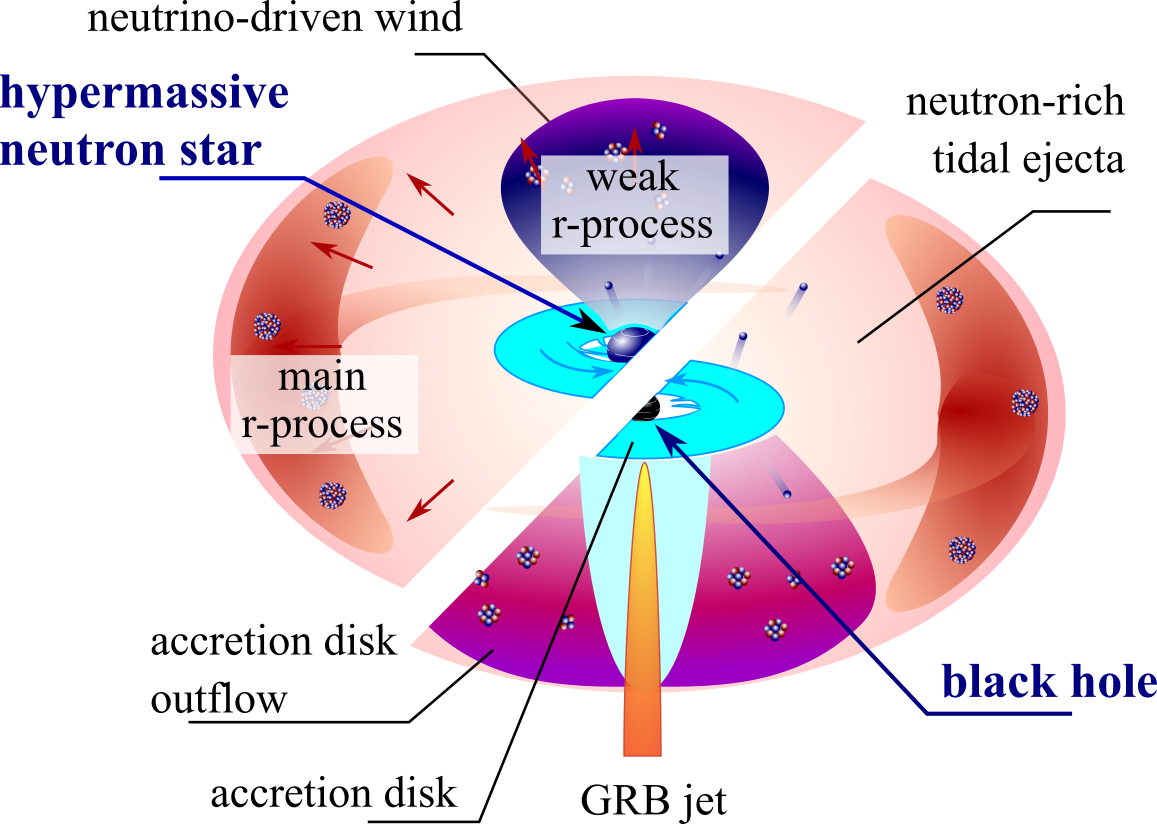
Figure 1: Sketch of the standard kilonova scenario, involving either a hypermassive neutron star (upper left) or a black hole as (lower right) a central object. Various types of ejected matter are depicted, contributing to the main and weak r-process production (see, e.g. Shibata & Hotokezaka, 2019, for a review on mass ejection in NSMs).

Recent studies (Bauswein et al., 2013; Fernández & Metzger, 2013; Rosswog et al., 2014; Just et al., 2015; Fernández et al., 2015; Radice et al., 2016; Sekiguchi et al., 2016; Baiotti & Rezzolla, 2017; Rosswog et al., 2017; Shibata et al., 2017; Fahlman & Fernández, 2018; Metzger et al., 2018; Papenfort et al., 2018; Siegel & Metzger, 2018; Radice et al., 2018; Miller et al., 2019; Krüger & Foucart, 2020) have revealed different ejecta channels and morphologies. These sources include tidal tails with low electron fractions ($Y_{e}<0.2$), polar shocked material (sometimes referred to as squeeze ejecta), magnetar or neutrino-driven wind ejecta (all with $Y_{e}\sim 0.25-0.45$) and disk wind material with electron fractions ranging from $0.1$ to $0.4$ (Metzger, 2019). A number of models have invoked two (Evans et al., 2017; Tanaka et al., 2017; Tanvir et al., 2017; Troja et al., 2017; Kawaguchi et al., 2018) or even three (Cowperthwaite et al., 2017; Perego et al., 2017; Villar et al., 2017) ejecta components to explain the electromagnetic observation of GW170817. A typical kilonova scenario with multicomponent ejecta mechanisms is sketched in Figure 1. The components may include toroidal tidally expelled highly neutron-rich ejecta, which produces the red (near-IR; nIR-IR) emission in the kilonova, or a medium neutron-rich wind emerging from the surface of a transient hypermassive neutron star and/or an accretion disk (see Shibata & Hotokezaka, 2019, for a review on mass ejection in kilonovae).

It appears that the models ignoring the multidimensional character of kilonova ejecta tend to infer higher ejected masses than multidimensional models. On the other hand, the models with a true multidimensional treatment of radiative transfer (Tanvir et al., 2017; Troja et al., 2017; Kawaguchi et al., 2018) seem to favor lighter and faster neutron-rich ejecta accompanied by a heavy “wind” with moderately neutron-rich composition (shown in Fig. 4 of Ji et al., 2019). This scenario is also supported by numerical simulations (e.g. Perego et al., 2014; Radice et al., 2016; Dietrich et al., 2017; Shibata & Hotokezaka, 2019).

The neutron-rich dynamical ejecta, or the neutron-rich outflows from the post-merger accretion disk (Janiuk, 2014; Miller et al., 2019) are expected to contain a large fraction of high-opacity lanthanides (Barnes & Kasen, 2013; Tanaka & Hotokezaka, 2013; Fontes et al., 2015; Gaigalas et al., 2019; Fontes et al., 2020). The properties of this lanthanide-rich outflow dictate how much light in optical and red bands will be blocked; in some cases, lanthanide-rich geometric configurations can produce an effective lanthanide “curtain” (Kasen et al., 2015; Wollaeger et al., 2018; Nativi et al., 2020). In such cases, the kilonova can be highly sensitive to the viewing angle.

Kilonova light curves and spectra are influenced by both ejecta morphology and microphysics, for example complicated, wavelength-dependent opacities (Kasen et al., 2017; Even et al., 2020), nuclear heating (Lippuner & Roberts, 2015), and thermalization (Barnes et al., 2016; Rosswog et al., 2017; Hotokezaka & Nakar, 2019). Opacities, nuclear heating, and thermalization are all sensitive to the density, which is specified by geometric distribution of mass. As we shall see, deviations from the spherical shape are responsible for modified light curves not only via modified surface area or “curtaining,” but mainly through an indirect effect on the microphysics because of their different density.

Previously, Kasen et al. (2017) studied different ejecta geometries: one with a light r-process composition focused around the axis to represent wind, and one with a heavy r-process composition and oblate ellipsoidal morphology to represent dynamical ejecta. In these models, the dynamical ejecta with an ellipsoid axis aspect ratio of four produces the angular variation on the order of a factor of two. In the wind ejecta, when focused into $\sim$45^∘ conical regions about the axis, Kasen et al. (2017) find an angular variation of $\sim$20% in peak luminosity. The relatively minor angular variation in peak luminosity of the wind is a result of the less extreme variation in the projected surface area of the wind, relative to the dynamical ejecta, so that the high lanthanide opacity of the low-electron-fraction ejecta played a diminished role.

In several recent works (Barbieri et al., 2019; Darbha & Kasen, 2020; Zhu et al., 2020), sensitivity of the light curves to inclination angle was investigated using uniform gray opacity with a variety of nonspherical 2D and 3D analytically prescribed shapes. The resulting light curves exhibit only mild variability, within a factor of $\sim$2-3, because the projected area of the photosphere, which serves as a proxy for angular dependence, does not vary substantially. However, the location of the photosphere itself, and more importantly, its temperature, strongly depend on the properties of material-specific opacities. Here we explore the differences between detailed and gray-opacity prescription and conclude that more realistic detailed opacity enhances morphological variability in the light curves beyond the projected-area effects.

In Bulla (2019), it was demonstrated that a multidimensional two-component model deviates strongly from a simple sum of single-component ones. However, bound–bound opacities were approximated using a time-dependent analytic fit. This excludes temperature feedback on the opacity, which is also substantial, as we show here. Kawaguchi et al. (2020) performed advanced special-relativistic radiative transfer simulations of axisymmetric two-component models of kilonova from dynamical ejecta with morphology fits to numerical relativity (Kiuchi et al., 2017; Hotokezaka et al., 2018) and spherical post-merger outflows. They used a full suite of line r-process opacities (Tanaka et al., 2020) and found several strong effects of multidimensional, multicomponent interaction, such as preferential diffusion toward polar regions in the presence of toroidal optically thick dynamical ejecta and significant dependence on inclination angle due to the “lanthanide curtaining.” We describe similar effects observed in our models, but also take a broader set of possible morphologies and compare the light curves to gray-opacity models in order to understand their limitations.

In this paper, we study the importance of morphology in combination with its effects on microphysics, focusing on the geometrical distributions that depart from spherical symmetry. Ejecta morphologies are generated from the family of Cassini ovals in 2D axisymmetric geometry. For these morphologies, we demonstrate the enhancement to the radiative flux when departing from spherical symmetry. We then proceed to construct two-component models, representing different possible configurations of low-electron-fraction ($Y_{e}$) dynamical ejecta/accretion disk outflows, and high-$Y_{e}$ wind. For each of the components, we employ a respective composition and nuclear heating representative of low-$Y_{e}$ or high-$Y_{e}$ post-nucleosynthetic conditions. Here we demonstrate the following effects of radiative interaction between two superimposed components: lanthanide curtaining, photon reprocessing, and photon redirection. Our other recent work provides preliminary studies focusing specifically on the effects of composition (Even et al., 2020) and additional energy sources (Wollaeger et al., 2019).

This paper is organized as follows. In Section 2, we discuss the numerical methods and approximations made in our simulations. In Section 2.3, we describe the functional forms and compositions of our model ejecta. In Section 3, we present light curves and spectra for several of our one- and two-component models, and discuss the effect of morphology and superimposing of the components on these observables. We conclude in Section 4 with a summary of the results and discussion of the possible impact of morphology on the interpretation of observations. In Appendix A, we provide absolute AB magnitudes for each model, in the $r$ and $J$ bands at days 1, 4, and 8. In Appendix B, we give a detailed analysis of the radiative structure of single-component axisymmetric morphologies and different factors affecting their electromagnetic emission.

2 Methods

In this section, we review our approach for modeling kilonovae, which involves computing multiwavelength opacity tables and using them to simulate radiative transfer through homologously expanding ejecta. Our code uses the same method and opacity implementation as described in Wollaeger et al. (2018, 2019), Even et al. (2020), and Fontes et al. (2020). Below we briefly review this methodology and then focus primarily on the improvements to the opacity and radiative transfer introduced for this paper.

2.1 Radiative transfer modeling

We employ the multidimensional Monte Carlo radiative transfer software SuperNu (Wollaeger & van Rossum, 2014) to synthesize the spectra from our models. SuperNu uses a Monte Carlo method for thermal radiative transfer that is semi-implicit in time, which introduces an effective scattering term (Fleck Jr & Cummings Jr, 1971). A discrete diffusion Monte Carlo (DDMC) optimization is also implemented to replace multiple small scattering steps with larger jumps between spatial cells (Abdikamalov et al., 2012; Densmore et al., 2012; Cleveland & Gentile, 2014). DDMC has recently been generalized to include leakage probabilities out of lines for Lyman-$\alpha$ transport (Smith et al., 2018). The geometries available are spherical, axisymmetric, and Cartesian, each in 1D, 2D, or 3D. In the calculations presented here, we have incorporated an improved treatment of Doppler shift in DDMC (R. T. Wollaeger et al 2020, in preparation), that is consistent with the opacity-regrouping algorithm described by Wollaeger & van Rossum (2014). This Doppler shift algorithm has permitted more accurate application of DDMC on the binned opacities described by Fontes et al. (2020).

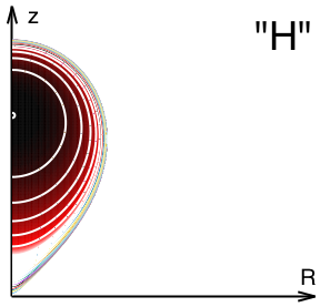
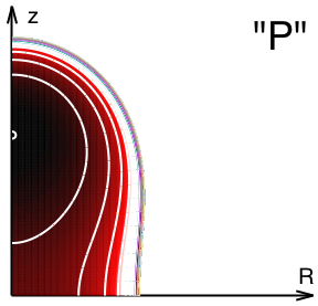
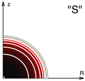
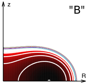
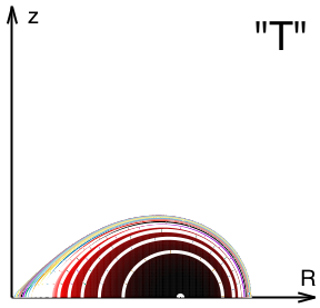
Figure 2: Maps of density of the basic building-block morphologies used in this work, shown in the upper polar half-plane (the $R-z$ plane, with $R$ being the cylindrical radius): "hourglass" (H), "peanut" (P), "sphere" (S), "biconcave" (B), and "torus" (T). The contours are equi-spaced by 0.5 dex in log space, down from the density maximum.

Originally intended for supernova transients (van Rossum et al., 2016; Kozyreva et al., 2017; Wollaeger et al., 2017), SuperNu has been applied to modeling kilonovae in 1D and 2D axisymmetric geometry (Evans et al., 2017; Kasliwal et al., 2017b; Tanvir et al., 2017; Troja et al., 2017; Wollaeger et al., 2018, 2019; Even et al., 2020). These studies varied the mass and velocity of wind and dynamical ejecta components but always assumed a spherical wind superimposed with ejecta from SPH simulations (Rosswog et al., 2014). The morphologies we explore in this paper more systematically test the multidimensional functionality of SuperNu.

2.2 Choice of composition and opacities

We use tabulated opacities generated with the LANL suite of atomic physics codes (Fontes et al., 2015). As with Fontes et al. (2017) and Wollaeger et al. (2018), the tables are calculated under the assumption of local thermodynamic equilibrium (LTE), where ionization and excitation populations can be obtained from Saha–Boltzmann statistics. For this work, we use an updated approach to the tabulation of opacity, which employs the binning of lines instead of smearing them over multiple wavelength points (Fontes et al., 2020). In conjunction with the higher group resolution in SuperNu  this approach permits more resolved spectra for lower-velocity outflows. For the radiative transfer, the frequency values for each density and temperature point of these tables are mapped to a logarithmic 1024-group wavelength grid from $10^{3}$ to $1.28\times 10^{5}$ Å.

All models in this study use one of the two compositions, representing a low- and high-electron-fraction ($Y_{e}$) abundance pattern. The low-$Y_{e}$ abundance pattern follows the solar r-process residuals and is the same as that in Even et al. (2020), their Fig. 1(b). It includes all lanthanides, uranium representing the actinides, and lighter r-process elements represented by Se, Br, Te, Pd, Zr, and Fe. The high-$Y_{e}$ abundance pattern is the “wind 2” composition studied in (Wollaeger et al., 2018, see their Fig. 3). Throughout this paper, we will refer to these two cases as “low-$Y_{e}$” and “high-$Y_{e}$” compositions. Sometimes, for simplicity, we refer to these components as “dynamical ejecta” and “wind,” respectively, but in general, low-$Y_{e}$ material does not necessarily come from the dynamical ejection (Fernández & Metzger, 2013), while high-$Y_{e}$ material does not have to be generated in the wind (Wanajo et al., 2014).

Nuclear composition influences the amount and type of radioactive nuclear heating produced in the ejecta over time (Lippuner & Roberts, 2015; Zhu et al., 2018, 2019). We use detailed time-dependent nuclear heating output from a nucleosynthesis network which calculates separate contributions from different types of radiation ($\alpha$-, $\beta$-, $\gamma$-radiation, and fission fragments) and their thermalization. The latter is estimated using phenomenological formulae from Barnes et al. (2016) (as in Rosswog et al., 2017; Wollaeger et al., 2018).

2.3 Ejecta Geometries

We adopt a suite of ejecta geometries motivated by numerical simulations of dynamical ejecta from binary neutron stars and winds from accretion disks and post-merger hypermassive neutron star. We focus on single- and two-component models with uniform composition across individual components.

2.3.1 Single-component models

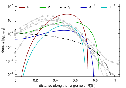
Figure 3: Density profiles of the basic building-block morphologies along the axis through the $\rho_{\rm max}$. Morphologies are constrained to have the same mass and average (RMS) expansion velocity. In gray: density profiles along the radial lines through the maximum density of the dynamical ejecta from neutron star mergers (Rosswog et al., 2014).

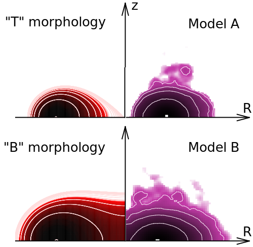
Figure 4: Morphologies “T” (toroidal) and “B” (biconcave; left panels) in comparison with toroidal axisymmetrized models from Rosswog et al. (2014) (right panel; also used in Wollaeger et al., 2018; Heinzel et al., 2021).

Table 1: Nondimensional shape factors $C_{v}$ and $C_{\rho}$ (see Eq. (3)).

Morphology	$C_{v}$	$C_{\rho}$
“H” – hourglass	1.028850	5.367093
“P” – peanut	1.079134	0.183475
“B” – biconcave	0.986012	0.0222324
“T” – torus	1	0.810569
“S” – sphere	1.914854	0.223138

Although the variety of possible morphologies is limitless, we have picked a few morphologies that are motivated by the astrophysical setting and easy to set up. Figure 2 depicts the five baseline axisymmetric morphologies: two prolate (H "hourglass," P "peanut"), one spherical (S), and two oblate (B "biconcave," T "torus"). The density for each model is given in velocity space axisymmetric coordinates ${\{v_{r},\theta\}}$ using the level function for a family of Cassini ovals:

$$\rho(v_{r},\theta)=\rho_{0}\left(\frac{t}{t_{0}}\right)^{-3}\times\begin{cases}(q-\bar{v}_{r}^{4}-2\bar{v}_{r}^{2}\cos{2\theta})^{3}\;\;\;{\rm prolate\,shapes},\\ (q-\bar{v}_{r}^{4}+2\bar{v}_{r}^{2}\cos{2\theta})^{3}\;\;\;{\rm oblate\,shapes},\end{cases}$$ (1)

The value $q=0$ gives a "figure-eight" shape, which if rotated around the $z$-axis produces our "H" and "T" morphology for the prolate and oblate cases, respectively. We use ${q=1}$ for the "P" and ${q=1.5}$ for the "B" morphologies (see Fig. 2). The spherical morphology "S" is specified by the “cubed inverted parabola” density profile, introduced in Wollaeger et al. (2018):

$$\rho(v_{r})=\rho_{0}\left(\frac{t}{t_{0}}\right)^{-3}\left(1-\bar{v}_{r}^{2}\right)^{3}\;\;\;\text{-- spherical shapes.}$$ (2)

In equations (1-2), $\rho_{0}$ sets the density scale, $\bar{v}_{r}=v_{r}/v_{0}$, and $v_{0}$ sets the velocity scale. These dimensional constants are connected with the ejecta mass $m_{\rm ej}$ and rms expansion velocity $v_{\rm ej}$ as follows:

$$v_{0} =C_{v}v_{\rm ej}, \rho_{0} =C_{\rho}\frac{m_{\rm ej}}{v_{\rm ej}^{3}t_{0}^{3}},$$ (3)

where the nondimensional shape factors $C_{v}$ and $C_{\rho}$ are listed in Table 1 for each of the morphologies.

Models with the same mass and average expansion velocity can possess very different density profiles. The latter are shown in Figure 3 for our five basic morphologies along their axes that pass through $\rho_{\rm max}$. The maximum densities vary by nearly two orders of magnitude between S and H morphologies, with the S(H) morphology having the lowest(highest) maximum density. For comparison with numerical simulations, Figure 3 also presents spherically averaged density profiles (in gray) of the dynamical ejecta from neutron star merger simulations of Rosswog et al. (2014) (also used in Wollaeger et al., 2018, see their Fig. 2). Differences in the density from simulations vary by an order of magnitude. Although variability in our models may be somewhat exaggerated, it is not unreasonable to expect it for other ejecta generation scenarios. Our choice of morphologies attempts to capture this diversity.

The spherical and prolate morphologies are motivated by simulations of post-merger outflows (e.g. Perego et al., 2014; Martin et al., 2015), which in general tend to concentrate toward the polar regions. Another case of prolate morphology is the “squeezed” collisional ejecta in the polar regions (Oechslin et al., 2007; Sekiguchi et al., 2016; Kasen et al., 2017). The oblate morphologies are motivated by simulations of tidally expelled dynamical ejecta, which are naturally concentrated toward the merger plane (Rosswog et al., 2014; Sekiguchi et al., 2016). Figure 4 compares the adopted toroidal morphologies “T” and “B” to the simulated models A and B from Rosswog et al. (2014) (also used in Wollaeger et al., 2018; Heinzel et al., 2021).

Our one-component models assume uniform composition and are constructed by rotating Cassini ovals around vertical axis as specified above. Although we expect multiple components in the true outflows, by simulating these one-component models, we can better understand the impact of geometry, such as the effects of the surface area or high-density regions. This allows for a better assessment of the impact of superimposing morphologies (e.g. lanthanide curtain). In addition, these nonspherical one-component models can be directly compared to other models in the literature (such as those studied in Perego et al., 2017; Darbha & Kasen, 2020; Zhu et al., 2020).

2.3.2 Two-component models

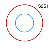
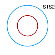
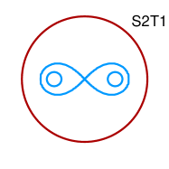
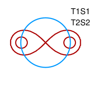
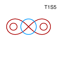
Figure 5: Schematics of the adopted two-component combinations of morphologies in the meridional plane. The first letter represents abbreviation of the neutron-rich (low-$Y_{e}$) outflow morphology, while the second letter stands for the higher-$Y_{e}$ outflow shape. The low-$Y_{e}$ (high-$Y_{e}$) component is represented by the red (blue) contour. The first (second) digit encodes mean expansion velocity of the low-$Y_{e}$ (high-$Y_{e}$) component: ${1=0.1\,c}$, ${2=0.2\,c}$, and “5” designates ${0.05\,c}$. This is reflected in the relative sizes of the components.

We next combine our one-component morphologies to have a suite of two-component (mixed) models, with overlapping high-$Y_{e}$ and low-$Y_{e}$ compositions. In the mixed models, we only pick three basic morphologies: S, P, and T (combinations with H instead of P and B instead of T produce very similar results). The selected combinations are outlined in Fig. 5, with the low-$Y_{e}$ and high-$Y_{e}$ compositions shown in red and blue, respectively. In the model names, the first and second letters stand for morphology of the low-$Y_{e}$ and high-$Y_{e}$ components, respectively, and the number designates the first significant digit in the mean velocity of expansion for the corresponding component. More exactly, "1" designates a mean expansion velocity of ${0.1\,c}$, "2" designates ${0.2\,c}$, and "5" designates ${0.05\,c}$. For example, T1S2 stands for a model with a toroidal low-$Y_{e}$ component with a mean expansion velocity ${0.1\,c}$ and a spherical high-$Y_{e}$ component with a mean expansion velocity ${0.2\,c}$. We consider a variety of masses for the blue and red components, with the baseline, default mass for either of the components being ${0.01\ M_{\odot}}$.

Each superposition of the components represents a specific scenario in outflow configurations. For instance, the TS (TP) morphologies can model a case when tidal dynamical ejecta has a toroidal shape, while the secondary wind outflow is spherical (axially focused). Indeed, recent ab initio simulations of remnant accretion disks produce axially elongated outflows with spatially variable neutron richness, such that high-$Y_{e}$ ejecta expands along the axis, while low-$Y_{e}$ ejecta tends toward the equatorial plane (Fernández & Metzger, 2013; Miller et al., 2019). The bi-spherical models S1S2 (S2S1) represent the simpler scenario of isotropic two-component outflow, in which high-$Y_{e}$ (low-$Y_{e}$) overtakes the other component, forming an outer envelope and obscuring it (Fernández & Metzger, 2016). Some studies (Wanajo et al., 2014) have suggested that the neutron fraction in a fast-moving interaction component, also known as “squeezed” dynamical ejecta (Goriely et al., 2011; Korobkin et al., 2012), can be reset to higher values by the intense heating and positron captures, which become available in abundance at high temperatures. Morphologies T1S2, S1S2 and P1S2 represent this scenario in our models. The models P1S2 and S2P1 represent polar outflow of one type, enveloped by a spherical outflow of the other type. The S2P1 scenario can be realized if initial low-$Y_{e}$ ejecta is fast and isotropic (Sekiguchi et al., 2016), and secondary high-$Y_{e}$ ejecta is slow and prolate. The slow component can be realized by neutrino-driven wind with prolate morphology, either from a transient hypermassive neutron star (Perego et al., 2014), or an accretion disk (Miller et al., 2019). Overall, these configurations represent a reasonably exhaustive set of outflow scenarios that can happen in neutron star mergers. However, they are still limited to axisymmetry. This may be too constraining for kilonovae from neutron star–black hole mergers, where even more diversity is expected due to the strong non-axisymmetric nature of the ejecta in some cases (Kyutoku et al., 2013; Perego et al., 2017; Zhu et al., 2020).

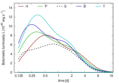
Figure 6: Integral bolometric luminosity (summed over all angular bins, as a function of time for the five single-component morphologies and the low-$Y_{e}$ (neutron-rich, solar r-process residuals) composition. Full network heating, density-dependent thermalization, and detailed suite of opacities is used.

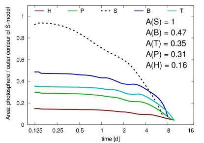
Figure 7: Area of the receding diffusion surface relative to the area of the outflow boundary of equivalent spherical model with the same mass and average expansion velocity, as a function of time, for the range of single-component models with low-$Y_{e}$ composition. The labels show the area of the outer surface of the morphologies relative to the spherical model.

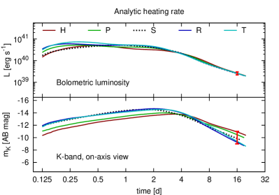
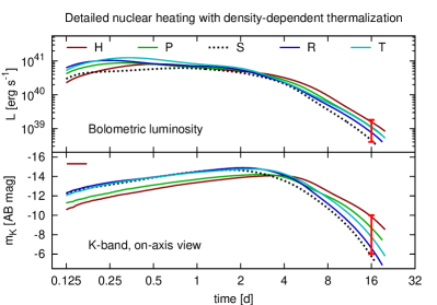
Figure 8: Angle-integrated bolometric luminosity (top panels) and $K$-band magnitudes for single-component morphologies of the same mass and velocity, computed with analytic heating prescription and uniform thermalization (left) vs detailed nuclear heating input with density-dependent thermalization (right). At late times, such as 16 days (highlighted in red), bolometric luminosity is not dependent on geometry when an analytic heating rate is used. For detailed nuclear heating with density-dependent thermalization (right panels), there is significant morphology-dependent variability in bolometric luminosity. Unlike bolometric light curves, the broadband ones, such as the $K$ band displayed here, show strong dependence on morphology in both cases (see the main text for discussion).

3 Results

Here we explore the range of possible kilonova signals based on the selected suite of ejecta morphologies and two representative compositions, separately expected to produce the “blue” and “red” kilonova. For the majority of simulations, we take the mass of either one or both components to be $0.01\,M_{\odot}$, in order to put more focus on the effects of ejecta geometry. Below, we first study single-component models and then proceed to two-component models.

3.1 Single-component Models

Figure 6 shows the evolution of angle-integrated bolometric luminosity for the one-component axisymmetric morphologies. The departure from spherical symmetry can have a large impact on the peak time and luminosity: B and T morphologies turn out to be brighter than the spherical model by a factor of two, and only need half of the time to reach their peak luminosity. The trend in brightness and peak epoch is set by the temperature of the outer radiative layer and, to a lesser degree, by the ejecta surface area. This can be inferred from Figure 7 which shows the ratio of the diffusion surface area to the area of the outer boundary of equivalent spherical model, as a function of time. It is clear that the surface area is not the dominant factor in deciding the peak brightness and epoch. The diffusion surface here is defined as enclosing the opaque “core” of the ejecta where photons are escaping slower than local expansion and are therefore trapped (Grossman et al., 2014). As the expansion progresses, the diffusion surface (along with the photosphere) recedes inwards until the entire bulk becomes exposed and transparent. To better understand the uncertainties in what sets the brightness of single-component models, we present a more extended discussion of these aspects in Appendix B.

Table 2: Ejecta masses inferred using equation 4, for single-component and mixed morphologies. The second column shows the mass (masses) of the single component (low-$Y_{e}$ component + high-$Y_{e}$ component) in percents of the Solar mass (${0.01\,M_{\odot}}$).

Model		top orientation			side orientation			average
morphology	$m_{l}+m_{h}$	$L_{\rm peak}$	$t_{\rm peak}$	mass	$L_{\rm peak}$	$t_{\rm peak}$	mass	$L_{\rm peak}$	$t_{\rm peak}$	mass
	$[0.01M_{\odot}]$	[$10^{40}$ erg/s]	[d]	$[0.01M_{\odot}]$	[$10^{40}$ erg/s]	[d]	$[0.01M_{\odot}]$	[$10^{40}$ erg/s]	[d]	$[0.01M_{\odot}]$
low-$Y_{e}$ composition: H1	1	5.4	1.12	2.6	6.5	1.09	3.2	6.4	1.11	3.2
P1	1	5.7	0.72	1.4	8.1	0.70	2.1	7.4	0.70	1.9
B1	1	12.1	0.59	2.5	7.0	0.54	1.2	9.0	0.56	1.7
T1	1	14.7	0.75	4.7	7.0	0.69	1.7	10.4	0.73	3.0
H2	1	9.1	0.50	1.4	7.1	0.52	1.1	8.1	0.52	1.3
P2	1	9.2	0.31	0.7	8.3	0.32	0.6	8.7	0.32	0.7
B2	1	11.5	0.26	0.7	9.5	0.24	0.5	10.3	0.24	0.6
T2	1	14.8	0.37	1.6	10.2	0.31	0.8	12.4	0.34	1.1
S2	1	6.1	0.78	1.7	6.1	0.78	1.7	6.1	0.78	1.7
high-$Y_{e}$ composition: H1	1	24.3	0.79	9.3	29.7	0.83	12.5	29.2	0.82	12.0
P1	1	27.1	0.56	6.3	41.8	0.57	10.6	38.0	0.57	9.6
B1	1	68.9	0.47	14.5	34.1	0.43	5.4	47.7	0.46	8.9
T1	1	68.9	0.54	17.9	30.7	0.50	6.0	48.3	0.53	11.3
H2	1	47.7	0.40	7.3	40.2	0.47	7.6	44.2	0.44	7.7
P2	1	52.1	0.28	4.6	53.6	0.32	5.9	54.5	0.31	5.7
B2	1	80.4	0.26	7.0	54.8	0.21	3.3	65.3	0.23	4.7
T2	1	83.4	0.30	9.0	51.6	0.25	4.0	67.2	0.28	6.2
S2	1	41.9	0.37	5.5	41.9	0.37	5.5	41.9	0.37	5.5
low-$Y_{e}$ + high-$Y_{e}$: P1S2	$1+1$	106.3	0.24	8.9	105.7	0.24	8.8	105.9	0.24	8.8
S2P1	$1+1$	5.1	4.06	17.7	4.2	5.07	19.8	4.5	4.69	18.9
S1S2	$1+1$	103.4	0.23	7.6	103.4	0.23	7.6	103.4	0.23	7.6
S2S1	$1+1$	4.6	4.12	16.3	4.6	4.12	16.3	4.6	4.12	16.3
S2T1	$1+1$	4.3	4.91	19.8	4.8	4.37	18.4	4.6	4.53	18.8
T1P1	$1+1$	49.2	0.65	15.8	43.7	0.67	14.3	44.9	0.66	14.4
T2P1	$1+1$	67.1	0.64	22.0	14.7	0.60	3.3	41.1	0.62	12.0
T2P2	$1+1$	103.1	0.31	12.6	65.8	0.37	9.4	78.3	0.35	10.5
T2P1	$1+1$	90.1	0.81	45.1	19.4	0.80	7.1	54.8	0.80	24.6
T1S1	$1+1$	66.5	0.39	10.3	55.6	0.29	5.4	58.8	0.32	6.8
T1S2	$1+1$	107.2	0.25	9.0	105.3	0.24	8.7	106.1	0.24	8.8
T2S1	$1+1$	76.7	0.47	16.1	12.6	0.30	0.9	37.6	0.43	6.1
T2S2	$1+1$	110.4	0.25	9.8	82.3	0.21	5.2	92.8	0.23	6.8
T2P5	$1+1$	64.2	1.07	46.7	3.8	0.33	0.27	32.9	1.11	22.1
T2S5	$1+1$	45.8	1.26	39.8	3.8	0.32	0.25	19.9	1.34	16.3
T2P2	$1+2$	135.6	0.38	23.4	93.4	0.44	18.4	108.5	0.41	20.2
T2S1	$1+2$	104.8	0.57	32.1	17.1	0.35	1.7	51.1	0.51	11.6
T2S2	$1+2$	164.7	0.29	19.1	131.3	0.23	10.7	143.6	0.26	13.7
T2P1	$1+3$	106.9	0.93	68.5	23.1	0.94	11.2	65.0	0.93	37.7
T2P2	$1+3$	161.3	0.44	35.6	111.2	0.50	28.3	129.3	0.46	29.9
T2S1	$1+3$	125.2	0.65	48.1	20.4	0.36	2.2	61.1	0.58	17.4
T2S2	$1+3$	204.9	0.31	28.3	168.8	0.25	16.4	182.1	0.28	20.3
T2P5	$1+0.5$	48.2	0.85	23.0	3.8	0.32	0.2	24.6	0.87	10.8
T2P1	$1+0.5$	50.8	0.51	11.4	11.6	0.47	1.7	31.5	0.50	6.2
T2S5	$1+0.5$	35.0	0.99	19.9	3.8	0.33	0.26	15.4	1.05	8.3
T2S1	$1+0.5$	45.9	0.63	13.7	3.8	0.31	0.25	19.7	0.61	4.8

Our single-component simulations assume the same mass, $0.01\,M_{\odot}$, and yet produce a wide range of peak times and luminosities, as shown in Table 2. Several groups have developed formulae that relate the peak luminosity and time of peak luminosity to the mass, expansion velocity, and opacity of the ejecta (Grossman et al., 2014; Wollaeger et al., 2018). To understand how the variation in the light curve leads to errors in the mass estimates, we have inverted the pair of formulae, Eqs. (27)–(28) from Wollaeger et al. (2018), deriving the mass inferred from the light curves produced in the models:

$$m_{2}=\left(\frac{t_{\rm peak}}{1\,d}\right)^{1.5}\left(\frac{L_{\rm peak}}{2.8\times 10^{40}\,{\rm erg}\,{\rm s}^{-1}}\right)^{1.2}\left(\frac{\kappa}{10\,{\rm cm}^{2}\,{\rm g}^{-1}}\right)^{0.2}.$$ (4)

where $t_{\rm peak}$ and $L_{\rm peak}$ are the time and bolometric luminosity, respectively, at the peak, $\kappa$ is the average opacity, and the resulting mass is in units of $0.01\,M_{\odot}$.

We can now quantify the uncertainty of the ejecta mass that can be inferred from the peak times and luminosities using Eq.(4). Kilonova observations rising above the afterflow of gamma-ray bursts (GRBs) at late times will consist of only a few observations, and comparisons to integrated solutions such as equation (4) are the only option for inferring ejecta mass. If more observations become available, more accurate methods, such as spectral fitting or light-curve matching, are definitely more appropriate. However, it is far more likely that the majority of kilonovae will be caught either when they are near their peak brightness, or at late times in follow-up observations. Specifically, for off-axis events, it is more likely that the kilonova will be observed near peak brightness, while for GRB follow-ups, it is likely to be observed at late times after the GRB afterglow dims. As we demonstrate below, the late-time light curves are at least as sensitive to morphologies as the peak-time light curves.

Inserting the peak parameters of our model light curves, we see that a mass that could be inferred from an observation using this formula can range over several orders of magnitude (see Table 2). The inferred mass only weakly depends on the effective opacity: for the calculations in Table 2, we assumed $\kappa=10{\rm\,cm^{2}g^{-1}}$.

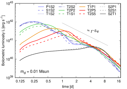
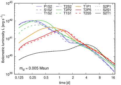
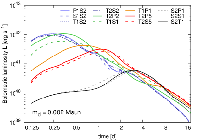
Figure 9: Angle-integrated bolometric luminosity as a function of time for twelve mixed morphologies, and three different masses of the low-$Y_{e}$ (neutron-rich) component. The top plot shows $\propto\,t^{-5/4}$ trend.

Since the bolometric light curves in Fig. 6 are, in the absolute sense, converging at late times, it may seem that a better strategy to constrain the masses would be to use the late-time light curves. However, it turns out that relative luminosities and broadband magnitudes at late times are similarly sensitive, if not more sensitive, to morphologies than the peak times. Figure 8 shows the bolometric light curves on a logarithmic scale, as well as the light curves in the infrared $K$-band, for two models of heating: analytic heating prescription (left panels) and full network heating with density-dependent thermalization (right panels). Because morphologies have different densities, the density-dependent thermalization in the latter introduces variability in the late-time light curves by about half an order of magnitude for the different models considered here (see also Kasen & Barnes, 2019; Barnes et al., 2020, on the importance of thermalization at late times).

Furthermore, even if the bolometric light curves converge for different morphologies, the broadband light curves do not have to. Fig. 8, left panel, shows the bolometric and $K$-band light curves for the case when an analytic power-law heating is prescribed, which does not depend on density. The broadband light curves still show a substantial degree of variability: by about 2 mag in $K$-band at 16 days. This is because the same luminosity can be produced at different temperatures, and the latter depends on the cooling history of the ejecta. Because optically thin ejecta are cooled inefficiently, their temperature maintains strong dependence on the previous state, and by extension, on the morphology. This temperature variability for the same bolometric luminosity is an additional factor of uncertainty in the determination of the masses. Notice that in this work, we make the assumption of LTE, both in the calculation of opacities and in the local emissivity. This assumption is likely to be violated at late times, making the notion of a single temperature meaningless, and adding to the uncertainty in masses. If the late-time conditions that determine the atomic level populations are optically thin, then the charge state distribution will likely shift toward more neutral species compared to the LTE case, due to a reduction in the effective ionization resulting from radiative processes. This difference typically leads to absorption line features that occur at lower photon energies for non-LTE conditions, with a corresponding shift in the emission features. It is difficult to make more specific, quantitative predictions about non-LTE effects on the photometry without doing actual simulations, which we reserve for future work. Another uncertainty comes from the problem of reconstructing bolometric light curves from photometry, which will be scarce at late times and highly dependent on transient broadband spectral features and large deviations from the blackbody. If one adds uncertainties in the unknown nuclear heating, which may reach an order of magnitude (Zhu et al., 2019; Barnes et al., 2020), in combination with the morphology-specific variability, mass inference from late-time bolometric luminosity becomes quite problematic. Nevertheless, these complexities should not deter observers from obtaining the late-time data. On the contrary, accurate deep photometry and spectra at late times are crucial to improve our understanding of the masses and morphologies of the ejecta.

We conclude that without strong observational constraints on the geometry of the ejecta, one can artificially infer larger masses from nonspherical explosions, which have higher densities and correspondingly higher temperatures, or higher apparent surface areas (see discussion in Appendix B). If we cannot constrain the composition, the uncertainty can be even larger.

3.2 Two-component Models

Combining two components with different morphologies enables a much wider class of kilonovae. The range of mass estimates that can be inferred from limited information such as peak brightness and epoch now spans almost three orders of magnitude (see Table 2). The range of inferred masses can vary strongly even within the same model. For example, in the model T2P5 with fast toroidal lanthanide-rich component and slow high-$Y_{e}$ outflow, the mass estimate ranges between 0.002 and 0.23 $M_{\odot}$, depending on orientation. In the side view, the toroidal component with lanthanide-rich composition has a very high opacity that completely obscures the bluer and brighter secondary outflow, which in turn leads to a smaller inferred mass. This is the lanthanide “curtaining”: high-opacity lanthanide-rich ejecta in front of more luminous outflow act as a “curtain,” hiding the blue kilonova for a range of viewing angles (Kasen et al., 2015). At the same time, the top view leads to overestimated mass because of the brighter transient, since the secondary outflow is revealed and the toroidal component has a large projected area.

In Fig. 9, we plot the angle-integrated bolometric luminosity versus time for all mixed models. It shows that the impact of morphology can be a dominant indicator of the brightness, even when summed over viewing angle. In every model where the low-$Y_{e}$ ejecta is more extended than the high-$Y_{e}$ ejecta (S2S1, S2P1 and S2T1), the high lanthanide opacities block all of the optical emission, causing the peak luminosity to be an order of magnitude dimmer than the rest of the models. On the other hand, models in which the high-$Y_{e}$ wind component is spherical and more extended (S1S2, P1S2 and T1S2) are the brightest, but also peak too soon.

The rest of the models lie in between these two extremes. The panels in Figure 9 correspond to three different masses of the lanthanide-rich component: 0.01, 0.005, and 0.002 $M_{\odot}$, while the mass of the high-$Y_{e}$ component is kept fixed at ${0.01\,M_{\odot}}$. In every panel, the models that lie between the two extremes span a wide range of peak times (from 0.2 to 6 days) and two orders in luminosity. For all models, there is a trend of an approximate inverse correlation between peak time and luminosity:

$$L_{\rm peak}\propto t_{\rm peak}^{-5/4},$$ (5)

which also follows from Eq. (4) for fixed mass and opacity. This result shows that the effect of mixing morphologies is degenerate with the expansion velocity or effective opacity.

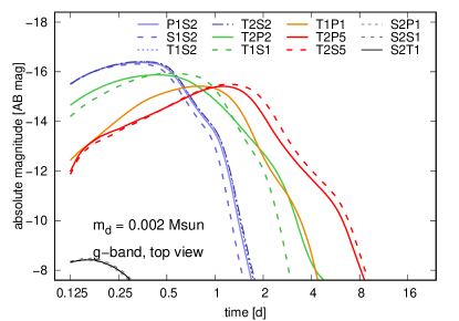
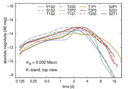
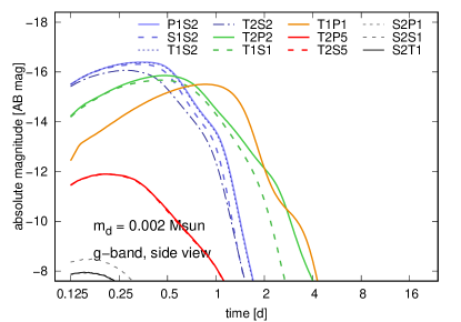
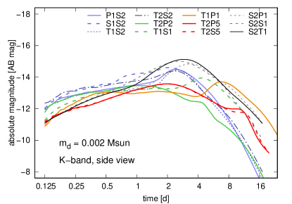
Figure 10: Broadband light curves ($g$ and $K$ bands) for the 12 mixed morphologies with the lanthanide-rich (low-$Y_{e}$) component mass $0.002\,M_{\odot}$. The top row shows the on-axis, or "top" orientation, and the bottom panels show the "side" orientation toward the observer.

Notice that for the cases considered, the relative mass of the lanthanide-rich component has very little effect on the light curves. The only exception is the position of the luminosity peak for models S2P1, S2S1 and S2T1, in which this component is spherical and more extended, hiding the high-$Y_{e}$ outflow. This again illustrates that in many cases, the mass of the ejecta is subdominant in determining the light curves compared to the morphology. The only cases where the effect of the lanthanide-rich component is most pronounced are when it completely blocks the blue component. If the lanthanide-rich component is the interior one, or if it fails to block emission from the other component, its effect on light curves is minimal. A lower mass of the lanthanide-rich component in these models leads to a brighter and earlier peak, due to the fact that with lower mass it becomes transparent sooner, exposing the brighter high-$Y_{e}$ outflow. This effect is again degenerate with changing the expansion velocity or opacity, which further complicates ejecta mass estimates.

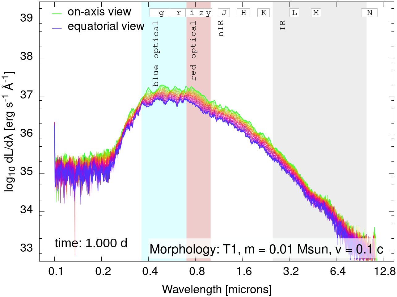
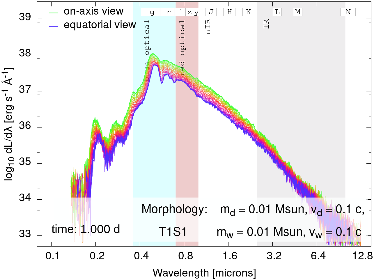
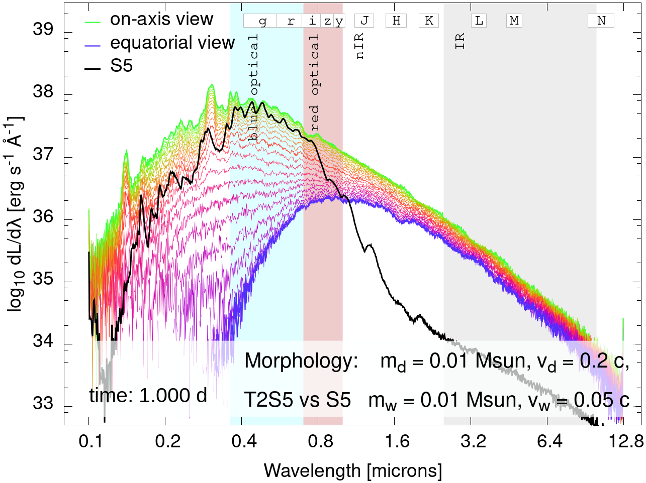
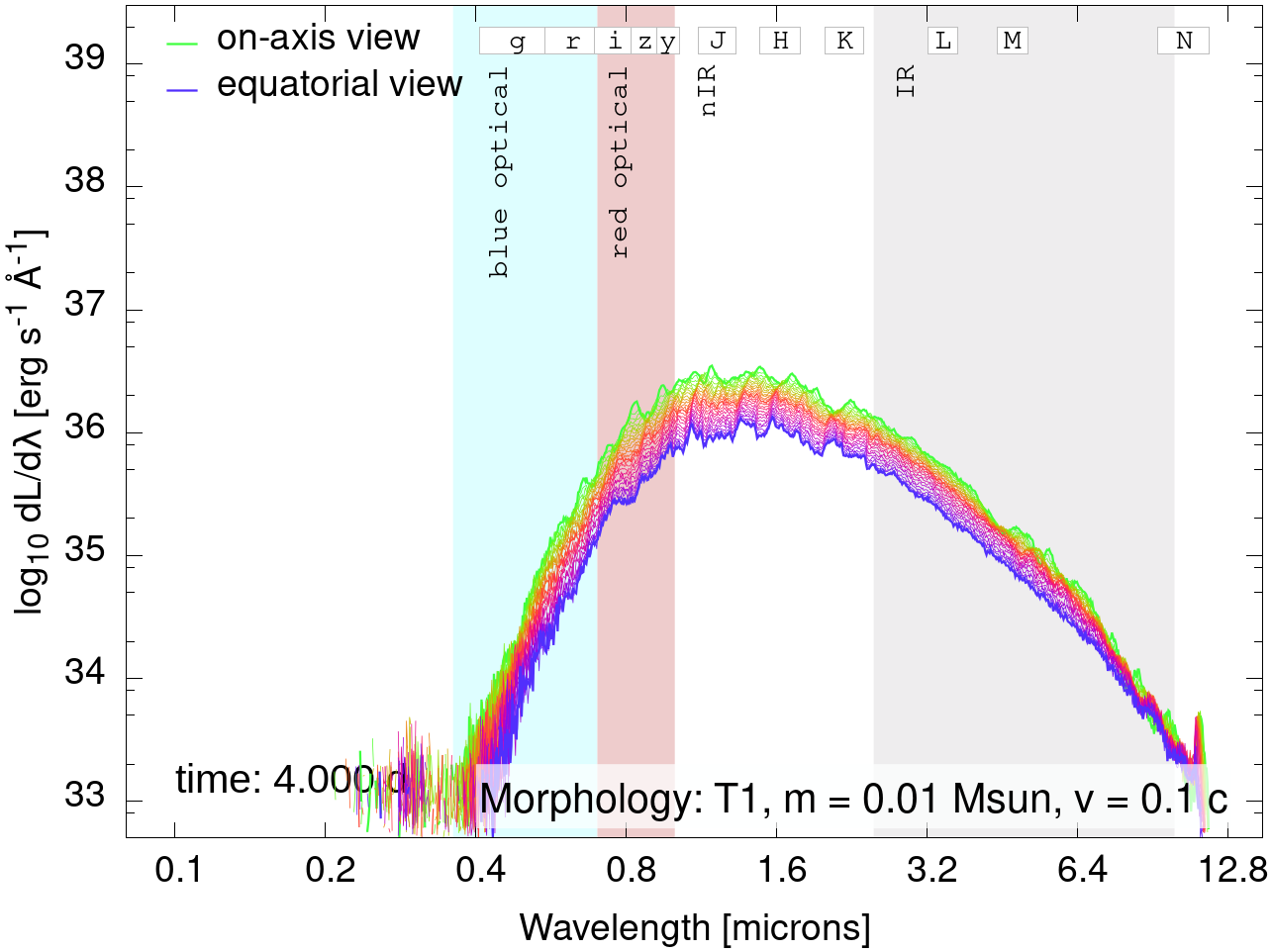
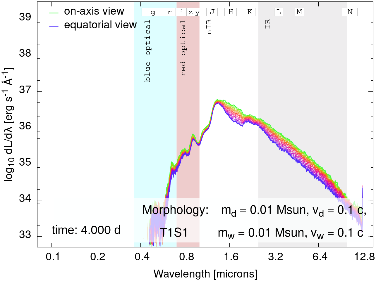
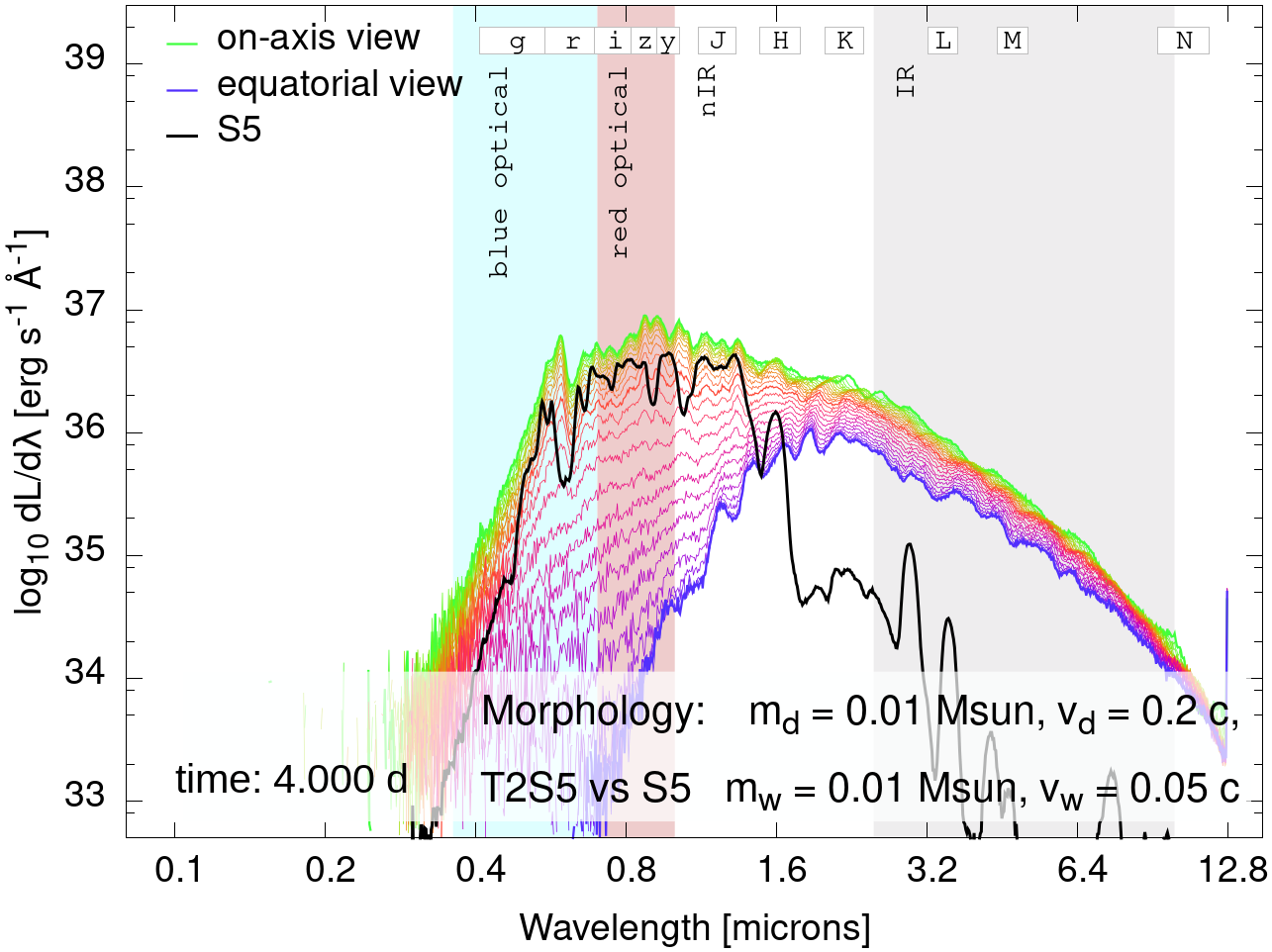
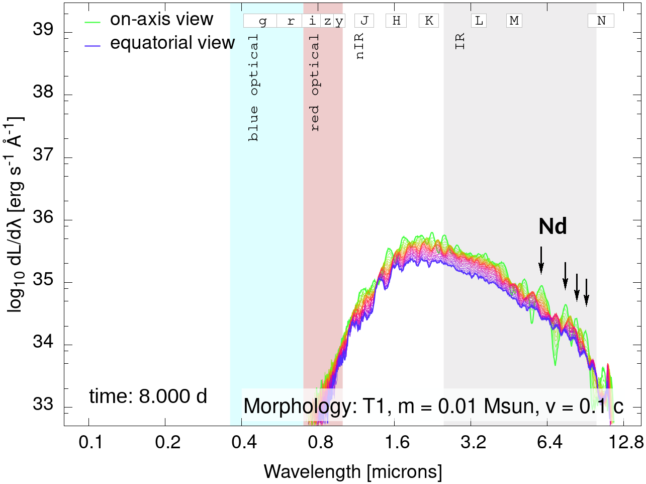
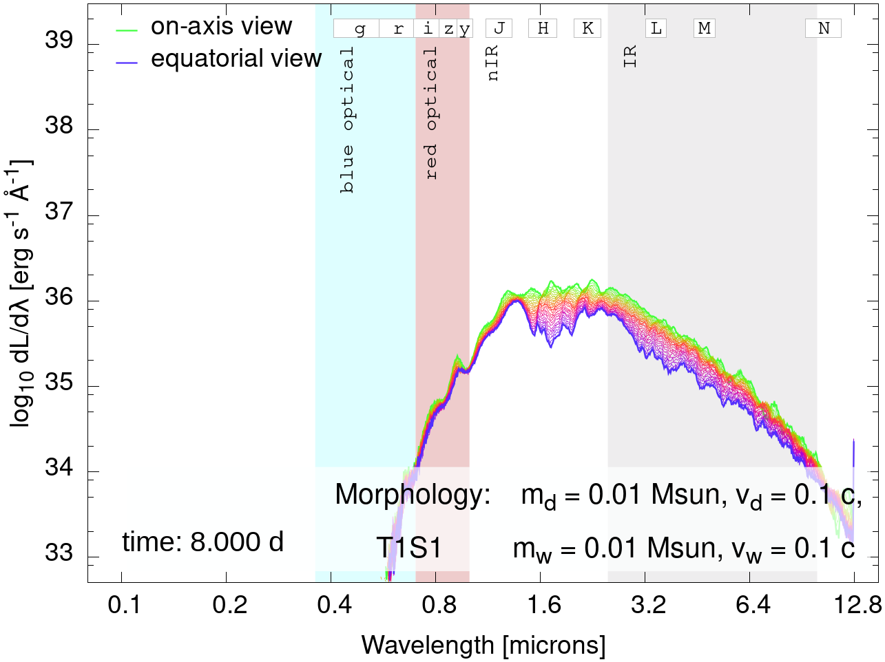
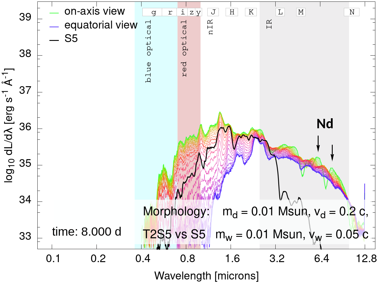
Figure 11: Kilonova spectra at 1, 4, and 8 days for a single-component model "T" (left) and two-component "TS" morphologies (middle and right), for the full range of viewing angles. The middle and right components differ by the expansion velocities: in the middle column, both components have the same expansion velocity ${v_{d}=v_{w}=0.1\,c}$. In the right column, the velocity of the high-$Y_{e}$ "wind" ${v_{w}=0.05\,c}$ is much less than that for the low-$Y_{e}$ outflow ${v_{d}=0.2\,c}$. The differences in the velocities for the two outflows in the right column cause strong variation on the spectrum due to lanthanide curtaining or the high-$Y_{e}$ outflows by the more extended lanthanide-rich toroidal component. This is the case that manifests the strongest angular dependence, while for the rest of the models, the angular dependence is very moderate. In the right column, the black solid line shows just the spherical high-$Y_{e}$ component "S5," without the toroidal part. It illustrates the light focusing by the toroidal component, which causes the blue emission to preferentially diffuse toward the axis. The black vertical arrows in the bottom row point to the P Cygni features in mid-IR generated by peaks of the wavelength-dependent opacity of Nd.

It is unlikely that measuring the light curves in a broad range of bands will be sufficient to lift these degeneracies. Fig. 10 shows the optical $g$- and nIR $K$-band light curves for all mixed morphologies and a low-$Y_{e}$ component mass of ${0.002\,M_{\odot}}$. In the $g$-band, it is easy to distinguish models with more extended spherical lanthanide-rich ejecta (S2P1, S2S1 and S2T1, black lines): they are very strongly suppressed in this band for all orientations. These models instead produce the brightest red kilonova in the $K$ band. The rest of the models peak between 0.5 and 2 days in the $g$ band with magnitudes $-15$ to $-16$ mag, and rapidly decay by about 4 days. Models T2P5 and T2S5 present a notable exception: they radiate longest in the $g$ band for the "top" orientation and are strongly suppressed for the "side" view. This strong angular dependence is due to lanthanide curtaining.

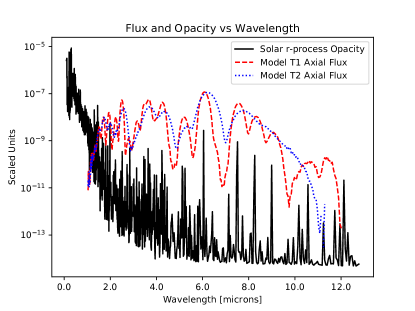
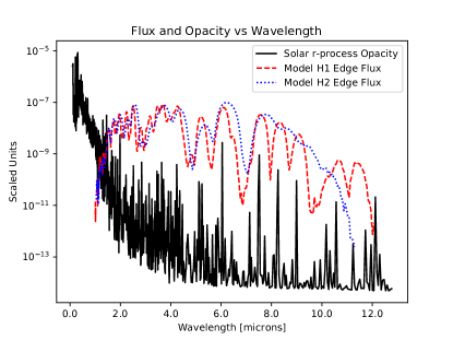
Figure 12: Axial-view flux for model T and edge-view flux for model H, along with scaled opacity, versus wavelength. These models are moving at an average speed of $0.1c$ or $0.2c$. Relative to the $0.1c$ simulations, line emission blending is enhanced in the $0.2c$ simulations. Line features in the spectra are more visible in the axial (edge) view for model T (H), where the velocity toward the observer is slower. A majority of the tall lines above $\sim 4\,\mu$m are from Nd, which is setting the IR emission at late time in our models (cf. Fig. 8 in Even et al., 2020).

Most of our mixed models do not show pronounced dependence on the viewing angle beyond that of single-component models, where variability of about 1 mag can be attributed to the projected area of the photosphere (Grossman et al., 2014; Darbha & Kasen, 2020). This is because lanthanide curtaining is only partial: T1S1 is a typical representative of this scenario. In Figure 11, we compare its spectra with that of a single-component model T which lacks the high-$Y_{e}$ contribution. At early times, the spectra for model T1S1 are significantly brighter and bluer than for the model T. The impact of the high-$Y_{e}$ outflow also extends to late times, maintaining bluer emission relative to T. The latter behavior and the much weaker angular dependence of the blue wing of T1S1 at late time are the result of optical reprocessing by the lanthanide-free component. At $\gtrsim$8 days, the viewing angle-dependent P Cygni features of Nd lines start to form in the mid-IR. However, these features only appear for the "top" orientation, as in this case the differential expansion velocity toward the observer is only about ${0.1\,c}$ (more about this at the end of this Section).

In some mixed-morphology scenarios, the viewing angle dramatically affects the spectrum and observed kilonova magnitudes. This is illustrated with the model T2S5 (Fig. 11, right column). Here the lanthanide-rich component is much more extended, curtaining the high-$Y_{e}$ outflow for some orientations. This behavior is unlike that observed for T1S1, where both components are always visible. Moreover, the blue wing of T2S5 for the top orientations is much brighter than that of just the spherical low-opacity component S5 (its spectrum is shown with a solid black line in Fig. 11). This appears to be because the lanthanide-rich toroidal component additionally redirects the flux toward low-opacity polar regions (also observed in the kilonova models of Kawaguchi et al., 2018). No reddening of the redirected flux is observed, because the photons effectively return to the low-opacity region and get reemitted in blue wing before escaping down the gradient of the optical depth. At $\gtrsim$8 days, pronounced P Cygni features of Nd lines start to develop at the mid-IR wing of the spectrum, resembling those of model T, but are twice as broad due to a higher line-of-sight expansion velocity. This is in contrast with model T1S1 where these features are diluted by reprocessing in the enclosing high-$Y_{e}$ spherical component (bottom middle panel in Fig. 11).

The strong dependence on orientation for some mixed models directly projects onto broadband light curves. As can be seen in Figure 10, models T2P5 and T2S5 (shown in red), are strongly suppressed in the optical bands for the "side" orientation. On the other hand, for the "top" orientation, they show the same magnitude in the optical bands as the rest of the models. Moreover, they produce the longest-lasting blue kilonovae—due to the flux redirection mentioned above.

Because of the very high opacity of the lanthanides, a strong angular dependence persists even if the mass of the lanthanide-rich component is very small. In our models, it goes down to ${0.002\,M_{\odot}}$. This is shown in Figure 10, where the difference for the $g$ band is 4 mag between the top and side orientations. In nIR bands, such as the $K$ band shown in the right column of Figure 10, the difference is only 1 mag.

At late times, we observe P Cygni features (Castor & Lamers, 1979; Robinson, 2007) forming in the mid-IR wing of the spectra of one-component models and in the spectra of models where high-$Y_{e}$ and low-$Y_{e}$ components are well separated (T2P5 and T2S5). These features form around strong lines in the opacity and can be used to characterize both composition and morphology of the ejecta. Figure 12 overplots the opacity ${\kappa_{\lambda}}$ and the late-time spectra for single-component models T and H, each with velocities of ${0.1\,c}$ (denoted H1, T1) or ${0.2\,c}$ (denoted H2, T2). For the toroidal morphology T, the spectrum is shown from a top view and for the hourglass H from the side. The opacity is evaluated at $\rho=10^{-16}\,{\textrm{g}\ \textrm{cm}^{-3}}$, $T=1000$ K, and scaled by a constant factor to facilitate comparison with the spectra. The low-velocity models H1 and T1 produce narrow features due to less Doppler broadening or blending between emission peaks. The high-velocity models H2 and T2 appear to have a much less structured spectrum, in particular around $10\,\mu$m. These features clearly reflect spikes in the opacity profile, which in turn are produced by Nd at this density and temperature (cf. Fig. 8 in Even et al., 2020).

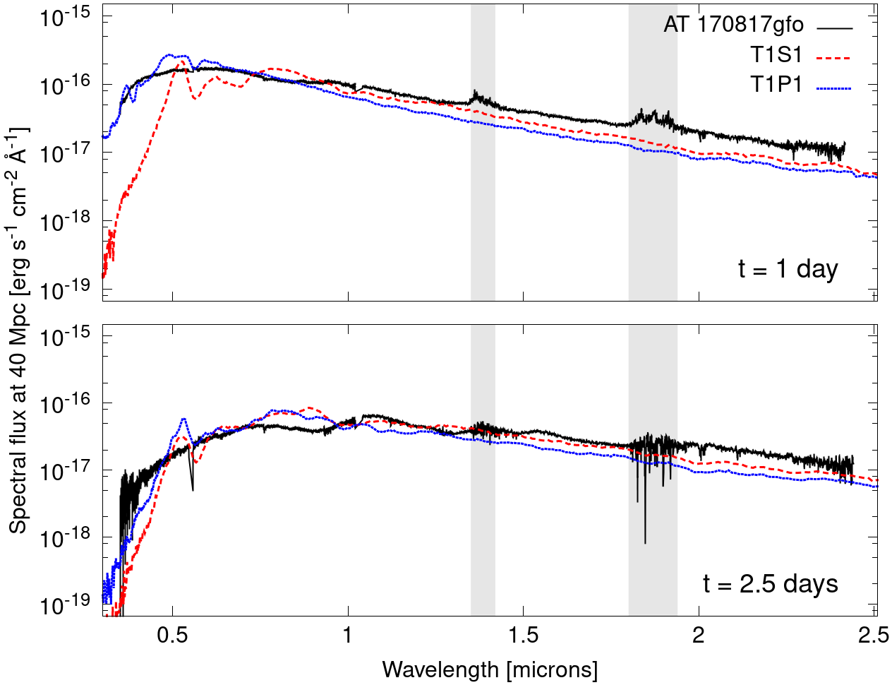
Figure 13: Model spectra for the two best-matching geometries at the epochs $t=1$ day and $2.5$ days in comparison with the spectrum measured for the kilonova AT 2017gtfo accompanying GW170817 (instrument: VLT/X-shooter; Pian et al., 2017). Both models have equal masses of the neutron-rich and neutron-poor components, $m_{d}=m_{w}=0.01\ M_{\odot}$ and are shown with on-axis view. Wavelength ranges with poor data quality for the observed spectra are marked in gray (see Pian et al., 2017, for details).

4 Conclusions

We study a set of analytically prescribed axisymmetric and spherically symmetric morphologies representative of neutron star merger ejecta using the multidimensional, multigroup Monte Carlo code SuperNu (Wollaeger & van Rossum, 2014) and detailed opacities from the LANL suite of atomic physics codes (Fontes et al., 2015, 2020). Our five representative basic shapes are obtained from the family of Cassini ovals in axisymmetry (see Fig. 2), rescaled to a given total mass and average expansion velocity. We model the merger ejecta with single- or two-component morphologies with two spatially uniform representative compositions producing “red” and “blue” contributions of the kilonova. Specifically, we focus on two compositions: a low-electron-fraction ($Y_{e}$) lanthanide-rich solar r-process residuals (Even et al., 2020), and a high-$Y_{e}$ composition with ${Y_{e}=0.27}$ (“wind 2” in Wollaeger et al., 2018). Compositions determine not only specific nuclear heating but also opacities of the material. The former is computed with the WinNET nuclear network (Winteler et al., 2012) with energy partitioning between radiation species and spatially dependent thermalization (Barnes et al., 2016; Rosswog et al., 2017; Wollaeger et al., 2018). For the latter, we employ a new suite of atomic opacities, which includes a complete set of lanthanides and uranium (Fontes et al., 2020).

The results of our study can be summarized as follows:

1. When detailed, temperature-dependent opacities are used, the morphology affects the light curve more than the mass and velocity of the ejecta. For the same mass and expansion velocity, switching between the different morphologies considered here leads to stronger variation in the peak time and luminosity than if we fixed the morphology and varied mass (by a factor of ten) or velocity (within $0.05-0.3\,c$ – see Fig. 6 and 9).

2. Because of this result, the ejecta mass cannot be correctly inferred solely from the peak bolometric luminosity and time. Our simulations show that the mass inferred from an effective gray-opacity formula can vary by an order of magnitude within one-component morphologies, and by three orders of magnitude for mixed models. Without strong constraints on the geometry of the ejecta, artificially large or small masses can be inferred from nonspherical explosions (see Table 2).

3. Morphological variability affects the peak luminosity in a way similar to varying the ejecta velocity or effective opacity. For a family of morphologies with the same mass and expansion velocity, the peak luminosity is inversely correlated with peak times: ${L_{\rm peak}\propto t_{\rm peak}^{-5/4}}$ (Fig. 5). The effect of mixing morphologies is degenerate with the effect of changing the average expansion velocity or effective gray opacity.

4. Unlike the gray-opacity case, in the models with detailed opacity, the temperature at the surface is more important in defining the peak properties than the projected area (see Appendix B for detailed analysis).

5. Density-dependent thermalization of radioactive heating adds an extra boost to the bolometric luminosity, increasing it by almost a factor of two. Therefore, a proper treatment of thermalization is as important as accurate composition-dependent nuclear heating rates (see also Barnes et al., 2016; Rosswog et al., 2017; Hotokezaka & Nakar, 2019).

6. It is difficult to achieve the lanthanide curtaining effect if the two components have similar expansion velocities (Kasen et al., 2015). In this case, only partial lanthanide curtaining is observed. The majority of our models are quite isotropic, except when the high-$Y_{e}$ component is much slower than the lanthanide-rich component (models T2S5 and T2P5 – see Fig. 11). Lanthanide curtaining is observed only in these models at low-latitude angles.

7. For the models with lanthanide curtaining, even a very small mass of $0.002\,M_{\odot}$ of lanthanide-rich material is sufficient to obscure the blue kilonova, because of the exceptionally high opacity of lanthanides (Kasen et al., 2013; Tanaka & Hotokezaka, 2013; Fontes et al., 2015). This is also consistent with the recent study of Nativi et al. (2020).

8. At late epochs ($\gtrsim$8 days), the models in which lanthanide-rich ejecta is more extended exhibit pronounced P Cygni features, allowing for the characterization of the composition and line-of-sight velocity of the ejecta (Fig. 12). Our results here confirm the findings of Kawaguchi et al. (2018). These P Cygni features are unambiguously unidentified with peaks in opacity of Nd, which has been shown to dominate the opacity of lanthanide-rich material (Fontes et al., 2020; Even et al., 2020).

9. Light reprocessing: in the case when the lanthanide-rich component is engulfed in a spherical high-$Y_{e}$ envelope, the blue kilonova becomes almost isotropic and the P Cygni features from Nd disappear (Fig. 11, middle column).

10. Light focusing by toroidal component: in the models with a more extended toroidal lanthanide-rich component, the light from the blue component is effectively funneled toward the axis such that the blue kilonova appears brighter (Fig. 11, right column).

Morphological freedom creates sufficient variability to crudely fit the early spectrum of kilonova GW170817 with the limited set of models that we presented in this study. In Figure 13 we demonstrate a “fit” to GW170817 spectra at $t=1-2.5$ days. The “best-matching” models appear to be T1S1 and T1P1. Clearly, tuning the velocities and masses of individual components, as well as the viewing angle, can significantly improve this result, which is beyond the scope of this paper (but see Heinzel et al., 2021). Fitting the late-time spectra is a continuing goal. This concept, yet again, demonstrates that a meaningful interpretation of kilonova light curves must properly account for morphological features, which should be informed by numerical simulations and observations.

We summarize the bolometric and broad band magnitudes at 1, 4, and 8 days for all models used in this study in Table 3 below. The complete suite of our models is available from the LANL CTA website.

Appendix A Model tables: magnitudes at days 1, 4, and 8

Table 3 lists the $r$- and $J$-band magnitudes and bolometric luminosity at days 1, 4, and 8 for top / side views.

Table 3: Top / side viewing bin for absolute AB magnitudes in the $r$ and $J$ bands and angle-integrated bolometric luminosity ($L_{\rm bol}$ [$10^{40}$ erg s^-1]) for our models.

$m_{l}+m_{h}$ Day 1 Day 4 Day 8 Model $[0.01\,M_{\odot}]$ $r$ $J$ $L_{\rm bol}$ $r$ $J$ $L_{\rm bol}$ $r$ $J$ $L_{\rm bol}$ low-$Y_{e}$ composition: H1 1 -13.2 / -13.3 -13.2 / -13.5 5.4 / 6.5 -10.6 / -10.3 -13.2 / -13.4 2.7 / 3.4 -4.3 / -4.5 -11.1 / -11.5 1.3 / 1.7 H2 1 -13.6 / -13.0 -13.9 / -13.8 7.2 / 6.2 -8.0 / -6.9 -13.0 / -12.7 3.0 / 3.1 -0.0 / 0.2 -10.0 / -8.6 0.8 / 1.0 P1 1 -13.2 / -13.4 -13.4 / -13.8 5.4 / 7.5 -9.1 / -9.0 -13.0 / -13.4 2.4 / 3.8 -0.7 / -0.6 -9.8 / -10.0 0.8 / 1.4 P2 1 -13.0 / -12.3 -14.1 / -14.1 6.2 / 6.3 -4.9 / -3.8 -12.1 / -11.5 2.2 / 2.8 0.1 / 0.1 -9.4 / -7.8 0.6 / 0.7 B1 1 -13.7 / -13.1 -14.2 / -13.6 9.7 / 5.4 -8.8 / -6.8 -13.5 / -12.3 5.2 / 2.1 0.2 / 0.4 -9.5 / -8.8 1.3 / 0.7 B2 1 -12.2 / -12.3 -14.4 / -14.1 8.7 / 6.0 -2.7 / -2.6 -11.1 / -11.1 3.0 / 1.7 0.0 / 0.0 -7.7 / -8.6 0.5 / 0.5 T1 1 -14.1 / -13.4 -14.4 / -13.6 13.8 / 6.3 -9.7 / -8.1 -13.8 / -12.6 5.4 / 2.1 0.1 / 0.3 -9.9 / -9.0 1.2 / 0.6 T2 1 -13.0 / -12.9 -14.6 / -14.1 10.4 / 6.1 -3.9 / -3.3 -11.7 / -11.3 3.0 / 1.6 -0.0 / 0.0 -8.2 / -9.0 0.6 / 0.5 high-$Y_{e}$ composition: H1 1 -14.3 / -14.7 -13.0 / -13.4 22.2 / 28.2 -12.9 / -13.1 -13.2 / -13.3 3.1 / 3.5 -9.2 / -9.1 -12.3 / -12.9 0.9 / 1.0 H2 1 -14.4 / -14.9 -13.7 / -13.7 16.9 / 17.7 -11.8 / -11.1 -12.8 / -13.2 2.0 / 1.9 -8.8 / -6.8 -11.9 / -12.6 0.7 / 0.7 P1 1 -14.3 / -15.0 -13.1 / -13.6 15.4 / 25.9 -12.1 / -12.6 -13.0 / -13.4 2.2 / 2.8 -8.2 / -7.7 -12.2 / -12.8 0.7 / 0.9 P2 1 -14.4 / -14.9 -14.1 / -14.4 13.6 / 14.7 -10.3 / -8.9 -12.8 / -13.5 1.8 / 1.7 -8.2 / -6.4 -11.8 / -12.7 0.6 / 0.6 B1 1 -15.1 / -14.4 -13.8 / -13.5 24.7 / 12.5 -12.0 / -10.9 -13.4 / -13.0 2.3 / 1.6 -7.5 / -7.6 -12.9 / -12.4 0.9 / 0.7 B2 1 -14.9 / -14.5 -14.8 / -14.7 15.1 / 12.3 -8.4 / -9.2 -13.7 / -13.1 1.9 / 1.7 -6.2 / -7.1 -12.9 / -12.2 0.5 / 0.5 T1 1 -15.1 / -14.2 -13.8 / -13.2 27.3 / 11.4 -12.6 / -11.7 -13.4 / -13.0 2.7 / 1.8 -8.0 / -7.9 -12.9 / -12.3 0.9 / 0.6 T2 1 -15.0 / -14.4 -14.4 / -14.3 15.6 / 11.5 -8.8 / -9.6 -13.7 / -12.9 2.0 / 1.6 -6.7 / -7.6 -12.9 / -12.1 0.6 / 0.5 low-$Y_{e}$ + high-$Y_{e}$: P1S2 $1+1$ -14.8 / -14.8 -15.2 / -15.3 22.1 / 23.3 -7.5 / -7.4 -13.9 / -13.7 4.0 / 4.8 -6.3 / -6.3 -12.5 / -12.4 1.4 / 2.2 S2P1 $1+1$ -7.3 / -6.9 -12.8 / -12.7 3.1 / 2.9 -0.5 / -0.1 -11.4 / -10.0 5.1 / 3.9 0.0 / 0.0 -7.4 / -6.5 2.7 / 2.9 S1S2 $1+1$ -14.3 / -14.3 -15.3 / -15.2 18.0 / 17.5 -7.4 / -7.4 -13.2 / -13.2 4.4 / 4.3 -6.1 / -6.1 -11.5 / -11.5 2.0 / 2.0 S2S1 $1+1$ -7.4 / -7.0 -12.8 / -12.7 3.1 / 2.9 0.4 / -0.2 -10.8 / -10.6 4.7 / 4.6 0.0 / 0.0 -6.5 / -6.5 2.6 / 2.6 S2T1 $1+1$ -7.3 / -7.1 -12.8 / -12.7 3.0 / 2.9 0.3 / 0.2 -10.2 / -10.8 4.1 / 4.7 0.0 / 0.0 -6.5 / -6.8 2.9 / 2.7 T1P1 $1+1$ -15.4 / -15.4 -14.7 / -14.2 41.3 / 37.4 -11.1 / -10.9 -14.3 / -14.0 7.2 / 4.2 -5.8 / -4.0 -12.4 / -11.7 3.4 / 2.2 T2P1 $1+1$ -15.7 / -14.0 -15.1 / -13.7 55.2 / 12.3 -10.6 / -8.8 -14.1 / -12.8 7.5 / 2.7 -5.5 / -2.2 -12.3 / -10.7 2.3 / 1.6 T2P2 $1+1$ -15.1 / -15.3 -15.1 / -14.3 29.9 / 23.3 -8.4 / -5.9 -13.7 / -12.8 6.4 / 4.0 -7.7 / -4.2 -12.2 / -12.2 1.9 / 1.3 T1S1 $1+1$ -15.7 / -14.6 -15.3 / -14.2 39.4 / 15.6 -8.0 / -7.4 -14.1 / -13.9 7.0 / 3.8 -5.3 / -5.0 -12.7 / -12.2 3.8 / 1.7 T1S2 $1+1$ -14.9 / -14.8 -15.5 / -15.2 26.3 / 22.5 -7.5 / -7.5 -14.0 / -13.9 6.6 / 4.4 -6.3 / -6.3 -12.4 / -12.4 2.2 / 1.2 T2S5 $1+1$ -15.3 / -11.2 -14.8 / -13.3 43.4 / 3.1 -12.7 / -2.0 -14.5 / -10.9 11.0 / 1.9 -8.4 / 0.0 -13.0 / -7.7 3.0 / 0.9 T2S1 $1+1$ -15.9 / -12.9 -15.3 / -13.5 46.6 / 5.8 -7.8 / -5.8 -14.0 / -12.3 8.2 / 2.6 -5.1 / -2.6 -12.4 / -10.6 2.6 / 1.1 T2S2 $1+1$ -14.8 / -14.1 -15.5 / -15.0 28.0 / 14.3 -7.5 / -7.0 -13.5 / -13.1 6.9 / 3.5 -6.3 / -5.4 -11.7 / -11.6 1.6 / 1.0 P1S2 $0.2+1$ -14.8 / -14.8 -15.2 / -15.3 20.7 / 22.3 -7.4 / -7.4 -13.4 / -13.4 2.2 / 2.6 -6.2 / -6.3 -12.3 / -12.3 0.6 / 0.7 S2P1 $0.2+1$ -6.0 / -3.5 -12.2 / -11.0 2.0 / 1.3 -3.7 / 0.1 -12.5 / -11.1 5.2 / 4.8 0.0 / 0.0 -9.8 / -6.6 1.3 / 1.5 S1S2 $0.2+1$ -14.4 / -14.3 -15.3 / -15.2 18.4 / 18.1 -7.7 / -7.6 -13.6 / -13.5 3.9 / 3.9 -7.7 / -7.6 -13.6 / -13.5 3.9 / 3.9 S2S1 $0.2+1$ -6.1 / -5.1 -12.2 / -11.8 2.3 / 2.0 -0.2 / -0.4 -11.2 / -11.2 4.5 / 4.5 0.0 / 0.0 -8.0 / -8.0 1.3 / 1.3 T1P1 $0.2+1$ -15.2 / -15.3 -14.4 / -13.9 36.8 / 35.3 -10.7 / -10.4 -13.7 / -13.8 3.7 / 2.7 -5.7 / -3.7 -12.2 / -11.5 1.4 / 1.5 T2P2 $0.2+1$ -15.1 / -15.2 -14.9 / -14.0 26.5 / 21.3 -8.4 / -5.5 -13.6 / -12.5 3.2 / 2.7 -8.4 / -5.5 -13.6 / -12.5 3.2 / 2.7 T1S1 $0.2+1$ -15.7 / -14.6 -15.1 / -14.1 37.0 / 14.7 -7.3 / -6.5 -13.7 / -13.3 4.3 / 2.5 -5.2 / -4.9 -12.5 / -12.1 1.5 / 1.0 T1S2 $0.2+1$ -14.8 / -14.8 -15.4 / -15.2 24.0 / 21.0 -7.4 / -7.3 -13.4 / -13.4 2.7 / 2.2 -6.3 / -6.3 -12.3 / -12.3 0.7 / 0.6 T2S2 $0.2+1$ -14.8 / -13.9 -15.4 / -14.9 26.0 / 12.6 -7.4 / -6.9 -13.3 / -12.8 3.3 / 2.0 -6.3 / -5.4 -11.8 / -11.7 0.7 / 0.6 S2T1 $0.2+1$ -3.9 / -4.2 -11.1 / -11.3 1.3 / 1.6 0.3 / -1.3 -11.2 / -11.9 4.8 / 5.1 0.0 / 0.0 -6.3 / -8.9 1.4 / 1.3 P1S2 $0.5+1$ -14.8 / -14.8 -15.2 / -15.3 21.3 / 22.7 -7.4 / -7.4 -13.6 / -13.5 3.0 / 3.7 -6.3 / -6.3 -12.4 / -12.4 0.9 / 1.2 S2P1 $0.5+1$ -6.1 / -5.5 -12.2 / -12.0 2.2 / 2.0 -0.8 / -0.1 -11.8 / -10.1 5.2 / 4.2 0.0 / 0.0 -7.9 / -5.8 1.9 / 2.1 S1S2 $0.5+1$ -14.3 / -14.3 -15.2 / -15.2 18.0 / 17.6 -7.4 / -7.4 -13.1 / -13.1 3.5 / 3.4 -6.1 / -6.1 -11.5 / -11.5 1.1 / 1.1 S2S1 $0.5+1$ -7.1 / -6.7 -12.5 / -12.3 2.2 / 2.0 -7.1 / -6.7 -12.5 / -12.3 2.2 / 2.0 -7.1 / -6.7 -12.5 / -12.3 2.2 / 2.0 T1P1 $0.5+1$ -15.3 / -15.3 -14.5 / -14.1 38.8 / 36.2 -10.9 / -10.6 -14.0 / -13.9 5.3 / 3.3 -5.7 / -3.8 -12.3 / -11.5 2.0 / 1.7 T1S1 $0.5+1$ -15.7 / -14.6 -15.2 / -14.1 38.1 / 15.0 -7.6 / -6.8 -13.9 / -13.5 5.6 / 3.1 -5.2 / -4.9 -12.5 / -12.1 2.3 / 1.2 T1S2 $0.5+1$ -14.8 / -14.8 -15.4 / -15.2 25.0 / 21.7 -7.4 / -7.4 -13.6 / -13.6 4.5 / 3.1 -6.3 / -6.3 -12.3 / -12.3 1.1 / 0.8 T2S2 $0.5+1$ -14.8 / -14.0 -15.4 / -15.0 26.9 / 13.2 -7.4 / -6.9 -13.4 / -12.9 4.7 / 2.5 -6.2 / -5.4 -11.7 / -11.6 1.0 / 0.7 S2T1 $0.5+1$ -5.9 / -5.7 -12.1 / -12.0 2.1 / 2.0 0.5 / -0.1 -10.3 / -11.1 4.5 / 5.0 0.0 / 0.0 -5.6 / -6.7 2.0 / 1.9 T2P2 $0.5+1$ -15.0 / -15.1 -15.0 / -14.3 30.0 / 20.0 -11.1 / -9.4 -13.1 / -13.3 4.3 / 2.4 -9.0 / -6.8 -12.2 / -12.8 1.3 / 1.1 T2P1 $1+2$ -16.1 / -14.5 -15.3 / -14.0 86.6 / 18.9 -12.6 / -10.9 -15.0 / -13.5 13.6 / 4.1 -6.4 / -3.6 -13.1 / -11.3 3.8 / 2.6 T2P2 $1+2$ -16.0 / -16.0 -15.5 / -14.8 60.5 / 52.2 -9.1 / -7.6 -14.5 / -13.8 8.9 / 5.2 -8.1 / -4.8 -13.0 / -12.7 3.1 / 2.5 T2S1 $1+2$ -16.4 / -13.5 -15.7 / -13.6 81.8 / 8.8 -15.5 / -13.7 -15.7 / -13.7 44.2 / 7.4 -15.5 / -13.7 -15.7 / -13.7 44.2 / 7.4 T2S2 $1+2$ -15.6 / -15.0 -16.0 / -15.3 49.4 / 26.0 -8.2 / -7.8 -14.3 / -13.8 10.4 / 6.0 -7.1 / -6.4 -12.9 / -12.6 2.8 / 1.8 T2P1 $1+3$ -16.2 / -14.7 -15.4 / -14.1 106.5 / 23.1 -13.3 / -11.7 -15.4 / -13.9 19.7 / 5.5 -7.5 / -5.2 -13.7 / -12.1 5.2 / 3.2 T2P2 $1+3$ -16.4 / -16.4 -15.7 / -15.1 91.3 / 77.7 -10.1 / -9.4 -15.0 / -14.5 11.6 / 6.4 -8.4 / -5.2 -13.5 / -12.9 4.5 / 4.0 T2S1 $1+3$ -16.7 / -13.9 -15.9 / -13.7 108.5 / 12.0 -11.9 / -10.0 -15.6 / -13.5 20.2 / 3.7 -6.2 / -3.8 -13.6 / -11.8 7.6 / 2.7 T2S2 $1+3$ -16.1 / -15.5 -16.3 / -15.5 70.6 / 35.7 -8.7 / -8.3 -14.9 / -14.4 13.5 / 8.5 -7.6 / -6.9 -13.5 / -13.1 4.3 / 2.6 T2P1 $1+0.5$ -15.1 / -13.5 -14.9 / -13.6 31.3 / 7.5 -8.1 / -6.0 -13.2 / -11.9 5.3 / 2.3 -5.0 / -1.5 -11.6 / -10.3 1.5 / 0.9 T2S5 $1+0.5$ -15.0 / -11.2 -14.7 / -13.3 35.1 / 3.1 -11.4 / -1.4 -13.8 / -10.9 6.8 / 1.9 -5.0 / 0.0 -11.4 / -7.4 1.8 / 0.7 T2S1 $1+0.5$ -15.4 / -11.2 -14.8 / -13.3 39.2 / 3.1 -8.9 / -1.8 -13.5 / -10.9 5.9 / 1.9 -3.8 / 0.0 -11.5 / -7.4 1.8 / 0.7 T2P5 $1+0.5$ -15.0 / -11.2 -14.7 / -13.3 46.2 / 3.1 -11.9 / -1.7 -13.3 / -10.9 6.1 / 1.9 -8.5 / 0.0 -12.1 / -7.4 1.7 / 0.7

Appendix B Radiative Structure in Single-component Morphologies

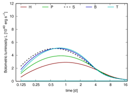
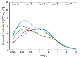
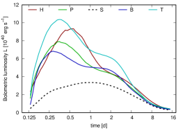
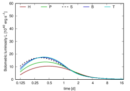
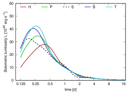
Figure 14: Angle-integrated bolometric luminosity as a function of time for the single-component morphologies. The top and bottom rows represent different compositions: low-$Y_{e}$ lanthanide-rich solar r-process residuals (top) vs high-$Y_{e}$ composition (bottom). Left column: uniform gray opacities (10 and 1 ${\rm cm}^{2}\,{\rm g}^{-1}$ for the top and bottom panels, respectively) Middle column: simulations using detailed opacities. Right column: bolometric luminosity estimate based on the temperature and the area of the outer surface (see Eq. B1). All models have mass $m_{\rm ej}=0.01\;M_{\odot}$, median expansion velocity $v_{\rm ej}=0.2\;c$ and uniform analytic power-law heating (without thermalization). The labels on the right panel show the area of the outer surface for the morphologies relative to the spherical model.

One way to understand the features of the kilonova light curves is to break it up into components. In this appendix, we study how the light curve of a single-component morphology is influenced by different factors, such as area of the photosphere or the temperature of the radiative layer. We apply phenomenological analysis of the radiative structure of axisymmetric morphologies and disentangle effects of geometry, density and opacity. For all models in this section, we assume uniform specific heating given by $\dot{\varepsilon}(t)=2\times 10^{10}\ t_{d}^{-1.3}\,\textrm{erg}\ \textrm{g}^{-1}\textrm{s}^{-1}$, where $t_{d}$ is the time since merger, in days (Metzger et al., 2010; Korobkin et al., 2012).

B.1 Gray-opacity models

In the gray-opacity approximation, models with more mass distributed at low optical depth are expected to be brighter. This is illustrated in Figure 14 (left column). Total luminosity can be estimated then using a simple expression:

$$L_{\rm gray}(t)=\dot{\varepsilon}(t)\,m_{\rm unc}(t),$$ (B1)

where $\dot{\varepsilon}(t)$ is the specific volumetric heating rate, and $m_{\rm unc}(t)$ is the “uncovered” mass, or the mass of the layer above the diffusion surface. The latter is defined as a surface at which the diffusion velocity $v_{\rm diff}=c/\tau$ equals the velocity differential to the edge of ejecta. Diffusion surface separates the bulk where photons are trapped from the outer envelope from where photons can escape, diffusing faster than the matter is expanding. Here, $\tau$ is the optical depth. In every (co-moving) point of homologously expanding ejecta with uniform gray opacity, $\tau(t)\propto t^{-2}$ (Grossman et al., 2014). This model has limited applicability: it does not take into account thermalization in the thin optical region above the photosphere and thus overestimates luminosity after the peak is reached.

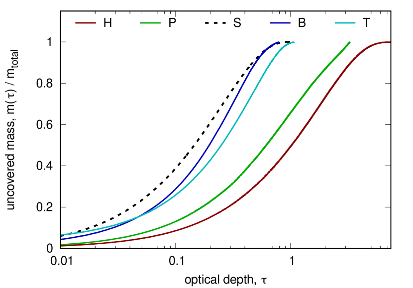
Figure 15: Fraction of mass uncovered above certain optical depth for models H, P, S, B, and T. Gray opacity ${\kappa=1\,{\rm cm}^{2}\,{\rm g}^{-1}}$ was used. The models are constrained to have the same total mass and average (RMS) expansion velocity.

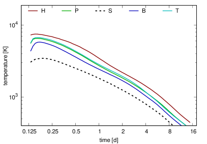
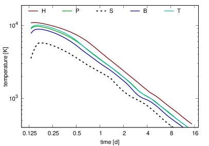
Figure 16: Radiation temperature at the matter boundary for the low-$Y_{e}$ (left) and high-$Y_{e}$ (right) compositions with analytic heating prescription.

Figure 16 shows the fraction of uncovered mass as a function of optical depth for axisymmetric morphologies, normalized to the same mass and rms expansion velocity. This profile $m_{\rm unc}(\tau)$ is only dependent on the density distribution inside each morphology, and is sufficient to estimate the bolometric light curve—using expression (B1) and the fact that $\tau(t)\propto t^{-2}$. If more mass is “buried” at high optical depth, the kilonova will peak later and be dimmer. Looking at Figure 16, we can anticipate that model S will peak earliest, followed by models B and T, and the models P and H will peak last. A similar trend is expected for the peak luminosity (in decreasing order). This is indeed observed in simulations with gray opacity in Figure 14 (left column), both for opacity $\kappa=10$ and $\kappa=1$.

B.2 Thin-layer models

When detailed opacities are introduced, their temperature dependence complicates the light curves, shifting peak time and luminosity by a factor of a few (Fig. 14, middle column). To understand these effects, we constructed a simple thin-layer approximation that uses snapshots of radiation temperature recorded by SuperNu during our simulations. Bolometric luminosity is computed as follows:

$$L_{\rm thin}(t)=A(t)\cdot c\ a\ T_{\rm out}^{4}(t),$$ (B2)

where $T_{\rm out}$ is the recorded temperature at the surface of the morphology (plotted in Figure 16), and $A(t)$ is the uniformly expanding area of this surface: $A(t)=A_{0}(t/t_{0})^{2}$. We use ${c\ a\ T_{\rm out}^{4}}$ for the surface flux instead of the usual $\sigma\ T_{\rm out}^{4}(\equiv{c\ a\ T_{\rm out}^{4}}/4)$ because in the thin photospheric layer, the radiation is free-streaming, such that intensity distribution is strongly peaked toward outward normal rather than being isotropic. In this case, the entire radiative energy in the bulk of photospheric layer is escaping. We also neglect photospheric recession and the corresponging decrease in the emitting area. Figure 7, which shows the fractional area of the diffusion surface (discussed in detail below), proves this to be a reasonable assumption, as for nonspherical morphologies, the area of diffusion surface remains at least 0.8 of the area of the outer contour for up to about 2 days. For the spherical morphology, this assumption is not very accurate and the “thin-layer” model is expected to overestimate the luminosity.

The resulting evolution of bolometric luminosity $L_{\rm thin}(t)$ is presented in the right column of Figure 14. Comparing it to the middle column on the same plot, we see that our model correctly reproduces the features of the bolometric light curves, but overestimates luminosities by about $20-40\%$. It also captures the order of peak times for different morphologies: B peaking first and H peaking the last. The same is only partly true for the order in peak brightness, as this approximation overestimates it for morphology H. Overall, our numerical experiment demonstrates that the features in the bolometric light curve are primarily dictated by the behavior of the surface temperature, and less so by the emitting area. In particular, spherical morphology S stands out by being the “coldest” and thus having the least luminous peak despite its having the largest surface area for the same mass and mean expansion velocity.

Next, we observe that the surface temperature ranking for different morphologies ($S<R<T\approx P<H$, Fig. 16) can be traced back to their ranking in density (Fig. 3). Naturally, models with higher density produce more radioactive heat per volume and are expected to be hotter. Moreover, if we compare bolometric luminosity of the low-$Y_{e}$ composition computed with thermalization taken into account (Fig. 9), it boosts the higher-density models even further, as more radioactive energy is thermalized in denser regions. Overall, density-dependent thermalization adds an extra boost by about factor of two in luminosity (cf. Fig. 9 and Fig. 14)

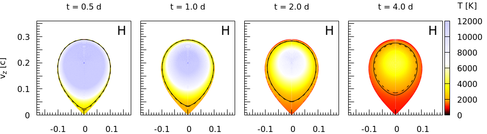
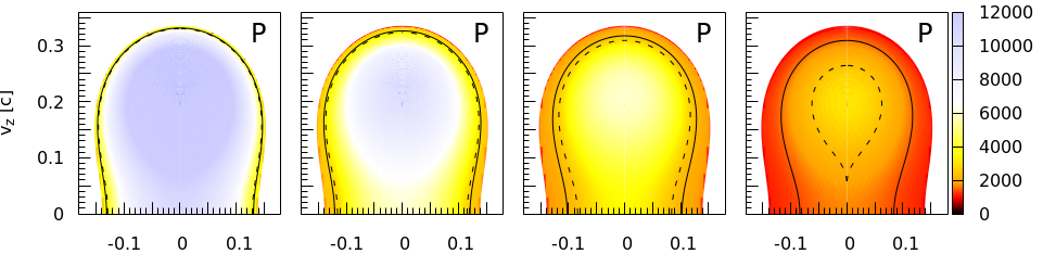
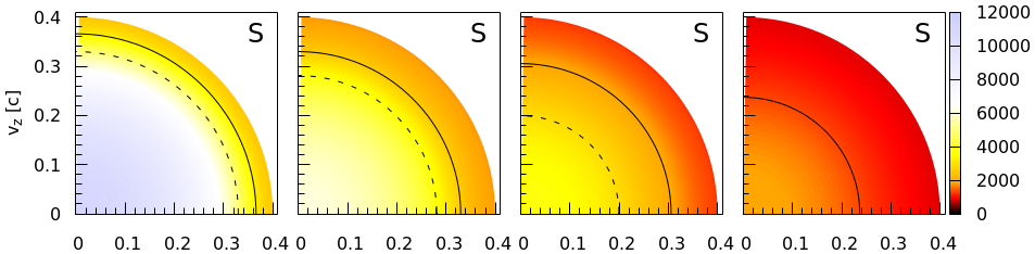
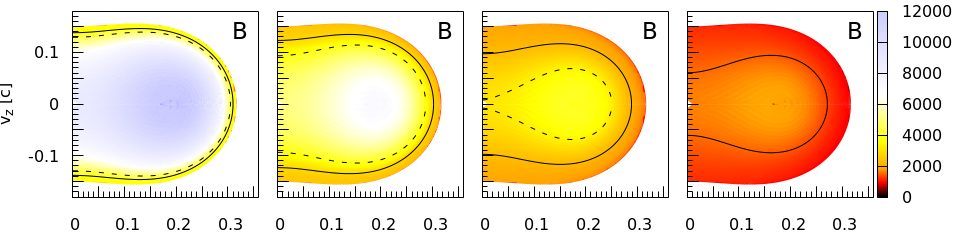
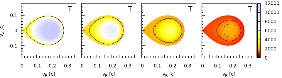
Figure 17: Temperature maps for axisymmetric single-component morphologies with solar r-process residuals for four different epochs. The black contours on each model mark the estimated locations of the diffusion surface (solid line) and the photosphere (dashed line).

The thin-layer model qualitatively reproduces the trends of the full radiative transfer model because it uses the surface temperatures from the simulations, which proves that the outbound Monte Carlo flux is consistent with the temperature evolution on the surface. Below we attempt to further validate the “thinness” assumption by explicitly calculating an approximate position of the diffusion surface from simulation data.

B.3 Estimating location of the diffusion surface and photosphere

Figure 17 shows the temperature color maps in our basic morphologies at different times, with overplotted estimated contours of the photosphere (dashed lines) and diffusion surface (solid lines). To locate the photosphere, we used Rosseland mean opacities and integrated the optical depth $d\tau=\kappa_{\rm R}(\rho,T)\rho d\ell$ inwards from the outer edge of the expansion, adjusting the path of integration so that it always follows the local density gradient. This results in a family of contours that determine the optical depth globally for every point as the optical depth minimized over all possible escape routes.

The photosphere is then given by the $\tau=2/3$ contour. It turns out, however, that the Rosseland mean significantly underestimates true effective opacity and places the photosphere too deep. Simple numerical integration of the radiative energy density in the layer above the photosphere computed in this manner gives numbers that greatly exceed the observed luminosity output of the kilonova.

A better way to pinpoint the location of the radiative layer is given by the diffusion surface. We define the diffusion surface as enclosing the opaque “core” of the ejecta where photons are escaping slower than local expansion and are therefore trapped (Grossman et al., 2014). To simplify the analysis, we make further approximations and compute the diffusion surface as given by an optical depth $\tau_{\rm ds}(t)$ such that the integral of the radiative energy $E_{\rm rad}$ above this contour ($\tau<\tau_{\rm ds}$) is equal to the total bolometric luminosity:

$$\int_{\tau<\tau_{\rm ds}(t)}E_{\rm rad}dV=L_{\rm bol}(t).$$ (B3)

This approximation ignores the anisotropy of radiation flux due to the asphericity of our models, but it is nevertheless sufficient to estimate the validity of the thin-layer approximation.

Indeed, Figure 17 allows us to conclude that for all morphologies except S, up to about 2 days the diffusion surface is not only very close to the outer edge of the expansion but also that the temperature in the radiative layer above it does not change significantly. So taking the surface temperature as a proxy for the thin-layer model is justified. On the other hand, contours of optical depth computed using the Rosseland mean fail to capture the photosphere: they instead place it inside the diffusion surface, which is unphysical for a typical kilonova scenario.

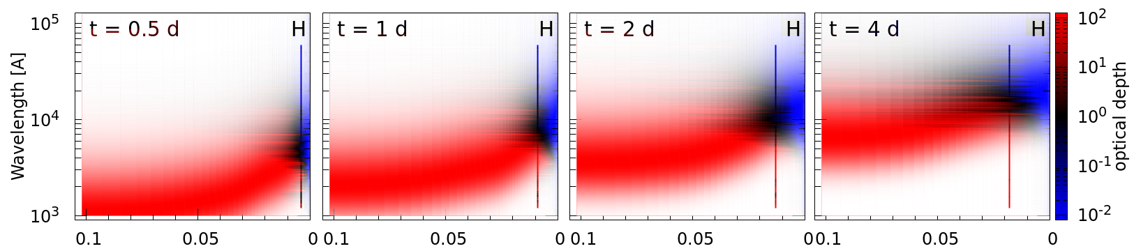
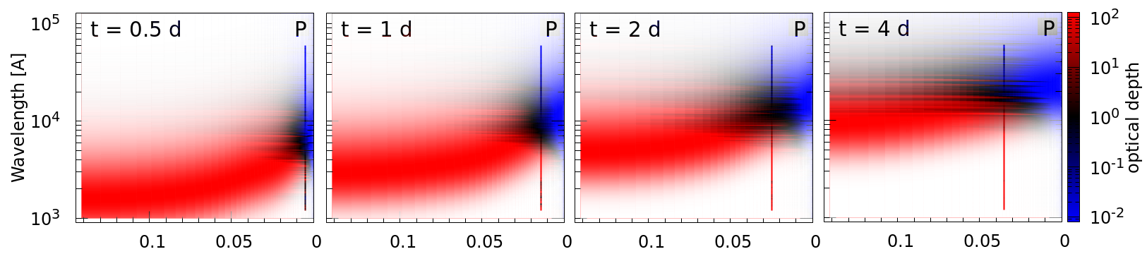
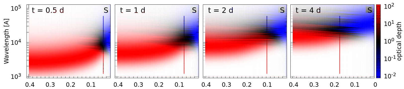
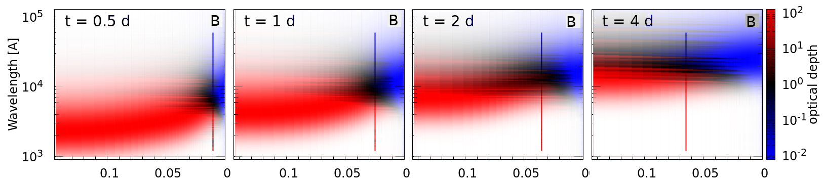
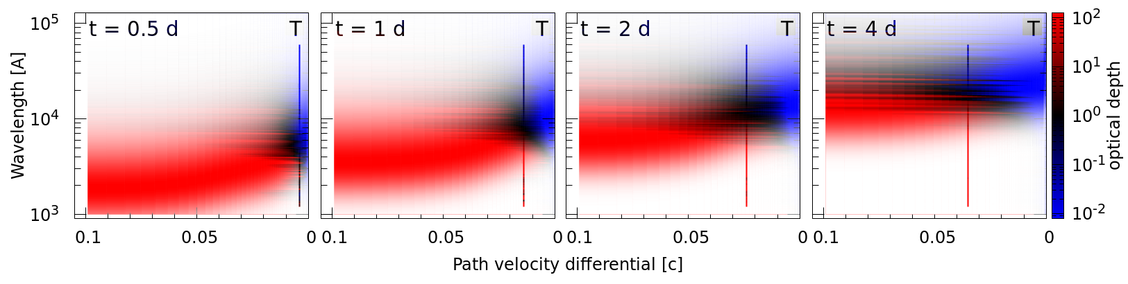
Figure 18: Wavelength-dependent optical depth for single-component morphologies with solar r-process residuals for four different epochs. The solid lines show locations of the diffusion surface. See the main text for a detailed description of the plot.

For any non-gray-opacity model, the location of the photosphere strongly depends on the wavelength. This point is clearly illustrated on Figure 18 (plots of this type were first introduced in Fontes et al., 2020). Each plot represents a color map of the wavelength-dependent optical depth experienced by a photon exiting the ejecta and moving out from an initial point along a given path. For the path, we picked a straight line starting from the density maximum orthogonal to the longer axis of the morphology. The horizontal axis starts at the density maximum and shows the overall velocity differential to the surface where the path terminates. Peaks and troughs in the opacity landscape generate streaks of optical depth that appear tilted down to the right due to the expansion redshift. As photons travel from left to right, they interact with progressively more redshifted opacity features, which creates the tilting effect. The opacity landscape also changes with depth due to the changes in density and temperature.

For nonspherical morphologies, photons traverse a velocity differential of only ${0.1\,c}$, while for spherical morphology (middle row), it is ${0.4\,c}$ and the “tilt” is much more noticeable.

The three-color heat map was selected to show three different regions in optical depth: low (blue), medium and comparable to the diffusion speed (black), and high (red). White matte regions on the plots are added to highlight the parts of the spectra where most of the photons would be emitted if spectra were blackbody. Transparency of the matte layer is proportional to the Planck function with the local radiation temperature. Solid vertical lines on each plot show the location of the diffusion surface.

The common feature on all plots is that the solid line crosses the optical depth map predominantly in the regions where the optical depth is “black,” i.e. $\sim 1-10$. In other words, the surface computed with Equation (B3) is located at an optical depth of about ${\tau_{\rm ds}\approx 10}$, which is where the diffusion surface should be for an outflow with an expansion velocity of ${c/10}$. This provides an additional argument in support of using line-binned opacities instead of expansion opacities for nonspherical models (see Fontes et al., 2020, for detailed exposition of the argument).

References

- Abbott et al. (2017a) Abbott B. P., et al., 2017a, Physical Review Letters, 119, 161101
- Abbott et al. (2017b) Abbott B. P., et al., 2017b, ApJ, 848, L12
- Abdikamalov et al. (2012) Abdikamalov E., Burrows A., Ott C. D., Löffler F., O’Connor E., Dolence J. C., Schnetter E., 2012, ApJ, 755, 111
- Baiotti & Rezzolla (2017) Baiotti L., Rezzolla L., 2017, Reports on Progress in Physics, 80, 096901
- Barbieri et al. (2019) Barbieri C., Salafia O. S., Perego A., Colpi M., Ghirlanda G., 2019, A&A, 625, A152
- Barnes & Kasen (2013) Barnes J., Kasen D., 2013, ApJ, 775, 18
- Barnes et al. (2016) Barnes J., Kasen D., Wu M.-R., Martínez-Pinedo G., 2016, ApJ, 829, 110
- Barnes et al. (2020) Barnes J., Zhu Y. L., Lund K. A., Sprouse T. M., Vassh N., McLaughlin G. C., Mumpower M. R., Surman R., 2020, arXiv e-prints, p. arXiv:2010.11182
- Bauswein et al. (2013) Bauswein A., Goriely S., Janka H. T., 2013, ApJ, 773, 78
- Bulla (2019) Bulla M., 2019, MNRAS, 489, 5037
- Castor & Lamers (1979) Castor J. I., Lamers H. J. G. L. M., 1979, ApJS, 39, 481
- Chornock et al. (2017) Chornock R., et al., 2017, ApJ, 848, L19
- Cleveland & Gentile (2014) Cleveland M. A., Gentile N., 2014, Journal of Computational and Theoretical Transport, 43, 6
- Côté et al. (2017) Côté B., Belczynski K., Fryer C. L., Ritter C., Paul A., Wehmeyer B., O’Shea B. W., 2017, ApJ, 836, 230
- Côté et al. (2018) Côté B., et al., 2018, ApJ, 855, 99
- Côté et al. (2019) Côté B., et al., 2019, ApJ, 875, 106
- Cowan et al. (2019) Cowan J. J., Sneden C., Lawler J. E., Aprahamian A., Wiescher M., Langanke K., Martínez-Pinedo G., Thielemann F.-K., 2019, arXiv e-prints, p. arXiv:1901.01410
- Cowperthwaite et al. (2017) Cowperthwaite P. S., et al., 2017, ApJ, 848, L17
- Darbha & Kasen (2020) Darbha S., Kasen D., 2020, ApJ, 897, 150
- De La Rosa et al. (2017) De La Rosa J., Roming P., Fryer C., 2017, ApJ, 850, 133
- Densmore et al. (2012) Densmore J. D., Thompson K. G., Urbatsch T. J., 2012, Journal of Computational Physics, 231, 6924
- Dietrich et al. (2017) Dietrich T., Bernuzzi S., Ujevic M., Tichy W., 2017, Phys. Rev. D, 95, 044045
- Eichler et al. (1989) Eichler D., Livio M., Piran T., Schramm D. N., 1989, Nature, 340, 126
- Evans et al. (2017) Evans P. A., et al., 2017, Science, 358, 1565
- Even et al. (2020) Even W., et al., 2020, ApJ, 899, 24
- Fahlman & Fernández (2018) Fahlman S., Fernández R., 2018, ApJ, 869, L3
- Fernández & Metzger (2013) Fernández R., Metzger B. D., 2013, MNRAS, 435, 502
- Fernández & Metzger (2016) Fernández R., Metzger B. D., 2016, Annual Review of Nuclear and Particle Science, 66, 23
- Fernández et al. (2015) Fernández R., Quataert E., Schwab J., Kasen D., Rosswog S., 2015, MNRAS, 449, 390
- Fleck Jr & Cummings Jr (1971) Fleck Jr J., Cummings Jr J., 1971, Journal of Computational Physics, 8, 313
- Fontes et al. (2015) Fontes C. J., Fryer C. L., Hungerford A. L., Hakel P., Colgan J., Kilcrease D. P., Sherrill M. E., 2015, High Energy Density Physics, 16, 53
- Fontes et al. (2017) Fontes C. J., Fryer C. L., Hungerford A. L., Wollaeger R. T., Rosswog S., Berger E., 2017, arXiv e-prints, p. arXiv:1702.02990
- Fontes et al. (2020) Fontes C. J., Fryer C. L., Hungerford A. L., Wollaeger R. T., Korobkin O., 2020, MNRAS, 493, 4143
- Freiburghaus et al. (1999) Freiburghaus C., Rosswog S., Thielemann F. K., 1999, ApJ, 525, L121
- Gaigalas et al. (2019) Gaigalas G., Kato D., Rynkun P., Radžiūtė L., Tanaka M., 2019, ApJS, 240, 29
- Goriely et al. (2011) Goriely S., Bauswein A., Janka H.-T., 2011, ApJ, 738, L32
- Grossman et al. (2014) Grossman D., Korobkin O., Rosswog S., Piran T., 2014, MNRAS, 439, 757
- Heinzel et al. (2021) Heinzel J., et al., 2021, MNRAS, 502, 3057
- Hotokezaka & Nakar (2019) Hotokezaka K., Nakar E., 2019, HeatingRate: Radioactive heating rate and macronova (kilonova) light curve (ascl:1911.008)
- Hotokezaka et al. (2015) Hotokezaka K., Piran T., Paul M., 2015, Nature Physics, 11, 1042
- Hotokezaka et al. (2018) Hotokezaka K., Beniamini P., Piran T., 2018, International Journal of Modern Physics D, 27, 1842005
- Janiuk (2014) Janiuk A., 2014, A&A, 568, A105
- Ji et al. (2019) Ji A. P., Drout M. R., Hansen T. T., 2019, ApJ, 882, 40
- Just et al. (2015) Just O., Bauswein A., Ardevol Pulpillo R., Goriely S., Janka H. T., 2015, MNRAS, 448, 541
- Kasen & Barnes (2019) Kasen D., Barnes J., 2019, ApJ, 876, 128
- Kasen et al. (2013) Kasen D., Badnell N. R., Barnes J., 2013, ApJ, 774, 25
- Kasen et al. (2015) Kasen D., Fernández R., Metzger B. D., 2015, MNRAS, 450, 1777
- Kasen et al. (2017) Kasen D., Metzger B., Barnes J., Quataert E., Ramirez-Ruiz E., 2017, Nature, 551, 80
- Kasliwal et al. (2017a) Kasliwal M. M., et al., 2017a, Science in press, available via doi:10.1126/science.aap9455,
- Kasliwal et al. (2017b) Kasliwal M. M., Korobkin O., Lau R. M., Wollaeger R., Fryer C. L., 2017b, ApJ, 843, L34
- Kawaguchi et al. (2018) Kawaguchi K., Shibata M., Tanaka M., 2018, ApJ, 865, L21
- Kawaguchi et al. (2020) Kawaguchi K., Shibata M., Tanaka M., 2020, ApJ, 889, 171
- Kilpatrick et al. (2017) Kilpatrick C. D., et al., 2017, Science in press, available via doi:10.1126/science.aaq0073,
- Kiuchi et al. (2017) Kiuchi K., Kawaguchi K., Kyutoku K., Sekiguchi Y., Shibata M., Taniguchi K., 2017, Phys. Rev. D, 96, 084060
- Korobkin et al. (2012) Korobkin O., Rosswog S., Arcones A., Winteler C., 2012, MNRAS, 426, 1940
- Kozyreva et al. (2017) Kozyreva A., et al., 2017, MNRAS, 464, 2854
- Krüger & Foucart (2020) Krüger C. J., Foucart F., 2020, Phys. Rev. D, 101, 103002
- Kyutoku et al. (2013) Kyutoku K., Ioka K., Shibata M., 2013, Phys. Rev. D, 88, 041503
- Lattimer & Schramm (1974) Lattimer J. M., Schramm D. N., 1974, ApJ, 192, L145
- Lippuner & Roberts (2015) Lippuner J., Roberts L. F., 2015, ApJ, 815, 82
- Martin et al. (2015) Martin D., Perego A., Arcones A., Thielemann F.-K., Korobkin O., Rosswog S., 2015, ApJ, 813, 2
- McCully et al. (2017) McCully C., et al., 2017, ApJ, 848, L32
- Metzger (2019) Metzger B. D., 2019, Living Reviews in Relativity, 23, 1
- Metzger et al. (2010) Metzger B. D., et al., 2010, MNRAS, 406, 2650
- Metzger et al. (2018) Metzger B. D., Thompson T. A., Quataert E., 2018, ApJ, 856, 101
- Miller et al. (2019) Miller J. M., et al., 2019, Phys. Rev. D, 100, 023008
- Nativi et al. (2020) Nativi L., Bulla M., Rosswog S., Lundman C., Kowal G., Gizzi D., Lamb G. P., Perego A., 2020, MNRAS,
- Oechslin et al. (2007) Oechslin R., Janka H.-T., Marek A., 2007, A&A, 467, 395
- Papenfort et al. (2018) Papenfort L. J., Gold R., Rezzolla L., 2018, Phys. Rev. D, 98, 104028
- Perego et al. (2014) Perego A., Rosswog S., Cabezón R. M., Korobkin O., Käppeli R., Arcones A., Liebendörfer M., 2014, MNRAS, 443, 3134
- Perego et al. (2017) Perego A., Radice D., Bernuzzi S., 2017, ApJ, 850, L37
- Pian et al. (2017) Pian E., et al., 2017, Nature, 551, 67
- Radice et al. (2016) Radice D., Galeazzi F., Lippuner J., Roberts L. F., Ott C. D., Rezzolla L., 2016, MNRAS, 460, 3255
- Radice et al. (2018) Radice D., Perego A., Hotokezaka K., Fromm S. A., Bernuzzi S., Roberts L. F., 2018, ApJ, 869, 130
- Roberts et al. (2011) Roberts L. F., Kasen D., Lee W. H., Ramirez-Ruiz E., 2011, ApJ, 736, L21
- Robinson (2007) Robinson K., 2007, The P Cygni Profile and Friends. Springer New York, New York, NY, pp 119–125, doi:10.1007/978-0-387-68288-4_10, https://doi.org/10.1007/978-0-387-68288-4_10
- Rosswog et al. (1998) Rosswog S., Thielemann F. K., Davies M. B., Benz W., Piran T., 1998, in Hillebrandt W., Muller E., eds, Nuclear Astrophysics. Springer New York, p. 103 (arXiv:astro-ph/9804332)
- Rosswog et al. (1999) Rosswog S., Liebendörfer M., Thielemann F. K., Davies M. B., Benz W., Piran T., 1999, A&A, 341, 499
- Rosswog et al. (2014) Rosswog S., Korobkin O., Arcones A., Thielemann F. K., Piran T., 2014, MNRAS, 439, 744
- Rosswog et al. (2017) Rosswog S., Feindt U., Korobkin O., Wu M.-R., Sollerman J., Goobar A., Martinez-Pinedo G., 2017, Classical and Quantum Gravity, 34, 104001
- Rosswog et al. (2018) Rosswog S., Sollerman J., Feindt U., Goobar A., Korobkin O., Wollaeger R., Fremling C., Kasliwal M. M., 2018, A&A, 615, A132
- Sekiguchi et al. (2016) Sekiguchi Y., Kiuchi K., Kyutoku K., Shibata M., Taniguchi K., 2016, Phys. Rev. D, 93, 124046
- Shibata & Hotokezaka (2019) Shibata M., Hotokezaka K., 2019, Annual Review of Nuclear and Particle Science, 69, annurev
- Shibata et al. (2017) Shibata M., Fujibayashi S., Hotokezaka K., Kiuchi K., Kyutoku K., Sekiguchi Y., Tanaka M., 2017, Phys. Rev. D, 96, 123012
- Siegel & Metzger (2018) Siegel D. M., Metzger B. D., 2018, ApJ, 858, 52
- Smartt et al. (2017) Smartt S. J., et al., 2017, Nature, 551, 75
- Smith et al. (2018) Smith A., Tsang B. T. H., Bromm V., Milosavljević M., 2018, MNRAS, 479, 2065
- Tanaka & Hotokezaka (2013) Tanaka M., Hotokezaka K., 2013, ApJ, 775, 113
- Tanaka et al. (2017) Tanaka M., et al., 2017, PASJ,
- Tanaka et al. (2020) Tanaka M., Kato D., Gaigalas G., Kawaguchi K., 2020, MNRAS, 496, 1369
- Tanvir et al. (2017) Tanvir N. R., et al., 2017, ApJ, 848, L27
- Troja et al. (2017) Troja E., et al., 2017, Nature, 551, 71
- Villar et al. (2017) Villar V. A., et al., 2017, ApJ, 851, L21
- Wallner et al. (2015) Wallner A., et al., 2015, Nature Communications, 6, 5956
- Wanajo et al. (2014) Wanajo S., Sekiguchi Y., Nishimura N., Kiuchi K., Kyutoku K., Shibata M., 2014, ApJ, 789, L39
- Wehmeyer et al. (2019) Wehmeyer B., Fröhlich C., Côté B., Pignatari M., Thielemann F. K., 2019, MNRAS, 487, 1745
- Winteler et al. (2012) Winteler C., Käppeli R., Perego A., Arcones A., Vasset N., Nishimura N., Liebendörfer M., Thielemann F. K., 2012, ApJ, 750, L22
- Wollaeger & van Rossum (2014) Wollaeger R. T., van Rossum D. R., 2014, The Astrophysical Journal Supplement Series, 214, 28
- Wollaeger et al. (2017) Wollaeger R. T., Hungerford A. L., Fryer C. L., Wollaber A. B., van Rossum D. R., Even W., 2017, ApJ, 845, 168
- Wollaeger et al. (2018) Wollaeger R. T., et al., 2018, MNRAS, 478, 3298
- Wollaeger et al. (2019) Wollaeger R. T., et al., 2019, ApJ, 880, 22
- Zhu et al. (2018) Zhu Y., et al., 2018, ApJ, 863, L23
- Zhu et al. (2019) Zhu Y., Barnes J., Lund K., Sprouse T., Vassh N., Mumpower M., McLaughlin G., Surman R., 2019, in APS Division of Nuclear Physics Meeting Abstracts. p. SM.003
- Zhu et al. (2020) Zhu J.-P., Yang Y.-P., Liu L.-D., Huang Y., Zhang B., Li Z., Yu Y.-W., Gao H., 2020, ApJ, 897, 20
- van Rossum et al. (2016) van Rossum D. R., Kashyap R., Fisher R., Wollaeger R. T., García-Berro E., Aznar-Siguán G., Ji S., Lorén-Aguilar P., 2016, ApJ, 827, 128