Possible link between the distribution of atomic spectral lines
and the radiation-matter-equilibrium in the early universe

Abstract

Abstract: We report on the uncanny resemblance of the global distribution of all experimentally known atomic spectral lines to the Planckian spectral distribution associated with black body radiation at a temperature of $T\approx 9000\,\mathrm{K}$. This value coincides with the critical temperature of equilibrium between the respective densities of radiation and matter in the early universe.

The characteristic spectral lines are commonly understood to be determined by the inner structure of an atom. As such, they constitute a direct outcome of quantum mechanics. Apart from higher-order corrections such as the Lamb shift, relativistic considerations therefore typically do not come up when the distribution of discrete electronic energy levels is discussed. In our work, we report on the observation that the global distribution of all experimentally known atomic spectral lines can be very accurately approximated by the Planckian function associated with a temperature of $T\approx 9,000\,\mathrm{K}$. As it happens, this value coincides with the critical temperature at which the respective densities of radiation density matter were in equilibrium in the early universe Gamov1948a ; Gamov1948b ; Alpher1948a ; Alpher1948b . Since we cannot present any explanation for our findings yet, this observation remains, for the moment, a striking conundrum. However, as so aptly stated by the late Isaac Asimov, “the most exciting phrase to hear in science, the one that heralds new discoveries, is not ‘Eureka!’ (I found it!) but ‘That’s funny…’ ”. In this spirit, we hope that an interested reader may possibly find a more satisfying explanation beyond the default assumption of a spurious correlation.

The first spectral lines were measured by William H. Wollaston and Joseph von Fraunhofer in 1802 and 1814, respectively Wollaston1802 ; Fraunhofer1814 . Initially, the presence of these features in the spectrum of the sun was a puzzle to the scientific community. Almost a whole century passed until Niels Bohr put forward his famous atomic model Bohr1913 as an explanation, which was later substantiated by Louis de Broglie deBroglie1924 . Today, using the Schrödinger equation Schrodinger1926 , atomic spectral lines (ASL) can be predicted with extremely high accuracy for numerous elements and their isotopes. Currently, more than 250,000 ASL are known and have been experimentally verified. The National Institute of Standards and Technology (NIST) manages an online catalogue wherein each of these lines is documented NIST and – barring complications such as government shutdowns – freely accessible. A global overview of this impressive data set is shown in Figure 1.

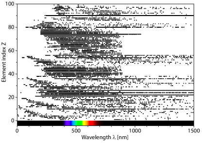
Figure 1: Overview of the known and experimentally verified spectral lines of neutral atoms up to $Z=100$ as listed in the NIST online catalogue NIST .

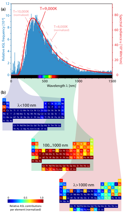
Figure 2: (a) Histogram of the relative frequency of all experimentally verified atomic spectral lines with a bin size of $5\,\textrm{nm}$ (blue bars). Its envelope closely traces the shape of the Planck distribution of the spectral radiance associated with a black body at the temperature $T=9,000\,\textrm{K}$ (solid red line) with its peak position of $\lambda=320\,\textrm{nm}$. The Planck distributions for $T=8,000\,\textrm{K}$ and $T=10,000\,\textrm{K}$, each normalized to the same peak height, are shown as dashed red lines and highlight the best match at $9,000\,\textrm{K}$.
(b) Color-coded relative contributions to the number of atomic spectral lines from each element in the extreme ultraviolet ($\lambda<100\,\mathrm{nm}$), between $100\,\mathrm{nm}$ and $1000\,\mathrm{nm}$, as well as the long infrared tail ($\lambda>1000\,\mathrm{nm}$). While outliers at short wavelengths predominantly stem from only two elements (${}_{19}\mathrm{K}$ Potassium and ${}_{11}\mathrm{Na}$ Sodium), the long-wavelength tail of the histogram mainly comprises lines from main-group elements. Notably, elements from across the entire periodic table contribute evenly to the Planck-like shape of the histogram, which therefore does not seem to be the result of inadvertent selection bias.

At first glance, the ASL of the different elements appear to be essentially randomly distributed. For some element numbers, a vast number of lines are known (e.g. $13,387$ for ${}_{90}\mathrm{Th}$ Thorium), for others only a few (two for ${}_{85}\mathrm{At}$ Astatine). Clearly, natural abundance and stability are only some of the factors determining the number of known lines for a given element, and a certain selection bias informed by the degree of technological relevance is likely to be at play. However, aside from these outliers, the overall size of the database all but ensures a fair sampling across the periodic table. Whereas the specific wavelengths, at which ASL can be found, vary greatly across the board, it is evident that their overwhelming majority falls in the band between $100\,\textrm{nm}\lesssim\lambda\lesssim 1000\,\textrm{nm}$.

This becomes even more obvious from a spectral histogram of the relative frequency (in the statistical sense) of the ASL, which is shown in Fig. 2(a). Here, the data presented in Fig. 1 is aggregated with a bin size of $5\,\textrm{nm}$. Only a small fraction of ASL occurs at very small wavelengths in or below the extreme ultraviolet regime ($\lambda\lesssim 100\,\mathrm{nm}$). The distribution peaks around $\lambda\approx 320\,\textrm{nm}$, whereas for higher wavelengths, the relative frequency decreases once more. Altogether, the distribution of the spectral lines’ relative frequency bears a striking similarity to the Planck distribution $u(\lambda)$ that describes the radiation energy density per wavelength unit emitted by a black body Planck1901

$$u(\lambda)=\frac{2\pi hc^{2}}{\lambda^{5}}\frac{1}{e^{\frac{hc}{\lambda k_{B}T}}-1}\,,$$ (1)

where $c$, $h$ and $k_{B}$ are the vacuum speed of light, Planck’s constant and the Boltzmann constant, respectively. As is well known, the peak position of this distribution is measure of the black body temperature $T$ Wien1893 . A best match to our histogram of known ASL is obtained for a temperature of $T\approx 9,000\,\textrm{K}$; the corresponding graph is plotted as red solid line in Fig. 2(a). While the match is particularly evident in the visible regime, small deviations occur at small and very large wavelengths. Nevertheless, the histogram of known ASL appears to be extraordinarily well described by radiation emitted by a black body of a temperature of $9,000\,\textrm{K}$.

At its face, the similarity between the ASL histogram and the Planck distribution is entirely unexpected and may appear entirely coincidental, since the continuous spectrum of thermal black-body radiation is the antithesis of the discrete energy quanta associated with atomic spectra. Moreover, apart from their common root within classical quantum theory, the ASL of different elements share no obvious connection to one another that would explain their collective overall distribution. Nevertheless, in the proverbial bird’s eye view enabled by the NIST database, their totality coalesces into the observed compact, continuous and distinctly shaped envelope. As shown in Figure 2(b), the entire periodic table contributes evenly to the bulk of the histogram, whereas outliers in the extreme UV predominantly stem from only two elements (${}_{19}\mathrm{K}$ Potassium and ${}_{11}\mathrm{Na}$ Sodium). Inadvertent selection effects of the aforementioned discrepancies in the number of known ASL for individual elements therefore do not lend themselves as convenient explanation for the observed similarity. As we will outline in the following, the seemingly arbitrary “temperature” of $9000\,\mathrm{K}$ – notably the only degree of freedom in Eq.(1) – may suggest a startling connection to cosmology.

Soon after Albert Einstein presented the fundamental concepts for general relativity in 1916 Einstein1916 , Alexander Friedmann derived his famous equation governing the dynamics of a homogeneous, isotropic universe Friedmann1922 :

$$\left(\frac{\dot{a}}{a}\right)^{2}=\frac{8\pi G}{3}\rho(t)-\frac{kc}{a^{2}}+\frac{1}{3}\Lambda\;,$$ (2)

where $G$ denotes the gravitational constant, $\Lambda$ represents the cosmological constant, $k$ is a constant relating to the curvature, and $a$ is the scale factor of the universe, essentially describing its size. From this equation, he was able to derive the energy-continuity equation

$$\dot{\rho}=-3\left(\rho+p\right)\frac{\dot{a}}{a}\;,$$ (3)

which connects pressure $p$ and energy density $\rho$. On these grounds, he considered two possible extreme situations: The first is a universe dominated by matter, such that $p=0$ and, consequently,

$$\rho_{\textrm{mat}}\varpropto a^{-3}\;.$$ (4)

The second is a universe dominated by radiation, such that $p=\rho/3$ and, consequently,

$$\rho_{\textrm{rad}}\varpropto a^{-4}\;.$$ (5)

Although today our universe is evidently matter-dominated, due to the different scaling of the two terms there must have been a time when $\rho_{\textrm{mat}}=\rho_{\textrm{rad}}$. Using Eq. 2, one can show that this transition occurred at a quite young age of the universe, approximately $50,000$ years after the big bang Carroll2007 . As it turns out, this phase transition took place when the temperature of the universe was approximately $T\approx 9,000\,\textrm{K}$ Gamov1948a ; Gamov1948b ; Alpher1948a ; Alpher1948b .

Setting aside the distinct possibility of a spurious correlation for the moment, a possible interpretation would be that this phase transition in the early universe may have played a previously unknown role in the formation of matter. However, the fundamental characteristics of elementary particles that determine the electromagnetic properties of the elements were already in place at this point. Avoiding the pitfalls of the post hoc fallacy logicalfallacy , a yet-to-be-discovered, deeper causal linkage may have left its fingerprints both in the distribution of atomic spectral lines across the elements of the periodic table, as well as the energy-matter balance of the universe as a whole. While we currently cannot offer a physical explanation to our entirely heuristic findings, it is our hope that they may inspire future work that could eventually lead to the resolution of this fascinating puzzle.

Methods

The NIST Atomic Spectra Database provides a comprehensive list of all experimentally verified spectral lines and line energies NIST . We retrieved this data with a self-written program TimsProgramm and evaluated the number of ASL in wavelength intervals of $5\,\textrm{nm}$. Notably, as long as dramatic oversampling is avoided, the specific window size neither has a systematic impact on the shape of the distribution, nor the on the temperature associated with the best-match black body spectrum.

The relative ASL contributions depicted in Figure 2(b) were determined by calculating the fraction of known spectral lines of a given element that fall in the spectral range under consideration. For example, of the 214 lines listed for ${}_{1}\mathrm{H}$ Hydrogen, 37 fall below $100\,\mathrm{nm}$ ($17.3\%$), 91 in the range between $100...1000\,\mathrm{nm}$ ($42.5\%$), and the remaining 86 lines ($40.2\%$) above $1000\,\mathrm{nm}$. In calculating these relative contributions, we were able to meaningfully compare the impact of elements with hugely disparate numbers of known lines.

In our statistical analysis, we focused on the spectral lines of neutral atoms, since each successive step of ionization necessarily excludes an element from the statistics and therefore over-emphasize the impact of higher elements. In a similar vein, each remaining electron in a given ion experiences a systematically deeper potential well, as the nuclear charge is less shielded, resulting in the histogram of spectral lines being shifted towards lower wavelengths (see Figure 3). Finally, the available spectral data becomes increasingly sparse with higher ionization numbers, effectively omitting large swaths of the ion triangle. In light of these considerations, we decided against the inclusion of ionic spectral lines.

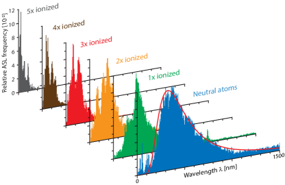
Figure 3: Histograms for ionic spectral lines. Each panel corresponds to an ionization step. The effectively larger nuclear charge of ions shifts their spectra towards shorter wavelengths. At the same time, the increasing sparsity of the data set yields more jagged histograms. To avoid these systematic and stochastic distortions, we excluded ionic spectral lines from our statistical analysis.

References

I Author contributions

T.R. conceived the idea, retrieved and processed the data. T.R., M.H., M.G. and A.S. discussed and interpreted the results. M.H. and M.G. prepared the figures. A.S. and M.H. wrote the manuscript.

II Competing financial interests

Competing interests, financial or otherwise, do not exist.

References

- (1) G. Gamov, “The Origin of Elements and the Separation of Galaxies,” Phys. Rev. 74, 505 (1948).
- (2) G. Gamov, “The Evolution of the Universe,” Nature 162, 680-682 (1948).
- (3) R. Alpher and R. Herman, “Comment on: The Evolution of the Universe,” Nature 162, 774-775 (1948).
- (4) R. Alpher and R. Herman, “On the Relative Abundance of the Elements,” Phys. Rev. 74, 1737-1742 (1948).
- (5) W. H. Wollaston, “A method of examining refractive and dispersive powers, by prismatic reflection,” Phil. Trans. R. Soc. 92, 365–380 (1802).
- (6) J. Fraunhofer, “Determination of the refractive and color-dispersing power of different types of glass, in relation to the improvement of achromatic telescopes,” Memoirs of the Royal Academy of Sciences in Munich 5, 193-226 (1814).
- (7) N. Bohr, “On the Constitution of Atoms and Molecules, Part I,” Philos. Mag. 26, 1-24 (1913).
- (8) L. de Broglie, “Recherches sur la theorie des quanta,” Ann. de Phys., 10e série, t. III (1925).
- (9) E. Schrödinger, “An Undulatory Theory of the Mechanics of Atoms and Molecules,” Phys. Rev. 28, 1049-1070 (1926).
- (10) http://physics.nist.gov/cgi-bin/ASD/lines_pt.pl
- (11) M. Planck, “Über das Gesetz der Energieverteilung im Normalspektrum,” Annal. Phys. 4, 553-563 (1901).
- (12) W. Wien, “Eine neue Beziehung der Strahlung schwarzer Körper zum zweiten Hauptsatz der Wärmetheorie,” Sitzungsberichte der Königlich Preußischen Akademie der Wissenschaften zu Berlin, Verl. d. Kgl. Akad. d. Wiss. S. 55 (1893).
- (13) A. Einstein, “Die Grundlage der allgemeinen Relativitätstheorie,” Annal. Phys. 354, 769-822 (1916).
- (14) A. Friedmann, “Über die Krümmung des Raumes,” Z. Phys. 10, 377-386 (1922).
- (15) B. Carroll and D. Ostlie, “An Introduction to Modern Astrophysics,” 2nd Ed., Pearson Eduction, Inc. (2007).
- (16) T. E. Damer, “Attacking Faulty Reasoning: A Practical Guide to Fallacy-Free Arguments,” (3rd ed.), Wadsworth Publishing, p. 131 (1995).
- (17) https://github.com/timrichardt/fetch-nist-asd