Clustering of Arrivals in Queueing Systems:
Autoregressive Conditional Duration Approach

March 17, 2024

Abstract: Arrivals in queueing systems are typically assumed to be independent and exponentially distributed. Our analysis of an online bookshop, however, shows that there is an autocorrelation structure present. First, we adjust the inter-arrival times for diurnal and seasonal patterns. Second, we model adjusted inter-arrival times by the generalized autoregressive score (GAS) model based on the generalized gamma distribution in the spirit of the autoregressive conditional duration (ACD) models. Third, in a simulation study, we investigate the effects of the dynamic arrival model on the number of customers, the busy period, and the response time in queueing systems with single and multiple servers. We find that ignoring the autocorrelation structure leads to significantly underestimated performance measures and consequently suboptimal decisions. The proposed approach serves as a general methodology for the treatment of arrivals clustering in practice.

Keywords: Inter-Arrival Times, Queueing Theory, Autoregressive Conditional Duration Model, Generalized Autoregressive Score Model, Retail Business.

JEL Codes: C41, C44, M11.

1 Introduction

In various applications of the operations research, it is undeniable that the characteristics of models evolve over time. The parameters of interest can depend on the time of day and season (see e.g. Kayacı Çodur and Yılmaz, 2020) as well as on their past values and other past indicators (see e.g. Bruzda, 2020). In the paper, we focus on the latter dependency in arrivals to queueing systems from the perspective of the autoregressive conditional duration models with the generalized autoregressive score dynamics.

Many standard queueing systems consider inter-arrival times to be independent due to analytical tractability. Some studies, however, explicitly consider autocorrelation and model arrivals using the Markovian arrival process (MAP) (see e.g. Adan and Kulkarni, 2003; Buchholz and Kriege, 2017; Manafzadeh Dizbin and Tan, 2019), the Markov renewal process (see e.g. Tin, 1985; Patuwo et al., 1993; Szekli et al., 1994), the moving average process (see e.g. Finch, 1963; Finch and Pearce, 1965; Pearce, 1967) or the discrete autoregressive process (see e.g. Hwang and Sohraby, 2003; Kamoun, 2006; Miao and Lee, 2013). Hwang and Sohraby (2003) argue that the time series models with few parameters are more suitable in practice than the MAP models which might be overparameterized. Simulation studies investigating the autocorrelation in arrivals include Livny et al. (1993), Resnick and Samorodnitsky (1997), Altiok and Melamed (2001), Nielsen (2007) and Civelek et al. (2009). Overall, these studies show that ignoring the autocorrelation structure, if present, leads to biased performance measures in queueing systems.

The arrival processes are also extensively studied in the financial high-frequency literature. In this field, the duration analysis deals with the modeling of times between successive transactions (trade durations), times until the price reaches a certain level (price durations), and times until a certain volume is traded (volume durations). Typically, the autoregressive conditional duration (ACD) model of Engle and Russell (1998) is utilized. Its dynamics are analogous to the generalized autoregressive conditional heteroskedasticity (GARCH) model of Bollerslev (1986). In its basic version, the ACD model is based on the exponential distribution but many other distributions are considered in the literature as well. Notably, Lunde (1999) introduces the generalized gamma distribution to the ACD model. Bauwens et al. (2004) and Fernandes and Grammig (2005) find that the generalized gamma distribution is more adequate than the exponential, Weibull, and Burr distributions in financial applications. Hautsch (2003) further finds that the four-parameter generalized F distribution reduces to the three-parameter generalized gamma distribution in most cases of financial durations. For a survey of the financial duration analysis, see Pacurar (2008) and Saranjeet and Ramanathan (2018).

A modern approach to time series modeling is the general autoregressive score (GAS) model of Creal et al. (2013), also known as the dynamic conditional score (DCS) model by Harvey (2013). The GAS model is an observation-driven model providing a general framework for modeling of time-varying parameters of any underlying probability distribution. It captures the dynamics of time-varying parameters by the autoregressive term and the score of the conditional density function utilizing the shape of the density function. The theoretical properties of the GAS models together with their estimation by the maximum likelihood method are investigated e.g. by Blasques et al. (2014) and Blasques et al. (2018). The empirical performance of the GAS models is studied e.g. by Koopman et al. (2016) and Blazsek and Licht (2020). So far, there are over 200 papers devoted to numerous models belonging to the GAS family with various applications – see Lucas (2020) for a comprehensive list of publications.

The class of the ACD models and the class of the GAS models overlap. In the case of the exponential distribution, the ACD model is equivalent to the GAS model (see Creal et al., 2013). For more complex distributions, however, they tend to differ as the ACD models are driven by the lagged observation (or, when rewritten, the difference between the observation and the expected value) while the GAS models are driven by the lagged score. In general, the GAS models are very often superior when compared to alternatives (see e.g. Blazsek and Villatoro, 2015; Koopman et al., 2016; Chen and Xu, 2019; Gorgi et al., 2019; Harvey et al., 2019; Blazsek and Licht, 2020). Concerning GAS models for positive or non-negative values that are suitable for the duration analysis, Fonseca and Cribari-Neto (2018) utilize the Birnbaum–Saunders distribution, Blasques et al. (2020) utilize the zero-inflated negative binomial distribution as well as the generalized gamma distribution, and Harvey and Ito (2020) utilize the generalized beta distribution as well as the generalized gamma distribution.

In the paper, we put together these three cornerstones – the queueing theory, the duration analysis, and the GAS models – and demonstrate that they fit together perfectly. The literature already successfully incorporates the GAS models to the duration analysis as discussed above while the perspective from the queueing theory is our novel contribution. We analyze inter-arrival times between orders from an online Czech bookshop. First, we adjust arrivals for diurnal and seasonal patterns using the cubic spline. Next, we find that the adjusted inter-arrival times exhibit strong clustering behavior – short inter-arrival times are usually followed by short times. To capture this autocorrelation, we utilize the dynamic model based on the generalized gamma distribution with the GAS dynamics in the spirit of the ACD models. We confirm that the proposed specification is quite suitable for the observed data. Finally, we investigate the effects of the proposed arrivals model on queueing systems with single and multiple servers and exponential services. In a simulation study, we show that various performance measures – the number of customers in the system, the busy period of servers, and the response time – have higher mean and variance as well as heavier tails for the proposed dynamic arrivals model than for the standard static model. Furthermore, we illustrate how the misspecification of the arrivals model can lead to suboptimal decisions.

The rest of the paper is structured as follows. In Section 2, we present the model based on the generalized gamma distribution with the GAS dynamics for diurnally adjusted inter-arrival times. In Section 3, we show that real data of a retail store exhibit an autocorrelation structure that is well captured by our model. In Section 4, we investigate the impact of the proposed arrivals model on the performance measures using simulations. We conclude the paper in Section 5.

2 Dynamic Model for Arrivals

2.1 Diurnal and Seasonal Adjustment

Before we utilize the generalized autoregressive score (GAS) model to capture the autoregressive structure of inter-arrival times, we need to deal with diurnal, weekly, and monthly seasonality patterns. To model the non-linear behavior of the diurnal and seasonal patterns and to properly adjust the inter-arrival times, the cubic spline method is utilized. The cubic spline is a piecewise cubic polynomial with continuous derivatives up to the order two at each $k$-th fixed point called a knot, $k=1,\dots,K$. Bruce and Bruce (2017) point out that the cubic spline method is often a superior approach to the polynomial regression since the polynomial regression often leads to undesirable "wiggliness" in the regression equation.

To take into account the specifics of raw inter-arrival times $\left\{\tilde{y}_{i}\right\}_{i=1}^{n}$, we define the cubic spline with knots at $\left\{\xi_{k}\right\}_{k=1}^{K}$ as

$$\log\tilde{y}_{i}=\beta_{0}+\beta_{1}b_{1}(x_{i})+\beta_{2}b_{2}(x_{i})+\dots+\beta_{K+3}b_{K+3}(x_{i})+\gamma t_{i}+\varepsilon_{i},$$ (1)

where $\left\{\beta_{j}\right\}_{j=1}^{K+3}$ and $\gamma$ are parameters to be estimated, $\varepsilon_{i}$ is disturbance term, $t_{i}$ is the trend variable, $\left\{b_{j}\right\}_{j=1}^{K+3}$ are the basis functions, and $x_{i}$ is a time difference in minutes between the time-stamp of the $i$th observation and the beginning of the week (Monday 00:00) to which the $i$th observation belongs. Thus, $\left\{x_{i}\right\}_{i=1}^{n}$ is able to capture both diurnal and intra-week patterns. The basis functions are equal to (i) the variable $x_{i}$, $b_{1}(x_{i})=x_{i}$; (ii) its square, $b_{2}(x_{i})=x^{2}_{i}$; (iii) its cube, $b_{3}(x_{i})=x^{3}_{i}$; and (iv) truncated power functions, $b_{k+3}(x_{i})=\max\left\{0,(x_{i}-\xi_{k})^{3}\right\},k=1,\dots,K$. The trend variable $t_{i}$ is linear in time (not linear in observations), $t_{1}=0$ and $t_{i}=\sum_{j=1}^{i-1}\tilde{y}_{j}$ for $i=2,\dots,n$, to take into account the irregularly spaced observations. Moreover, the logarithmic transformation of $\tilde{y}$ ensures the non-negativity of adjusted inter-arrival times. Equidistant intervals are used for knots identification since intervals based on quantiles might lead to a too-small number of knots allocated to off-peak hours.

Regression parameters in (1) are estimated by the weighted least squares (WLS) method with weights being the inter-arrival times. The WLS naturally compensates for the possibility that during a particular time interval either a small number of long inter-arrival times or a higher number of shorter inter-arrival times is observed, i.e. the number of observed inter-arrival times within a time interval depends on the values of inter-arrival times themselves. Unlike the ordinary least squares, this approach properly weights the inter-arrival times during hours that exhibit a small median but a huge dispersion. Once the parameters are estimated, the diurnally and seasonally adjusted and detrended inter-arrival times $y_{i}$ are set to exponentiated residuals from regression (1).

2.2 Generalized Gamma Distribution

Next, we consider the adjusted inter-arrival times $y_{i}$ to follow the generalized gamma distribution. The generalized gamma distribution is a continuous probability distribution for non-negative variables proposed by Stacy (1962). It is a three-parameter generalization of the two-parameter gamma distribution and contains the exponential distribution and the Weibull distribution as special cases. The distribution has the scale parameter $\alpha$ and the shape parameters $\psi>0$ and $\varphi>0$. We use the parametrization allowing for arbitrary values of $\alpha$ which is quite suitable for modeling of its dynamics. The probability density function is

$$f(y|\alpha,\psi,\varphi)=\frac{1}{\Gamma\left(\psi\right)}\frac{\varphi}{e^{\alpha}}\left(\frac{y}{e^{\alpha}}\right)^{\psi\varphi-1}e^{-\left(\frac{y}{e^{\alpha}}\right)^{\varphi}}\qquad\text{for }y\in(0,\infty),$$ (2)

where $\Gamma\left(\cdot\right)$ is the gamma function. The expected value and variance is

$$\mathrm{E}[Y] =e^{\alpha}\frac{\Gamma\left(\psi+\varphi^{-1}\right)}{\Gamma\left(\psi\right)},$$ (3)

$$\mathrm{var}[Y] =e^{2\alpha}\frac{\Gamma\left(\psi+2\varphi^{-1}\right)}{\Gamma\left(\psi\right)}-\left(e^{\alpha}\frac{\Gamma\left(\psi+\varphi^{-1}\right)}{\Gamma\left(\psi\right)}\right)^{2}.$$

The score for the parameter $\alpha$ is

$$\nabla_{\alpha}(y,\alpha,\psi,\varphi)=\frac{\partial\log f(y|\alpha,\psi,\varphi)}{\partial\alpha}=\varphi\left(y^{\varphi}e^{-\varphi\alpha}-\psi\right)\qquad\text{for }y\in(0,\infty).$$ (4)

The Fisher information for the parameter $\alpha$ is

$$\mathcal{I}_{\alpha}(\alpha,\psi,\varphi)=\mathrm{E}\left[\nabla_{\alpha}(y,\alpha,\psi,\varphi)^{2}\middle|\alpha,\psi,\varphi\right]=\psi\varphi^{2}.$$ (5)

Note that the Fisher information for $\alpha$ is not dependent on $\alpha$ itself. Special cases of the generalized gamma distribution include the gamma distribution for $\varphi=1$, the Weibull distribution for $\psi=1$ and the exponential distribution for $\psi=1$ and $\varphi=1$. The generalized gamma distribution itself is contained in a larger family – the generalized F distribution with four parameters.

2.3 Generalized Autoregressive Score Dynamics

Finally, we consider the scale parameter to be time-varying. In the generalized autoregressive score (GAS) framework of Creal et al. (2013), the time-varying parameters are linearly dependent on their lagged values and the lagged values of the score of the conditional density. Typically, only the first lag is utilized. In our case, the parameter $\alpha_{i}$ follows recursion

$$\alpha_{i+1} =c+b\alpha_{i}+a\nabla_{\alpha}(y_{i},\alpha_{i},\psi,\varphi)$$ (6)

$$=c+b\alpha_{i}+a\varphi\left(y_{i}^{\varphi}e^{-\varphi\alpha_{i}}-\psi\right),$$

where $c$ is the constant parameter, $b$ is the autoregressive parameter, $a$ is the score parameter and $\nabla_{\alpha}(y_{i},\alpha_{i},\psi,\varphi)$ is the score defined in (4). In the GAS framework, the score can be scaled by the inverse of the Fisher information or the square of the inverse of the Fisher information. In our case, however, both scaling functions based on the Fisher information and the unit scaling as well lead to the same model as the Fisher information does not depend on $\alpha_{i}$. The score for time-varying parameter $\alpha_{i}$ is the gradient of the log-likelihood with respect to $\alpha_{i}$ and indicates how sensitive the log-likelihood is to parameter $\alpha_{i}$. In the GAS model, the score drives the time variation in parameter $\alpha_{i}$ based on the shape of the generalized gamma density function.

Let $\theta=(c,b,a,\psi,\varphi)$ denote the vector of parameters in the model. We can estimate $\theta$ straightforwardly by the maximum likelihood method. The log-likelihood function is given by

$$\ell(\theta)=\ln f(y_{0}|\alpha_{0},\psi,\varphi)+\sum_{i=1}^{n}\ln f(y_{i}|\alpha_{i},\psi,\varphi),$$ (7)

where $f(\cdot)$ is the generalized gamma density function given by (2). We deliberately set aside the first term as the time-varying parameter $\alpha_{i}$ needs to be initialized at $i=0$. We set the value of $\alpha_{0}$ to the long-term mean value $c/(1-b)$. Subsequent values of $\alpha_{i}$, $i=1,\ldots,n$, than follow recursion (6). Finally, the parameter estimates $\hat{\theta}$ are obtained by non-linear optimization problem

$$\hat{\theta}\in\max_{\theta}\ell(\theta).$$ (8)

3 Empirical Evidence

3.1 Data Overview and Preparation

The data sample is obtained from the database of an online bookshop with one brick-and-mortar location in Prague, Czechia. The data cover the period of June 8 – December 20, 2018, resulting in $28$ full weeks and $5\,753$ observations. The precision of the timestamp is one minute. Thus, zero inter-arrival times might occur in the data due to two or more orders that arrive within one minute. Since the generalized gamma distribution has strictly positive support, the zero inter-arrival times are set to a small positive number. Bauwens (2006) replaces the zero inter-arrival times with a value equal to the half of the minimal positive inter-arrival time and argued that this is a more correct approach than their discarding. Hence, all 81 zero inter-arrival times are set to 0.5 minutes accordingly.

3.2 Diurnal and Seasonal Patterns

The raw inter-arrival time median is 24 minutes and the mean is 49 minutes – more than double due to long inter-arrival times during nights (specifically hours between midnight and 9 AM, see Figure 1). Hours between 9 and 11 AM exhibit many short inter-arrival times and several very long inter-arrival times resulting in high dispersion (SD = 111.39). The rest of the rush hours (until 5 PM) shows a similar inter-arrival time median but much lower dispersion (SD = 35.98). Moreover, strong weekly and monthly seasonal patterns are observed. The highest order counts (and consequently lower inter-arrival time values) occur at the beginning of a week and decrease until Saturday, see Figure 2). On Sundays, order counts increase again and exhibit the highest dispersion. During the summer months, the order counts are rather low (resulting in higher inter-arrival time values) and linearly increase until December.

To obtain the diurnally and seasonally adjusted and detrended inter-arrival times, the regression equation (1) with a selected number of knots is estimated. In practice, the selection of a suitable number of knots is an empirically-driven task. Bearing in mind, that too large number of knots can result in overfitting (e.g. one knot for every hour results in too unnatural bumpy behavior), on the other hand, that too low number of knots can result in insufficient fit (e.g. one knot for every 2 hours does not capture the nonlinear behavior of data satisfactorily), and after a little experimenting, we select one knot for every 90 minutes which captures all important nonlinearities and does not indicate overfitting. Note that the weekly aggregation is utilized in (1) which results in the same daily seasonal component for Mondays, Tuesdays, etc. To ensure continuity between Sundays and Mondays, the sample is stacked three times consecutively and the adjusted inter-arrival times are computed based on the second sub-sample. Parameters are estimated by the WLS.

The fitted values are shown in Figure 1 and 2. Note that they do not coincide with the smooth cubic spline function due to a linear trend which makes the corresponding fitted line "saw-toothed". The diurnally and seasonally adjusted and detrended inter-arrival times are computed as the exponentiated residuals of estimated equation (1) and for convenience, they are standardized to have unit mean. Their values range from 0.002 to 11.23 minutes.

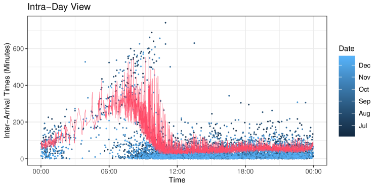
Figure 1: Intra-day view of raw inter-arrival times and their fitted diurnal/seasonal pattern.

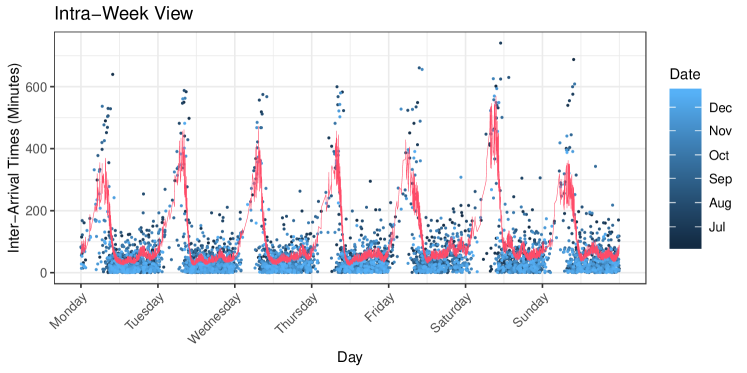
Figure 2: Intra-week view of raw inter-arrival times and their fitted diurnal/seasonal pattern.

3.3 Fit of the Dynamic Model

Even after the seasonal and diurnal adjustment, the inter-arrival times still tend to cluster over time – long (short) inter-arrival times are likely to be followed by long (short) inter-arrival times. This dependence is not particularly strong but nevertheless, it is statistically significant as illustrated in Figure 3. To capture the autocorrelation, we utilize the dynamic model based on the generalized gamma distribution with the GAS dynamics in (6). The parameters are estimated by the maximum likelihood method determined by the non-linear optimization problem in (8) and the log-likelihood function in (7). For comparison, we also report the results for static and dynamic models based on special cases of the generalized gamma distribution (G.G.), namely for the exponential (Exp.), Weibull and gamma distributions.

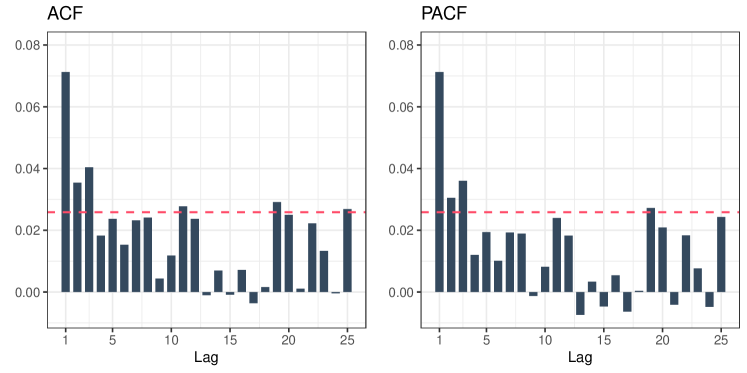
Figure 3: The autocorrelation function (ACF) and the partial autocorrelation function (PACF) of adjusted inter-arrival times. Red dashed lines indicate 5% confidence bounds.

Parameter estimates and the performance evaluation in terms of the Akaike information criterion (AIC) of both static and dynamic inter-arrival time models are shown in Table 1. The AIC values are at least by 43.59 lower for dynamic models than for their static counterparts. However, the differences among dynamic models are not so striking – the highest difference is between exponential and generalized gamma distributions (by 5.94). The best performing model is the most general one – the dynamic GAS model utilizing the generalized gamma distribution. The dynamic models based on either the exponential or generalized gamma distributions in comparison with their static counterparts are further analyzed in the simulation study of queueing systems.

Model		Estimate					Model Fit
Spec.	Dist.	$c$	$b$	$a$	$\psi$	$\varphi$	Lik.	AIC
Static	Exp.	0.00	0.00	0.00	1.00	1.00	$-5\,753.00$	$11\,508.00$
Static	Weibull	-0.01	0.00	0.00	1.00	0.97	$-5\,748.93$	$11\,501.86$
Static	Gamma	0.04	0.00	0.00	0.96	1.00	$-5\,749.77$	$11\,503.54$
Static	G. G.	-0.12	0.00	0.00	1.08	0.93	$-5\,748.37$	$11\,502.75$
Dyn.	Exp.	0.00	0.76	0.06	1.00	1.00	$-5\,728.28$	$11\,462.56$
Dyn.	Weibull	0.00	0.75	0.06	1.00	0.97	$-5\,724.89$	$11\,457.79$
Dyn.	Gamma	0.01	0.76	0.06	0.97	1.00	$-5\,725.97$	$11\,459.95$
Dyn.	G. G.	-0.06	0.72	0.07	1.15	0.90	$-5\,723.31$	$11\,456.62$

Table 1: Parameter estimates of the inter-arrival time models with the log-likelihood value (Lik.) and the Akaike information criterion (AIC).

4 Impact on Queueing Systems

4.1 System with Single Server

We investigate the effects of various arrival models on performance measures in queueing systems using simulations. We consider models based on the exponential and generalized gamma distributions with the static and dynamic specifications. The coefficients of the models are taken from Table 1. In all models, the rate of arrivals is $\lambda=1$ job per minute. First, we focus on the queueing system with a single server only. We consider the service times to be independent and exponentially distributed with the rate $\mu$ ranging from $1.1$ to $1.5$ jobs per minute. We simulate the arrival and service processes and measure the number of customers in the system, the busy period of the server, and the response time. The number of simulation runs is equal to $10^{9}$ which seems to be sufficient for the reported precision of one decimal place as the results are in line with the theoretical performance measures for the static exponential scenario as well as the Little’s law for all scenarios.

The results are reported in Table 2. For all values of $\mu$, the systems based on the generalized gamma distribution have higher values of performance measures than the systems based on the exponential distribution in terms of the mean, standard deviation, and $95$ percent quantile. Similarly, systems with the dynamic specification have higher values of performance measures than the systems with the static specification. The left plot of Figure 4 shows how the probability mass function of the number of customers differs for the static and dynamic models. The dynamic model has a higher probability of the empty system as there tend to be longer periods of low activity. It has also higher probabilities of large numbers of customers in the system as arrivals tend to cluster. The right plot of Figure 4 shows how the density function of the response time differs for the static and dynamic models. In the dynamic model, customers simply have to wait longer. The differences between the static and dynamic models are naturally weaker for larger $\mu$.

These results carry a warning for practice. When the standard M/M/1 system is assumed but the arrivals actually follow the GAS model based on the generalized gamma distribution, the performance measures are significantly underestimated. For example, the mean number of customers and the mean response time are $22$ percent lower than the actual value for $\mu=1.1$ jobs per minute. It is therefore crucial to correctly specify the model for arrivals.

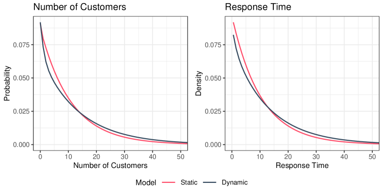
Figure 4: The probability mass functions of the number of customers in the system and density functions of the response time for the static and dynamic arrival models based on the generalized gamma distribution in the queueing system with single server and $\mu=1.1$ jobs per minute.

Queueing System			No. of Customers			Busy Period			Response Time
$\mu$	Spec.	Dist.	M	SD	95%	M	SD	95%	M	SD	95%
1.1	Static	Exp.	10.0	10.5	31.0	10.0	45.8	39.8	10.0	10.0	30.0
1.1	Static	G. G.	10.4	10.9	32.0	10.4	47.6	41.4	10.4	10.4	31.1
1.1	Dyn.	Exp.	12.4	13.4	39.0	10.8	54.4	41.2	12.4	12.6	37.6
1.1	Dyn.	G. G.	12.8	13.8	41.0	11.2	56.1	43.0	12.8	13.1	39.0
1.2	Static	Exp.	5.0	5.5	16.0	5.0	16.6	22.1	5.0	5.0	15.0
1.2	Static	G. G.	5.2	5.7	17.0	5.2	17.2	22.9	5.2	5.2	15.5
1.2	Dyn.	Exp.	6.0	6.8	20.0	5.4	19.5	23.3	6.0	6.1	18.3
1.2	Dyn.	G. G.	6.2	7.1	20.0	5.6	20.2	24.4	6.2	6.4	19.0
1.3	Static	Exp.	3.3	3.8	11.0	3.3	9.2	14.8	3.3	3.3	10.0
1.3	Static	G. G.	3.4	3.9	11.0	3.4	9.6	15.3	3.4	3.4	10.3
1.3	Dyn.	Exp.	3.9	4.6	13.0	3.5	10.7	15.7	3.9	4.0	11.9
1.3	Dyn.	G. G.	4.0	4.8	14.0	3.7	11.2	16.4	4.0	4.2	12.4
1.4	Static	Exp.	2.5	3.0	8.0	2.5	6.1	11.0	2.5	2.5	7.5
1.4	Static	G. G.	2.6	3.1	9.0	2.6	6.3	11.3	2.6	2.6	7.7
1.4	Dyn.	Exp.	2.8	3.5	10.0	2.6	7.0	11.5	2.8	2.9	8.7
1.4	Dyn.	G. G.	3.0	3.7	10.0	2.7	7.3	12.1	3.0	3.1	9.1
1.5	Static	Exp.	2.0	2.4	7.0	2.0	4.5	8.6	2.0	2.0	6.0
1.5	Static	G. G.	2.1	2.5	7.0	2.1	4.6	8.9	2.1	2.1	6.2
1.5	Dyn.	Exp.	2.2	2.9	8.0	2.1	5.1	9.0	2.2	2.3	6.8
1.5	Dyn.	G. G.	2.3	3.0	8.0	2.2	5.3	9.4	2.3	2.4	7.1

Table 2: Mean values (M), standard deviations (SD) and 95%-quantiles (95%) of the number of customers in the system, the busy period of the server and the response time in various queueing systems with a single server.

4.2 System with Multiple Servers

Next, we consider queueing systems with multiple servers. We base the simulations on the same setting as in the previous section. The only difference lies in the service structure. We consider the number of servers $c$ ranging from $11$ to $15$ with the individual service rate $\mu=0.1$ jobs per minute. Such values result in the same server utilizations $\rho=\lambda/(c\mu)$ as in the previous section. Again, we measure the number of customers in the system, the busy period of the servers, and the response time. By the busy period, we mean the full busy period, i.e. the duration of the state in which all servers are busy.

The results are reported in Table 3. The findings are very similar to the system with a single server – the generalized gamma distribution and the dynamic specification increase all performance measures. When incorrectly assuming the M/M/c system, the specification error is distinct but not as high as in the case of a single server. For example, when assuming the M/M/11 system, the mean number of customers and the mean response time are $14$ percent lower than the actual value for arrivals based on the generalized gamma distribution with the dynamic specification.

We illustrate how the misspecification of the arrival model can affect decision making in the following toy example. Let us consider that there are two types of costs associated with the operation of the system – the cost of running one server per unit of time $C_{1}=10$ euro per minute and the cost of the queue longer than $30$ customers per unit of time $C_{2}=$3\,000$$ euro per minute. The analytic department is faced with the question of how many servers to operate. The composition of costs for different numbers of servers is shown in Figure 5. The optimal number of servers according to the static model is $12$ while it is $13$ for the dynamic model. An analyst assuming the static model believes that the total optimal costs are $127.13$ euro per minute while they actually are $142.87$ euro per minute for the suboptimal choice of 12 servers. An analyst correctly specifying the dynamic model finds out that the lowest possible costs are $132.32$ euro per minute for the optimal choice of 13 servers. The decision based on the misspecified arrival model therefore results in a total cost increase of $8$ percent.

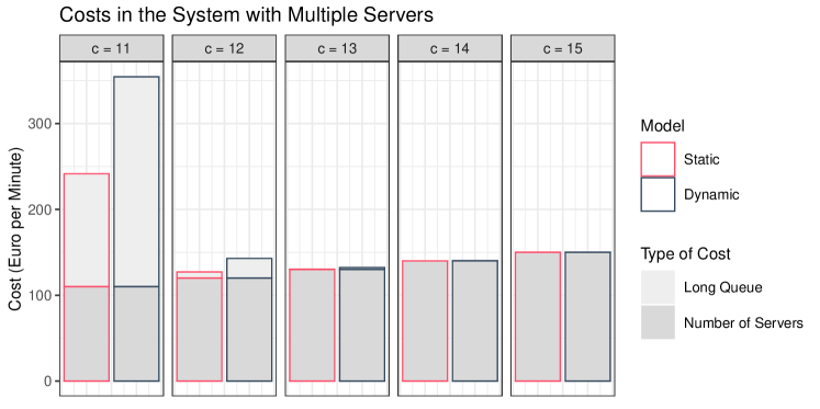
Figure 5: Costs related to the number of servers and long queue for the static and dynamic arrival models based on the generalized gamma distribution in the queueing systems with multiple servers and $\mu=0.10$ jobs per minute.

Queueing System			No. of Customers			Busy Period			Response Time
$c$	Spec.	Dist.	M	SD	95%	M	SD	95%	M	SD	95%
11	Static	Exp.	16.8	10.7	38.0	10.0	45.8	39.9	16.8	13.8	43.8
11	Static	G. G.	17.2	11.1	39.0	10.4	47.6	41.4	17.2	14.0	44.6
11	Dyn.	Exp.	19.1	13.5	46.0	12.4	58.6	49.7	19.1	15.7	49.9
11	Dyn.	G. G.	19.5	14.0	47.0	12.8	60.3	51.8	19.5	16.1	50.9
12	Static	Exp.	12.2	5.8	24.0	5.0	16.6	22.1	12.2	10.8	33.6
12	Static	G. G.	12.4	6.1	24.0	5.2	17.2	22.9	12.4	10.9	33.8
12	Dyn.	Exp.	13.1	7.2	27.0	6.1	21.1	27.5	13.1	11.3	35.4
12	Dyn.	G. G.	13.3	7.5	28.0	6.3	21.9	28.7	13.3	11.5	35.8
13	Static	Exp.	11.0	4.4	19.0	3.3	9.2	14.8	11.0	10.3	31.3
13	Static	G. G.	11.0	4.5	19.0	3.4	9.6	15.3	11.0	10.3	31.4
13	Dyn.	Exp.	11.4	5.2	21.0	4.0	11.7	18.4	11.4	10.5	32.0
13	Dyn.	G. G.	11.5	5.4	22.0	4.2	12.1	19.1	11.5	10.5	32.2
14	Static	Exp.	10.4	3.8	17.0	2.5	6.1	11.0	10.4	10.1	30.5
14	Static	G. G.	10.5	3.9	17.0	2.6	6.3	11.3	10.5	10.1	30.6
14	Dyn.	Exp.	10.7	4.4	19.0	3.0	7.7	13.5	10.7	10.2	30.9
14	Dyn.	G. G.	10.7	4.5	19.0	3.1	8.0	14.0	10.7	10.2	30.9
15	Static	Exp.	10.2	3.5	16.0	2.0	4.5	8.6	10.2	10.0	30.2
15	Static	G. G.	10.2	3.6	16.0	2.1	4.6	8.9	10.2	10.0	30.2
15	Dyn.	Exp.	10.3	3.9	17.0	2.3	5.6	10.5	10.3	10.1	30.4
15	Dyn.	G. G.	10.3	4.1	18.0	2.4	5.8	10.9	10.3	10.1	30.4

Table 3: Mean values (M), standard deviations (SD) and 95%-quantiles (95%) of the number of customers in the system, the full busy period of servers and the response time in various queueing systems with multiple servers and $\mu=0.1$ jobs per minute.

4.3 Discussion of More Complex Systems

In this paper, we focus on rather simple queueing systems in order to get transparent results. The M/M/1 system is as straightforward as it can be and therefore the best choice for an illustration of the impact of autocorrelated arrivals. The M/M/c system is used as a robustness check to show that the behavior observed for the M/M/1 system is present even for different specifications. As for the toy example of decision making in the M/M/c system, it is meant just as a simplistic illustration revealing a potential source of suboptimal decisions.

On the other hand, Tomanová (2018), Tomanová (2019a), and Tomanová (2019b) explore a much more realistic and complex queueing system specific to our online bookshop case. As this queueing system is tailored just for this specific application and cannot be easily transferred to others, we only summarize the main findings. Tomanová (2018) performs a process quality assessment based on process simulation and reports that the key quality target is not satisfied in almost twice more cases when the dynamic model is considered (the target is not satisfied in 6.16 percent) than when the static model is considered (for which the target is not satisfied in 3.23 percent). The common approach – a static model which assumes that times between arrivals follow the exponential distribution with a constant rate – underestimates the probability of extreme values and thus significantly skews the basis for process quality assessment and leads to suboptimal decisions. Tomanová (2019a) also demonstrates that the clustering of arrivals increases the probability of weeks with an extreme number of arrivals that has a negative impact on target fulfillment. Tomanová (2019b) further extends the work for final recommendations for the management of the online bookshop. The main finding is that 21 percent of orders are not satisfied within a working day due to insufficiently allocated resources for the first stage (pre-processing of arrivals).

5 Conclusion

We analyze the dependence of inter-arrival times in queueing systems and demonstrate the negative impact of arrival model misspecification on decision making. To capture the autocorrelation structure of inter-arrival times, we propose to utilize a dynamic model based on the generalized gamma distribution with the GAS dynamics. We argue that this approach is superior to the standard model assuming the exponential distribution with a constant rate since it leads to a more faithful representation of the mean and extreme values of the arrival process. Our approach consists of three steps.

1. We construct a suitable model for capturing the diurnal and seasonal dependencies which takes into account a specific time-structure of inter-arrival times. We utilize a cubic spline approach and propose to estimate the parameters by the weighted ordinary least square method to properly adjust inter-arrival times during hours that exhibit a small median but a huge dispersion.

2. We argue that the GAS models based on the generalized gamma distribution and its special cases fit the data better than their static counterparts. This is due to the fact that the static models ignore the autocorrelation structure which is still present even after the proper diurnal and seasonal adjustment.

3. We compare both static and dynamic models in the simulation study of queueing systems with single and multiple servers and exponential services. We show that ignoring the autocorrelation structure leads to biased performance measures. The number of customers in the system, the busy period of servers and the response time have higher mean and variance as well as heavier tails for the proposed dynamic arrivals model than for the standard static model. We also demonstrate how the trust in the standard static model for inter-arrival times leads to suboptimal decisions and consequently to a profit loss.

A proper treatment of arrival dependence is of a great importance since its ignorance generates extra costs. Our approach is useful for process simulations and consequently for process optimization and process quality assessment.

The main limitation of the paper and a topic for future research is the theoretical treatment of the queueing systems with inter-arrival times following the GAS model. In the paper, we resort to simulations to determine the moments, quantiles, and density functions of the performance measures. Theoretical derivation of these quantities and functions is undoubtedly challenging but perhaps possible in some cases. Another topic for future research, that is easier to achieve, is the use of the proposed approach in other applications. Besides retail order processing, these may include customer service, project management, manufacturing engineering, emergency services, logistics, transportation, telecommunication, computing, and others.

Funding

The work on this paper was supported by the Internal Grant Agency of the University of Economics, Prague under project F4/27/2020 and the Czech Science Foundation under project 19-08985S.

References

- Adan and Kulkarni (2003) Adan, I. J. B. F., Kulkarni, V. G. 2003. Single-Server Queue with Markov-Dependent Inter-Arrival and Service Times. Queueing Systems. Volume 45. Issue 2. Pages 113–134. ISSN 0257-0130. {https://doi.org/10.1023/a:1026093622185}.
- Altiok and Melamed (2001) Altiok, T., Melamed, B. 2001. The Case for Modeling Correlation in Manufacturing Systems. IIE Transactions. Volume 33. Issue 9. Pages 779–791. ISSN 0740-817X. {https://doi.org/10.1080/07408170108936872}.
- Bauwens (2006) Bauwens, L. 2006. Econometric Analysis of Intra-Daily Trading Activity on the Tokyo Stock Exchange. Monetary and Economic Studies. Volume 24. Issue 1. Pages 1–24. ISSN 0288-8432. {http://www.imes.boj.or.jp/research/abstracts/english/me24-1-1.html}.
- Bauwens et al. (2004) Bauwens, L., Giot, P., Grammig, J., Veredas, D. 2004. A Comparison of Financial Duration Models via Density Forecasts. International Journal of Forecasting. Volume 20. Issue 4. Pages 589–609. ISSN 0169-2070. {https://doi.org/10.1016/j.ijforecast.2003.09.014}.
- Blasques et al. (2014) Blasques, F., Koopman, S. J., Lucas, A. 2014. Stationarity and Ergodicity of Univariate Generalized Autoregressive Score Processes. Electronic Journal of Statistics. Volume 8. Issue 1. Pages 1088–1112. ISSN 1935-7524. {https://doi.org/10.1214/14-ejs924}.
- Blasques et al. (2018) Blasques, F., Gorgi, P., Koopman, S. J., Wintenberger, O. 2018. Feasible Invertibility Conditions and Maximum Likelihood Estimation for Observation-Driven Models. Electronic Journal of Statistics. Volume 12. Issue 1. Pages 1019–1052. ISSN 1935-7524. {https://doi.org/10.1214/18-ejs1416}.
- Blasques et al. (2020) Blasques, F., Holý, V., Tomanová, P. 2020. Zero-Inflated Autoregressive Conditional Duration Model for Discrete Trade Durations with Excessive Zeros. Working Paper. {https://arxiv.org/abs/1812.07318}.
- Blazsek and Licht (2020) Blazsek, S., Licht, A. 2020. Dynamic Conditional Score Models: A Review of Their Applications. Applied Economics. Volume 52. Issue 11. Pages 1181–1199. ISSN 0003-6846. {https://doi.org/10.1080/00036846.2019.1659498}.
- Blazsek and Villatoro (2015) Blazsek, S., Villatoro, M. 2015. Is Beta-t-EGARCH(1,1) Superior to GARCH(1,1)? Applied Economics. Volume 47. Issue 17. Pages 1764–1774. ISSN 0003-6846. {https://doi.org/10.1080/00036846.2014.1000536}.
- Bollerslev (1986) Bollerslev, T. 1986. Generalized Autoregressive Conditional Heteroskedasticity. Journal of Econometrics. Volume 31. Issue 3. Pages 307–327. ISSN 0304-4076. {https://doi.org/10.1016/0304-4076(86)90063-1}.
- Bruce and Bruce (2017) Bruce, P., Bruce, A. 2017. Practical Statistics for Data Scientists: 50 Essential Concepts. Sebastopol. O’Reilly Media. ISBN 978-1-4919-5295-5. {https://www.oreilly.com/library/view/practical-statistics-for/9781491952955/}.
- Bruzda (2020) Bruzda, J. 2020. Multistep Quantile Forecasts for Supply Chain and Logistics Operations: Bootstrapping, the GARCH Model and Quantile Regression Based Approaches. Central European Journal of Operations Research. Volume 28. Issue 1. Pages 309–336. ISSN 1435-246X. {https://doi.org/10.1007/s10100-018-0591-2}.
- Buchholz and Kriege (2017) Buchholz, P., Kriege, J. 2017. Fitting Correlated Arrival and Service Times and Related Queueing Performance. Queueing Systems. Volume 85. Issue 3-4. Pages 337–359. ISSN 0257-0130. {https://doi.org/10.1007/s11134-017-9514-5}.
- Chen and Xu (2019) Chen, R., Xu, J. 2019. Forecasting Volatility and Correlation Between Oil and Gold Prices Using a Novel Multivariate GAS Model. Energy Economics. Volume 78. Pages 379–391. ISSN 0140-9883. {https://doi.org/10.1016/j.eneco.2018.11.011}.
- Civelek et al. (2009) Civelek, I., Biller, B., Scheller-Wolf, A. 2009. The Impact of Dependence on Queueing Systems. Working Paper. {https://www.researchgate.net/publication/228814043}.
- Creal et al. (2013) Creal, D., Koopman, S. J., Lucas, A. 2013. Generalized Autoregressive Score Models with Applications. Journal of Applied Econometrics. Volume 28. Issue 5. Pages 777–795. ISSN 0883-7252. {https://doi.org/10.1002/jae.1279}.
- Engle and Russell (1998) Engle, R. F., Russell, J. R. 1998. Autoregressive Conditional Duration: A New Model for Irregularly Spaced Transaction Data. Econometrica. Volume 66. Issue 5. Pages 1127–1162. ISSN 0012-9682. {https://doi.org/10.2307/2999632}.
- Fernandes and Grammig (2005) Fernandes, M., Grammig, J. 2005. Nonparametric Specification Tests for Conditional Duration Models. Journal of Econometrics. Volume 127. Issue 1. Pages 35–68. ISSN 0304-4076. {https://doi.org/10.1016/j.jeconom.2004.06.003}.
- Finch (1963) Finch, P. D. 1963. The Single Server Queueing System with Non-Recurrent Input-Process and Erlang Service Time. Journal of the Australian Mathematical Society. Volume 3. Issue 2. Pages 220–236. ISSN 1446-8107. {https://doi.org/10.1017/s1446788700027968}.
- Finch and Pearce (1965) Finch, P. D., Pearce, C. 1965. A Second Look at a Queueing System with Moving Average Input Process. Journal of the Australian Mathematical Society. Volume 5. Issue 1. Pages 100–106. ISSN 1446-8107. {https://doi.org/10.1017/s144678870002591x}.
- Fonseca and Cribari-Neto (2018) Fonseca, R. V., Cribari-Neto, F. 2018. Bimodal Birnbaum-Saunders Generalized Autoregressive Score Model. Journal of Applied Statistics. Volume 45. Issue 14. Pages 2585–2606. ISSN 0266-4763. {https://doi.org/10.1080/02664763.2018.1428734}.
- Gorgi et al. (2019) Gorgi, Koopman, S. J., Lit, R. 2019. The Analysis and Forecasting of Tennis Matches by Using a High Dimensional Dynamic Model. Journal of the Royal Statistical Society: Series A (Statistics in Society). Volume 182. Issue 4. Pages 1393–1409. ISSN 0964-1998. {https://doi.org/10.1111/rssa.12464}.
- Harvey et al. (2019) Harvey, A., Hurn, S., Thiele, S. 2019. Modeling Directional (Circular) Time Series. Working Paper.
- Harvey (2013) Harvey, A. C. 2013. Dynamic Models for Volatility and Heavy Tails: With Applications to Financial and Economic Time Series. First Edition. New York. Cambridge University Press. ISBN 978-1-107-63002-4. {https://doi.org/0.1017/cbo9781139540933}.
- Harvey and Ito (2020) Harvey, A. C., Ito, R. 2020. Modeling Time Series When Some Observations Are Zero. Journal of Econometrics. Volume 214. Issue 1. Pages 33–45. ISSN 0304-4076. {https://doi.org/10.1016/j.jeconom.2019.05.003}.
- Hautsch (2003) Hautsch, N. 2003. Assessing the Risk of Liquidity Suppliers on the Basis of Excess Demand Intensities. Journal of Financial Econometrics. Volume 1. Issue 2. Pages 189–215. ISSN 1479-8409. {https://doi.org/10.1093/jjfinec/nbg010}.
- Hwang and Sohraby (2003) Hwang, G. U., Sohraby, K. 2003. On the Exact Analysis of a Discrete-Time Queueing System with Autoregressive Inputs. Queueing Systems. Volume 43. Issue 1-2. Pages 29–41. ISSN 0257-0130. {https://doi.org/10.1023/a:1021848330183}.
- Kamoun (2006) Kamoun, F. 2006. The Discrete-Time Queue with Autoregressive Inputs Revisited. Queueing Systems. Volume 54. Issue 3. Pages 185–192. ISSN 0257-0130. {https://doi.org/10.1007/s11134-006-9591-3}.
- Kayacı Çodur and Yılmaz (2020) Kayacı Çodur, M., Yılmaz, M. 2020. A Time-Dependent Hierarchical Chinese Postman Problem. Central European Journal of Operations Research. Volume 28. Issue 1. Pages 337–366. ISSN 1435-246X. {https://doi.org/10.1007/s10100-018-0598-8}.
- Koopman et al. (2016) Koopman, S. J., Lucas, A., Scharth, M. 2016. Predicting Time-Varying Parameters with Parameter-Driven and Observation-Driven Models. Review of Economics and Statistics. Volume 98. Issue 1. Pages 97–110. ISSN 0034-6535. {https://doi.org/10.1162/rest_a_00533}.
- Livny et al. (1993) Livny, M., Melamed, B., Tsiolis, A. K. 1993. The Impact of Autocorrelation on Queuing Systems. Management Science. Volume 39. Issue 3. Pages 322–339. ISSN 0025-1909. {https://doi.org/10.2307/2632647}.
- Lucas (2020) Lucas, A. 2020. Generalized Autoregressive Score Models. Online. {http://www.gasmodel.com}.
- Lunde (1999) Lunde, A. 1999. A Generalized Gamma Autoregressive Conditional Duration Model. Working Paper. {https://www.researchgate.net/publication/228464216}.
- Manafzadeh Dizbin and Tan (2019) Manafzadeh Dizbin, N., Tan, B. 2019. Modelling and Analysis of the Impact of Correlated Inter-Event Data on Production Control Using Markovian Arrival Processes. Flexible Services and Manufacturing Journal. Volume 31. Issue 4. Pages 1042–1076. ISSN 1936-6582. {https://doi.org/10.1007/s10696-018-9329-7}.
- Miao and Lee (2013) Miao, D. W. C., Lee, H. C. 2013. Second-Order Performance Analysis of Discrete-Time Queues Fed by DAR(2) Sources with a Focus on the Marginal Effect of the Additional Traffic Parameter. Applied Stochastic Models in Business and Industry. Volume 29. Issue 1. Pages 45–60. ISSN 1524-1904. {https://doi.org/10.1002/asmb.939}.
- Nielsen (2007) Nielsen, E. H. 2007. Autocorrelation in Queuing Network-Type Production Systems - Revisited. International Journal of Production Economics. Volume 110. Issue 1-2. Pages 138–146. ISSN 0925-5273. {https://doi.org/10.1016/j.ijpe.2007.02.014}.
- Pacurar (2008) Pacurar, M. 2008. Autoregressive Conditional Duration Models in Finance: A Survey of the Theoretical and Empirical Literature. Journal of Economic Surveys. Volume 22. Issue 4. Pages 711–751. ISSN 0950-0804. {https://doi.org/10.1111/j.1467-6419.2007.00547.x}.
- Patuwo et al. (1993) Patuwo, B. E., Disney, R. L., McNickle, D. C. 1993. The Effect of Correlated Arrivals on Queues. IIE Transactions. Volume 25. Issue 3. Pages 105–110. ISSN 0740-817X. {https://doi.org/10.1080/07408179308964296}.
- Pearce (1967) Pearce, C. 1967. An Imbedded Chain Approach to a Queue with Moving Average Input. Operations Research. Volume 15. Issue 6. Pages 1117–1130. ISSN 0030-364X. {https://doi.org/10.1287/opre.15.6.1117}.
- Resnick and Samorodnitsky (1997) Resnick, S., Samorodnitsky, G. 1997. Performance Decay in a Single Server Exponential Queueing Model with Long Range Dependence. Operations Research. Volume 45. Issue 2. Pages 235–243. ISSN 0030-364X. {https://doi.org/10.1287/opre.45.2.235}.
- Saranjeet and Ramanathan (2018) Saranjeet, K. B., Ramanathan, T. V. 2018. Conditional Duration Models for High-Frequency Data: A Review on Recent Developments. Journal of Economic Surveys. Volume 33. Issue 1. Pages 252–273. ISSN 0950-0804. {https://doi.org/10.1111/joes.12261}.
- Stacy (1962) Stacy, E. W. 1962. A Generalization of the Gamma Distribution. The Annals of Mathematical Statistics. Volume 33. Issue 3. Pages 1187–1192. ISSN 0003-4851. {https://doi.org/10.2307/2237889}.
- Szekli et al. (1994) Szekli, R., Disney, R. L., Hur, S. 1994. MR/GI/1 Queues by Positively Correlated Arrival Stream. Journal of Applied Probability. Volume 31. Issue 2. Pages 497–514. ISSN 0021-9002. {https://doi.org/10.1017/s0021900200045009}.
- Tin (1985) Tin, P. 1985. A Queueing System with Markov-Dependent Arrivals. Journal of Applied Probability. Volume 22. Issue 3. Pages 668–677. ISSN 0021-9002. {https://doi.org/10.1017/s0021900200029417}.
- Tomanová (2018) Tomanová, P. 2018. Measuring Intensity of Order Arrivals and Process Quality Assessment of an Online Bookshop: A Case Study from the Czech Republic. In Proceedings of the 7th International Conference on Management. Prešov. Bookman s.r.o. Pages 768–773. ISBN 978-80-8165-301-8. {http://www.managerconf.com/}.
- Tomanová (2019a) Tomanová, P. 2019a. Clustering of Arrivals and Its Impact on Process Simulation. In Proceedings of the 15th International Symposium on Operations Research in Slovenia. Bled. Slovenian Society Informatika. Pages 314–319. ISBN 978-961-6165-55-6. {http://fgg-web.fgg.uni-lj.si/{~}/sdrobne/sor/SOR’19-Proceedings.pdf}.
- Tomanová (2019b) Tomanová, P. 2019b. Business Process Simulation and Process Quality Assessment of Czech Online Bookshop. In Proceedings of the 3rd International Conference on Advances in Business and Law. Dubai. Dubai Business School. Pages 1–4. {http://publications.ud.ac.ae/index.php/ICABML-CP/article/view/403/127}.