Graph structure via local occupancy

Abstract.

The first author together with Jenssen, Perkins and Roberts (2017) recently showed how local properties of the hard-core model on triangle-free graphs guarantee the existence of large independent sets, of size matching the best-known asymptotics due to Shearer (1983). The present work strengthens this in two ways: first, by guaranteeing stronger graph structure in terms of colourings through applications of the Lovász local lemma; and second, by extending beyond triangle-free graphs in terms of local sparsity, treating for example graphs of bounded local edge density, of bounded local Hall ratio, and of bounded clique number. This generalises and improves upon much other earlier work, including that of Shearer (1995), Alon (1996) and Alon, Krivelevich and Sudakov (1999), and more recent results of Molloy (2019), Bernshteyn (2019) and Achlioptas, Iliopoulos and Sinclair (2019). Our results derive from a common framework built around the hard-core model. It pivots on a property we call local occupancy, giving a clean separation between the methods for deriving graph structure with probabilistic information and verifying the requisite probabilistic information itself.

1. Introduction

1.1. Background and motivation

The asymptotic estimation of Ramsey numbers is of fundamental importance to combinatorial mathematics [49, 29, 26]. The special case of off-diagonal Ramsey numbers has in itself been critical in the development of probabilistic and extremal combinatorics [3, 4, 51, 40]. The best known asymptotic upper bound on the off-diagonal Ramsey numbers, of the form $R(3,k)\leq(1+o(1))k^{2}/\log k$ as $k\to\infty$, has long remained that of Shearer [51]. Let us state his result in terms of the size of a largest independent set in triangle-free graphs of given maximum degree; it has the above Ramsey number bound as a corollary.

Theorem 1 (Shearer [51]).

For any triangle-free graph $G$ of maximum degree $\Delta$, the independence number of $G$ satisfies, as $\Delta\to\infty$,

$$\alpha(G)\geq(1-o(1))|V(G)|\frac{\log\Delta}{\Delta}.$$

This bound is sharp up to an asymptotic factor of $2$ due to random regular graphs [42, 14], while the Ramsey number corollary is sharp up to an asymptotic factor of $4$ by the ultimate outcome of the triangle-free graph process [13, 31].

With somewhat distinct but also classic origins, cf. e.g. [55, 53], the chromatic number of triangle-free graphs has been intensively studied from various perspectives for decades. In a recent breakthrough that improved upon and dramatically simplified a seminal work of Johansson [36], Molloy analysed a randomised colouring procedure with entropy compression to show the following; see also [11, 18].

Theorem 2 (Molloy [45]).

For any triangle-free graph $G$ of maximum degree $\Delta$, the chromatic number of $G$ satisfies $\chi(G)\leq(1+o(1))\Delta/\log\Delta$ as $\Delta\to\infty$.

As every colour in a proper colouring induces an independent set, note Molloy’s result matches Shearer’s bound in the sense that it directly implies the statement in Theorem 1.

The context of both Theorems 1 and 2—in particular, their heuristic similarity to the corresponding problems in random graphs—hints that some suitable probabilistic insights could yield a deeper structural understanding of the class of triangle-free graphs or closely related classes. The present work is devoted to making this intuition concrete through the use, in concert with the Lovász local lemma, of the hard-core model, an elegant family of probability distributions over the independent sets originating in statistical physics.

A precursor to this is the discovery by the first author together with Jenssen, Perkins and Roberts [21] that Theorem 1 may, via a local understanding of the hard-core model, be derived through the probabilistic method’s most elementary form, i.e. with a bound on the average size of an independent set; see Subsection 3.2. Previous work of a subset of the authors with de Joannis de Verclos [18] found that nearly the same approach yields a result intermediate to Theorems 1 and 2, in terms of fractional chromatic number. Building further upon this, here we have developed a unified framework with which we can handle significantly more general settings, in two different senses. First, going beyond triangle-free, we treat graphs with certain neighbourhood sparsity conditions. Second, going beyond the independence and chromatic numbers (for which we have also obtained new bounds), we are able to make conclusions not only for occupancy fraction and local fractional colourings (as in [21, 18, 19]) but also, importantly, for local list colourings and correspondence colourings (to be discussed more fully later). Our main result encompasses or improves upon nearly all earlier work in the area [1, 2, 4, 6, 7, 9, 11, 15, 18, 19, 21, 36, 39, 45, 48, 51, 52, 54]. If one is interested in constructing colourings in polynomial time then our framework can give such algorithms through the use of an algorithmic version of the Lovász local lemma, and we give these details in a companion paper dedicated to this purpose [22]. Here we focus more on the existence of colourings and are not concerned with algorithms.

In the following subsection we give an informal version of our main result and the applications to various graph classes. For clarity, we give these statements purely in terms of chromatic number (so along the lines of Theorem 2), and present a stronger, more general, and significantly more technical version of our main result in Section 3, and describe subsequent applications in their own sections. In Subsection 1.3 we introduce the motivation for the technical strengthening of our results, namely local colouring.

1.2. Framework and applications in terms of chromatic number

In order to describe our main result, we introduce the hard-core model and its partition function. It is also helpful to keep in mind the following basic sequence of inequalities, valid for every graph $G$:

(1) $$\omega(G)\leq\rho(G)\leq\chi(G)\leq\Delta(G)+1,$$

where $\omega(G)$ is the clique number of $G$, $\rho(G)\coloneqq\max\{|V(H)|/\alpha(H)\mid H\subseteq G\}$ is the Hall ratio of $G$, and $\Delta(G)$ is the maximum degree of $G$.

Given a graph $G$, we write $\mathcal{I}(G)$ for the collection of independent sets of $G$ (including the empty set). Given $\lambda>0$, the hard-core model on $G$ at fugacity $\lambda$ is a probability distribution on $\mathcal{I}(G)$, where each $I\in\mathcal{I}(G)$ occurs with probability proportional to $\lambda^{|I|}$. Writing $\mathbf{I}$ for the random independent set,

$$\forall I\in\mathcal{I}(G),\quad\mathbb{P}(\mathbf{I}=I)=\frac{\lambda^{|I|}}{Z_{G}(\lambda)},$$

where the normalising term in the denominator, $Z_{G}(\lambda)$, is the partition function (or independence polynomial), defined to be $\sum_{I\in\mathcal{I}(G)}\lambda^{|I|}$. Note that with $\lambda=1$ this becomes the uniform distribution over $\mathcal{I}(G)$. The occupancy fraction of the distribution is $\mathbb{E}|\mathbf{I}|/|V(G)|$. Note $\alpha(G)\geq\mathbb{E}|\mathbf{I}|$ by the probabilistic method.

Our results rely critically on being able to guarantee a certain property of the hard-core model we call local occupancy. Given a graph $G$ and $\lambda,\beta,\gamma>0$, we say that the hard-core model on $G$ at fugacity $\lambda$ has local $(\beta,\gamma)$-occupancy if, for each $u\in V(G)$ and each induced subgraph $F$ of the subgraph $G[N(u)]$ induced by the neighbourhood of $u$, it holds that

(2) $$\beta\frac{\lambda}{1+\lambda}\frac{1}{Z_{F}(\lambda)}+\gamma\frac{\lambda Z_{F}^{\prime}(\lambda)}{Z_{F}(\lambda)}\geq 1.$$

Our main framework is a suite of results of increasing technical difficulty showing that local occupancy guarantees graph structure in terms of occupancy fraction, fractional colouring, and list/correspondence chromatic number. Here we give only an imprecise version of what we obtain for chromatic number, deferring the full statements of our results to Section 3.

Theorem 3.

Suppose that $G$ is a graph of maximum degree $\Delta$ such that the hard-core model on $G$ at fugacity $\lambda$ has local $(\beta,\gamma)$-occupancy for some positive reals $\lambda,\beta,\gamma$. If $\gamma\Delta/\beta=\Delta^{\Omega(1)}$ and $G$ satisfies one further technical condition, then the chromatic number of $G$ satisfies $\chi(G)\leq(1+o(1))\gamma\Delta$ as $\Delta\to\infty$.

Practically speaking, to derive good bounds from Theorem 3, it suffices to determine $\beta,\gamma>0$ that minimise, in a given graph of maximum degree $\Delta$, the value of $\beta+\gamma\Delta$ under the condition of local $(\beta,\gamma)$-occupancy. In all our applications, having found such reals $\beta,\gamma$, the extra conditions we require are easily verified. Thus Theorem 3 essentially reduces the problem of bounding the chromatic number to a local analysis of the hard-core model.

As a key example [21, 18], if $G$ is triangle-free then choosing

(3) $$\beta=\frac{\gamma{(1+\lambda)}^{\frac{1+\lambda}{\gamma\lambda}}}{e\log(1+\lambda)}\ \text{ and }\ \gamma=\frac{1+\lambda}{\lambda}\frac{\log(1+\lambda)}{1+W(\Delta\log(1+\lambda))},$$

where $W(\cdot)$ is the Lambert $W$-function (see Subsection 4.1 for more on this function), suffices for local $(\beta,\gamma)$-occupancy. Moreover, these choices satisfy

(4) $$\beta+\gamma\Delta=\frac{1+\lambda}{\lambda}\exp(W(\Delta\log(1+\lambda))).$$

By the asymptotic properties of the function $W$, taking $\lambda=1/\log\Delta$ and applying Theorem 3 thus yields Theorem 2. In Section 8 we discuss the fact that this choice of $(\beta,\gamma)$ is essentially optimal for the class of triangle-free graphs [21].

We are interested in generalising the condition of having no triangles—a condition on local density—and applying Theorem 3 to obtain results similar to Theorem 2. In the first four cases we actually give strict generalisations, in the sense that Theorem 2 with the same leading constant ‘$1$’ is a special case of our results. The final setting is the classic case of bounded clique number $\omega$ which is also a generalisation of triangle-free; however, for this setting our result does not ‘smoothly’ extend the triangle-free case in the sense that Theorem 2 outperforms the special case of $\omega=2$. (The difficulty of aligning the cases $\omega=2$ and $\omega>2$ is well recognised and subject to an important conjecture of Ajtai, Erdős, Komlós and Szemerédi [2].)

For our first setting we view a triangle as a cycle and consider the generalisation to arbitrary lengths. The following result is a common generalisation of Theorem 2 and Kim’s [39] colouring bound for graphs of girth $5$, in the sense that the conclusion is the same in (asymptotic) strength, but under the requirement of a single excluded cycle length that is not too large as a function of the maximum degree. We also note that this is a stronger form of one consequence from [7, Cor. 2.4], the same result but with neither a specific leading constant nor any dependence of the cycle length upon maximum degree.

Theorem 4.

For any graph $G$ of maximum degree $\Delta$ which contains no subgraph isomorphic to the cycle $C_{k}$ of length $k$, where $k=k(\Delta)\geq 3$ satisfies $k=\Delta^{o(1)}$ as $\Delta\to\infty$, the chromatic number of $G$ satisfies $\chi(G)\leq(1+o(1))\Delta/\log\Delta$.

This result follows from Theorem 3 and a local occupancy analysis given in Subsections 4.3 and 5.2.

The second setting is to view a triangle-free graph as one that has no edges in any neighbourhood, and to relax this condition to having ‘few’ edges in any neighbourhood. This is the same as having a ‘bounded local triangle count’. More precisely, suppose that $G$ is a graph of maximum degree $\Delta$, and for some $f\leq\Delta^{2}+1$ the neighbourhood of every vertex in $G$ spans at most $\Delta^{2}/f$ edges. Note that $f=\Delta^{2}+1$ corresponds to the triangle-free case. This problem setting was first considered, in terms of independence number, by Ajtai, Komlós and Szemerédi [4] and by Shearer [51], and, in terms of chromatic number, by Alon, Krivelevich and Sudakov [7], Vu [54], and more recently by Achlioptas, Iliopoulos and Sinclair [1]. Via a local occupancy analysis and an iterative splitting procedure given in Subsections 4.3, 5.3 and 5.4, we show how Theorem 3 implies the following.

Theorem 5.

For any graph $G$ of maximum degree $\Delta$ in which the neighbourhood of every vertex in $G$ spans at most $\Delta^{2}/f$ edges, where $f=f(\Delta)\leq\Delta^{2}+1$, the chromatic number of $G$ satisfies $\chi(G)\leq(1+o(1))\Delta/\log\sqrt{f}$ as $f\to\infty$.

This asymptotically matches the known fractional bound [19], affirms [19, Conj. 3], and improves the chromatic number bounds in [1] by about a factor $2$ in nearly the entire range of rates for $f$ as a function of $\Delta$. The bound is sharp up to an asymptotic factor of between $2$ and $4$ due to a random regular construction or a suitable blow-up, cf. [51, 19]. Though the analysis of the hard-core model and selection of suitable $(\beta,\gamma)$ for local occupancy in this setting has essentially already been done [19], here we have a simpler and more general argument from which we deduce Theorems 4 and 5, cf. Section 5.

In fact, we have been able to naturally combine the settings of Theorems 4 and 5 and give a result for graphs with the property that each vertex is contained in few $k$-cycles. We actually only require the weaker condition that for each $u\in V(G)$, the induced neighbourhood subgraph $G[N(u)]$ contains at most $t$ copies of the path $P_{k-1}$ on $k-1$ vertices.

Theorem 6.

For any graph $G$ of maximum degree $\Delta$ in which the subgraph induced by each neighbourhood contains at most $t$ copies of $P_{k-1}$, where $t=t(\Delta)\geq 1/2$ and $k=k(\Delta)\geq 3$ satisfy $\Delta/(k+\sqrt{t})\to\infty$ as $\Delta\to\infty$, the chromatic number of $G$ satisfies

$$\chi(G)\leq(1+o(1))\frac{\Delta}{\log(\Delta/(k+\sqrt{t}))}.$$

Note that with $k=3$ and $t=\Delta^{2}/f$ we essentially have the form of Theorem 5, as the requirement that $\Delta/(3+\sqrt{t})\to\infty$ becomes the requirement that $f\to\infty$. We outline the relevant local occupancy analysis in Subsection 5.5. The algorithmic question of whether the colourings guaranteed by Theorems 4–6 can be constructed in polynomial time is tackled in our companion paper [22]. In short (and in the setting of list colouring), for constant $k$ and small enough $t$ such constructions follow from our framework given some significant additional work.

For our fourth setting, consider the situation where $G$ has some prescribed local independent set structure. More concretely, suppose that there is some $\rho\geq 1$ such that every neighbourhood induces a subgraph of Hall ratio at most $\rho$. Note that by (1) taking $\rho=1$ corresponds to the triangle-free case. Also by (1), we see that this condition is satisfied if every neighbourhood in $G$ induces a subgraph of chromatic number at most $\rho$. Motivated by the corresponding problem for bounded clique number (which we will discuss further shortly), Alon [6] implicitly considered this problem setting and gave an upper bound on the independence number of such graphs $G$. It was also considered by Johansson [37] and Molloy [45] in the context of chromatic number, and more recently by Bonamy et al. [15]. By optimising a local analysis of the hard-core model (given in Subsection 4.2 and Section 6) and then applying Theorem 3, we obtain the following (which we note also implies Theorem 2).

Theorem 7.

There is a monotone increasing function $K\colon\interval[co]{1}{\infty}\to\interval[co]{1}{\infty}$ satisfying $K(1)=1$ and $K(\rho)=(1+o(1))\log\rho$ as $\rho\to\infty$ such that the following holds. For any $\rho\geq 1$ and graph $G$ of maximum degree $\Delta$ in which the neighbourhood of every vertex $u\in V(G)$ induces a subgraph of Hall ratio at most $\rho$, the chromatic number of $G$ satisfies $\chi(G)\leq(K(\rho)+o(1))\Delta/\log\Delta$ as $\Delta\to\infty$.

Again by the random regular graph, this bound is of the correct asymptotic order. For details about the parameter $K$, which improves upon all earlier leading asymptotic constants, see Subsection 4.1. It is possible that the bound in Theorem 7 is correct up to a multiplicative constant independent of $\rho$, but it is unclear to us how to devise a construction certifying this.

Finally, suppose that $G$ has bounded clique number $\omega$. So $\omega=2$ corresponds to the triangle-free case. Equivalently, assume all neighbourhoods induce subgraphs that are $K_{\omega}$-free. This setting is classic (cf. [2]) and related to the central problem of determining the asymptotic behaviour of the off-diagonal Ramsey numbers $R(1+\omega,k)$, for $\omega\geq 2$ fixed and $k\to\infty$. Our contribution in this setting (via Theorem 3 and the local hard-core analysis given in Subsection 7.1) is the following result.

Theorem 8.

For any graph $G$ of clique number $\omega$ and maximum degree $\Delta$, the chromatic number of $G$ satisfies as $\Delta\to\infty$

(5) $$\chi(G)\leq(1+o(1))\min\left\{(\omega-2)\frac{\Delta\log\log\Delta}{\log\Delta},5\Delta\sqrt{\frac{\log(\omega-1)}{\log\Delta}}\right\}.$$

Ignoring the leading constants for a moment, the first bound is a bound of Johansson [37] (cf. also [48, 9, 45, 11, 15]), inspired by the corresponding bound of Shearer [52] for independence number; and the second is a more recent bound of Bonamy, Kelly, Nelson and Postle [15], foreshadowed by an independence number bound of Bansal, Gupta and Guruganesh [9]. Theorem 8 improves on all of these earlier bounds by some constant factor. Keep in mind that for the first bound in terms of independence number, Ajtai, Erdős, Komlós and Szemerédi [2] have famously conjectured a better asymptotic order, that the $\log\log\Delta$ factor is unnecessary.

Just as for Theorem 2 and its predecessor in Johansson’s theorem [37], the proof of Theorem 3 uses a randomised (list) colouring procedure and suitable applications of the Lovász local lemma to show that sufficiently distant events in the graph are close to independent. Our approach in fact builds upon the work of Molloy [45], Bernshteyn [11], and some subsequent studies [15, 18]. In a nutshell, we have incorporated the hard-core model into the earlier proof method, where previous work had focused on the special case $\lambda=1$ of uniformly chosen independent sets (or partial proper colourings). We present and prove the full, general version of Theorem 3 in Section 3. An important feature of our framework is that the easier parts of it—essentially, for independence number—allow one to have a preview for the possible stronger results from the harder parts—essentially, for chromatic number—as they share a similar dependence on the local occupancy properties of the hard-core model.

1.3. Framework in terms of local colouring

As mentioned, the bounds in Theorems 1, 2, 4–7 are each tight up to some constant factor (independent of $|V(G)|$ and $\Delta$), and this is due to some probabilistic constructions that have all vertex degrees equal. If the (hypothetical) extremal examples are indeed regular or having all degrees asymptotically equal, it would intuitively suggest that vertices of maximum degree are of primary importance for such problems. One might naturally wonder if vertices of lower degree are ‘easier’ to colour in a quantifiable sense. This is the idea behind local colouring. It has its roots in degree-choosability as considered by Erdős, Rubin and Taylor [25], and a more systematic study was recently carried out in [15], cf. also [41, 18]. It turns out that local analysis of the hard-core model lends itself well to producing local colourings, in part because our framework easily incorporates a ‘more local’ version of the condition in (2).

Given a graph $G$, a positive real $\lambda$, and a collection ${(\beta_{u},\gamma_{u})}_{u}$ of pairs of positive reals indexed over the vertices of $G$, we say that the hard-core model on $G$ at fugacity $\lambda$ has local ${(\beta_{u},\gamma_{u})}_{u}$-occupancy if, for each $u\in V(G)$ and each induced subgraph $F$ of the subgraph $G[N(u)]$ induced by the neighbourhood of $u$, it holds that

(6) $$\beta_{u}\frac{\lambda}{1+\lambda}\frac{1}{Z_{F}(\lambda)}+\gamma_{u}\frac{\lambda Z_{F}^{\prime}(\lambda)}{Z_{F}(\lambda)}\geq 1.$$

For our strongest conclusions in terms of correspondence colouring (defined in Section 2), we may have use of the condition of strong local ${(\beta_{u},\gamma_{u})}_{u}$-occupancy, where we require that (6) hold for all subgraphs $F$, not necessarily the induced ones.

Our main theorem, Theorem 12 stated in Section 3, is an explicit, strong form of Theorem 3 above which says that under (6) and some mild additional conditions the graph can be properly coloured so that every vertex $u$ of not too small a degree is coloured from a list of size not much larger that $\beta_{u}+\gamma_{u}\deg(u)$. It turns out that it is little extra work to expand local occupancy in the sense of (2), with $\beta$ and $\gamma$ depending on the maximum degree $\Delta$, to local occupancy in the sense of (6), instead with $\beta_{u}$ and $\gamma_{u}$ having a dependence on $d_{u}$, for any local sequence ${(d_{u})}_{u}$ of positive reals. As a result, for example, a refinement of the local analysis that led to the choices in (3) (see Section 5 or 6) leads to the following local version of Theorem 2, cf. [18].

Theorem 9.

For any $\varepsilon>0$ there exist $\delta_{0}$ and $\Delta_{0}$ such that the following holds for all $\Delta\geq\Delta_{0}$. Any triangle-free graph of maximum degree $\Delta$ admits a proper colouring in which each vertex $u$ is coloured from

$$\left\{1,\dots,\left\lceil(1+\varepsilon)\max\left\{\frac{\deg(u)}{\log(\deg(u)/\log\Delta)},\frac{\delta_{0}}{\log\delta_{0}}\log\Delta\right\}\right\rceil\right\}.$$

Analogous refinements of Theorems 4–8 also hold; we defer their precise statements to later sections as we wish to also consider the settings of list and correspondence colouring which require further definitions.

One should take notice of the minimum list size condition (i.e. the second argument of the maximum) in Theorem 9, as well in later statements. We remark that, if $G$ is of minimum degree at least $\delta_{0}\log\Delta$ then the list sizes are truly local, and one can interchangeably think of a minimum list size condition as we state, both here and later, or a condition on the minimum degree of $G$.

Let us also point out that the minimum list size condition in Theorem 9 has a modest dependence on $\Delta$. As already shown [18] and as discussed later here, the corresponding condition for a local fractional colouring result needs no such dependence. Theorem 9 follows from a substantially stronger list colouring version. This version does demand, and indeed needs, a minimum list size depending on $\Delta$, which helps in the proof mainly for concentration considerations. We discuss this issue further in Subsection 8.2.

1.4. Organisation

In Section 2, we give a quick overview of some terminology as well as some basic and guiding principles/tools from graph theory and probability. In Section 3, we fully present and prove our main framework for producing global graph structure from local occupancy properties of the hard-core model. In Section 4, we give some further preliminary and general results needed to carry out the specific hard-core analyses for our applications. In Sections 5–7, we perform several local occupancy analyses to prove Theorems 4–8 within our framework. In Section 8, we give some concluding remarks as well as some hints for further study.

2. Notation and preliminaries

2.1. Graph structure

Let $G$ be a graph. We write $V(G)$ and $E(G)$ (or just $V$ and $E$) for the vertex and edge sets of $G$, respectively. If $X$ and $Y$ are two disjoint subsets of $V(G)$, we let $E_{G}(X,Y)$ be the set of edges of $G$ with one end-vertex in each of $X$ and $Y$. Given $u\in V(G)$, we write $N_{G}(u)$ for the (open) neighbourhood of $u$, $\deg_{G}(u)=|N_{G}(u)|$ for the degree of $u$, and $N_{G}[u]=\{u\}\cup N_{G}(u)$ for the closed neighbourhood of $u$. In all these, we often drop the subscript if it is unambiguous.

We write $\mathcal{I}(G)$ for the collection of independent sets, i.e. vertex subsets inducing edgeless subgraphs, of $G$, and the independence number $\alpha(G)$ of $G$ is the size of a largest set from $\mathcal{I}(G)$. A proper $k$-colouring of $G$ is a partition of $V(G)$ into $k$ sets from $\mathcal{I}(G)$, or equivalently a mapping $c\colon V(G)\to[k]$ such that $c^{-1}(\{i\})\in\mathcal{I}(G)$ for every $i\in[k]$, and the chromatic number $\chi(G)$ of $G$ is the least $k$ for which $G$ admits a proper $k$-colouring.

Given a probability distribution over $\mathcal{I}(G)$, writing $\mathbf{I}$ for the random independent set, the occupancy fraction of the distribution is $\mathbb{E}|\mathbf{I}|/|V(G)|$. As noted earlier, when the distribution for $\mathbf{I}$ is the hard-core model at fugacity $\lambda>0$, the occupancy fraction may be rewritten

$$\frac{\mathbb{E}|\mathbf{I}|}{|V(G)|}=\frac{\lambda Z^{\prime}_{G}(\lambda)}{Z_{G}(\lambda)|V(G)|}.$$

Note again that $\alpha(G)\geq\mathbb{E}|\mathbf{I}|$.

We (first) define fractional colouring in probabilistic terms, in terms of uniform occupancy. A fractional $k$-colouring of $G$ is a probability distribution $\mathbf{I}$ over $\mathcal{I}(G)$ such that, writing $\mathbf{I}$ for the random independent set, it holds that $\mathbb{P}(v\in\mathbf{I})\geq 1/k$ for every vertex $v\in V(G)$. The fractional chromatic number $\chi_{f}(G)$ is the least $k$ for which $G$ admits a fractional $k$-colouring. Note that a fractional $k$-colouring of $G$ has occupancy fraction at least $1/k$, and so $\alpha(G)\geq|V(G)|/\chi_{f}(G)$. One can also see fractional colouring as a relaxation of usual colouring in that $\chi_{f}(G)\leq\chi(G)$, which follows by defining the fractional $k$-colouring arising from selecting uniformly at random one of the independent sets associated to the colours of a proper $k$-colouring of $G$.

One equivalent, but maybe more concrete, definition of a fractional $k$-colouring of $G$ is an assignment $w$ of pairwise disjoint intervals contained in $\interval[co]{0}{k}$ to independent sets of $G$ such that $\sum_{I\in\mathcal{I}(G),I\ni v}|w(I)|=1$ for all $v\in V(G)$. Such a colouring naturally induces an assignment of subsets (of measure $1$) to the vertices of $G$, namely $c(v)=\bigcup_{I\in\mathcal{I}(G)\,:\,I\ni v}w(I)$ for each $v\in V(G)$, such that $c(u)$ and $c(v)$ are disjoint whenever $uv\in E(G)$.

In another direction, we also consider structural parameters that are significantly stronger than the chromatic number. A mapping $L\colon V(G)\to\binom{\mathbb{Z}^{+}}{k}$ is called a $k$-list-assignment of $G$; a colouring $c\colon V(G)\to\mathbb{Z}^{+}$ is called an $L$-colouring if $c(v)\in L(v)$ for any $v\in V(G)$. We say that $G$ is $k$-choosable if for any $k$-list-assignment $L$ of $G$ there is a proper $L$-colouring of $G$. The list chromatic number (or choosability) $\chi_{\ell}(G)$ of $G$ is the least $k$ such that $G$ is $k$-choosable. By a constant $k$-list-assignment, $G$ admits a proper $k$-colouring if it is $k$-choosable.

The list chromatic number is a classic colouring parameter, cf. e.g. [5]; however, we are also able to extend our framework to the newer, but even stronger notion of correspondence chromatic number introduced by Dvořák and Postle [24]. We mainly adopt the notation of Bernshteyn [11]. Given a graph $G$, a cover of $G$ is a pair $\mathscr{H}=(L,H)$, consisting of a graph $H$ and a mapping $L\colon V(G)\to 2^{V(H)}$, satisfying the following requirements:

1. the sets $\{L(u)\,:\,u\in V(G)\}$ form a partition of $V(H)$;

2. for every $u\in V(G)$, the graph $H[L(u)]$ is complete;

3. if $E_{H}(L(u),L(v))\neq\varnothing$, then either $u=v$ or $uv\in E(G)$;

4. if $uv\in E(G)$, then $E_{H}(L(u),L(v))$ is a matching (possibly empty).

A cover $\mathscr{H}=(L,H)$ of $G$ is $k$-fold if $|L(u)|=k$ for all $u\in V(G)$. An $\mathscr{H}$-colouring of $G$ is an independent set in $H$ of size $|V(G)|$. The correspondence chromatic number (or DP-chromatic number) $\chi_{c}(G)$ is the least $k$ for which $G$ admits an $\mathscr{H}$-colouring for any $k$-fold cover $\mathscr{H}$ of $G$. Note that every $k$-list-assignment $L$ translates into a $k$-fold cover (hence the common lettering), and an independent set in $H$ of size $|V(G)|$ corresponds to a proper $L$-colouring of $G$. This implies that $\chi_{\ell}(G)\leq\chi_{c}(G)$.

Note that, as for (list) colouring, this stronger parameter remains amenable to inductive approaches. For instance, it can be related to the following density parameter through a greedy colouring procedure. Writing $\delta(H)$ for the minimum degree of a graph $H$, the degeneracy $\delta^{*}(G)$ of $G$ is $\max_{H\subseteq G}\delta(H)$. The degeneracy of $G$ is clearly bounded by the maximum degree $\Delta(G)$ of $G$. It is worth noting that we will also make use of the closely related density notion of maximum average degree $\operatorname{mad}(G)$ of $G$, defined to be

$$\operatorname{mad}(G)=\max_{\begin{subarray}{c}H\subseteq G\\ |V(H)|\geq 1\end{subarray}}\frac{2|E(H)|}{|V(H)|},$$

and satisfies $\delta^{*}(G)\leq\operatorname{mad}(G)<2\delta^{*}(G)$.

Synthesising the above discussion, here is an enlarged version of (1):

(7) $$\omega(G)\leq\rho(G)\leq\chi_{f}(G)\leq\chi(G) \leq\chi_{\ell}(G)$$

(8) $$\leq\chi_{c}(G)\leq\delta^{*}(G)+1\leq\Delta(G)+1.$$

In this work, we focus on upper bounds for the second to the sixth parameters in (7), especially in graph classes defined according to local structural conditions (which in turn are often defined with parameters lying along the above sequence of inequalities).

For perspective, we next make a few general remarks regarding strictness of the inequalities in (7). For the first, we have, in relation to the sharpness of Theorem 1, already mentioned the existence of a family of graphs with clique number $2$ over which $\rho$ is unbounded. For the second, it was only very recently shown by Dvořák, Ossona de Mendez, and Wu [23] (cf. also [12]) the existence of a family of graphs with Hall ratios at most $18$ and unbounded fractional chromatic numbers. It remains an interesting open problem of Harris [32] to determine whether $\rho(G)$ is always at least some constant fraction of $\chi_{f}(G)$ for triangle-free graphs $G$. For the third inequality in (7), it is well known that the Kneser graphs $KG_{n,k}$ (which are triangle-free if $n<3k$) satisfy $\chi(KG_{n,k})=n-2k+2$ and $\chi_{f}(KG_{n,k})=n/k$, cf. Lovász [44]. For the fourth to sixth inequalities, the complete $d$-regular bipartite graph $K_{d,d}$ satisfies $\chi(K_{d,d})=2$, $\chi_{\ell}(K_{d,d})=(1+o(1))\log_{2}d$ [25], $\chi_{c}(K_{d,d})=(1/2+o(1))d/\log d$ [10], and $\delta^{*}(K_{d,d})=d$ (as $d\to\infty$).

As described in Subsection 1.3, we in fact prove our results in the context of more refined versions of $\chi_{f}$, $\chi$, $\chi_{\ell}$, and $\chi_{c}$, by individually restricting the ‘amount’ of colour available per vertex. For $\chi_{\ell}$ and $\chi_{c}$, we do so by allowing the lower bound condition on $|L(v)|$ to vary as a function of parameters of $N(v)$, such as the degree $\deg(v)$ of the vertex $v$. On the other hand, for $\chi_{f}$ and $\chi$ we do so by moreover demanding (as in Subsection 1.3) that the colour or set of colours assigned to $v$ be chosen only from an interval (of length depending on $\deg(v)$) whose left endpoint is at the origin. For the local colouring results we prove in the former situation, we invariably assume some mild but uniform minimum list size that is defined in terms of the maximum degree of the graph. We discuss this further in Subsection 8.2.

2.2. Probabilistic tools

Given a probability space, the $\{0,1\}$-valued random variables $\mathbf{X}_{1},\dotsc,\mathbf{X}_{n}$ are negatively correlated if for each subset $S$ of $\{1,\dotsc,n\}$,

$$\mathbb{P}\big{(}\mathbf{X}_{i}=1,\forall i\in S\big{)}\leq\prod_{i\in S}\mathbb{P}(\mathbf{X}_{i}=1).$$

Chernoff bound for negatively correlated variables ([47]).

Given a probability space, let $\mathbf{X}_{1},\dotsc,\mathbf{X}_{n}$ be $\{0,1\}$-valued random variables. Set $\mathbf{X}=\sum_{i=1}^{n}\mathbf{X}_{i}$ and $\mathbf{Y}_{i}=1-\mathbf{X}_{i}$ for each $i\in\{1,\dotsc,n\}$. If the variables $\mathbf{X}_{1},\dotsc,\mathbf{X}_{n}$ are negatively correlated, then

$$\forall\delta>1,\quad\mathbb{P}\big{(}\mathbf{X}\geq(1+\delta)\mathbb{E}\mathbf{X}\big{)}\leq e^{-\delta\mathbb{E}\mathbf{X}/3}.$$

If the variables $\mathbf{Y}_{1},\dotsc,\mathbf{Y}_{n}$ are negatively correlated, then

$$\forall\eta\in(0,1),\quad\mathbb{P}\big{(}\mathbf{X}\leq(1-\eta)\mathbb{E}\mathbf{X}\big{)}\leq e^{-\eta^{2}\mathbb{E}\mathbf{X}/2}.$$

Lopsided Lovász local lemma ([28], cf. [8]).

Given a probability space, let $\mathcal{E}=\{A_{1},\dots,A_{n}\}$ be a set of (bad) events. Suppose for each $i\in[n]$ there is some $\Gamma(i)\subseteq[n]$ such that $|\gamma(i)|\leq d$ and for all $S\subseteq[n]\setminus\Gamma(i)$ it holds that

$$\mathbb{P}\left(A_{i}\mathrel{\Bigg{|}}\bigcap_{j\in S}\overline{A_{j}}\right)\leq p.$$

If $4pd\leq 1$, then the probability that none of the events in $\mathcal{E}$ occur is positive.

3. The framework

In this section we describe our framework in better detail now that we are equipped with the requisite notation from Subsection 2.1. This continues the discussion we began in Subsections 1.2 and 1.3.

3.1. The general theorems

The condition (2) of local occupancy is very close to a lower bound on the occupancy fraction of the hard-core model in $G$, and the following result has an elementary proof following from basic properties of the hard-core model, see Subsection 3.2.

Theorem 10 (cf. [18, 19, 20, 21]).

Suppose $G$ is a graph of maximum degree $\Delta$ such that the hard-core model on $G$ at fugacity $\lambda$ has local $(\beta,\gamma)$-occupancy for some $\lambda,\beta,\gamma>0$. Then its occupancy fraction satisfies

$$\frac{1}{|V(G)|}\frac{\lambda Z^{\prime}_{G}(\lambda)}{Z_{G}(\lambda)}\geq\frac{1}{\beta+\gamma\Delta}.$$

In particular, the independence number of $G$ satisfies

$$\alpha(G)\geq\frac{|V(G)|}{\beta+\gamma\Delta}.$$

A crucial realisation, made essentially in [18], is that the same argument in conjunction with a greedy colouring procedure [18, Lem. 3], cf. also [46, Ch. 21], leads to the fractional relaxation of Theorem 2 (and any other setting in which we can prove local occupancy). Moreover, under the condition in (6) instead of (2), it permits a clean local formulation. From the arguments given below in Subsection 3.2 together with [18, Lem. 3], we obtain the following.

Theorem 11.

Suppose $G$ is a graph such that the hard-core model on $G$ at fugacity $\lambda$ has local ${(\beta_{u},\gamma_{u})}_{u}$-occupancy for some $\lambda>0$ and some collection ${(\beta_{u},\gamma_{u})}_{u}$ of pairs of positive reals. Then $G$ admits a fractional colouring in which each vertex $u$ is coloured with a subset of the interval

$$\interval[co]{0}{\beta_{u}+\gamma_{u}\deg(u)}.$$

In particular, the fractional chromatic number of $G$ satisfies

$$\chi_{f}(G)\leq\beta+\gamma\Delta,$$

where $\beta=\max_{u}\beta_{u}$, $\gamma=\max_{u}\gamma_{u}$, and $\Delta$ is the maximum degree of $G$.

The importance of this realisation is that it hints at a generalisation via the hard-core model and, simultaneously, an extension along (7) of Theorem 1. In this work we confirm both of these subject to some mild additional conditions. The following is our main result and the list and correspondence colouring generalisation of Theorem 3.

Theorem 12.

Suppose that $G$ is a graph of maximum degree $\Delta\geq 2^{6}$ such that the hard-core model on $G$ at fugacity $\lambda$ has local ${(\beta_{u},\gamma_{u})}_{u}$-occupancy for some $\lambda>0$ and some collection ${(\beta_{u},\gamma_{u})}_{u}$ of pairs of positive reals. Suppose also for some $\ell>7\log\Delta$ that we are given a cover $\mathscr{H}=(L,H)$ of $G$ that arises from a list-assignment of $G$, and that satisfies for all $u\in V(G)$ that

(9) $$|L(u)|\geq\beta_{u}\frac{\lambda}{1+\lambda}\frac{\ell}{1-\sqrt{(7\log\Delta)/\ell}}+\gamma_{u}\deg(u),$$

and

(10) $$Z_{F}(\lambda)\geq 8\Delta^{4},$$

for all induced subgraphs $F\subseteq G[N(u)]$ on at least $\ell/8$ vertices. Then $G$ admits an $\mathscr{H}$-colouring.

If $\mathscr{H}$ does not arise from a list-assignment, then strong local ${(\beta_{u},\gamma_{u})}_{u}$-occupancy is sufficient for an $\mathscr{H}$-colouring.

Observe that the lower bound on $|L(u)|$ in (9) is equal to

$$\frac{\lambda}{1+\lambda}\frac{\ell}{1-\eta}\left(\beta_{u}+\gamma_{u}\frac{\deg(u)}{\frac{\lambda}{1+\lambda}\frac{\ell}{1-\eta}}\right),$$

where $\eta=\sqrt{(7\log\Delta)/\ell}<1$. In all of our applications we are able to show local ${(\beta_{u},\gamma_{u})}_{u}$-occupancy with a family of parameters that depends on some arbitrary local sequence ${(d_{u})}_{u}$ of positive reals. For the strongest fractional colouring statements our method can give, we take $d_{u}=\deg(u)$ and minimise $\beta_{u}+\gamma_{u}\deg(u)$ subject to local ${(\beta_{u},\gamma_{u})}_{u}$-occupancy. The reformulation above shows that we can reuse this same optimisation problem for list/correspondence colouring, except that we minimise

$$\beta_{u}+\gamma_{u}\frac{\deg(u)}{\frac{\lambda}{1+\lambda}\frac{\ell}{1-\eta}}.$$

In both cases we are interested in the choices of $\beta_{u},\gamma_{u}>0$ which, subject to local ${(\beta_{u},\gamma_{u})}_{u}$-occupancy, minimise $\beta_{u}+\gamma_{u}d_{u}$ for the given sequence ${(d_{u})}_{u}$.

Roughly, our framework shows how one obtains a good fractional chromatic number result via an understanding of the hard-core model on the level of expectation, and how with enough verified to guarantee concentration one also obtains a comparable result for (list/correspondence) chromatic number.

A reader may wish to consider Theorem 12 and [15, Thm. 1.13], another result with related conclusions, in juxtaposition. Our framework has at its heart the hard-core model, which has conceptual and technical advantages:

• most importantly, it allows us to match or surpass all of the best asymptotic results in the area, smoothly extending the seminal bound of Shearer [51] to various locally sparse graph classes;

• in terms of occupancy fraction, the bounds we obtain within our framework are asymptotically tight in some cases (e.g. triangle-free graphs, cf. [21]), presenting a natural limit to these methods;

• it naturally threads along (7), from Hall ratio through (importantly!) fractional chromatic number to list/correspondence colouring, via local occupancy;

• in the comparison between local occupancy and strong local occupancy, it provides an intuitive distinction between list colouring and correspondence colouring; and

• it lends itself to conveniently producing good local results as per Subsection 1.3, indeed matching or bettering earlier results in this direction [15, 18] (see Subsection 8.2).

3.2. Main ideas and proof of Theorem 10

To clarify the motivation for our approach, we discuss in detail the properties of the hard-core model that we exploit. This section serves as a warm-up for the proof of Theorem 12 and comprises a proof of Theorem 10. Moreover, the product of these arguments, fed to [18, Lem. 3], yields Theorem 11. This is an aggregation and distillation of ideas earlier substantiated [18, 19, 20, 21].

Given a graph $G$ of maximum degree $\Delta$, let $\mathbf{I}$ be drawn from the hard-core model on $G$ at fugacity $\lambda$. We are interested in a lower bound on $\mathbb{E}|\mathbf{I}|$, as this implies a lower bound on the independence number $\alpha(G)$. We may rewrite $\mathbb{E}|\mathbf{I}|$, the expected number of vertices of $G$ occupied by $\mathbf{I}$, in terms of the partition function:

$$\mathbb{E}|\mathbf{I}|=\sum_{I\in\mathbf{I}(G)}|I|\frac{\lambda^{|I|}}{Z_{G}(\lambda)}=\frac{\lambda Z^{\prime}_{G}(\lambda)}{Z_{G}(\lambda)}.$$

We shall rely on a special local property of the hard-core model, which essentially states that $\mathbf{I}$ restricted to certain induced subgraphs is itself distributed as the hard-core model (at the same fugacity).

More precisely, given $X\subseteq V(G)$, write $\mathbf{F}_{X}$ for the random subgraph of $G[X]$ induced by the set of vertices obtained from the following random experiment. Reveal $\mathbf{I}\setminus X$ and let the set $\mathbf{U}_{X}$ of externally uncovered vertices of $X$ consist of those vertices in $X$ with no neighbour in $\mathbf{I}\setminus X$. Then let $\mathbf{F}_{X}$ be the subgraph of $G$ induced by $\mathbf{U}_{X}$. Formally,

$$\mathbf{F}_{X}=G[X\setminus N(\mathbf{I}\setminus X)].$$

All of our results depend on the following fundamental fact about the behaviour of $\mathbf{I}\cap X$ in terms of $\mathbf{F}_{X}$. As an aside, we remark that this fact was key to Bernshteyn’s application of the lopsided Lovász local lemma [11, Eqn. (#)], and, as we will see later, is just as important for us.

Spatial Markov property.

For any graph $G$ and any $X\subseteq V(G)$, if $\mathbf{I}$ is a random independent set drawn from the hard-core model on $G$ at fugacity $\lambda>0$, then $\mathbf{I}\cap X$ is distributed according to the hard-core model on $\mathbf{F}_{X}\coloneqq G[X\setminus N(\mathbf{I}\setminus X)]$ at fugacity $\lambda$.

Proof.

Let $I_{0}$ be an arbitrary independent set of $G-X$ and let us condition on the fact that $\mathbf{I}\setminus X=I_{0}$. It follows that $\mathbf{I}\cap X$ is contained in $X\setminus N(I_{0})$. For any independent set $I_{1}$ contained in $X\setminus N(I_{0})$, we have

$$\mathbb{P}(\mathbf{I}\cap X=I_{1}\mid\mathbf{I}\setminus X=I_{0}) =\frac{\mathbb{P}(\mathbf{I}=I_{0}\cup I_{1}\wedge\mathbf{I}\setminus X=I_{0})}{\mathbb{P}(\mathbf{I}\setminus X=I_{0})}=\frac{\mathbb{P}(\mathbf{I}=I_{0}\cup I_{1})}{\mathbb{P}(\mathbf{I}\setminus X=I_{0})}$$

$$=\frac{\lambda^{|I_{0}\cup I_{1}|}}{Z_{G}(\lambda)}\cdot\frac{Z_{G}(\lambda)}{\sum_{I\in\mathcal{I}(\mathbf{F}_{X})}\lambda^{|I\cup I_{0}|}}=\frac{\lambda^{|I_{1}|}}{\sum_{I\in\mathcal{I}(\mathbf{F}_{X})}\lambda^{|I|}},$$

which completes the proof as $Z_{\mathbf{F}_{X}}(\lambda)=\sum_{I\in\mathcal{I}(\mathbf{F}_{X})}\lambda^{|I|}$. ∎

Armed with this fact, and given $u\in V(G)$, let us now consider the terms $\mathbb{P}(u\in\mathbf{I})$, the probability that $u$ is occupied by $\mathbf{I}$, and $\mathbb{E}|N(u)\cap\mathbf{I}|$, the expected number of neighbours of $u$ occupied by $\mathbf{I}$, in turn. For convenience, we write $\mathbf{I}_{N(u)}$ for an independent set drawn from the hard-core model on $\mathbf{F}_{N(u)}$ at fugacity $\lambda$.

We derive the conditional probability $\mathbb{P}(u\in\mathbf{I}\mid\mathbf{I}\cap N(u)=\varnothing)$ by revealing $\mathbf{I}\setminus\{u\}$. The spatial Markov property implies that it is $\lambda/(1+\lambda)$. Thus

$$\mathbb{P}(u\in\mathbf{I}) =\mathbb{P}(u\in\mathbf{I}\wedge\mathbf{I}\cap N(u)=\varnothing)=\frac{\lambda}{1+\lambda}\mathbb{P}(\mathbf{I}\cap N(u)=\varnothing)$$

$$=\frac{\lambda}{1+\lambda}\mathbb{P}(\mathbf{I}_{N(u)}=\varnothing)=\frac{\lambda}{1+\lambda}\mathbb{E}\frac{1}{Z_{\mathbf{F}_{N(u)}}(\lambda)},$$

where we used the spatial Markov property again in the second line. Similarly,

$$\mathbb{E}|N(u)\cap\mathbf{I}|=\mathbb{E}|\mathbf{I}_{N(u)}|=\mathbb{E}\frac{\lambda Z^{\prime}_{\mathbf{F}_{N(u)}}(\lambda)}{Z_{\mathbf{F}_{N(u)}}(\lambda)}.$$

Now we see where condition (6) enters: since $\mathbf{F}_{N(u)}$ is an induced subgraph of $G[N(u)]$ we deduce from (6) that

(11) $$\beta_{u}\mathbb{P}(u\in\mathbf{I})+\gamma_{u}\mathbb{E}|\mathbf{I}\cap N(u)| =\mathbb{E}\left[\beta_{u}\frac{\lambda}{1+\lambda}\frac{1}{Z_{\mathbf{F}_{N(u)}}(\lambda)}+\gamma_{u}\frac{\lambda Z^{\prime}_{\mathbf{F}_{N(u)}}(\lambda)}{Z_{\mathbf{F}_{N(u)}}(\lambda)}\right]$$

(12) $$=\sum_{F}\mathbb{P}(\mathbf{F}_{N(u)} =F)\left(\beta_{u}\frac{\lambda}{1+\lambda}\frac{1}{Z_{F}(\lambda)}+\gamma_{u}\frac{\lambda Z^{\prime}_{F}(\lambda)}{Z_{F}(\lambda)}\right)\geq 1,$$

where the summation runs over all induced subgraphs $F$ of $G[N(u)]$. Although (6) is more general, the above motivates the label ‘local occupancy’.

Writing $\beta=\max_{u}\beta_{u}$ and $\gamma=\max_{u}\gamma_{u}$, we then have

$$\forall u\in V(G),\quad\beta\mathbb{P}(u\in\mathbf{I})+\gamma\mathbb{E}|\mathbf{I}\cap N(u)|\geq 1,$$

and summed over $u\in V(G)$ this gives

$$\beta\mathbb{E}|\mathbf{I}|+\gamma\Delta\mathbb{E}|\mathbf{I}|\geq|V(G)|,$$

because each vertex $v$ appears $\deg(v)\leq\Delta$ times in

$$\sum_{u\in V(G)}\sum_{v\in N(u)}\mathbb{P}(v\in\mathbf{I})=\sum_{u\in V(G)}\mathbb{E}|\mathbf{I}\cap N(u)|.$$

So we have

$$\alpha(G)\geq\mathbb{E}|\mathbf{I}|\geq\frac{|V(G)|}{\beta+\gamma\Delta},$$

which by uniformly taking $(\beta_{u},\gamma_{u})=(\beta,\gamma)$ is (a slightly stronger version of) the independence number conclusion required for Theorem 10.

3.3. Proof of Theorem 12

We next show that our main result, Theorem 12, follows from a more technical statement. Since we envisage future utility of this more general result, we state it now and give its proof after showing how it immediately implies Theorem 12.

Theorem 13.

Suppose $G$ is a graph of maximum degree $\Delta$ such that the hard-core model on $G$ at fugacity $\lambda$ has local ${(\beta_{u},\gamma_{u})}_{u}$-occupancy for some $\lambda>0$ and some collection ${(\beta_{u},\gamma_{u})}_{u}$ of pairs of positive reals. Suppose, for some collection ${(\ell_{u},\eta_{u})}_{u}$ of pairs of positive reals satisfying $\eta_{u}<1$ for all $u$, that we are given a cover $\mathscr{H}=(L,H)$ of $G$ that arises from a list-assignment of $G$, and that satisfies for all $u\in V(G)$ that

(13) $$\frac{1+\lambda}{\beta_{u}\lambda}(|L(u)|-\gamma_{u}\deg(u))\geq\max\left\{\frac{\ell_{u}}{1-\eta_{u}},\,\frac{6\log(2\Delta)}{\eta_{u}^{2}}\right\},$$

and

(14) $$Z_{F}(\lambda)\geq 8|L(u)|\Delta^{3}\,$$

for all induced subgraphs $F\subseteq G[N(u)]$ on more than $\ell^{*}_{u}\coloneqq\min_{v\in N(u)}\ell_{v}/8$ vertices. Then $G$ admits an $\mathscr{H}$-colouring.

If $\mathscr{H}$ does not arise from a list-assignment, then strong local ${(\beta_{u},\gamma_{u})}_{u}$-occupancy is sufficient for an $\mathscr{H}$-colouring.

Proof of Theorem 12.

Without loss of generality $|L(u)|\leq\Delta$, or else we can easily colour $u$ last; so the assumption (10) on $Z_{F}(\lambda)$ when $F$ is an induced subgraph of $G[N(u)]$ implies (14).

We take a uniform choice $\eta_{u}=\eta=\sqrt{(7\log\Delta)/\ell}$, which by the assumption on $\ell$ is less than $1$. Then as $\Delta\geq 2^{6}$ we have

$$\frac{\ell}{1-\eta}\geq\ell=\frac{7\log\Delta}{\eta^{2}}\geq\frac{6\log(2\Delta)}{\eta^{2}}.$$

To satisfy (13) we observe that our choice of lower bound on $|L(u)|$ and the above calculations mean

$$\frac{1+\lambda}{\beta_{u}\lambda}(|L(u)|-\gamma_{u}\deg(u))\geq\frac{\ell}{1-\eta}\geq\frac{6\log(2\Delta)}{\eta^{2}}.$$

Thus an application of Theorem 13 completes the proof. ∎

The rest of this section is devoted to the proof of Theorem 13. We use a two-phase method for proving the existence of $\mathscr{H}$-colourings via the hard-core model and the Lovász local lemma. This builds upon several previous proofs beginning with the breakthrough of Molloy [45], cf. [11, 15, 18]. Note that all previous work regarded only the uniform case, whereas here it is crucial that we extend to the general hard-core model.

For the proof, we have chosen to adopt the terminology of Bernshteyn [11]. Suppose we are given a graph $G$ and a cover $\mathscr{H}=(L,H)$ of $G$. For $U\subseteq V(G)$, define $L(U)=\bigcup_{u\in U}L(u)$. Define $H^{*}$ to be the subgraph of $H$ obtained by removing the edges inside $L(u)$ for all $u\in V(G)$; as Bernshteyn does, we write $\deg^{*}_{\mathscr{H}}(x)$ instead of $\deg_{H^{*}}(x)$. For $I\in\mathcal{I}(H)$, the domain of $I$ is $\operatorname{dom}(I)=\{u\in V(G)\,:\,L(u)\cap I\neq\varnothing\}$. Any set $I\in\mathcal{I}(H)$ corresponds to a partial $\mathscr{H}$-colouring of $G$, where the set of coloured vertices of $G$ is $\operatorname{dom}(I)$. We have convenient subscript notation to refer to the uncoloured graph that remains and its induced cover. Let $G_{I}=G-\operatorname{dom}(I)$ and $\mathscr{H}_{I}=(L_{I},H_{I})$ be the cover of $G_{I}$ given by $H_{I}=H-N_{H}[I]$ and $L_{I}(u)=L(u)\setminus N_{H}[I]$ for all $u\in V(G_{I})$. Now by definition if $I^{\prime}$ is an $\mathscr{H}_{I}$-colouring of $G_{I}$ then $I\cup I^{\prime}$ is an $\mathscr{H}$-colouring of $G$.

The concluding, second phase is standard in probabilistic graph colouring (cf. [46]) and is often referred to as the ‘finishing blow’. The version we employ is a local form, and it follows easily from the Lovász local lemma, albeit without any attempt to optimise the multiplicative constant $1/8$.

Lemma 14 ([18]).

Let $\mathscr{H}=(L,H)$ be a cover of a graph $G$. Suppose there is a function $\ell\colon V(G)\to\mathbb{N}_{\geq 3}$, such that $|L(u)|\geq\ell(u)$ for all $u\in V(G)$ and $\deg^{*}_{\mathscr{H}}(x)\leq\min_{v\in N(u)}\ell(v)/8$ for all $x\in L(u)$. Then $G$ is $\mathscr{H}$-colourable.

There are two interrelated conditions in the above lemma which guarantee an $\mathscr{H}$-colouring, first that there are large enough lists, and second that these lists do not create too much local competition for colours.

Standing assumptions.

From here until the end of the section, we will always assume that $G$ is a graph and $\mathscr{H}=(L,H)$ is a cover of $G$ satisfying the conditions of Theorem 13 for some $\lambda>0$ and some collection ${(\beta_{u},\gamma_{u},\ell_{u})}_{u}$.

In the main, first phase of the method, it will suffice to find some $I\in\mathcal{I}(H)$, i.e. a partial $\mathscr{H}$-colouring of $G$, such that, for the uncoloured graph $G_{I}$ that remains, the induced cover $\mathscr{H}_{I}$ satisfies the two conditions of Lemma 14. That is, the conclusion of Theorem 13 follows from the following lemma.

Lemma 15.

There exists $I\in\mathcal{I}(H)$ such that $|L_{I}(u)|\geq\ell_{u}$ and $\deg^{*}_{\mathscr{H}}(x)\leq\ell^{*}_{u}$ for all $x\in L_{I}(u)$ and all $u\in V(G_{I})$.

Lemma 15, in turn may be derived from the following pair of bounds on the probability of certain undesirable events in a random partial $\mathscr{H}$-colouring of $G$. Naturally, these events correspond closely to the conditions of Lemma 14.

Lemma 16.

Fix $u\in V(G)$ and $J\in\mathcal{I}(H[L(V(G)\setminus{N[u]})])$. If $\mathbf{I}^{\prime}$ is a random independent set drawn from the hard-core model on $H[L_{J}(N(u))]$ at fugacity $\lambda$, then writing $\mathbf{I}=J\cup\mathbf{I}^{\prime}$ the following bounds hold.

1. $\mathbb{P}(|L_{\mathbf{I}}(u)|<\ell_{u})\leq 1/(8\Delta^{3})$.

2. $\mathbb{P}\left(\text{$\exists x\in L_{\mathbf{I}}(u)$ with $\deg^{*}_{\mathscr{H}_{\mathbf{I}}}(x)>\ell^{*}_{u}$}\right)\leq 1/(8\Delta^{3})$.

The derivation of Lemma 15 from Lemma 16 is analogous to a key derivation made by Molloy [45] using the entropy compression method. Bernshteyn [11] soon after showed that this could be done instead with the lopsided Lovász local lemma. By now this derivation is standard, cf. e.g. [15], but since it provides a clear connection, via the spatial Markov property, between the hard-core model and the local lemma, we have decided to include it for completeness (and nearly verbatim from [11]).

Proof of Lemma 15.

Let $\mathbf{I}$ be a random independent set from the hard-core model on $H$ at fugacity $\lambda$. For each $u\in V(G)$, define $B_{u}$ to be the event

(15) $$\big{\{}u\notin\operatorname{dom}(\mathbf{I})\text{ and either $|L_{\mathbf{I}}(u)|<\ell_{u}$ or $\exists x\in L_{\mathbf{I}}(u)$ with $\deg^{*}_{\mathscr{H}_{\mathbf{I}}}(x)>\ell^{*}_{u}$}\big{\}}.$$

The probabilistic method ensures the desired conclusion if the probability that none of the events $B_{u}$ occurs is positive.

For each $u\in V(G)$, take $\Gamma(u)=N^{3}[u]$ (that is, the set of all vertices within distance $3$ of $u$). Since $|\Gamma(u)|\leq\Delta^{3}$, it will be sufficient, by the lopsided Lovász local lemma, to prove that for all $S\subseteq V(G)\setminus\gamma(u)$,

(16) $$\mathbb{P}\left(B_{u}\mathrel{\Bigg{|}}\bigcap_{j\in S}\overline{B_{v}}\right)\leq\frac{1}{4\Delta^{3}}.$$

By definition, the outcome of any $B_{v}$ is determined by the set $\mathbf{I}\cap L(N^{2}[v])$. If $v\in V(G)\setminus\Gamma(u)$, then the distance between $u$ and $v$ is at least $4$, and so $N^{2}[v]\subseteq V(G)\setminus N(u)$. Thus it suffices to show that

(17) $$\mathbb{P}(B_{u}\mid\mathbf{I}\cap L(V(G)\setminus N(u))=J)\leq\frac{1}{4\Delta^{3}}$$

for all $J\in\mathcal{I}(H[L(V(G)\setminus N(u))])$. To that end, fix such an independent set $J$. We may assume that $u\notin\operatorname{dom}(J)$, i.e. $J\in\mathcal{I}(H[L(V(G)\setminus N[u])])$, or else the probability we want to bound is automatically zero. Let $\mathbf{I}^{\prime}=\mathbf{I}\cap L(N(u))$. By the spatial Markov property, $\mathbf{I}^{\prime}$, under the conditioning event, is a random independent set from the hard-core model on $H[L_{J}(N(u))]$ at fugacity $\lambda$. Therefore, it follows from Lemma 16 that

$$\mathbb{P}(B_{u}\mid\mathbf{I}\cap L(V(G)\setminus N(u))=J)\leq\frac{1}{8\Delta^{3}}+\frac{1}{8\Delta^{3}}=\frac{1}{4\Delta^{3}}.\qed$$

For the remainder of the section, we focus on Lemma 16, which is all that is left to complete the proof of Theorem 13. First let us briefly compare it to previous work. In order to obtain good leading constants, we have to work with the event in (b) above, rather than the event that $u$ has more than $\ell_{u}$ neighbours $v$ in $G_{\mathbf{I}}$ with $\ell_{v}\geq\ell_{u}$, which was used before [15]. The event more closely resembles the one used in the triangle-free proofs of [11, 18, 45]. A way of tackling (b) in more general settings is the main technical advance of this part of the proof.

Further standing assumptions.

From here until the end of the section, we will always assume that $u$ is a fixed vertex, $J$ is a fixed independent set, and $\mathbf{I}$ and $\mathbf{I}^{\prime}$ are random independent sets as in Lemma 16.

We require some additional notation. For $x\in L(u)$, let $\Lambda_{x}$ be the layer of $x$ given by $\Lambda_{x}=N_{H^{*}_{J}}(x)$. This consists of the colours in $L_{J}(N(u))$ that conflict with $x$, and so for distinct $x,y\in L(u)$ the layers $\Lambda_{x}$ and $\Lambda_{y}$ are necessarily disjoint.

Note the following key property of how $\mathbf{I}^{\prime}$ is distributed on the sets $\Lambda_{x}$, which corresponds to a fact about externally uncovered neighbours in this setting. As in Subsection 3.2, let us write $\mathbf{U}_{\Lambda_{x}}$ for the set of vertices obtained by revealing $\mathbf{I}^{\prime}\setminus\Lambda_{x}$ and taking those vertices in $\Lambda_{x}$ that in the graph $H^{*}_{J}$ are not adjacent to any vertex of $\mathbf{I}^{\prime}\setminus\Lambda_{x}$. Then write $\mathbf{F}_{\Lambda_{x}}=H[\mathbf{U}_{\Lambda_{x}}]$ and, for brevity, $\mathbf{I}^{\prime}_{\Lambda_{x}}=\mathbf{I}^{\prime}\cap\Lambda_{x}$. By the spatial Markov property, $\mathbf{I}^{\prime}_{\Lambda_{x}}$ is distributed according to the hard-core model on the graph $\mathbf{F}_{\Lambda_{x}}$ at fugacity $\lambda$.

It is important to notice that $H[\Lambda_{x}]$ is isomorphic to a subgraph of $G[N(u)]$, as is $\mathbf{F}_{\Lambda_{x}}$. Moreover, if the cover $\mathscr{H}$ is derived from a list-assignment, then $H[\Lambda_{x}]$ and $\mathbf{F}_{\Lambda_{x}}$ are isomorphic to induced subgraphs of $G[N(u)]$. In either case, the assumptions of the theorem permit us to apply (6).

We deal with Lemma 16(a) via the following result.

Lemma 17.

Writing

$$m_{u}=\frac{1+\lambda}{\beta_{u}\lambda}(|L(u)|-\gamma_{u}\deg(u)),$$

we have $\mathbb{E}|L_{\mathbf{I}}(u)|\geq m_{u}$ and $\mathbb{P}\big{(}|L_{\mathbf{I}}(u)|\leq(1-\eta_{u})m_{u}\big{)}\leq e^{-\eta_{u}^{2}m_{u}/2}$.

Proof.

Note that $\mathbb{P}(x\in L_{\mathbf{I}}(u))=\mathbb{P}(|\mathbf{I}^{\prime}_{\Lambda_{x}}|=0)$ because $x\in L_{\mathbf{I}}(u)$ if and only if $|\mathbf{I}^{\prime}_{\Lambda_{x}}|=0$, and hence from the key property and (6) we have

$$\beta_{u}\frac{\lambda}{1+\lambda}\mathbb{P}(x\in L_{\mathbf{I}}(u))+\gamma_{u}\mathbb{E}|\mathbf{I}^{\prime}_{\Lambda_{x}}|\geq 1,$$

which we sum over all $x\in L(u)$ to obtain

$$|L(u)|\leq\beta_{u}\frac{\lambda}{1+\lambda}\mathbb{E}|L_{\mathbf{I}}(u)|+\gamma_{u}\sum_{x\in L(u)}\mathbb{E}|\mathbf{I}^{\prime}_{\Lambda_{x}}|\leq\beta_{u}\frac{\lambda}{1+\lambda}\mathbb{E}|L_{\mathbf{I}}(u)|+\gamma_{u}\deg(u).$$

The last inequality holds because $\mathbb{E}\sum_{x\in L(u)}|\mathbf{I}^{\prime}_{\Lambda_{x}}|$ is the expected number of neighbours of $u$ which are $\mathscr{H}$-coloured by $\mathbf{I}^{\prime}$, which is clearly at most $\deg(u)$. Rearranging immediately yields the first conclusion of Lemma 17.

For the second, note that $\mathbb{E}|L_{\mathbf{I}}(u)|$ is a sum of indicator variables $\mathbf{X}_{x}$ for the events $\{|\mathbf{I}^{\prime}_{\Lambda_{x}}|=0\}$ with $x\in L(u)$. The result then follows directly from the Chernoff bound stated in Subsection 2.2, if we show that the random variables $\mathbf{Y}_{x}\coloneqq 1-\mathbf{X}_{x}$ are negatively correlated.

The required negative correlation was shown formally by Bernshteyn [11] (in the triangle-free case), and is somewhat intuitive here. Consider the random partial $\mathscr{H}$-colouring represented by $\mathbf{I}^{\prime}$. Given $x\in L(u)$, if $|\mathbf{I}^{\prime}_{\Lambda_{x}}|=0$ then no colours conflicting with $x$ are chosen for vertices in $N(u)$. This makes other colours more likely to be chosen, such as those which conflict with $x^{\prime}\in L(u)\setminus\{x\}$. We repeat Bernshteyn’s argument for completeness.

It is enough to show that for all $x\in L(u)$ and $Y\subseteq L(u)\setminus\{x\}$ we have

$$\mathbb{P}(x\notin L_{\mathbf{I}}(u)\mid Y\cap L_{\mathbf{I}}(u)=\varnothing)\leq\mathbb{P}(x\in L_{\mathbf{I}}(u)),$$

which is equivalent to

$$\mathbb{P}\big{(}\text{$\mathbf{I}^{\prime}\cap N_{H^{*}}(y)\neq\varnothing$ for all $y\in Y\mid\mathbf{I}^{\prime}\cap N_{H^{*}}(x)=\varnothing$}\big{)}\geq\mathbb{P}(Y\cap L_{\mathbf{I}}(u)=\varnothing),$$

which holds because the sets $N_{H^{*}}(x)$ and $N_{H^{*}}(Y)$ are disjoint. ∎

To deal with Lemma 16(b) we use the following result.

Lemma 18.

For any $x\in L(u)$, writing

$$B^{\prime}_{x}=\big{\{}x\in L_{\mathbf{I}}(u)\text{ and }\deg^{*}_{\mathscr{H}_{\mathbf{I}}}(x)>\ell^{*}_{u}\big{\}},$$

we have $\mathbb{P}(B^{\prime}_{x})\leq 1/(8|L(u)|\Delta^{3})$.

Proof.

When $x\in L_{\mathbf{I}}(u)$ we must have $|\mathbf{I}^{\prime}_{\Lambda_{x}}|=0$ and hence $\deg^{*}_{\mathscr{H}_{\mathbf{I}}}(x)=|\mathbf{U}_{\Lambda_{x}}|$, as some $x^{\prime}\in N_{H^{*}_{J}}(x)$ remains a member of $N_{H^{*}_{\mathbf{I}}}(x)$ only if $x^{\prime}$ is in $\mathbf{U}_{\Lambda_{x}}$ (or else $x^{\prime}$ is adjacent to some member of $\mathbf{I}^{\prime}\setminus\Lambda_{x}$). In the case $|\mathbf{I}^{\prime}_{\Lambda_{x}}|=0$, every vertex of $\mathbf{U}_{\Lambda_{x}}$ contributes to $\deg^{*}_{\mathscr{H}_{\mathbf{I}}}(x)$. Then $B^{\prime}_{x}$ occurs if and only if both $|\mathbf{U}_{\Lambda_{x}}|>\ell^{*}_{u}$ and $|\mathbf{I}^{\prime}_{\Lambda_{x}}|=0$. So it suffices to show whenever $|\mathbf{U}_{\Lambda_{x}}|>\ell^{*}_{u}$ that

$$\mathbb{P}(x\in L_{\mathbf{I}}(u))\leq\frac{1}{8|L(u)|\Delta^{3}}.$$

By the key property we have $\mathbb{P}(x\in L_{\mathbf{I}}(u))=1/Z_{\mathbf{F}_{\Lambda_{x}}}(\lambda)$, and then the desired bound follows from (14). Note that removing edges from $F$ only increases $Z_{F}(\lambda)$ so the ‘induced’ condition suffices. ∎

Proof of Lemma 16.

For part (a), Lemma 17 gives

$$\mathbb{P}(|L_{\mathbf{I}}(u)|<\ell_{u})\leq\mathbb{P}\big{(}|L_{\mathbf{I}}(u)|\leq(1-\eta_{u})m_{u}\big{)}\leq e^{-\eta_{u}^{2}m_{u}/2}\leq\frac{1}{8\Delta^{3}},$$

where in the first and last inequalities we used the condition on $m_{u}$ in (13).

For part (b), Lemma 18 and a union bound gives

(18) $$\mathbb{P}\big{(}\text{there is $x\in L_{\mathbf{I}}(u)$ with $\deg^{*}_{\mathscr{H}_{\mathbf{I}}}(x)>\ell^{*}_{u}$}\big{)} \leq\sum_{x\in L(u)}\mathbb{P}(B^{\prime}_{x})\leq\frac{1}{8\Delta^{3}}.\qed$$

In Theorem 13, we have attempted to keep the statement as general as possible in case this might be useful for some future applications of our framework. The reader will soon notice that all applications given in the present work (via Theorem 12) take a uniform choice of ${(\ell_{u})}_{u}$. Using a result of Haxell [33] instead of Lemma 14, one may, if so desired, increase to $1/2$ the $1/8$ factor for the size of $F$ used to verify (10) or (14), or even arbitrarily close to $1$ via the result of Reed and Sudakov [50] when restricted to list colouring.

4. Further prerequisites

In Sections 5–7, we perform several local hard-core analyses that are needed to justify the consequences of our framework, those stated in Subsection 1.2. This section provides a few more preliminaries for such analyses. Some of these analyses give rise to terms best expressed in terms of the Lambert $W$-function, several properties of which we describe in Subsection 4.1. We repeatedly (locally) apply two general bounds on the expected size of a random independent set, which are given in Subsections 4.2 and 4.3.

4.1. The Lambert $W$-function

We will be interested in the solutions to equations such as $y=xe^{x}$ and $y=e^{x}/\log x$ which cannot be expressed with elementary functions, and we collect the necessary material here.

The equation $y=xe^{x}$ is well studied and the solution gives rise to the Lambert $W$-function. This has two real branches, and we write $W$ for the ‘upper’ or principal branch and $W_{-1}$ for the ‘lower’ or negative real branch, see Figure 1. That is, both $W$ and $W_{-1}$ are the inverse of $x\mapsto xe^{x}$ but $W:\interval[co]{-1/e}{\infty}\to\interval[co]{-1}{\infty}$, and $W_{-1}:\interval[co]{-1/e}{0}\to\interval[oc]{-\infty}{-1}$, see [17] for more details, and proofs of the properties we discuss below.

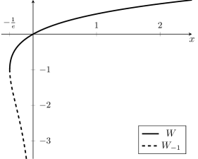
Figure 1. The functions $W(x)$ (solid line) and $W_{-1}(x)$ (dashed line)

For the upper branch, we will use that as $x\to\infty$ we have

$$W(x)=\log x-\log\log x+o(1),$$

and note that $W(x)e^{W(x)}=x$ implies $e^{W(x)}=x/W(x)$ if $x\neq 0$. This latter property clearly holds for any branch of $W$.

We encounter the lower branch as a solution to the equation $x\log(1/x)=1/(ey)$. A little rearranging gives $(\log x)e^{\log x}=-1/(ey)$, and hence $\log x$ is given by some branch of the Lambert $W$-function applied to $-1/(ey)$. If we know that $x\in\interval[oo]{0}{1/e}$ and $y\geq 1$ then the solution is

$$x=e^{W_{-1}(-1/(ey))}=\frac{1}{ey}\cdot\frac{1}{-W_{-1}(-1/(ey))}.$$

For brevity we introduce $K\colon\interval[co]{1}{\infty}\to\interval[co]{1}{\infty}$ for the function $K(y)=-W_{-1}(-1/(ey))$ appearing above. Then for $x\in\interval[oo]{0}{1/e}$ and $y\geq 1$ we have

$$x\log\frac{1}{x}=\frac{1}{ey}\quad\Longrightarrow\quad x=\frac{1}{eyK(y)}.$$

Standard properties of $W_{-1}$ give that $K$ is continuous, increasing, and as $x\to\infty$ satisfies $K(x)\sim\log x$, see [17].

For yet another equation we only need an asymptotic solution, but up to an additive $o(1)$ error term. Suppose that $x$ and $y$ are positive reals such that

$$y=\frac{e^{x}}{\log x}.$$

Then as $y\to\infty$ we have

(19) $$x =\log y+\log\log\log y+o(1).$$

To see this, substitute $x=\log y+\log\log\log y+z$ to obtain

$$e^{z}\log\log y=\log(\log y+\log\log\log y+z).$$

If $z=0$ the left-hand side is too small, but for constant $z$ and large enough $y$ the left-hand side is too large, so $z>0$ and $z=o(1)$.

Similarly, if $x$ and $y$ are positive reals such that

$$y=\frac{xe^{x}}{\log x},$$

then as $y\to\infty$ we have

$$x=\log y-\log\log y+\log\log\log y+o(1).$$

4.2. The hard-core model and entropy

In this subsection, we develop a refinement of an entropy argument of Shearer [52]. See e.g. the book by Alon and Spencer [8] for an introduction to the necessary entropy material. Some minor changes to Shearer’s proof are necessary to handle a general positive fugacity $\lambda$, but the case $\lambda=1$ of the proof below simply corresponds to a rather precise description of Shearer’s original method. The result is most useful when one has control of the term $K\big{(}y\lambda/\log Z_{F}(\lambda)\big{)}$. It boils down to bounding the number of independent sets in $F$ in terms of the size of $F$, and in later relevant sections we establish such results in context.

Lemma 19.

For any graph $F$ on $y$ vertices and any positive real $\lambda$,

$$\frac{\lambda Z_{F}^{\prime}(\lambda)}{Z_{F}(\lambda)}\geq\frac{\log Z_{F}(\lambda)}{K\big{(}y\lambda/\log Z_{F}(\lambda)\big{)}}.$$

Proof.

In the proof we write $Z$ instead of $Z_{F}(\lambda)$ for brevity and write $\log_{2}$ for the base-2 logarithm. For $x\in(0,1)$, let

$$h(x)=-x\log_{2}x-(1-x)\log_{2}(1-x)$$

be the binary entropy function (also satisfying $h(0)=h(1)=0$). For the hard-core model on $F$ at fugacity $\lambda$, we write $\mathbf{I}$ for a random independent set and $\phi=\mathbb{E}|\mathbf{I}|/y$ for the occupancy fraction. We desire a lower bound on $\mathbb{E}|\mathbf{I}|$. We first prove that

(20) $$\log Z\leq y\phi\log(e\lambda/\phi).$$

To this end, we compute the entropy $H(\mathbf{I})$,

$$H(\mathbf{I}) =-\sum_{I\in\mathcal{I}(F)}\frac{\lambda^{|I|}}{Z}\log_{2}\frac{\lambda^{|I|}}{Z}=\log_{2}Z-\sum_{I\in\mathcal{I}(F)}|I|\frac{\lambda^{|I|}}{Z}\log_{2}\lambda$$

$$=\log_{2}Z-\mathbb{E}|\mathbf{I}|\log_{2}\lambda,$$

so that by the subadditivity of the entropy and the concavity of $h$ we have

$$\log_{2}Z =\mathbb{E}|\mathbf{I}|\log_{2}\lambda+H(\mathbf{I})$$

$$\leq\mathbb{E}|\mathbf{I}|\log_{2}\lambda+\sum_{u\in V(F)}H(\mathbf{1}_{u\in\mathbf{I}})$$

$$=y\phi\log_{2}\lambda+\sum_{u\in V(F)}h\big{(}\mathbb{P}(u\in\mathbf{I})\big{)}\leq y\big{(}\phi\log_{2}\lambda+h(\phi)\big{)}.$$

Inequality (20) follows since for all $x\in\interval[oc]{0}{1}$ we have $h(x)\leq x\log_{2}(e/x)$, and $h(0)=0=\lim_{x\to 0}x\log_{2}(e/x)$. Note that we only use logarithms to base $2$ in the above calculations, and work with the natural logarithm elsewhere, including in (20).

The right-hand side of (20) is an increasing function of $\phi$ because the partial derivative with respect to $\phi$ is $y\log(\lambda/\phi)$ and in the hard-core model

$$\phi=\frac{1}{y}\sum_{u\in V(F)}\mathbb{P}(u\in\mathbf{I})\leq\frac{1}{y}\sum_{u\in V(F)}\mathbb{P}(u\in\mathbf{I}\mid N(u)\cap\mathbf{I}=\varnothing)=\frac{\lambda}{1+\lambda}<\lambda.$$

Hence we bound $\phi$ from below by solving (20) with equality, leading to

$$\frac{\phi}{e\lambda}\log\frac{e\lambda}{\phi}=\frac{\log Z}{ey\lambda}.$$

The right-hand side lies in $[0,1/e]$ since $Z\leq{(1+\lambda)}^{y}$. The exact solution is naturally expressed in terms of the function $K$ (see Subsection 4.1), giving

$$\mathbb{E}|\mathbf{I}|=y\phi\geq\frac{\log Z_{F}(\lambda)}{K\big{(}y\lambda/\log Z_{F}(\lambda)\big{)}}.\qed$$

4.3. The hard-core model with bounded average degree

The following lemma has essentially already appeared [19].

Lemma 20.

For any graph $F$ on $y$ vertices with average degree $d$ and any positive real $\lambda$,

(21) $$\frac{\lambda Z_{F}^{\prime}(\lambda)}{Z_{F}(\lambda)} \geq\frac{\lambda}{1+\lambda}y{(1+\lambda)}^{-d},\quad\text{and}$$

(22) $$\log Z_{F}(\lambda) \geq\begin{cases}y\log(1+\lambda)&\text{ if $d=0$,}\\ \frac{y}{d}\left(1-{(1+\lambda)}^{-d}\right)&\text{ if $d>0$.}\end{cases}$$

Proof.

We apply the analysis from Subsection 3.2 to $F$. Let $\mathbf{I}$ be a random independent set from the hard-core model at fugacity $\lambda$ on $F$. First, we have for any $u\in V(F)$,

$$\mathbb{P}(u\in\mathbf{I})=\frac{\lambda}{1+\lambda}\mathbb{P}(\mathbf{I}\cap N(u)=\varnothing)\geq\frac{\lambda}{1+\lambda}{(1+\lambda)}^{-\deg(u)},$$

because the spatial Markov property gives that $\mathbf{I}\cap N(v)$ is a random independent set drawn from the hard-core model on the subgraph $\mathbf{F}_{N(v)}$ of $F[N(v)]$ induced by the externally uncovered neighbours of $u$. The final inequality comes from the fact that any realisation of $\mathbf{F}_{N(v)}$ has $Z_{\mathbf{F}_{N(v)}}(\lambda)\leq{(1+\lambda)}^{\deg(u)}$. The lemma follows by convexity:

(23) $$\mathbb{E}|\mathbf{I}|=\sum_{u\in V(F)}\mathbb{P}(u\in\mathbf{I}) \geq\frac{\lambda}{1+\lambda}\sum_{u\in V(F)}{(1+\lambda)}^{-\deg(u)}$$

(24) $$\geq\frac{\lambda}{1+\lambda}y{(1+\lambda)}^{-d},$$

and integrating this bound gives the required lower bound on $\log Z_{F}(\lambda)$. ∎

Note that the above lower bound on $\log Z_{F}(\lambda)$ smoothly weakens as $d$ increases from zero, in that the expression for $d=0$ is simply the limit when $d$ tends to $0$ of the expression for positive $d$ (in fact with equality instead of inequality).

5. Bounded local maximum average degree

In this section we prove generalisations of Theorems 4–6. The key idea is to weaken the condition of triangle-freeness to having bounded average degree in any subgraph of a neighbourhood.

5.1. Local occupancy with bounded local mad

We begin with the relevant local occupancy result.

Lemma 21.

Let ${(a_{u})}_{u}$ be a sequence of nonnegative real numbers indexed by the vertices of a graph $G$ such that $\operatorname{mad}(G[N(u)])\leq a_{u}$ for each $u\in V(G)$. Then the following statements hold for any $\lambda>0$.

1. For any collection ${(d_{u})}_{u\in V(G)}$ of positive reals, a choice of parameters that minimises $\beta_{u}+\gamma_{u}d_{u}$ for all $u\in V(G)$ subject to strong local ${(\beta_{u},\gamma_{u})}_{u}$-occupancy in the hard-core model on $G$ at fugacity $\lambda$ is

   $$\gamma_{u} \coloneqq\frac{1+\lambda}{\lambda}\frac{{(1+\lambda)}^{a_{u}}\log(1+\lambda)}{1+W(d_{u}{(1+\lambda)}^{a_{u}}\log(1+\lambda))}$$

   $$\beta_{u} \coloneqq\frac{\gamma_{u}{(1+\lambda)}^{\frac{{(1+\lambda)}^{1+a_{u}}}{\gamma_{u}\lambda}-a_{u}}}{e\log(1+\lambda)},$$

   and under this choice, for all $u\in V(G)$,

   $$\beta_{u}+\gamma_{u}d_{u}=\frac{1+\lambda}{\lambda}\frac{d_{u}{(1+\lambda)}^{a_{u}}\log(1+\lambda)}{W(d_{u}{(1+\lambda)}^{a_{u}}\log(1+\lambda))}.$$

2. For any $u\in V(G)$ and any subgraph $F$ of $G[N(u)]$ on $y$ vertices,

   $$\log Z_{F}(\lambda)\geq\begin{cases}y\log(1+\lambda)&\text{ if $a_{u}=0$,}\\ \frac{y}{a_{u}}(1-{(1+\lambda)}^{-a_{u}})&\text{ if $a_{u}>0$.}\end{cases}$$

Proof.

Let $u$ be an arbitrary vertex of $G$, and suppose that $F\subseteq G[N(u)]$ has $y$ vertices. By assumption we know that $F$ has average degree at most $a_{u}$, and so Lemma 20 directly yields (ii). For (i) we note that $Z_{F}(\lambda)\leq{(1+\lambda)}^{y}$ and hence by Lemma 20 we have

$$\beta_{u}\frac{\lambda}{1+\lambda}\frac{1}{Z_{F}(\lambda)}+\gamma_{u}\frac{\lambda Z^{\prime}_{F}(\lambda)}{Z_{F}(\lambda)}\geq\frac{\lambda}{1+\lambda}\Big{(}\beta_{u}{(1+\lambda)}^{-y}+\gamma_{u}y{(1+\lambda)}^{-a_{u}}\Big{)},$$

and we define the right-hand side to be $g(y)$.

The function $g$ is strictly convex with a stationary minimum at

$$y^{*}=a_{u}+\frac{\log\left(\frac{\beta_{u}}{\gamma_{u}}\log(1+\lambda)\right)}{\log(1+\lambda)},$$

and if we set $g(y^{*})=1$ for strong local $(\beta_{u},\gamma_{u})$-occupancy, and solve for $\beta_{u}$ we obtain the definition given in the statement of the lemma. Then the function $\beta_{u}+\gamma_{u}d_{u}$ is strictly convex in $\gamma_{u}$, and the given $\gamma_{u}$ is the unique minimiser. One checks that, indeed, setting $\beta_{u}$ and $\gamma_{u}$ to the announced values, and writing $D_{u}$ for $d_{u}{(1+\lambda)}^{a_{u}}\log(1+\lambda)$, we have

$$\beta_{u}=\frac{1+\lambda}{\lambda}\cdot\frac{D_{u}}{W(D_{u})\cdot(1+W(D_{u}))},$$

and hence

$$\beta_{u}+\gamma_{u}d_{u}=\frac{1+\lambda}{\lambda}\left(\frac{D_{u}}{W(D_{u})(1+W(D_{u}))}+\frac{D_{u}}{1+W(D_{u})}\right)=\frac{1+\lambda}{\lambda}\frac{D_{u}}{W(D_{u})}$$

as announced. Furthermore,

$$y^{*}=\frac{W(D_{u})}{\log(1+\lambda)},$$

and hence indeed

$$g(y^{*}) =\frac{D_{u}\cdot{(1+\lambda)}^{-W(D_{u})/\log(1+\lambda)}}{W(D_{u})(1+W(D_{u}))}+\frac{W(D_{u})}{1+W(D_{u})}$$

$$=\frac{1}{1+W(D_{u})}+\frac{W(D_{u})}{1+W(D_{u})}=1.\qed$$

Note the parameters (3) obtained before in [18] for triangle-free graphs arise in the special case of the above lemma when $a_{u}=0$ and $d_{u}=\Delta$ for all $u$.

5.2. An excluded cycle length

If a graph contains no subgraph isomorphic to the cycle $C_{k}$, then the local path length in $G$ is bounded. It follows from a theorem of Erdős and Gallai [27] that we may use Lemma 21 with $a_{u}=k-3$ in particular, and then apply the main framework to prove the following result.

Theorem 22.

For any graph $G$ of maximum degree $\Delta$ that contains no subgraph isomorphic to $C_{k}$, for some $k\in\{3,\dotsc,\Delta+1\}$, the following statements hold.

1. For any $\lambda>0$, the occupancy fraction of the hard-core model on $G$ at fugacity $\lambda$ satisfies

   $$\frac{1}{|V(G)|}\frac{\lambda Z_{G}^{\prime}(\lambda)}{Z_{G}(\lambda)}\geq\max_{0\leq x\leq\lambda}\left\{\frac{x}{1+x}\frac{W(\Delta{(1+x)}^{k-3}\log(1+x))}{\Delta{(1+x)}^{k-3}\log(1+x)}\right\}.$$

2. For any $\varepsilon>0$ there exists $\delta_{0}$ such that there is a fractional colouring of $G$ where each $u\in V(G)$ is coloured with a subset of the interval

   $$\interval[co,scaled]{0}{(1+\varepsilon)\max\left\{\frac{\deg(u)}{\log(\deg(u)/k)},\,\frac{\delta_{0}}{\log\delta_{0}}k\right\}}.$$

   In particular, the fractional chromatic number of $G$ satisfies $\chi_{f}(G)\leq(1+o(1))\Delta/\log(\Delta/k)$ as $\Delta\to\infty$.

3. For any $\varepsilon>0$ there exist $\delta_{0}$ and $\Delta_{0}$ such that the following holds for all $\Delta\geq\Delta_{0}$. If $\mathscr{H}=(L,H)$ is a cover of $G$ such that for each $u\in V(G)$

   $$|L(u)|\geq(1+\varepsilon)\max\left\{\frac{\deg(u)}{\log(\deg(u)/(k\log\Delta))},\,\frac{\delta_{0}}{\log\delta_{0}}k\log\Delta\right\},$$

   then $G$ is $\mathscr{H}$-colourable. In particular, if $k=\Delta^{o(1)}$, then the correspondence chromatic number of $G$ satisfies $\chi_{c}(G)\leq(1+o(1))\Delta/\log\Delta$ as $\Delta\to\infty$.

Proof.

For every vertex $u\in V(G)$, no subgraph $F$ of $G[N(u)]$ contains a $(k-1)$-vertex path. Hence a theorem of Erdős and Gallai [27] implies that $F$ has average degree at most $k-3$. Having at our disposal the analysis of the hard-core model in graphs with bounded local $\operatorname{mad}$ given by Lemma 21 with $a_{u}=k-3$ for all $u$, the theorem follows easily from the main framework.

Setting $d_{u}=\Delta$ for all $u$, statement (i) then follows from Theorem 10 and the fact that the occupancy fraction of the hard-core model at fugacity $\lambda$ is strictly increasing in $\lambda$ [21, Prop. 1].

Statement (ii) follows from Theorem 11 and some asymptotic analysis. With $d_{u}=\deg(u)$ in Lemma 21 we deduce that $G$ admits a fractional colouring where each vertex $u$ is coloured by a subset of the interval $\interval[co]{0}{c_{u}}$ with

(25) $$c_{u} \coloneqq\beta_{u}+\gamma_{u}\deg(u)$$

(26) $$=\frac{1+\lambda}{\lambda}\frac{\deg(u){(1+\lambda)}^{k-3}\log(1+\lambda)}{W(\deg(u){(1+\lambda)}^{k-3}\log(1+\lambda))}.$$

Take $1/\lambda=k\log\delta_{0}$. This gives $\lambda=o(1)$ and $k\lambda=o(1)$ as $\delta_{0}\to\infty$ since $k\geq 3$. It follows from the asymptotic properties of $W$ (see Section 4.1) that, if $\deg(u)\geq\delta_{0}k$, then $c_{u}\sim\deg(u)/\log(\deg(u)/k)$ as $\delta_{0}\to\infty$.

For (iii) we apply Theorem 12. To fulfil (10), it suffices by Lemma 21(ii) to have

(27) $$\ell\geq\begin{cases}\frac{8\log(8\Delta^{4})}{\log(1+\lambda)}&\text{ if $k=3$,}\\ \frac{8(k-3)\log(8\Delta^{4})}{1-{(1+\lambda)}^{3-k}}&\text{ if $k>3$.}\end{cases}$$

because we then have $Z_{F}(\lambda)\geq 8\Delta^{4}$ for any $u\in V(G)$ and any subgraph $F$ of $G[N(u)]$ on $y\geq\ell/8$ vertices. We set

$$\ell=\begin{cases}\frac{8\log(8\Delta^{4})}{\log(1+\lambda)}&\text{ if $k=3$,}\\ \frac{8\log(8\Delta^{4})}{\frac{\lambda}{1+\lambda}-\frac{k-4}{2}{(\frac{\lambda}{1+\lambda})}^{2}}&\text{ if $k>3$.}\end{cases}$$

Supposing $\lambda=o(1)$ and $k\lambda=o(1)$ as $\Delta\to\infty$, we deduce that (27) holds provided $\Delta$ is large enough (by the expansion of ${(1+\lambda)}^{3-k}={(1-\frac{\lambda}{1+\lambda})}^{k-3}$), that $\ell=\omega(\log\Delta)$ and hence $\ell>7\log\Delta$ for all large enough $\Delta$, and that

$$\frac{\lambda}{1+\lambda}\frac{\ell}{1-\sqrt{(7\log\Delta)/\ell}}\sim 32\log\Delta.$$

To this end, we choose $1/\lambda=k\log\log\Delta$. Now we apply Lemma 21(i) with

$$d_{u}\coloneqq\frac{\max\{\deg(u),\delta_{0}\log\Delta\}}{\frac{\lambda}{1+\lambda}\frac{\ell}{1-\sqrt{(7\log\Delta)/\ell}}}.$$

Let $\beta_{u}$ and $\gamma_{u}$ be as given by the lemma in this case. It suffices to suppose that $\deg(u)\geq\delta_{0}k\log\Delta$ and, writing $\eta$ for $\sqrt{(7\log\Delta)/\ell}$ to improve readability, show that

(28) $$\frac{\lambda}{1+\lambda}\frac{\ell}{1-\eta}(\beta_{u}+\gamma_{u}d_{u}) =\frac{1+\lambda}{\lambda}\frac{\deg(u){(1+\lambda)}^{k-3}\log(1+\lambda)}{W\left(\frac{\deg(u)}{\frac{\lambda}{1+\lambda}\frac{\ell}{1-\eta}}{(1+\lambda)}^{k-3}\log(1+\lambda)\right)}$$

(29) $$\leq(1+\varepsilon)\frac{\deg(u)}{\log(\deg(u)/(k\log\Delta))},$$

which will hold if $\delta_{0}$ and $\Delta_{0}$ are large enough: this follows by the choice of $\ell$ and $\lambda$ and the asymptotic properties of $W$. ∎

5.3. Bounded local triangle count

The following result, where we suppose that each vertex of $G$ is contained in at most $t$ triangles, implies and elaborates upon Theorem 5. With $t=\Delta^{2}/f$ we regain the form of Theorem 5.

Theorem 23.

For any graph $G$ of maximum degree $\Delta$ in which each vertex is contained in at most $t\geq 1/2$ triangles, the following statements hold.

1. For any $\lambda>0$, the occupancy fraction of the hard-core model on $G$ at fugacity $\lambda$ satisfies

   $$\frac{1}{|V(G)|}\frac{\lambda Z_{G}^{\prime}(\lambda)}{Z_{G}(\lambda)}\geq\max_{0\leq x\leq\lambda}\left\{\frac{x}{1+x}\frac{W(\Delta{(1+x)}^{\sqrt{2t}}\log(1+x))}{\Delta{(1+x)}^{\sqrt{2t}}\log(1+x)}\right\}.$$

2. For any $\varepsilon>0$ there exists $\delta_{0}$ such that there is a fractional colouring of $G$ such that each $u\in V(G)$ is coloured with a subset of the interval

   $$\interval[co,scaled]{0}{(1+\varepsilon)\max\left\{\frac{\deg(u)}{\log(\deg(u)/\sqrt{t})},\,\frac{\delta_{0}}{\log\delta_{0}}\sqrt{t}\right\}}.$$

   In particular, the fractional chromatic number of $G$ satisfies $\chi_{f}(G)\leq(1+o(1))\Delta/\log(\Delta/\sqrt{t})$ as $\Delta\to\infty$.

3. For any $\varepsilon>0$ there exist $\delta_{0}$ and $\Delta_{0}$ such that the following holds for all $\Delta\geq\Delta_{0}$. If $\mathscr{H}=(L,H)$ is a cover of $G$ such that for each $u\in V(G)$

   $$|L(u)|\geq(1+\varepsilon)\max\left\{\frac{\deg(u)}{\log(\deg(u)/(\sqrt{t}\log\Delta))},\,\frac{\delta_{0}}{\log\delta_{0}}\sqrt{t}\log\Delta\right\},$$

   then $G$ is $\mathscr{H}$-colourable. In particular, if $t=\Delta^{o(1)}$, then the correspondence chromatic number of $G$ satisfies $\chi_{c}(G)\leq(1+o(1))\Delta/\log\Delta$ as $\Delta\to\infty$.

The requirement that $t$ be at least $1/2$ is not restrictive: for any $t\in\interval[co]{0}{1}$ each vertex being contained in at most $t$ triangles is equivalent to being triangle-free. This merely helps us avoid issues with small $t$ when choosing parameters. Before proving Theorem 23, we compare it with related earlier results. For convenience we restate a non-local Theorem 23(iii) with $t=\Delta^{2}/f$.

Corollary 24.

For any $\varepsilon>0$ there exists $\Delta_{0}$ such that the following holds for all $\Delta\geq\Delta_{0}$. For any graph $G$ of maximum degree $\Delta$ in which each vertex is contained in at most $\Delta^{2}/f$ triangles, where ${(\log\Delta)}^{2/\varepsilon}\leq f\leq\Delta^{2}+1$, we have $\chi_{c}(G)\leq(1+\varepsilon)\Delta/\log\sqrt{f}$.

Sketch proof.

Without loss of generality we may assume that $\varepsilon$ is smaller than an absolute constant. With $t=\Delta^{2}/f$ we have $\Delta/\sqrt{t}=\sqrt{f}$ and we need $f$ large enough in terms of $\Delta$ so that the asymptotic expansion of $W((1-o(1))\sqrt{f}/\log\Delta)=(1-o(1))\log\sqrt{f}$ is accurate enough. This occurs if e.g. $f\geq{(\log\Delta)}^{2/\varepsilon}$ when $\Delta$ is large enough in terms of $\varepsilon$. ∎

Improving on earlier results of Alon, Krivelevich and Sudakov [7] and Vu [54], a statement similar to Corollary 24 was recently proved by Achlioptas, Iliopoulos and Sinclair [1, Thm. II.5] for the list chromatic number. They however required a much stronger lower bound on $f$ of the form $f\geq\Delta^{\frac{2+2\varepsilon}{1+2\varepsilon}}{(\log\Delta)}^{2}$, this last expression being roughly $\Delta^{2-\varepsilon}$. They used this weaker statement together with a known reduction [7] from the ‘small $f$’ case to the easier ‘large $f$’ case to obtain a quantitatively weaker bound than in Theorem 5 for chromatic number. Armed with our stronger Corollary 24, we can perform this same reduction but without a noticeable degradation of the leading constant to obtain Theorem 5. After next showing Theorem 23, we give the reduction in Subsection 5.4. A large part of the proof of Theorem 23 is omitted, being nearly identical to the corresponding part in the proof of Theorem 22.

Sketch proof of Theorem 23.

Fix a vertex $u\in V(G)$ and any subgraph $F\subseteq G[N(v)]$ on $y$ vertices. By assumption, $F$ contains at most $t$ edges. It follows that the average degree of $F$ is at most

$$\min\left\{y-1,\frac{2t}{y}\right\}\leq\sqrt{2t}.$$

Indeed, the first bound is straightforward as there are at most $y-1$ possible neighbours for any vertex in $F$. The second is also straightforward from the handshaking lemma. The minimum is maximised at $t=\binom{y}{2}$, which yields the statement. Thus the theorem follows easily from the main framework by Lemma 21 with $a_{u}=\sqrt{2t}$ for all $u$. The remainder of the proof is nearly identical to the proof of Theorem 22 but with $\sqrt{2t}$ in the place of $k-3$, and it is omitted. ∎

5.4. Proof of Theorem 5

Due to the condition on $f$, Corollary 24 does not directly imply Theorem 5, at least not via (7). Instead we appeal to an iterative splitting procedure that was used similarly before [7, 1]. We include the details of the derivation for completeness. This requires two results which are shown with the help of the Lovász local lemma.

Lemma 25 ([7]).

For any graph $G$ of maximum degree $\Delta\geq 2$ in which the neighbourhood of every vertex spans at most $s$ edges, there exists a partition $V(G)=V_{1}\cup V_{2}$ such that $V_{i}$ for $i\in\{1,2\}$ induces a subgraph of maximum degree at most $\Delta/2+2\sqrt{\Delta\log\Delta}$ in which the neighbourhood of every vertex spans at most $s/4+2\Delta^{3/2}\sqrt{\log\Delta}$ edges.

Lemma 26 ([1], cf. also [7]).

Given $\Delta$ and $f$ sufficiently large, define the sequences ${(\Delta_{t})}_{t\geq 0}$ and ${(s_{t})}_{t\geq 0}$ as follows: $\Delta_{0}=\Delta$, $s_{0}=\Delta^{2}/f$, and

(30) $$\Delta_{t+1} =\Delta_{t}/2+2\sqrt{\Delta_{t}\log\Delta_{t}}, s_{t+1} =s_{t}/4+2\Delta_{t}^{3/2}\sqrt{\log\Delta_{t}}.$$

For any $\delta\in\interval[oo]{0}{1/100}$ and $\zeta>0$ such that $\zeta(2+\delta)<1/10$, let $j$ be the smallest nonnegative integer for which $f>{\left((1+\delta)\Delta/2^{j}\right)}^{\zeta(2+\delta)}$. Then $\Delta_{j}\leq(1+\delta)\Delta/2^{j}$ and $s_{j}\leq{\left((1+\delta)\Delta/2^{j}\right)}^{2}/f$.

Proof of Theorem 5.

Let $\varepsilon>0$. It suffices to prove that $\chi(G)\leq(1+\varepsilon)\Delta/\log\sqrt{f}$ for $f$ (and thus $\Delta$) sufficiently large. We may assume that $f\leq\Delta^{\varepsilon^{2}(2+\varepsilon^{2})}$, otherwise we can apply Corollary 24. Without loss of generality, we may also assume that $\varepsilon\leq 1/11$. Let $\delta=\zeta=\varepsilon^{2}$ (which is indeed less than $1/100$) so that $\zeta(2+\delta)<1/10$ and we may apply Lemma 26. Let $j=j(\Delta,f,\delta,\zeta)$ be the integer given therein and, starting with the trivial partition $\{V(G)\}$, iterate the following procedure $j$ times to form a partition of $V(G)$.

In one iteration of the procedure, for each part $W$ of the current partition, do the following. If the induced subgraph $G[W]$ has maximum degree at most $1$ then do nothing, or else split $W$ into two parts as given by Lemma 25.

The ultimate partition of $V(G)$ yields at most $2^{j}$ induced subgraphs of $G$, and by Lemma 26 each such subgraph $H$ has maximum degree at most $1$, or it has maximum degree at most $\Delta_{*}\coloneqq(1+\delta)\Delta/2^{j}$ and the property that every neighbourhood of $H$ spans at most $\Delta_{*}^{2}/f$ edges. Observe that $\Delta_{*}^{\zeta(2+\delta)}<f\leq{(2\Delta_{*})}^{\zeta(2+\delta)}$ due to the choice of $j$ in Lemma 26 and the fact that $f\leq\Delta^{\varepsilon^{2}(2+\varepsilon^{2})}\leq{((1+\delta)\Delta/2^{0})}^{\zeta(2+\delta)}$ —which implies that $j\geq 1$. Now either $\chi(H)\leq 2$ by (1), or $\chi(H)\leq(1+\zeta)\Delta_{*}/\log\sqrt{f}$ by Corollary 24 (for $f$, hence $\Delta_{*}$, sufficiently large). Therefore

$$\chi(G)\leq 2^{j}\max\left\{2,\,(1+\zeta)\frac{\Delta_{*}}{\log\sqrt{f}}\right\}=\max\left\{2^{j+1},\,(1+\zeta)\frac{(1+\delta)\Delta}{\log\sqrt{f}}\right\}.$$

We also have

$$\frac{(1+\delta)\Delta}{\Delta/(4\log\sqrt{f})}=2(1+\delta)\log f<f^{\frac{1}{\zeta(2+\delta)}}\leq 2\Delta_{*}=\frac{(1+\delta)\Delta}{2^{j-1}},$$

where the first inequality follows from a choice of large enough $f$ and the second holds by the above range for $f$ in terms of $\Delta_{*}$. This bounds the first argument in the maximisation as it yields that $2^{j+1}\leq\Delta/\log\sqrt{f}$. For the second argument, note that $(1+\zeta)(1+\delta)={(1+\varepsilon^{2})}^{2}\leq(1+\varepsilon)$ since $\varepsilon\leq 1/11$. ∎

5.5. Bounded local cycle count

In Subsections 5.2 and 5.3, we showed that our analysis of the hard-core model under bounded local $\operatorname{mad}$ can be applied effectively to graph with no $C_{k}$ and graphs for which each vertex is contained in few triangles. We next note how to combine these two ideas, hinting at some further flexibility in our approach.

Theorem 27.

For any graph $G$ of maximum degree $\Delta$ in which the subgraph induced by each neighbourhood contains at most $t$ copies of $P_{k-1}$, where $t\geq 1/2$ and $k\geq 3$, the following statements hold.

1. For any $\lambda>0$, the occupancy fraction of the hard-core model on $G$ at fugacity $\lambda$ satisfies

   $$\frac{1}{|V(G)|}\frac{\lambda Z_{G}^{\prime}(\lambda)}{Z_{G}(\lambda)}\geq\max_{0\leq x\leq\lambda}\left\{\frac{x}{1+x}\frac{W(\Delta{(1+x)}^{k-3+\sqrt{2t}}\log(1+x))}{\Delta{(1+x)}^{k-3+\sqrt{2t}}\log(1+x)}\right\}.$$

2. For any $\varepsilon>0$ there exists $\delta_{0}$ such that there is a fractional colouring of $G$ such that each $u\in V(G)$ is coloured with a subset of the interval

   $$\interval[co,scaled]{0}{(1+\varepsilon)\max\left\{\frac{\deg(u)}{\log(\deg(u)/(k+\sqrt{t}))},\,\frac{\delta_{0}}{\log\delta_{0}}(k+\sqrt{t})\right\}}.$$

   In particular, the fractional chromatic number of $G$ satisfies $\chi_{f}(G)\leq(1+o(1))\Delta/\log(\Delta/(k+\sqrt{t}))$ as $\Delta\to\infty$.

3. For any $\varepsilon>0$ there exist $\delta_{0}$ and $\Delta_{0}$ such that the following holds for all $\Delta\geq\Delta_{0}$. If $\mathscr{H}=(L,H)$ is a cover of $G$ such that for each $u\in V(G)$

   $$|L(u)|\geq(1+\varepsilon)\max\Bigg{\{} \frac{\deg(u)}{\log(\deg(u)/((k+\sqrt{t})\log\Delta))},\,$$

   $$\frac{\delta_{0}}{\log\delta_{0}}(k+\sqrt{t})\log\Delta\Bigg{\}},$$

   then $G$ is $\mathscr{H}$-colourable. In particular, if $k+\sqrt{t}=\Delta^{o(1)}$, then the correspondence chromatic number of $G$ satisfies $\chi_{c}(G)\leq(1+o(1))\Delta/\log\Delta$ as $\Delta\to\infty$.

Proof sketch.

Fix a vertex $u\in V(G)$ and any subgraph $F\subseteq G[N(u)]$ on $y$ vertices. By assumption, $F$ contains at most $t$ copies of $P_{k-1}$. It follows that the average degree of $F$ is at most

$$\min\left\{y-1,\,k-3+\frac{2t}{y}\right\}\leq k-3+\sqrt{2t}.$$

Indeed, the first bound is straightforward as there are at most $y-1$ possible neighbours for any vertex in $f$. For the second, we only need to remove at most $t$ edges from $F$ to destroy all copies of $P_{k-1}$, so that by the result of Erdős and Gallai [27] the remaining graph has at most $y(k-3)/2$ edges. Thus $F$ has at most $y(k-3)/2+t$ edges, implying the second bound. We consider the subcases $y\leq\sqrt{2t}$ and $y>\sqrt{2t}$ to crudely upper bound the minimum, from which the statement follows. Thus the theorem follows easily from the main framework by using Lemma 21 with $a_{u}=k-3+\sqrt{2t}$ for all $u$. Indeed the remainder of the proof is nearly identical to the proof of Theorem 22 but with $k-3+\sqrt{2t}$ in the place of $k-3$. The details are left to the interested reader. ∎

5.6. Neighbourhoods with an excluded bipartite subgraph

We remark that by other classic extremal results conclusions akin to those in Theorem 22 hold for a graph containing no subgraph of the form $K_{1}+T_{k-1}$, where $T_{k-1}$ denotes some arbitrary $(k-1)$-vertex tree. In fact, similar results hold (varying in the leading constants) for graphs containing no $K_{1}+H$ where $H$ is bipartite. Such observations were already made in [7], where one uses their analogue of Theorem 5 which has a larger, unspecified leading constant. Our framework permits the transfer of bounds on the extremal number of $H$ to chromatic number bounds in $(K_{1}+H)$-free graphs with better leading constants than via the reduction in [7]. For example, in another ‘smooth’ extension of Theorem 2 one can also show with our framework that for fixed $s\geq t\geq 1$ and $G$ with no $K_{1}+K_{s,t}$, we have the bound $\chi(G)\leq(t+o(1))\Delta/\log\Delta$ as $\Delta\to\infty$. Of course one can also show a suite of local, list, and correspondence strengthenings, and even a ‘few copies’ version along the lines of Theorem 27. We do not give the details as the method is essentially the same as the other proofs we present in this section. The main idea is to use an extremal number result to bound $\operatorname{mad}(G[N(u)])$ for all $u\in V(G)$ (in the case mentioned above we use the well-known result on the Zarankiewicz Problem of Kővári, Sós, and Turán [43]), and then make suitable choices of $\ell$ and $\lambda$. With the main work done by our framework and the details given already in this section, these remaining tasks are quite straightforward.

6. Bounded local Hall ratio

The following result generalises Theorem 7. Recall that the Hall ratio of a graph $G$ is $\rho(G)=\max\{|V(H)|/\alpha(H)\mid H\subseteq G\}$.

Theorem 28.

Let $K\colon\interval[co]{1}{\infty}\to\interval[co]{1}{\infty}$ be defined in terms of the lower branch of the Lambert-W function by $K(y)\coloneqq-W_{-1}(-1/(ey))$.

For any graph $G$ of maximum degree $\Delta$ in which the neighbourhood of every vertex $u\in V(G)$ induces a subgraph of Hall ratio at most $\rho_{u}\geq 1$, and with $\rho\coloneqq\max_{u\in V(G)}\rho_{u}$, the following statements hold.

1. For any $\lambda>0$, setting $k(x)=K(\rho x/\log(1+x))$, the occupancy fraction of the hard-core model on $G$ at fugacity $\lambda$ satisfies

   $$\frac{1}{|V(G)|}\frac{\lambda Z_{G}^{\prime}(\lambda)}{Z_{G}(\lambda)}\geq\max_{0\leq x\leq\lambda}\left\{\frac{W(k(x)\Delta x/(1+x))}{k(x)\Delta}\right\}.$$

2. For any $\varepsilon>0$ there exists $\delta_{0}$ such that there is a fractional colouring of $G$ such that each $u\in V(G)$ is coloured with a subset of the interval

   $$\interval[co,scaled]{0}{(1+\varepsilon)\max\left\{\frac{K(\rho_{u})\deg(u)}{\log(K(\rho_{u})\deg(u))},\,\frac{K(\rho_{u})\delta_{0}}{\log(K(\rho_{u})\delta_{0})}\right\}}.$$

3. For any $\varepsilon>0$ there exist $\delta_{0}$ and $\Delta_{0}$ such that the following holds for all $\Delta\geq\Delta_{0}$ and $\delta=\delta_{0}\rho\log\Delta$. If $\mathscr{H}=(L,H)$ is a cover of $G$ such that for each $u\in V(G)$

   $$|L(u)|\geq(1+\varepsilon)\max\left\{\frac{K(\rho_{u})\deg(u)}{\log\left(\frac{K(\rho_{u})\deg(u)}{\rho\log\Delta}\right)},\,\frac{K(\rho_{u})\delta}{\log\left(\frac{K(\rho_{u})\delta}{\rho\log\Delta}\right)}\right\},$$

   then $G$ is $\mathscr{H}$-colourable. In particular, the correspondence chromatic number of $G$ satisfies $\chi_{c}(G)\leq(1+o(1))K(\rho)\Delta/\log(K(\rho)\Delta/\rho)$ as $\Delta\to\infty$.

Note also that $K(\rho_{u})\sim\log\rho_{u}$ as $\rho_{u}\to\infty$.

6.1. Local occupancy with bounded local Hall ratio

We begin with the requisite local analysis of the hard-core model, which relies critically on Lemma 19.

Lemma 29.

For any graph $G$ in which the neighbourhood of every vertex $u\in V(G)$ induces a subgraph of Hall ratio at most $\rho_{u}\geq 1$, the following holds.

1. For any $\lambda>0$ and collection ${(d_{u})}_{u\in V(G)}$ of positive reals, a choice of parameters that minimises $\beta_{u}+\gamma_{u}d_{u}$ for all $u\in V(G)$ subject to strong local ${(\beta_{u},\gamma_{u})}_{u}$-occupancy in the hard-core model on $G$ at fugacity $\lambda$ is

   $$\beta_{u} =\frac{1+\lambda}{\lambda}\cdot\frac{\exp(W(k_{u}d_{u}\lambda/(1+\lambda)))}{1+W(k_{u}d_{u}\lambda/(1+\lambda))}\quad\text{and}$$

   $$\gamma_{u} =\frac{k_{u}}{1+W(k_{u}d_{u}\lambda/(1+\lambda))},$$

   where $k_{u}=K\big{(}\rho_{u}\lambda/\log(1+\lambda)\big{)}$. Moreover, with $k=\max_{u\in V(G)}k_{u}$ and $\beta$ and $\gamma$ obtained by replacing $k_{u}$ in the definitions of $\beta_{u}$ and $\gamma_{u}$ by $k$, the graph $G$ has strong local $(\beta,\gamma)$-occupancy.

2. For any $u\in V(G)$ and any subgraph $F$ of $G[N(u)]$ on $y$ vertices,

   $$\log Z_{F}(\lambda)\geq\frac{y}{\rho_{u}}\log(1+\lambda).$$

Proof.

Fix an arbitrary vertex $u\in V(G)$, and let $F$ be any subgraph of $G[N(u)]$ on $y$ vertices. Then since $G[N(u)]$ has Hall ratio at most $\rho_{u}$, the graph $F$ contains an independent set of size at least $y/\rho_{u}$. This immediately implies part (ii). We can now bound $\lambda Z^{\prime}_{F}(\lambda)/Z_{F}(\lambda)$ from below with Lemma 19:

$$\frac{\lambda Z_{F}^{\prime}(\lambda)}{Z_{F}(\lambda)}\geq\frac{\log Z_{F}(\lambda)}{K(y\lambda/\log Z_{F}(\lambda))}\geq\frac{\log Z_{F}(\lambda)}{K(\rho_{u}\lambda/\log(1+\lambda))}=\frac{\log Z_{F}(\lambda)}{k_{u}},$$

where the second inequality follows from applying part (ii) in the denominator.

For part (i), we start working with arbitrary positive reals $\beta_{u},\gamma_{u}$, and show that choosing them as in the statement gives the desired properties. We have

$$\beta_{u}\frac{\lambda}{1+\lambda}\frac{1}{Z_{F}(\lambda)}+\gamma_{u}\frac{\lambda Z_{F}^{\prime}(\lambda)}{Z_{F}(\lambda)}\geq\beta_{u}\frac{\lambda}{1+\lambda}e^{-\log Z_{F}(\lambda)}+\gamma_{u}\frac{\log Z_{F}(\lambda)}{k_{u}},$$

which we can minimise over all possible nonnegative values of $\log Z_{F}(\lambda)$. Let the function $g\colon\mathbb{R}\to\mathbb{R}$ be defined such that the right-hand side above is $g(\log Z_{F}(\lambda))$, and note that $k_{u}$ is independent of $F$. It is easy to verify that $g^{\prime\prime}(z)=\beta_{u}\frac{\lambda}{1+\lambda}e^{-z}>0$, and hence that $g$ is strictly convex. Then we bound $g(\log Z_{F}(\lambda))$ from below by finding the unique stationary point of $g(z)$, which must be a global minimum. This occurs at

$$z^{*}=\log\left(\frac{\beta_{u}}{\gamma_{u}}\frac{\lambda}{1+\lambda}k_{u}\right),$$

giving

$$g\big{(}\log Z_{F}(\lambda)\big{)}\geq g(z^{*})=\frac{\gamma_{u}}{k_{u}}\left(1+\log\left(\frac{\beta_{u}}{\gamma_{u}}\frac{\lambda}{1+\lambda}k_{u}\right)\right).$$

This is equal to $1$ when $\beta_{u}$ is given in terms of $\gamma_{u}$ by

(31) $$\beta_{u}=\frac{\gamma_{u}}{k_{u}}\frac{1+\lambda}{\lambda}e^{\frac{k_{u}}{\gamma_{u}}-1},$$

and taking $\gamma_{u}$ as in the statement of the lemma, that is,

$$\gamma_{u}=\frac{k_{u}}{1+W(k_{u}d_{u}\lambda/(1+\lambda))},$$

means $\beta_{u}$ as given by (31) agrees with $\beta_{u}$ as in the statement of the lemma. This completes the proof that $G$ has strong ${(\beta_{u},\gamma_{u})}_{u}$-local occupancy.

For local occupancy with uniform $(\beta,\gamma)$ parameters it suffices to observe that increasing $\beta_{u}$ and $\gamma_{u}$ retains local occupancy, and that $\beta_{u}$ and $\gamma_{u}$ are increasing functions of $k_{u}$, and hence of $\rho_{u}$. This is easy to do with a little calculus: first, because $K\colon\interval[co]{1}{\infty}\to\interval[co]{1}{\infty}$ is increasing, we deduce that $k_{u}$ increases with $\rho_{u}$. Second, considering $\gamma_{u}$ and writing $t=d_{u}\lambda/(1+\lambda)$ for convenience, observe that the function $x\to x/(1+W(xt))$ is increasing over $\interval[co]{1}{\infty}$, its derivative being $x\to\frac{{W(xt)}^{2}+W(tx)+1}{{(W(tx)+1)}^{3}}$, which is positive if $x\geq 1$ as $t>0$. Third, considering now $\beta_{u}$ and using the same notation, the function $x\to\frac{\exp(W(xt))}{1+W(xt)}$ is increasing over $\interval[co]{1}{\infty}$ its derivate being $x\to\frac{\exp(W(xt))\cdot{W(xt)}^{2}}{x\cdot{(W(xt)+1)}^{3}}$, which is positive if $x\geq 1$.

We note in addition that one can show the choice of $\gamma_{u}$ (with $\beta_{u}$ as in (31)) minimises $\beta_{u}+\gamma_{u}d_{u}$ with some calculus similar to the analysis of $g$. ∎

6.2. Proof of Theorem 28

Proof of Theorem 28.

We simply apply the main framework to derive the results. Lemma 29 gives for each collection ${(d_{u})}_{u\in V(G)}$ a choice for every $u\in V(G)$ of $\beta_{u}$ and $\gamma_{u}$ such that the hard-core model on $G$ at fugacity $\lambda$ has strong local ${(\beta_{u},\gamma_{u})}_{u}$-local occupancy, and we compute

$$\beta_{u}+\gamma_{u}d_{u}=\frac{k_{u}d_{u}}{W(k_{u}d_{u}\lambda/(1+\lambda))}.$$

We will choose $d_{u}$ carefully to obtain each part of the theorem.

For (i) we are interested in local occupancy with uniform parameters but Lemma 29 also gives suitable $\beta$ and $\gamma$ for this. Choosing $d_{u}=\Delta$, applying Theorem 10, and recalling that occupancy fraction is monotone increasing in $\lambda$ yields (i).

Statement (ii) follows from Theorem 11 and some asymptotic analysis. With the choice $d_{u}=\max\{\deg(u),\delta\}$ any $\lambda>0$ we have

$$\beta_{u}+\gamma_{u}\deg(u)\leq\frac{d_{u}k_{u}}{W(d_{u}k_{u}\lambda/(1+\lambda))},$$

with $\lambda=1/\log\delta$, for large enough $\delta$ in terms of $\varepsilon$ we have

$$\beta_{u}+\gamma_{u}\deg(u)\leq(1+\varepsilon)\frac{K(\rho_{u})d_{u}}{\log(K(\rho_{u})d_{u})},$$

as required for (ii). For the asymptotic properties of $K$ and $W$ necessary for the final step we refer to Subsection 4.1.

To obtain (iii) we aim to apply Theorem 12, and hence we must give a real $\ell>7\log\Delta$ and show that $\log Z_{F}(\lambda)$ is large enough for all subgraphs of $G$ induced by subsets of neighbourhoods of size at least $\ell/8$. By Lemma 29(ii), every graph $F$ induced by a subset of $N(u)$ with $y$ vertices satisfies

$$\log Z_{F}(\lambda)\geq\frac{y}{\rho_{u}}\log(1+\lambda).$$

As before, we may assume that $|L(u)|\leq\Delta$ for otherwise we can simply colour such a vertex $u$ at the end. So with $\ell=40\rho\log\Delta/\log(1+\lambda)$, if $y\geq\ell/8$ and $\Delta\geq 8$, then

$$\log Z_{F}(\lambda)\geq\frac{5\rho\log\Delta}{\rho_{u}}\geq\log(\Delta^{5})\geq\log(8\Delta^{4}),$$

as required for (10). Since $\rho\geq 1$, provided we choose $\lambda$ smaller than some absolute constant (e.g. $302$) we will have $\ell>7\log\Delta$. Then writing $\eta=\sqrt{(7\log\Delta)/\ell}$ we infer that $G$ is $\mathscr{H}$-colourable when

$$|L(u)|\geq\frac{\lambda}{1+\lambda}\frac{\ell}{1-\eta}\left(\beta_{u}+\gamma_{u}\frac{\deg(u)}{\frac{\lambda}{1+\lambda}\frac{\ell}{1-\eta}}\right).$$

This motivates the choice

$$d_{u}=\frac{\max\left\{\deg(u),\delta\right\}}{\frac{\lambda}{1+\lambda}\frac{\ell}{1-\eta}},$$

so that to apply Theorem 12 it now suffices that

$$|L(u)|\geq\max\left\{\frac{k_{u}\deg(u)}{W\left(\frac{k_{u}\deg(u)(1-\eta)\log(1+\lambda)}{40\rho\log\Delta}\right)},\,\frac{k_{u}\delta}{W\left(\frac{k_{u}\delta(1-\eta)\log(1+\lambda)}{40\rho\log\Delta}\right)}\right\}.$$

To give an asymptotic analysis of this bound we want to apply $W$ to a term that tends to infinity. With $\delta=\delta_{0}\rho\log\Delta$ we choose $\lambda$ such that $\log(1+\lambda)=1/\log\delta_{0}$ so that with $\delta_{0}$ large enough in terms of $\varepsilon$ we have not only $\ell>7\log\Delta$ but also $\eta$ small enough that the above lower bound on $|L(u)|$ is implied by

$$|L(u)|\geq(1+\varepsilon)\max\left\{\frac{K(\rho_{u})\deg(u)}{\log\left(\frac{K(\rho_{u})\deg(u)}{\rho\log\Delta}\right)},\,\frac{K(\rho_{u})\delta}{\log\left(\frac{K(\rho_{u})\delta}{\rho\log\Delta}\right)}\right\},$$

as required. ∎

7. Bounded clique number

The following result generalises Theorem 8.

Theorem 30.

For any graph $G$ of maximum degree $\Delta$ in which the largest clique containing any vertex $u\in V(G)$ has size at most $\omega_{u}\geq 3$, the following statements hold. We write $\omega=\max_{u\in V(G)}\{\omega_{u}\}$ for an upper bound on the clique number of $G$.

1. For any $\lambda>0$, the occupancy fraction of the hard-core model on $G$ at fugacity $\lambda$ satisfies as $\Delta\to\infty$,

   $$\frac{1}{|V(G)|}\frac{\lambda Z_{G}^{\prime}(\lambda)}{Z_{G}(\lambda)}\geq(1-o(1))\max\left\{\frac{\log\Delta}{(\omega-2)\Delta\log\log\Delta},\frac{1}{2\Delta}\sqrt{\frac{\log\Delta}{\log(\omega-1)}}\right\}.$$

2. For any $\varepsilon>0$ there exists $\delta_{0}$ such that there is a fractional colouring of $G$ such that each $u\in V(G)$ is coloured with a subset of the smaller of the following two intervals:

   (32) $$\interval[co,scaled]{0}{(1+\varepsilon)\max\left\{(\omega_{u}-2)\frac{\deg(u)\log\log\deg(u)}{\log\deg(u)},\,(\omega_{u}-2)\frac{\delta_{0}\log\log\delta_{0}}{\log\delta_{0}}\right\}},$$

   (33) $$\interval[co,scaled]{0}{(1+\varepsilon)\max\left\{2\deg(u)\sqrt{\frac{\log(\omega_{u}-1)}{\log\deg(u)}},\,2\delta_{0}\sqrt{\frac{\log(\omega_{u}-1)}{\log\delta_{0}}}\right\}}.$$

   In particular, the fractional chromatic number of $G$ satisfies

   $$\chi_{f}(G)\leq(1+o(1))\min\left\{(\omega-2)\frac{\Delta\log\log\Delta}{\log\Delta},\,2\Delta\sqrt{\frac{\log(\omega-1)}{\log\Delta}}\right\}$$

   as $\Delta\to\infty$.

3. For all $\varepsilon>0$ there exist $\delta_{0}$ and $\Delta_{0}$ such that the following holds for all $\Delta\geq\Delta_{0}$ and $\delta=\delta_{0}k$ where

   (34) $$k =\min\left\{{\left(e^{2}\log(8\Delta^{4})\right)}^{\omega-1},\,\exp\left(\sqrt{4\log(\omega-1)\cdot(1+\varepsilon)\log(8\Delta^{4})}\right)\right\}.$$

   If $\mathscr{H}=(L,H)$ is a cover of $G$ such that for each $u\in V(G)$, the size of $L(u)$ is at least the smaller of the two expressions below,

   (35) $$(1+\varepsilon)\max\left\{(\omega_{u}-2)\frac{\deg(u)\log\log(\deg(u)/k)}{\log(\deg(u)/k)},\,(\omega_{u}-2)\frac{\delta\log\log(\delta/k)}{\log(\delta/k)}\right\},$$

   (36) $$(1+\varepsilon)\max\left\{2\deg(u)\sqrt{\frac{\log(\omega_{u}-1)}{\log(\deg(u)/k)}},\,2\delta\sqrt{\frac{\log(\omega_{u}-1)}{\log(\delta/k)}}\right\},$$

   then $G$ is $\mathscr{H}$-colourable.

   In particular, the correspondence chromatic number of $G$ satisfies

   $$\chi_{c}(G)\leq(1+o(1))\min\left\{(\omega-2)\frac{\Delta\log\log\Delta}{\log\Delta},\,5\Delta\sqrt{\frac{\log(\omega-1)}{\log\Delta}}\right\}$$

   as $\Delta\to\infty$.

For convenience, we restate the independence number bound that either of parts (i) and (ii) above immediately yield.

Corollary 31.

For any graph $G$ of clique number $\omega$ and maximum degree $\Delta$, the independence number of $G$ satisfies as $\Delta\to\infty$

(37) $$\alpha(G)\geq(1-o(1))|V(G)|\max\left\{\frac{\log\Delta}{(\omega-2)\Delta\log\log\Delta},\frac{1}{2\Delta}\sqrt{\frac{\log\Delta}{\log(\omega-1)}}\right\}.$$

As such the simpler parts of our framework lead to improved (and explicit) leading asymptotic constants in the work of Shearer [52] and of Bansal, Gupta, and Guruganesh [9, Thm 1.2]. In the former case (which is the more useful bound when $\omega$ is fixed), this therefore constitutes the best progress towards an earlier-mentioned conjecture of Ajtai, Erdős, Komlós and Szemerédi [2]. We remind the reader that those authors would have had little interest in an increased leading constant, but rather in the removal of the stubborn $\log\log\Delta$ factor, so as to more cleanly generalise Theorem 1.

Curiously, in our derivation of Theorem 30, particularly in Subsection 7.1, one would immediately obtain further improvement in the leading constants were they able to considerably improve in general on the upper bounds for the Ramsey numbers $R(\omega,\alpha)$. But that of course would be an astonishing breakthrough in the field.

7.1. The hard-core model with bounded clique number

Here is a mild generalisation of [15, Lem. 4.4], which is a consequence of the Erdős–Szekeres recurrence for Ramsey numbers [29].

Lemma 32.

For any graph $F$ on $y$ vertices that contains no clique of size $\omega$, any positive real $\lambda$, and any positive integer $\alpha$,

(38) $$\log Z_{F}(\lambda) \geq\alpha\left(\log(y\lambda)-(\omega-1)\log\left(e\cdot\frac{\alpha-1}{\omega-1}+e\right)\right),\quad\text{and}$$

(39) $$\log Z_{F}(\lambda) \geq\alpha\left(\log(y\lambda)-(\alpha-1)\log\left(e\cdot\frac{\omega-1}{\alpha-1}+e\right)\right).$$

Proof.

Let $R$ be the Ramsey number $R(\omega,\alpha)$. By the assumption on $F$, every subset of $V(F)$ of size $R$ has an independent set of size $\alpha$. Note that every independent set of size $\alpha$ is contained in at most $\binom{y-\alpha}{R-\alpha}$ subsets of $V(F)$ of size $R$. Thus there are at least

(40) $$\binom{y}{R}\left/\binom{y-\alpha}{R-\alpha}\right.\geq{\left(\frac{y}{R}\right)}^{\alpha}=\exp(\alpha(\log y-\log R))$$

independent sets of size $\alpha$ (assuming that $y\geq R$). By the result of Erdős and Szekeres [29], we have $R\leq\binom{\alpha+\omega-2}{\omega-1}=\binom{\alpha+\omega-2}{\alpha-1}$. A standard estimate on the binomial coefficients implies both of the following upper bounds:

(41) $$\log R \leq\log{\left(e\cdot\frac{\alpha+\omega-2}{\omega-1}\right)}^{\omega-1}=(\omega-1)\log\left(e\cdot\frac{\alpha-1}{\omega-1}+e\right),\quad\text{ and}$$

(42) $$\log R \leq\log{\left(e\cdot\frac{\alpha+\omega-2}{\alpha-1}\right)}^{\alpha-1}=(\alpha-1)\log\left(e\cdot\frac{\omega-1}{\alpha-1}+e\right).$$

The announced inequalities then follow from the fact that

(43) $$Z_{F}(\lambda)\geq|\{I\in\mathcal{I}(F)\mid|I|=\alpha\}|\cdot\lambda^{\alpha}$$

together with the monotonicity of $\log$. ∎

Lemma 33.

For any graph $F$ on $y$ vertices that contains no clique of size $\omega$ and any positive real $\lambda$, the following holds, where we write $z=\log Z_{F}(\lambda)$.

1. We have

   $$z\geq{(\omega-1)}^{2}\left(\frac{{(y\lambda)}^{1/(\omega-1)}}{e^{2}}-1\right),$$

   and as $y\lambda\to\infty$ we have

   $$\frac{\lambda Z_{F}^{\prime}(\lambda)}{Z_{F}(\lambda)}\geq\frac{1-o(1)}{\omega-2}\frac{z}{\log z}.$$

2. Supposing that $\omega\to\infty$ satisfies $\lambda={(\omega-1)}^{o(1)}$ as $y\lambda\to\infty$, we have

   $$z \geq\left(\frac{1}{4}-o(1)\right)\frac{{(\log(y\lambda))}^{2}}{\log(\omega-1)},\quad\text{and}$$

   $$\frac{\lambda Z_{F}^{\prime}(\lambda)}{Z_{F}(\lambda)} \geq\left(\frac{1}{2}-o(1)\right)\sqrt{\frac{z}{\log(\omega-1)}}.$$

Proof.

For (i) we apply (38) with

$$\alpha-1=\left\lfloor\frac{\omega-1}{e^{2}}{(y\lambda)}^{1/(\omega-1)}-(\omega-1)\right\rfloor,$$

which can be assumed to be nonnegative as otherwise the desired lower bound on $z$ is trivially true. This implies that

$$(\omega-1)\log\left(e\cdot\frac{\alpha-1}{\omega-1}+e\right)\leq\log(y\lambda)-(\omega-1),$$

and hence

$$z\geq(\omega-1)\alpha\geq{(\omega-1)}^{2}\left(\frac{{(y\lambda)}^{1/(\omega-1)}}{e^{2}}-1\right),$$

as desired. Rearranging this gives an upper bound on $y\lambda$:

$$y\lambda\leq e^{2(\omega-1)}{\left(\frac{z}{{(\omega-1)}^{2}}+1\right)}^{\omega-1}\leq e^{2(\omega-1)}{(z+1)}^{\omega-1}.$$

For the lower bound on $\lambda Z_{F}^{\prime}(\lambda)/Z_{F}(\lambda)$ we apply Lemma 19, which means we want to bound the term $K(y\lambda/z)$. Since $K$ is increasing we may use the upper bound on $y$ we just established, and we also use the facts that as $y\lambda\to\infty$ we have $z\to\infty$, and that $K(x)\sim\log(x)$ as $x\to\infty$. Then

(44) $$K(y\lambda/z)\leq K\left(e^{2(\omega-1)}\frac{{(z+1)}^{\omega-1}}{z}\right)=(1+o(1))(\omega-2)\log z,$$

so by Lemma 19 we have, as $y\lambda\to\infty$,

$$\frac{\lambda Z_{F}^{\prime}(\lambda)}{Z_{F}(\lambda)}\geq\frac{1-o(1)}{\omega-2}\frac{z}{\log z},$$

as required.

For (ii), note that we can assume $\omega\leq y$ since no graph on $y$ vertices can contain a clique on more than $y$ vertices. Then set

$$\alpha-1=\left\lfloor\frac{\log(y\lambda)}{2\log((\omega-1)\lambda)}\right\rfloor,$$

which is nonnegative because $(\omega-1)\lambda>1$ by assumption. From this choice we have

(45) $$(\alpha-1)\log \left(e\cdot\frac{\omega-1}{\alpha-1}+e\right)$$

(46) $$\leq\frac{\log(y\lambda)}{2\log((\omega-1)\lambda)}\log\left(2e(\omega-1)\frac{\log((\omega-1)\lambda)}{\log(y\lambda)}+e\right)$$

(47) $$\leq\frac{\log(y\lambda)}{2\log((\omega-1)\lambda)}\log\left(2e(\omega-1)+e\right).$$

As $\omega\to\infty$, and using the assumption that $\lambda={(\omega-1)}^{o(1)}$, we have

$$(\alpha-1)\log\left(e\cdot\frac{\omega-1}{\alpha-1}+e\right)\leq\left(\frac{1}{2}+o(1)\right)\log(y\lambda).$$

Then by (39) and again using the assumption that $\lambda={(\omega-1)}^{o(1)}$, we have

$$z\geq\alpha\left(\frac{1}{2}-o(1)\right)\log(y\lambda)\geq\left(\frac{1}{4}-o(1)\right)\frac{{(\log(y\lambda))}^{2}}{\log(\omega-1)},$$

and an upper bound on $\log(y\lambda)$ follows: as $y\lambda\to\infty$

$$\log(y\lambda)\leq(2+o(1))\sqrt{z\log(\omega-1)}.$$

Like before we bound $K(y\lambda/z)$ from above and apply Lemma 19 to obtain the lower bound on $\lambda Z_{F}^{\prime}(\lambda)/Z_{F}(\lambda)$. As $y\lambda\to\infty$ and hence $z\to\infty$, we deduce from the properties of $K$ and the above bound on $y\lambda$ that

$$K(y\lambda/z)\leq(2+o(1))\sqrt{z\log(\omega-1)},$$

which gives the result. ∎

7.2. Local occupancy with bounded clique number

The next result establishes the local occupancy required to prove Theorem 30, which involves details for the optimisation tasks necessary to apply Lemma 33 and our framework. It is the main optimisation needed for the leading constants in Corollary 31. It is worth remarking here that Lemma 33 already yields via [15, Thm 1.13] the conclusion of Theorem 8 but with worse leading asymptotic constants. We would not hold it against a reader uninterested in particular constants who might be tempted to skip over much of the remainder of this section.

Lemma 34.

For any $\lambda,\xi>0$, there exists $d_{0}>0$ such that the following holds. For any graph $G$ in which the maximum size of a clique containing a vertex $u\in V(G)$ is at most $\omega_{u}\geq 3$, and any collection ${(d_{u})}_{u\in V(G)}$ of positive reals satisfying $d_{u}\geq d_{0}$ for all $u$, there is a choice of parameters that satisfies

$$\beta_{u}+\gamma_{u}d_{u}\leq{(1+\xi)}^{2}\min\left\{(\omega_{u}-2)\frac{d_{u}\log\log d_{u}}{\log d_{u}},\,2d_{u}\sqrt{\frac{\log(\omega_{u}-1)}{\log d_{u}}}\right\}$$

for all $u\in V(G)$ and strong local ${(\beta_{u},\gamma_{u})}_{u}$-occupancy in the hard-core model on $G$ at fugacity $\lambda$.

Proof.

Let $\zeta\in\interval[oo]{0}{1}$ be a constant to be specified later. Fix an arbitrary vertex $u\in V(G)$, and let $F$ be any subgraph of $G[N(u)]$ on $y$ vertices. As before, we write $z=\log Z_{F}(\lambda)$ for brevity.

For strong local occupancy we must give a choice of $\beta_{u}$ and $\gamma_{u}$ that is independent of $F$ and such that

(48) $$\beta_{u}\frac{\lambda}{1+\lambda}e^{-z}+\gamma_{u}\frac{\lambda Z_{F}^{\prime}(\lambda)}{Z_{F}(\lambda)}\geq 1.$$

Writing

(49) $$g_{1}(z) =\beta_{u}\frac{\lambda}{1+\lambda}e^{-z}+\gamma_{u}\;\frac{1-\zeta}{\omega_{u}-2}\;\frac{z}{\log z},$$

(50) $$g_{2}(z) =\beta_{u}\frac{\lambda}{1+\lambda}e^{-z}+\gamma_{u}\frac{1-\zeta}{2\sqrt{\log(\omega_{u}-1)}}\sqrt{z},$$

and $y_{0}=y_{0}(\zeta,\lambda)$ for some large enough constant, it suffices to find $\beta_{u}$ and $\gamma_{u}$ such that for all $y>y_{0}$ we have

(51) $$\min\left\{g_{1}(z),\,g_{2}(z)\right\}\geq 1,$$

and such that

(52) $$\beta_{u}\geq\frac{1+\lambda}{\lambda}{(1+\lambda)}^{y_{0}}.$$

Indeed, on the one hand, (52) implies (48) in the case $y\leq y_{0}$, since $e^{z}\leq{(1+\lambda)}^{\deg(u)}\leq{(1+\lambda)}^{y_{0}}$ in this case. On the other hand, (51) and Lemma 33 together yield (48) if $y>y_{0}$, for $y_{0}$ large enough in terms of $\lambda$ and $\zeta$.

Note that if $y_{0}<y\leq\deg(u)$ then $1+y_{0}\lambda\leq e^{z}\leq{(1+\lambda)}^{\deg(u)}$. And so to establish (51) we need to investigate the minimum values of $g_{1}$ and $g_{2}$ on the interval $I=\interval[cc]{\log(1+y_{0}\lambda)}{\deg(u)\log(1+\lambda)}$.

Let $z^{*}\geq e$ be given by the equation

(53) $$d_{u}\frac{\lambda}{1+\lambda}e^{-z^{*}}=\frac{1-\zeta}{\omega_{u}-2}\frac{z^{*}}{\log z^{*}}.$$

We may ensure that there is a unique solution in $\interval[co]{e}{\infty}$ because the right-hand side is an increasing function of $z^{*}$ when $z^{*}\geq e$, the left-hand side is a decreasing function of $z^{*}$, and at $z^{*}=e$ the left-hand side is greater than the right-hand side provided $d_{0}$ is chosen large enough in terms of $\lambda$ and $\zeta$. Writing

$$\tau_{u}=d_{u}\frac{\lambda}{1+\lambda}\frac{\omega_{u}-2}{1-\zeta},$$

an asymptotic analysis of (53) gives

$$z^{*}=\log\tau_{u}-\log\log\tau_{u}+\log\log\log\tau_{u}+o(1),$$

as $d_{u}$, and hence $\tau_{u}$, tends to infinity.

Let $\beta_{u}$ and $\gamma_{u}$ be given by finding the values of $\beta_{u}$ and $\gamma_{u}$ that solve the equations $g_{1}^{\prime}(z^{*})=0$ and $g_{1}(z^{*})=1$, and then multiplying each by the factor $1/(1-\zeta)>1$, so as to ensure (51). Some elementary calculus checks that this gives

(54) $$\beta_{u}+\gamma_{u}d_{u} =\frac{1}{1-\zeta}\frac{1+\lambda}{\lambda}e^{z^{*}},$$

(55) $$\beta_{u} =\frac{d_{u}(\omega_{u}-2)}{{(1-\zeta)}^{2}}\frac{\log z^{*}(\log z^{*}-1)}{z^{*}((1+z^{*})\log z^{*}-1)}\quad\text{and}$$

(56) $$\gamma_{u} =\frac{\omega_{u}-2}{{(1-\zeta)}^{2}}\frac{{(\log z^{*})}^{2}}{(1+z^{*})\log z^{*}-1}.$$

As $d_{u}$ (and hence $z^{*}$) tends to infinity, we have

(57) $$\beta_{u} \sim\frac{d_{u}(\omega_{u}-2)}{{(1-\zeta)}^{2}}\frac{\log z^{*}}{{(z^{*})}^{2}}\sim\frac{d_{u}(\omega_{u}-2)}{{(1-\zeta)}^{2}}\frac{\log\log(d_{u}(\omega_{u}-2))}{{\big{(}\log(d_{u}(\omega_{u}-2))\big{)}}^{2}}\quad\text{and}$$

(58) $$\gamma_{u} \sim\frac{\omega_{u}-2}{{(1-\zeta)}^{2}}\frac{\log z^{*}}{z^{*}}\sim\frac{\omega_{u}-2}{{(1-\zeta)}^{2}}\frac{\log\log(d_{u}(\omega_{u}-2))}{\log(d_{u}(\omega_{u}-2))},$$

and thus it follows that

$$\beta_{u}+\gamma_{u}d_{u}\sim\frac{d_{u}(\omega_{u}-2)}{{(1-\zeta)}^{2}}\frac{\log\log(d_{u}(\omega_{u}-2))}{\log(d_{u}(\omega_{u}-2))}.$$

Since $\beta_{u}\to\infty$ as $d_{u}\to\infty$, for $d_{0}$ large enough in terms of $\lambda$ and $\zeta$ (and hence $y_{0}$) we will have (52). Furthermore, choosing $\zeta$ small enough in terms of $\xi$ we have, for large enough $d_{0}$,

$$\beta_{u}+\gamma_{u}d_{u}\leq(1+\xi)d_{u}(\omega_{u}-2)\frac{\log\log(d_{u}(\omega_{u}-2))}{\log(d_{u}(\omega_{u}-2))}.$$

We must now justify that the minimum of $g_{1}(z)$ for $z\in I$ is attained at the stationary point $z=z^{*}$ by considering the endpoints of $I$. For $d_{0}$ large enough in terms of $\lambda$ and $\xi$ (and hence $y_{0}$) we have

$$g_{1}(\log(1+y_{0}\lambda))>\beta_{u}\frac{\lambda}{1+\lambda}\frac{1}{1+y_{0}\lambda}>1.$$

We ignore the case that $\deg(u)\log(1+\lambda)\leq z^{*}$ as it is always valid to enlarge $I$ to include $z^{*}$ and show that $g_{1}(z)\geq 1$ on the larger interval. This means we only need to check the right endpoint if $\deg(u)\log(1+\lambda)>z^{*}$. In this case, we have

(59) $$g_{1}(\deg(u)\log(1+\lambda)) >\gamma_{u}\frac{1-\zeta}{\omega_{u}-2}\frac{\deg(u)\log(1+\lambda)}{\log(\deg(u)\log(1+\lambda))}$$

(60) $$>\gamma_{u}\frac{1-\zeta}{\omega_{u}-2}\frac{z^{*}}{\log z^{*}}\sim\frac{1}{1-\zeta}$$

as $d_{u}\to\infty$, and so when $d_{0}$ is large enough $g_{1}(\deg(u)\log(1+\lambda))>1$.

For $g_{2}$ we give a similar argument, and we redefine $z^{*}$, $\beta_{u}$ and $\gamma_{u}$ rather than introduce additional notation. Let $z^{*}\geq 0$ be given by the equation

$$d_{u}\frac{\lambda}{1+\lambda}e^{-z^{*}}=\frac{1-\zeta}{2\sqrt{\log(\omega_{u}-1)}}\sqrt{z^{*}}.$$

There is a unique solution because the left-hand side is decreasing in $z^{*}$ and positive at $z^{*}=0$, and the right-hand side is increasing in $z^{*}$ and zero at $z^{*}=0$. The solution satisfies

$$z^{*}=\frac{1}{2}W\left(\frac{8d_{u}^{2}\lambda^{2}\log(\omega_{u}-1)}{{(1-\zeta)}^{2}{(1+\lambda)}^{2}}\right)\sim\log d_{u}$$

as $d_{u}\to\infty$, where we used the fact that $\omega_{u}\leq d_{u}$.

Let $\beta_{u}$ and $\gamma_{u}$ be given by finding the values of $\beta_{u}$ and $\gamma_{u}$ that solve the equations $g_{2}^{\prime}(z^{*})=0$ and $g_{2}(z^{*})=1$, and then multiplying each by the factor $1/(1-\zeta)>1$, so as to ensure (51). Then as $d_{u}\to\infty$ we have

(61) $$\beta_{u}\sim\frac{d_{u}}{{(1-\zeta)}^{2}}\sqrt{\frac{\log(\omega_{u}-1)}{{(\log d_{u})}^{3}}},\quad\gamma_{u}\sim\frac{2}{{(1-\zeta)}^{2}}\sqrt{\frac{\log(\omega_{u}-1)}{\log d_{u}}},\quad\text{and}$$

(62) $$\beta_{u}+\gamma_{u}d_{u}\sim\frac{2d_{u}}{{(1-\zeta)}^{2}}\sqrt{\frac{\log(\omega_{u}-1)}{\log d_{u}}}.$$

Choosing $\zeta$ small enough in terms of $\xi$, and for a large enough constant $d_{0}$ in terms of $\lambda$ and $\xi$, we have (52) and

$$\beta_{u}+\gamma_{u}d_{u}\leq(1+\xi)2d_{u}\sqrt{\frac{\log(\omega_{u}-1)}{\log d_{u}}}.$$

To check that the minimum of $g_{2}(z)$ in $I$ is attained at the stationary point $z^{*}$, we notice that for the left endpoint of $I$ we have

$$g_{2}(\log(1+y_{0}\lambda))>\beta_{u}\frac{\lambda}{1+\lambda}\frac{1}{1+y_{0}\lambda}>1$$

for $d_{0}$ large enough. As before, we only need to check the right endpoint of $I$ if $\deg(u)\log(1+\lambda)>z^{*}$, and in this case we have

$$g_{2}(\deg(u)\log(1+\lambda))>\gamma_{u}\frac{1-\zeta}{2\sqrt{\log(\omega_{u}-1)}}\sqrt{z^{*}}\sim\frac{1}{1-\zeta}$$

as $d_{u}\to\infty$, and so when $d_{0}$ is large enough $g_{2}(\deg(u)\log(1+\lambda))>1$.

The final step is to obtain the simplified asymptotic forms given in the lemma. We have two choices of $(\beta_{u},\gamma_{u})$ for each $u$ that satisfy strong local ${(\beta_{u},\gamma_{u})}_{u}$-occupancy, and choosing the best one results in

(63) $$\beta_{u}\negthinspace+\negthinspace\gamma_{u}d_{u}\negthinspace\leq\negthinspace(1+\xi)\min\left\{\negthickspace(\omega_{u}-2)\frac{d_{u}\log\log(d_{u}(\omega_{u}-2))}{\log(d_{u}(\omega_{u}-2))},2d_{u}\sqrt{\frac{\log(\omega_{u}-1)}{\log d_{u}}}\right\}.$$

Note that unless $\omega_{u}\to\infty$ as $d_{u}\to\infty$ the first bound achieves the minimum for all large enough $d_{u}$. When $\omega_{u}$ is small enough that $\log\omega_{u}=o(\log d_{u})$ the first bound simplifies as $d_{u}\to\infty$, and if $\omega_{u}$ is larger than this then the second bound achieves the minimum anyway. This means that by increasing $d_{0}$ if necessary, we can ensure that

$$\beta_{u}+\gamma_{u}d_{u}\leq{(1+\xi)}^{2}\min\Bigg{\{}(\omega_{u}-2)\frac{d_{u}\log\log d_{u}}{\log d_{u}},2d_{u}\sqrt{\frac{\log(\omega_{u}-1)}{\log d_{u}}}\Bigg{\}}.\qed$$

7.3. Proof of Theorem 30

Proof.

For (i), note that for fixed $\lambda$ we may apply Lemma 34 with $d_{u}=\Delta$ for each $u$, and $\xi$ an arbitrary positive constant. Since $\xi$ is arbitrary we obtain the desired asymptotic form as $\Delta\to\infty$. Applying Theorem 10 and recalling that occupancy fraction is monotone increasing in $\lambda$ yields (i).

Similarly, (ii) arises from Theorem 11 and an application of Lemma 34 with an arbitrary fixed $\lambda>0$, a choice of $\xi>0$ such that ${(1+\xi)}^{2}<1+\varepsilon$, and $d_{u}=\max\{\deg(u),\delta\}$ for each $u$, where $\delta$ is equal to the $d_{0}$ provided by the lemma.

The remainder of the proof is devoted to proving (iii). To this end, we fix an arbitrary $\lambda>0$ and $\xi>0$ such that ${(1+\xi)}^{3}<1+\varepsilon$. In order to apply Theorem 12, we want a lower bound on $Z_{F}(\lambda)$ for any graph $F\subseteq G[N(u)]$ on $y$ vertices. We have the assumption that $G[N(u)]$, and hence $F$, contains no clique of size $\omega_{u}$. Lemma 33 gives the required information, implying that as $y\to\infty$ we have

(64) $$\log Z_{F}(\lambda)\geq(1-o(1))\max\left\{{(\omega_{u}-1)}^{2}\frac{{(y\lambda)}^{\frac{1}{\omega_{u}-1}}}{e^{2}},\,\frac{{(\log y)}^{2}}{4\log(\omega_{u}-1)}\right\},$$

because if $\omega_{u}$ is bounded as $y\to\infty$ the first term achieves the maximum for large enough $y_{0}$, so when the second term achieves the maximum we have the requisite asymptotic behaviour of $\omega_{u}$ (and $\lambda$, which is constant) for applying Lemma 33(ii). Then we choose $\ell$ according to $\omega$ such that

$$\ell=8\min\left\{\frac{1}{\lambda}{\left(e^{2}\log(8\Delta^{4})\right)}^{\omega-1},\,\exp\left(\sqrt{4\log(\omega-1)\cdot(1+\varepsilon)\log(8\Delta^{4})}\right)\right\}.$$

Since $\omega\geq 3$, this choice satisfies $\ell=\omega(\log\Delta)$ as $\Delta\to\infty$, and thus that $\ell>7\log\Delta$ for large enough $\Delta_{0}$. Via (64) this gives the condition (10) required by Theorem 12. We then apply Lemma 34 with the chosen $\lambda$ and $\xi$, and

$$d_{u}=\frac{\max\left\{\deg(u),\delta\right\}}{\frac{\lambda}{1+\lambda}\frac{\ell}{1-\eta}},$$

where $\eta=\sqrt{7(\log\Delta)/\ell}=o(1)$ as $\Delta\to\infty$, and $\delta$ is large enough that $d_{u}$ is at least the $d_{0}$ from Lemma 34. This yields suitable $\beta_{u}$ and $\gamma_{u}$, and to complete the proof we must show that our assumptions mean that for large enough $\Delta_{0}$ we have

$$|L(u)|\geq\frac{\lambda}{1+\lambda}\frac{\ell}{1-\eta}\left(\beta_{u}+\gamma_{u}d_{u}\right).$$

Let us write $b_{u}$ for this right-hand side expression. Since $\lambda$ is constant and $\eta=o(1)$ as $\Delta\to\infty$, we have

$$\log k\sim\log\left(\frac{\lambda}{1+\lambda}\frac{\ell}{1-\eta}\right),$$

which implies that we may replace the term $\log d_{u}$ with $\log d_{u}^{\prime}$ for $d_{u}^{\prime}=\max\{\deg(u),\,\delta\}/k$ as follows. From Lemma 34 we have

$$b_{u}\leq\frac{\lambda}{1+\lambda}\frac{\ell}{1-\eta}(1+\xi)^{2}\min\Bigg{\{}(\omega_{u}-2)\frac{d_{u}\log\log d_{u}}{\log d_{u}},\,2d_{u}\sqrt{\frac{\log(\omega_{u}-1)}{\log d_{u}}}\Bigg{\}},$$

when $\Delta_{0}$ is large enough and $\delta$ satisfies

$$\delta\geq d_{0}\frac{\lambda}{1+\lambda}\frac{\ell}{1-\eta},$$

which is guaranteed by taking $\delta_{0}$ large enough. This means that as $\Delta\to\infty$

$$b_{u}\leq(1+o(1)){(1+\xi)}^{2} \max\{\deg(u),\delta\}\cdot{}$$

$$\min\Bigg{\{}(\omega_{u}-2)\frac{\log\log d_{u}^{\prime}}{\log d_{u}^{\prime}},2\sqrt{\frac{\log(\omega_{u}-1)}{\log d_{u}^{\prime}}}\Bigg{\}},$$

so for large enough $\Delta_{0}$ the $1+o(1)$ factor is at most $1+\xi$ and we obtain $b_{u}\leq|L(u)|$ as required.

To complete the proof of (iii), we next derive the non-local corollary (which implies Theorem 8), where we replace $\deg(u)$ with $\Delta$ and $\omega_{u}$ with $\omega$. Let

(65) $$b_{1}=(\omega-2)\frac{\Delta\log\log(\Delta/k)}{\log(\Delta/k)}\quad\text{and}\quad b_{2}=2\Delta\sqrt{\frac{\log(\omega-1)}{\log(\Delta/k)}},$$

and note that as $\Delta\to\infty$ we have

$$\log k=\min\left\{O(\omega\log\log\Delta),\,\sqrt{4\log(\omega-1)\cdot(1+\varepsilon)\log(8\Delta^{4})}\right\}.$$

If $b_{1}<b_{2}$, then

$$\frac{\omega-2}{\sqrt{\log(\omega-1)}}<\frac{2\sqrt{\log(\Delta/k)}}{\log\log(\Delta/k)}<\frac{2\sqrt{\log\Delta}}{\log\log\Delta}.$$

This means that as $\Delta\to\infty$ $\omega=O(\sqrt{\log\Delta/\log\log\Delta})$ and hence $\log k=o(\log\Delta)$. It then follows that

$$b_{1}\sim(\omega-2)\frac{\Delta\log\log\Delta}{\log\Delta},$$

as required. If $b_{2}\geq b_{1}$, then we consider two cases. If $\omega-1<\Delta^{1/24}$, then

$$\log k\leq\sqrt{(1+2\varepsilon)16/24}\log\Delta$$

for $\Delta$ large enough, and so (assuming $\varepsilon<0.01$, say)

$$b_{2}\leq\frac{2}{\sqrt{1-\sqrt{(1+2\varepsilon)16/24}}}\Delta\sqrt{\frac{\log(\omega-1)}{\log\Delta}}<5\Delta\sqrt{\frac{\log(\omega-1)}{\log\Delta}},$$

as required. And otherwise, provided $\Delta$ is large enough, we have by (7)

(66) $$\chi_{c}(G) \leq\Delta+1\leq(\Delta+1)\sqrt{\frac{24\log(\omega-1)}{\log\Delta}}<5\Delta\sqrt{\frac{\log(\omega-1)}{\log\Delta}}.\qed$$

The reader will notice at the end of the proof that an improvement in the constant below $5$ is possible, but not below $4$ without a better analysis or some improvement in Theorem 13 in the condition (14).

8. Concluding remarks

8.1. Ramsey numbers and graph colouring

Ever since the seminal work of Johansson [36], researchers have intuitively felt that finding asymptotic bounds on the (list) chromatic number of triangle-free graphs is closely tied to estimation of off-diagonal Ramsey numbers. In particular it is believed that the bottleneck in bounding the chromatic number from above is essentially in bounding the independence number from below. Our work shows this in a concrete sense, and for more general classes of sparse graphs. Our results are most interesting in the sparsest settings, where it seems that the best independence number bounds come from a suitable local understanding of the hard-core model.

This general belief relating (list) chromatic numbers and independence numbers is essentially valid when we instead consider the binomial random graph, cf. [38]; this has affinity to the problem settings considered here. To elaborate on this further, we present a general family of strengthened Ramsey numbers, followed by a simple observation. For positive integers $k$ and $\ell$, define the chromatic Ramsey number $R_{\chi}(k,\underline{\ell})$ as the least $n$ such that for any $K_{k}$-free graph $G$ on $n$ vertices, the chromatic number of $G$ satisfies $\chi(G)<n/\ell$. With (7) in mind, one can analogously define the fractional chromatic Ramsey number $R_{\chi_{f}}(k,\underline{\ell})$ and the list chromatic Ramsey number $R_{\chi_{\ell}}(k,\underline{\ell})$. By (7), we have $R(k,\ell)\leq R_{\chi_{f}}(k,\underline{\ell})\leq R_{\chi}(k,\underline{\ell})\leq R_{\chi_{\ell}}(k,\underline{\ell})$ always. The following shows how all of three of these parameters are well defined and, at least in the symmetric case, obey a similar asymptotic upper bound as do the classical Ramsey numbers [29].

Proposition 35.

$R_{\chi_{\ell}}(k,\underline{k})\leq 2^{(2+o(1))k}$ as $k\to\infty$.

Proof.

We prove the following equivalent statement: for any graph $G$ on $n$ vertices which contains no clique of size $\frac{1}{2}\log_{2}n$, the list chromatic number of $G$ satisfies $\chi_{\ell}(G)\leq(2+o(1))n/\log_{2}n$ as $n\to\infty$. This uses the same argument Kahn used to asymptotically determine the list chromatic number of binomial random graphs, cf. [5].

By the Ramsey number upper bound of Erdős and Szekeres [29], in any $S\subseteq V(G)$ such that $|S|\geq n/{(\log n)}^{2}$, there is guaranteed to be an independent set of $G$ of size $q$, for some $q$ satisfying $q=(\frac{1}{2}+o(1))\log_{2}n$ as $n\to\infty$. Let $L$ be a $k$-list-assignment of $G$ where $k=\lceil n/q\rceil+\lceil n/{(\log n)}^{2}\rceil$. Note $k=(2+o(1))n/\log_{2}n$ as $n\to\infty$. Repeat as follows for as long as possible: for each colour $x$ that appears on at least $n/{(\log n)}^{2}$ lists, colour all the vertices of some independent set of size $q$ with colour $x$, and then remove $x$ from all other lists. Afterwards, every colour appears on fewer than $\lceil n/{(\log n)}^{2}\rceil$ lists, while every list has at least $\lceil n/{(\log n)}^{2}\rceil$ colours. Thus an application of Hall’s theorem yields a proper $L$-colouring of $G$, as desired. ∎

An interesting but perhaps difficult question is the following: is it true that $R_{\chi}(k,\underline{k})-R(k,k)\to\infty$ as $k\to\infty$? In another direction, the triangle-free analogue of Proposition 35 remains an intriguing challenge.

Conjecture 36 ([16]).

$R_{\chi_{\ell}}(3,\underline{k})\leq(1+o(1))k^{2}/\log k$ as $k\to\infty$.

By (7), this would imply Shearer’s bound on the off-diagonal Ramsey numbers [51]. Not even has the asymptotic order been matched, nor has the fractional chromatic version been verified. We have a strong feeling that hard-core methods may be of use here, but it needs another idea or two.

By contrast, it is worth mentioning that the arguments in Subsection 3.2 are sharp, in the sense that the conclusion about occupancy fraction in Theorem 10 cannot be asymptotically improved in general. Specifically, the triangle-free occupancy fraction bound in [21] is asymptotically extremal due to the random regular graphs. The authors of [21] naturally raised the question of whether maximum independent set size can be guaranteed to be large in comparison to average independent set size, especially for triangle-free graphs, and conjectured the following.

Conjecture 37 ([21]).

For any triangle-free graph $G$ of minimum degree $\delta$,

$$\alpha(G)\geq(2-o(1))Z^{\prime}_{G}(1)/Z_{G}(1)$$

as $\delta\to\infty$.

Any partial progress, i.e. with an asymptotic leading constant strictly greater than $1$, would be a major advance in quantitative Ramsey theory as it would constitute an improvement over Shearer’s bound [51].

8.2. Local colouring of triangle-free graphs

In Section 5 we proved local colouring results for graphs with no $C_{k}$ and graphs in which neighbourhoods contain few edges. In Section 6 we did the same for graphs with bounded local Hall ratio. Each of these settings generalises the condition of containing no triangles. Specifically, each of Theorem 22 with $k=3$, Theorem 23 with $t=1/2$, and Theorem 28 with $\rho_{u}=1$ for all $u$ implies a stronger form of Theorem 9 as follows.

Corollary 38.

For any $\varepsilon>0$ there exist $\delta_{0}$ and $\Delta_{0}$ such that the following holds for all $\Delta\geq\Delta_{0}$. For any triangle-free graph $G$ of maximum degree $\Delta$, if $\mathscr{H}=(L,H)$ is a cover of $G$ such that

$$|L(u)|\geq(1+\varepsilon)\max\left\{\frac{\deg(u)}{\log(\deg(u)/\log\Delta)},\frac{\delta_{0}}{\log\delta_{0}}\log\Delta\right\}$$

for each $u\in V(G)$, then $G$ is $\mathscr{H}$-colourable.

Next we indicate how this result matches or improves upon previous work about local list/correspondence colourings of triangle-free graphs [18, 15].

In particular, for some (small) fixed $\varepsilon^{\prime}>0$, and a target list size bound of

$$(1+\varepsilon^{\prime})\frac{\deg(u)}{\log\deg(u)},$$

taking $\varepsilon^{\prime\prime}$ arbitrarily close to but less than $\varepsilon^{\prime}$, and then $\varepsilon>0$ arbitrarily small so that $(1+\varepsilon)(1+\varepsilon^{\prime\prime})<1+\varepsilon^{\prime}$, Corollary 38 implies that it suffices to maintain that

$$\log\left(\frac{\deg(u)}{\log\Delta}\right)\geq\frac{1}{1+\varepsilon^{\prime\prime}}\log\deg(u)$$

whenever $\deg(u)\geq\delta$, which is implied by $\delta\geq{(\log\Delta)}^{(1+\varepsilon^{\prime\prime})/\varepsilon^{\prime\prime}}$. When $\varepsilon^{\prime}$ is small, this roughly matches [18, Thm. 1] which required $\delta\geq{(192\log\Delta)}^{2/\varepsilon^{\prime}}$ for the same bound. When $\varepsilon^{\prime}>1$, the bound on $\delta$ can be taken as $\delta\geq{(\log\Delta)}^{2}$ and this improves upon the asymptotic leading factor in [15, Thm. 1.12], which was $4\log 2$ with the same condition on $\delta$.

We have just illustrated how the form of Corollary 38 allows some limited trade-off between lowering the leading constant in the bound and lowering the minimum list size condition. In fact, Theorem 12 allows for an analogous trade-off more generally in locally sparse graph classes.

One may naturally wonder though if such a minimum list size condition is truly required. Or perhaps it is a mere technicality that is by-product to our methods? On the contrary, as already noted [18], some such assumption is strictly necessarily for local list colouring results, even within the class of bipartite graphs. The following is an elementary inductive construction.

Proposition 39 ([18]).

For any $\delta$, there is a bipartite graph of minimum degree $\delta$ and maximum degree $\exp^{\delta-1}(\delta)$ (so a tower of exponentials of height $\delta-1$) that is not $L$-colourable for some list assignment $L\colon V(G)\to 2^{\mathbb{Z}^{+}}$ satisfying $|L(u)|\geq\deg(u)/\log\deg(u)$ for all $u\in V(G)$.

An interesting challenge is to find as a function of $\Delta$ the best sufficient minimum list size condition for local list/correspondence colouring of triangle-free graphs with a target list size of the form, say,

$$2\frac{\deg(u)}{\log\deg(u)}$$

for every vertex $u$. By the remarks after Corollary 38, it is at most around ${(\log\Delta)}^{2}$, while (a light adaptation of) the construction of Proposition 39 shows that it is at least some inverse of a tall tower of exponentials.

By contrast, for all of our local colouring results involving $\chi_{f}$, we need no analogous assumption, although we wonder if this is compensated by the alternative assumption that the colour lists are nested. Relatedly, we would be curious to know if the minimum list size condition in Theorem 9, say, could be avoided or significantly reduced.

8.3. Degree bounds

We humbly point out the limitation in our framework that we only treat graphs of given maximum degree. Shearer [51] (improving on [4]) proved a stronger form of Theorem 1 with degeneracy $\delta^{*}$ in the place of $\Delta$ (cf. (7)). Unfortunately, it is impossible to hope for a similar strengthening for example in Theorem 2, due to a well-known construction [7]. On the other hand, walking back a little along (7), it might yet be possible for the occupancy fraction bound in Theorem 10 or the fractional chromatic number bound in Theorem 11 to hold with degeneracy instead of maximum degree. If so, in the latter case it would confirm the recent conjectures of Harris [32] and of Esperet, Thomassé and the second author [30].

8.4. Algorithms

As we alluded to in earlier sections, it is natural to wonder about the computational effectiveness of the framework we developed: does it lead to efficient randomized algorithms to colour sparse graphs? This topic touches upon algorithmic aspects of the Lovász local lemma, but also raises the question of how to efficiently sample according to the hard-core distribution at some given fugacity. As it turns out, the sufficient conditions provided throughout this work to colour sparse graphs do not automatically yield randomized polynomial-time algorithms for correspondence colouring. But the situation is better as soon as one restricts to list colouring. In a companion work [22], we provide a study of these issues and consider, as an application, graphs with few short cycles. For any fixed integer $k\geq 3$, we give a randomized polynomial-time algorithm for list colouring graphs of maximum degree $\Delta$ in which each vertex belongs to at most $t$ copies of a $k$-cycle, where $1/2\leq t\leq\Delta^{2\varepsilon/(1+2\varepsilon)}/{(\log\Delta)}^{2}$. To this end, each list is required to have size at least $(1+\varepsilon)\Delta/\log(\Delta/\sqrt{t})$, thereby providing a direct generalisation of a recent result of Achlioptas, Iliopoulos and Sinclair [1], who obtained this statement restricted to $k=3$. We point out that our result is tight up to the algorithmic barrier for colouring random graphs. On the other hand, it seems more difficult to obtain similar statements for correspondence colouring. The example of complete bipartite graphs given at the end of Subsection 2.1 already shows that list and correspondence chromatic numbers can be very different, but it would be rather interesting to either quantify some computational differences between list and correspondence colouring, or devise algorithmic techniques that show the absence of such differences.

8.5. Continuous models

Our work here continues a line of research started in [20, 21] based on applying some analysis of the hard-core model to extremal combinatorics. It is important to note that a continuous analogue of the model, known as the hard-sphere model is also well-studied. Continuing the theme from [20, 21] in a different direction, Jenssen, Joos, and Perkins [34, 35] analysed the occupancy fraction of both the hard sphere model and the hard cap model using ideas that resemble the local occupancy and local sparsity concepts we discuss here. There are significant issues with bringing the more complex parts of our framework (that deal with colourings) to bear on these models and their underlying infinite geometric graphs, as independent sets in e.g. the hard sphere model have measure zero in Euclidean space. It would be interesting to apply our framework to related geometric models where these issues are not present.

References

- [1] D. Achlioptas, F. Iliopoulos, and A. Sinclair. Beyond the Lovász Local Lemma: Point to Set Correlations and Their Algorithmic Applications. In 2019 IEEE 60th Annual Symposium on Foundations of Computer Science (FOCS), pages 725–744, Baltimore, MD, USA, Nov. 2019. IEEE. doi:10.1109/FOCS.2019.00049.
- [2] M. Ajtai, P. Erdős, J. Komlós, and E. Szemerédi. On Turán’s theorem for sparse graphs. Combinatorica, 1(4):313–317, 1981. doi:10.1007/BF02579451.
- [3] M. Ajtai, J. Komlós, and E. Szemerédi. A note on Ramsey numbers. J. Combin. Theory Ser. A, 29(3):354–360, 1980. doi:10.1016/0097-3165(80)90030-8.
- [4] M. Ajtai, J. Komlós, and E. Szemerédi. A dense infinite Sidon sequence. European J. Combin., 2(1):1–11, 1981. doi:10.1016/S0195-6698(81)80014-5.
- [5] N. Alon. Restricted colorings of graphs. In Surveys in combinatorics, 1993 (Keele), volume 187 of London Math. Soc. Lecture Note Ser., pages 1–33. Cambridge Univ. Press, Cambridge, 1993. doi:10.1017/CBO9780511662089.002.
- [6] N. Alon. Independence numbers of locally sparse graphs and a Ramsey type problem. Random Structures Algorithms, 9(3):271–278, 1996. doi:10.1002/(SICI)1098-2418(199610)9:3<271::AID-RSA1>3.0.CO;2-U.
- [7] N. Alon, M. Krivelevich, and B. Sudakov. Coloring graphs with sparse neighborhoods. J. Combin. Theory Ser. B, 77(1):73–82, 1999. doi:10.1006/jctb.1999.1910.
- [8] N. Alon and J. H. Spencer. The Probabilistic Method. Wiley Publishing, 4th edition, 2016.
- [9] N. Bansal, A. Gupta, and G. Guruganesh. On the Lovász theta function for independent sets in sparse graphs. SIAM J. Comput., 47(3):1039–1055, 2018. doi:10.1137/15M1051002.
- [10] A. Bernshteyn. The asymptotic behavior of the correspondence chromatic number. Discrete Math., 339(11):2680–2692, 2016. doi:10.1016/j.disc.2016.05.012.
- [11] A. Bernshteyn. The Johansson-Molloy theorem for DP-coloring. Random Structures Algorithms, 54(4):653–664, 2019. doi:10.1002/rsa.20811.
- [12] A. Blumenthal, B. Lidicky, R. R. Martin, S. Norin, F. Pfender, and J. Volec. Counterexamples to a conjecture of Harris on Hall ratio. Jan. 2019, arXiv:1811.11116.
- [13] T. Bohman and P. Keevash. Dynamic concentration of the triangle-free process. Sept. 2019, arXiv:1302.5963.
- [14] B. Bollobás. The independence ratio of regular graphs. Proc. Amer. Math. Soc., 83(2):433–436, 1981. doi:10.2307/2043545.
- [15] M. Bonamy, T. Kelly, P. Nelson, and L. Postle. Bounding by a fraction of for graphs without large cliques. Mar. 2018, arXiv:1803.01051.
- [16] W. Cames van Batenburg, R. de Joannis de Verclos, R. J. Kang, and F. Pirot. Bipartite induced density in triangle-free graphs. Aug. 2018, arXiv:1808.02512.
- [17] R. M. Corless, G. H. Gonnet, D. E. G. Hare, D. J. Jeffrey, and D. E. Knuth. On the Lambert function. Adv. Comput. Math., 5(4):329–359, 1996. doi:10.1007/BF02124750.
- [18] E. Davies, R. de Joannis de Verclos, R. J. Kang, and F. Pirot. Colouring triangle-free graphs with local list sizes. Dec. 2018, arXiv:1812.01534.
- [19] E. Davies, R. de Joannis de Verclos, R. J. Kang, and F. Pirot. Occupancy fraction, fractional colouring, and triangle fraction. Dec. 2018, arXiv:1812.11152.
- [20] E. Davies, M. Jenssen, W. Perkins, and B. Roberts. Independent sets, matchings, and occupancy fractions. J. Lond. Math. Soc. (2), 96(1):47–66, 2017. doi:10.1112/jlms.12056.
- [21] E. Davies, M. Jenssen, W. Perkins, and B. Roberts. On the average size of independent sets in triangle-free graphs. Proc. Amer. Math. Soc., 146(1):111–124, 2018. doi:10.1090/proc/13728.
- [22] E. Davies, R. J. Kang, F. Pirot, and J.-S. Sereni. An algorithmic framework for colouring locally sparse graphs. Manuscript, 2020.
- [23] Z. Dvořák, P. Ossona de Mendez, and H. Wu. 1-subdivisions, fractional chromatic number and Hall ratio. Dec. 2018, arXiv:1812.07327.
- [24] Z. Dvořák and L. Postle. Correspondence coloring and its application to list-coloring planar graphs without cycles of lengths 4 to 8. J. Combin. Theory Ser. B, 129:38–54, 2018. doi:10.1016/j.jctb.2017.09.001.
- [25] P. Erdős, A. L. Rubin, and H. Taylor. Choosability in graphs. In Proceedings of the West Coast Conference on Combinatorics, Graph Theory and Computing (Humboldt State Univ., Arcata, Calif., 1979), Congress. Numer., XXVI, pages 125–157. Utilitas Math., Winnipeg, Man., 1980.
- [26] P. Erdős. Some remarks on the theory of graphs. Bulletin of the American Mathematical Society, 53(4):292–294, Apr. 1947.
- [27] P. Erdős and T. Gallai. On maximal paths and circuits of graphs. Acta Math. Acad. Sci. Hungar, 10:337–356 (unbound insert), 1959.
- [28] P. Erdős and L. Lovász. Problems and results on -chromatic hypergraphs and some related questions. In Infinite and finite sets (Colloq., Keszthely, 1973; dedicated to P. Erdős on his 60th birthday), Vol. II, pages 609–627. Colloq. Math. Soc. János Bolyai, Vol. 10. North-Holland, Amsterdam, 1975.
- [29] P. Erdős and G. Szekeres. A combinatorial problem in geometry. Compositio Math., 2:463–470, 1935. url:http://www.numdam.org/item?id=CM_1935__2__463_0.
- [30] L. Esperet, R. J. Kang, and S. Thomassé. Separation Choosability and Dense Bipartite Induced Subgraphs. Combin. Probab. Comput., 28(5):720–732, 2019. doi:10.1017/s0963548319000026.
- [31] G. Fiz Pontiveros, S. Griffiths, and R. Morris. The Triangle-Free Process and the Ramsey Number . Memoirs of the American Mathematical Society, 263(1274), Jan. 2020. doi:10.1090/memo/1274.
- [32] D. G. Harris. Some results on chromatic number as a function of triangle count. SIAM J. Discrete Math., 33(1):546–563, 2019. doi:10.1137/17M115918X.
- [33] P. E. Haxell. A Note on Vertex List Colouring. Combin. Probab. Comput., 10(4):345–347, July 2001. doi:10.1017/S0963548301004758.
- [34] M. Jenssen, F. Joos, and W. Perkins. On kissing numbers and spherical codes in high dimensions. Advances in Mathematics, 335:307–321, Sept. 2018. doi:10.1016/j.aim.2018.07.001.
- [35] M. Jenssen, F. Joos, and W. Perkins. On the Hard Sphere Model and Sphere Packings in High Dimensions. Forum of Mathematics, Sigma, 7:e1, 2019. doi:10.1017/fms.2018.25.
- [36] A. Johansson. Asymptotic choice number for triangle-free graphs. Technical Report 91-5, DIMACS, 1996.
- [37] A. Johansson. The choice number of sparse graphs. Manuscript, August 1996.
- [38] R. J. Kang and C. McDiarmid. Colouring random graphs. In Topics in chromatic graph theory, volume 156 of Encyclopedia Math. Appl., pages 199–229. Cambridge Univ. Press, Cambridge, 2015.
- [39] J. H. Kim. On Brooks’ theorem for sparse graphs. Combin. Probab. Comput., 4(2):97–132, 1995. doi:10.1017/S0963548300001528.
- [40] J. H. Kim. The Ramsey number has order of magnitude . Random Structures Algorithms, 7(3):173–207, 1995. doi:10.1002/rsa.3240070302.
- [41] A. King. Claw-free graphs and two conjectures on omega, Delta, and chi. PhD thesis, McGill University, Montreal, 2009. url:http://digitool.Library.McGill.CA:80/R/-?func=dbin-jump-full&object_id=66861&silo_library=GEN01.
- [42] A. V. Kostočka and N. P. Masurova. An estimate in the theory of graph coloring (in russian). Diskret. Analiz, (30 Metody Diskret. Anal. v Rešenii Kombinatornyh Zadač):23–29, 76, 1977.
- [43] T. Kóvari, V. Sós, and P. Turán. On a problem of K. Zarankiewicz. Colloquium Mathematicum, 3(1):50–57, 1954. doi:10.4064/cm-3-1-50-57.
- [44] L. Lovász. Kneser’s conjecture, chromatic number, and homotopy. J. Combin. Theory Ser. A, 25(3):319–324, 1978. doi:10.1016/0097-3165(78)90022-5.
- [45] M. Molloy. The list chromatic number of graphs with small clique number. Journal of Combinatorial Theory, Series B, 134:264–284, 2019. doi:10.1016/j.jctb.2018.06.007.
- [46] M. Molloy and B. A. Reed. Graph colouring and the probabilistic method, volume 23 of Algorithms and Combinatorics. Springer-Verlag, Berlin, 2002.
- [47] A. Panconesi and A. Srinivasan. Randomized distributed edge coloring via an extension of the Chernoff-Hoeffding bounds. SIAM J. Comput., 26(2):350–368, 1997. doi:10.1137/S0097539793250767.
- [48] S. Pettie and H.-H. Su. Distributed coloring algorithms for triangle-free graphs. Inform. and Comput., 243:263–280, 2015. doi:10.1016/j.ic.2014.12.018.
- [49] F. P. Ramsey. On a Problem of Formal Logic. Proc. London Math. Soc. (2), 30(4):264–286, 1929. doi:10.1112/plms/s2-30.1.264.
- [50] B. Reed and B. Sudakov. Asymptotically the list colouring constants are 1. J. Combin. Theory Ser. B, 86(1):27–37, 2002. doi:10.1006/jctb.2002.2110.
- [51] J. B. Shearer. A note on the independence number of triangle-free graphs. Discrete Math., 46(1):83–87, 1983. doi:10.1016/0012-365X(83)90273-X.
- [52] J. B. Shearer. On the independence number of sparse graphs. Random Structures Algorithms, 7(3):269–271, 1995. doi:10.1002/rsa.3240070305.
- [53] P. Ungar and B. Descartes. Advanced Problems and Solutions: Solutions: 4526. Amer. Math. Monthly, 61(5):352–353, 1954. doi:10.2307/2307489.
- [54] V. H. Vu. A general upper bound on the list chromatic number of locally sparse graphs. Combin. Probab. Comput., 11(1):103–111, 2002. doi:10.1017/S0963548301004898.
- [55] A. A. Zykov. On some properties of linear complexes. Mat. Sbornik N.S., 24(66):163–188, 1949.