Abstract

By using Bianchi I type of homogenous and anisotropic background metric having cylindrical symmetry in $x$ direction of a local cartesian coordinates system, we solve metric field equations for a non-minimally coupled Einstein-Maxwell gravity. To do so we choose long wavelength EM waves where spatial dependence of the waves are negligible at the expansion duration. Motivation of this work is study directional effects of the EM vector potential on anisotropy trajectory of the space time expansion scale factor. This problem is checked just for de Sitter inflationary epoch because of its importance in the expansion of the universe. By applying the dynamical system approach we investigate stability nature of the cosmic system in two different cases: (a) direction of the EM vector potential is parallel to $x$ direction of the spacetime and (b) it is perpendicular to $x$ direction. We obtained at stable critical points for some of obtained inflationary solutions the EM waves behave as dark energy in cases $a$ and $b$ where the anisotropy is negligible by expanding of the universe while there are some stable critical points with inflationary stable solutions in case $b$ for which the EM waves behave as baryonic visible matter with non-vanishing anisotropy.

1 Introduction

Isotropy property of our universe on the large scales is known as one of fundamental assumption in the standard cosmological model. The well known Bianchi [1] cosmological solutions ,[2] of the Einstein metric equations are used usually to break this assumption. These models are investigated also via observational data from Plank probe. For instance, Saadeh et al [3] considered all degrees of freedom in the Bianchi solutions for the first time, to conduct a general test of isotropy using cosmic microwave background temperature and polarization data from Planck probe. By considering the vector mode associated with vorticity, they obtained a limit on the anisotropic expansion of the universe which is an order of magnitude tighter than previous Planck results that used cosmic microwave background temperature only. They also placed upper limits on other modes of anisotropic expansion with the weakest limit arising from the regular tensor mode. By including all degrees of freedom simultaneously for the first time they obtained statement where anisotropic expansion of the Universe may be strongly disfavored. But from point of view of the theoretical physics the anisotropy and other assumptions in the standard cosmology can be still considered as open problem. Applying the dynamical system approach the Aluri et al [4] studied a Bianchi I universe in presence of the anisotropic sources and obtained some stable critical points in the extended phase space. They also checked the obtained solutions with the observational data, correspondence between analytical solutions with numerical solutions and the de Sitter phase. They obtained also that the CMB anisotropy maps due to shear are also generated in this scenario, assuming that the universe contains anisotropic matter along with the usual matter and vacuum energy and their dark sector since decoupling. Their solutions have also contributions dominantly to the CMB quadrupole and possible any cosmic preferred axis present in the data. We know now that the observational data from the Plank probe predicts an anisotropy axis close to the mirror symmetry axis seen in the cosmic microwave background (the axis of Evil). Sharif and Waheed [5] are considered the Brans Dicke scalar tensor gravity with self-interacting potential by using magnetized anisotropic perfect fluids model to study a Bianchi I type cosmology. They assumed that the expansion scalar is proportional with the shear scalar and also take a power law ansatz for the scalar field and concluded that contrary to the universe model the anisotropic fluid approaches isotropy at later times in all cases which is consistent with observational data. Shamir [6] used Gauss-Bonnet topological invariant together with the trace of the energy-momentum tensor as an alternative $f(F,T)$ gravity to study anisotropic universe and concluded that presence of term $T$ in the bivariate function f(G,T) may gives many cosmologically important solutions of the field equations. In general one can seek in the literature to obtain numerous gravity models where the anisotropy property of the universe is investigated to reach to great achievements (see for instance some of recent works as [7], [8], [9], [10], [11], [12]. [13], [14], [15],[16],[17], [18] , [19], [20], [21] and references therein). Today, we understood this inevitable fact where the magnetic fields are present throughout the Universe and play an important role in a multitude of astrophysical situations. For instance the solar winds are effect on shape of magnetosphere of the Earth and other planets in the solar system of our galaxy. Many other spiral galaxies are endowed with coherent magnetic fields. They are also affect on dynamics of the pulsars, white dwarfs and even black holes. Theoretically the Einstein-Maxwell gravity is well known to study cosmological systems where the both of electromagnetic and gravity have high intensity. In usual way the latter model is obtained by inducing a 5 dimensional Kaluza-Klein gravity into a 4 dimension (for a good review one can see [23]). According to the work [24] we apply an alternative non-minimal coupling of the Einstein-Maxwell gravity to study inflationary phase of a Bianchi I type of anisotropic cosmology via dynamical system approach. Non minimal coupling lagrangian terms in this model are made by contraction of the electromagnetic four vector potential and Recci tensor and Recci scalar. We should point that at the minimal coupling regime the Einstein-Maxwell gravity is gauge invariance while at the non-minimal coupling model under consideration this property is broken reaching to violate the charge conservation. Because these additional terms break conformal invariance property of the electromagnetic fields which is more important for amplification of the weak cosmic magnetic fields. Authors of the work [24] showed importance of these non-minimal coupling terms where an inflationary expansion of the isotropic and homogenous FRW cosmology can be produced just by including high intensity cosmic magnetic fields. We should point that the cosmic magnetic fields produced are small always unless the conformal invariance property of the EM fields is broken. However, due to the physical importance of this model both in particle physics and in large-scale physics regimes, we like to analyze it in this paper for Bianchi I cosmology. Layout of this work is as follows.
In section 2, we define the gravity model under consideration and calculate general form of the field equations. In section 3, we define general form of the background metric for the Bianchi I cosmology and generate metric field equations for this background. In section 4, we apply to obtain metric solutions and whose stabilizations for the Bianchi I space time via the dynamical system approach. Section 5 denotes to concluding remark.

2 The Model

Let us we start with the non-minimally coupled Einstein-Maxwell gravity action functional [24]

$$I=-\int dx^{4}\sqrt{g}\{\frac{1}{4}F_{\mu\nu}F^{\mu\nu}+\frac{\alpha}{2}RA^{2}+\frac{\beta}{2}R_{\mu\nu}A^{\mu}A^{\nu}\}$$ (2.1)

where $F_{\mu\nu}=\nabla_{\mu}A_{\nu}-\nabla_{\nu}A_{\mu}$ is the antisymmetric Maxwell tensor field, $A_{\mu}$ is four vector potential with norm $A^{2}=g_{\mu\nu}A^{\mu}A^{\nu}.$ $R$ and $R_{\mu\nu}$ are the Recci scalar and the Recci tensor respectively. $g$ is absolute value of determinant of the background metric $g_{\mu\nu}.$ $\alpha$ and $\beta$ are non-minimally coupling constants of the metric field $g_{\mu\nu}$ and the vector gauge field $A_{\mu}.$ $\frac{1}{4}F_{\mu\nu}F^{\mu\nu}$ is vacuum sector of the Maxwell field Lagrangian density while other two terms are non-minimally interacting parts. They come usually from QED in curved space times. They break explicitly the conformal invariance of $U(1)$ group through the gravitational coupling. For $\alpha=\beta=0$ the EM stress tensor given by (2.6) is traceless which means that $T^{EM}_{\mu\nu}$ satisfies mass-less photon dynamics while for $(\alpha,\beta)\neq 0$ trace of total stress tensor given in the right hand side of the metric field equation (2.5) become non-zero which describes dynamics of a massive photon. This mass is created from interaction of the photon with the gravity background in the QED approach. In the other word the Recci scalar in the above action behaves as mass of the photon while in the second interacting term $R_{\mu\nu}A^{\nu}$ behaves as an alternative EM current $J_{\mu}=R_{\mu\nu}A^{\nu}$ coming from interaction between the photon and the geometry. However by varying (2.1) with respect to the four vector potential $A^{\mu}$ we obtain equation of motion for the Maxwell tensor field as follows.

$$\nabla^{\mu}F_{\mu\nu}-\alpha RA_{\nu}-\beta A_{\mu}R^{\mu}_{\nu}=0$$ (2.2)

in which

$$\nabla^{\mu}F_{\mu\nu}=\frac{\partial^{\mu}(\sqrt{g}F_{\mu\nu})}{\sqrt{g}}$$ (2.3)

and for antisymmetric Maxwell tensor field $F_{\mu\nu}$ we can use the identities

$$\partial_{\mu}F_{\lambda\kappa}+\partial_{\lambda}F_{\kappa\mu}+\partial_{\kappa}F_{\mu\lambda}=0.$$ (2.4)

Varying the action functional (2.1) with respect to the metric field $g^{\mu\nu}$ and removing divergence less terms after integrating by parts we obtain the metric field equation such that

$$\alpha A^{2}G_{\mu\nu}=-\alpha RA_{\mu}A_{\nu}-\frac{1}{2}\bigg{\{}T^{(EM)}_{\mu\nu}+\nabla_{\xi}P^{\xi}g_{\mu\nu}+W_{\mu\nu}\bigg{\}}$$ (2.5)

where we defined

$$T^{(EM)}_{\mu\nu}=-\frac{1}{4}\bigg{\{}F_{\nu\lambda}F_{\mu}^{~{}~{}\lambda}+F_{\lambda\nu}F^{\lambda}_{~{}~{}\mu}-\frac{1}{2}g_{\mu\nu}\big{(}F_{\epsilon\eta}F^{\epsilon\eta}\big{)}\bigg{\}}$$ (2.6)

$$P^{\mu}=\frac{\nabla_{\nu}(\sqrt{g}\theta^{\mu\nu})}{\sqrt{g}},~{}~{}~{}Q_{\lambda}^{~{}~{}\mu\nu}=\frac{\nabla_{\lambda}(\sqrt{g}\theta^{\mu\nu})}{\sqrt{g}},~{}~{}~{}\theta^{\mu\nu}=\alpha A^{2}g^{\mu\nu}+\beta A^{\mu}A^{\nu}$$ (2.7)

and

$$W_{\mu\nu}=\frac{\nabla_{\lambda}(\sqrt{g}K^{\lambda}_{~{}\mu\nu})}{\sqrt{g}},~{}~{}~{}K^{\lambda}_{~{}~{}\mu\nu}=Q_{\mu\nu}^{~{}~{}\lambda}+Q_{\mu}~{}^{\lambda}~{}_{\nu}-Q^{\lambda}_{~{}~{}\mu\nu}$$ (2.8)

To obtain the metric equation (2.5) we used the following identities.

$$\delta R_{\mu\nu}=\nabla_{\nu}(\delta\Gamma^{\lambda}_{\mu\lambda})-\nabla_{\lambda}(\delta\Gamma^{\lambda}_{\mu\nu}),~{}~{}~{}\Gamma_{\mu\lambda}^{\lambda}=\nabla_{\mu}\ln\sqrt{g},~{}~{}~{}\frac{\delta\sqrt{g}}{\sqrt{g}}=-\frac{1}{2}g_{\mu\nu}\delta g^{\mu\nu}$$ (2.9)

$$\delta\Gamma^{\lambda}_{\mu\nu}=\frac{1}{2}g^{\lambda\rho}[\nabla_{\nu}\delta g_{\rho\mu}+\nabla_{\mu}\delta g_{\rho\nu}-\nabla_{\rho}\delta g_{\mu\nu}],~{}~{}~{}\delta g_{\eta\sigma}=-g_{\mu\eta}g_{\nu\sigma}\delta g^{\mu\nu}.$$

It is easy to check $T^{\mu{(EM)}}_{\mu}=0$ because of massless property of the photon in case $\alpha=\beta=0$ for which the model reduces to the linear Einstein-Maxwell gravity itself. Substituting the definition $F^{\mu\nu}=\nabla^{\mu}A^{\nu}-\nabla^{\nu}A^{\mu}$ and identity $(\nabla_{a}\nabla_{b}-\nabla_{b}\nabla_{a})A^{c}=R^{c}_{abd}A^{d}$ for which $\nabla_{\mu}\nabla^{\nu}A^{\mu}=\nabla^{\nu}\nabla_{\mu}A^{\mu}-R^{\nu}_{\lambda}A^{\lambda}$ the equation (2.2) leads to the wave equation

$$\Box A^{\nu}=\alpha RA^{\nu}+(\beta-1)A^{\mu}R_{\mu}^{\nu}+\nabla^{\nu}(\nabla_{\mu}A^{\mu}).$$ (2.10)

Looking at the above wave equation one can infer that the first two terms in right side are source to create the EM vector potential $A^{\mu}$ even if we remove the Lorentz gauge invariance condition $\nabla_{\mu}A^{\mu}.$ However the action functional (2.1) is the gauge non-invariant and so we should not remove the last term in right side of the wave equation (2.10). One should note that mass of the photon is related to the curvature scalar $R$ [24] which in the cosmological models reduces to prediction of time dependent photon mass. In the next section we want to study this model for particular anisotropic homogenous cosmological space time via the Bianchi I line element.

3 Bianchi I cosmology

To redefine the covariant form of the Maxwell equations (2.2) and (2.4) versus the electric and magnetic vector fields $\overrightarrow{E}$ and $\overrightarrow{B}$ we should fix the background metric where we will use time-dependent homogenous and anisotropic Bianchi I line element as follows.

$$ds^{2}=-dt^{2}+e^{2a(t)}\{e^{-4b(t)}dx^{2}+e^{2b(t)}(dy^{2}+dz^{2})\}$$ (3.1)

which has cylindrical symmetry in $x$-direction. Applying (3.1) one can infer the electromagnetic antisymmetric tensor field can be written as follows (see appendix I).

$$F_{\mu\nu}=\left(\begin{array}[]{cccc}0&-e^{a-2b}E_{x}&-e^{a+b}E_{y}&-e^{a+b}E_{z}\\ e^{a-2b}E_{x}&0&e^{2a-b}B_{z}&-e^{2a-b}B_{y}\\ e^{a+b}E_{y}&-e^{2a-b}B_{z}&0&e^{2a+2b}B_{x}\\ e^{a+b}E_{z}&e^{2a-b}B_{y}&-e^{2a+2b}B_{x}&0\\ \end{array}\right)$$ (3.2)

where $E_{x,y,z}$ and $B_{x,y,z}$ are Cartesian components of the electric and magnetic vector fields respectively. Substituting (3.1) into the equation (2.2) and (2.4) we obtain the Maxwell equations as follows.

$$\vec{\nabla}\cdot\vec{E^{*}}=-e^{a}\phi_{b}-3A_{t}M^{2}e^{2(a+b)},$$ (3.3)

$$e^{-3a}\partial_{t}[e^{3a}\vec{E^{*}}]-e^{-2(a+b)}\vec{\nabla}\times\vec{B^{*}}+N^{2}\vec{A}=\psi_{b}\hat{k}$$ (3.4)

and

$$\partial_{t}\vec{B^{*}}+\vec{\nabla}\times\vec{E^{*}}=0$$ (3.5)

where we defined

$$E^{*}_{x}=e^{a-2b}E_{x},~{}~{}~{}E^{*}_{y,z}=e^{a+b}E_{y,z},~{}~{}~{}B^{*}_{x}=e^{2(a+b)}B_{x},~{}~{}~{}B^{*}_{y,z}=e^{2a-b}B_{y,z}$$ (3.6)

$$\phi_{b}=2e^{b}\sinh 3b\partial_{x}E_{x},~{}~{}~{}\psi_{b}=2e^{2b}\sinh b\partial_{x}B_{y},~{}~{}~{}\vec{A}=A_{x}\hat{i}+A_{y}\hat{j}+A_{z}\hat{k}$$ (3.7)

$$N^{2}=3(\beta+4\alpha)\dot{a}^{2}+6\alpha\dot{b}^{2}+(\beta+6\alpha)\ddot{a}+3\beta\dot{a}\dot{b}+\beta\ddot{b}$$ (3.8)

and

$$M^{2}=(\beta+4\alpha)\dot{a}^{2}+2(\alpha+\beta)\dot{b}^{2}+(\beta+2\alpha)\ddot{a}.$$ (3.9)

The equation (3.3) is the Gauss law. The equation (3.4) is the Ampere‘s law and the equation (3.5) is the Faraday‘s law. The forth equation of the EM Maxwell equation is

$$\vec{\nabla}\cdot\vec{B}^{*}=0.$$ (3.10)

Taking the curl of the equation (3.4) and using the equation (3.5) to eliminate $\vec{E^{*}}$ we find wave equation for the cosmic magnetic field as

$$e^{-3a}\partial_{t}[e^{3a}\partial_{t}\vec{B^{*}}]-e^{-2(a+b)}\nabla^{2}\vec{B^{*}}-N^{2}\vec{B}=\hat{k}\times\vec{\nabla}\psi_{b}$$ (3.11)

where we set

$$\vec{B}=\vec{\nabla}\times\vec{A},~{}~{}~{}~{}\vec{\nabla}\cdot\vec{B^{*}}=0.$$ (3.12)

Taking the curl of the equation (3.5) and using the equations (3.3) and (3.4) to eliminate $\vec{B^{*}}$ and $\vec{\nabla}\cdot\vec{E^{*}}$ we find wave equation for the cosmic electric field as

$$\partial_{t}\{e^{2b-a}\partial_{t}(e^{3a}\vec{E^{*}})\}-\nabla^{2}\vec{E^{*}}=2e^{a}\vec{\nabla}\phi_{b}+3e^{2(a+b)}M^{2}\vec{\nabla}A_{t}+\partial_{t}(\psi_{b}\hat{k}-N^{2}\vec{A})$$ (3.13)

Now we are in position to solve the metric field equation (2.5) for which we can choose two ways namely short and long wave-length electromagnetic waves. In fact the cosmic inflation provides very long wavelength EM waves at very early times through microphysical processes operating on scales less than the Hubble radius. In this regime we can ignore spatial dependence of the electromagnetic fields and consider just time dependence for the EM fields. While when we want to study expansion of the universe before than the inflation where the wavelength of the EM waves are comparable with the Hubble radius and so we should consider spatial dependence of the EM waves in the cosmic dynamics together with their time dependence. In the latter approach we can consider the time dependent EM fields made from fourier transform of wavelets which are normalized to the Hubble radius at the presentence. This approach is studied in ref. [24] for the FRW metric by applying the alternative Einstein-Maxwell gravity (2.1). According to this short description about importance of spatial and time dependence of the EM waves which behave before the beginning of the inflationary epoch of the expansion of the universe we will study short wave-length EM waves effects on the expansion of the universe, namely radiation and dust dominant in our next work. Here we seek just time dependent long wavelength EM waves to produce inflationary metric solutions of the Bianchi I cosmology in presence of the anisotropy property.

4 Metric solutions by long wavelength EM waves

According to the description of the previous part for long wavelength EM fields we choose

$$A^{\mu}=A^{\mu}(t).$$ (4.1)

for which the EM tensor field $F_{\mu\nu}(t)$ reads

$$\vec{B}(t)=0,~{}~{}~{}~{}\vec{E}^{*}(t)=-\vec{\dot{A}}(t)$$ (4.2)

where over dot denotes to time derivative. Applying (4.1) and (4.2) the Gauss‘s law (3.3) reads to the following condition

$$A_{t}(t)=0$$ (4.3)

and the equation (3.4) reads

$$\ddot{v}-(\beta+6\alpha)\ddot{a}-\beta\ddot{b}=-3\dot{v}\dot{a}-\dot{v}^{2}+3(\beta+4\alpha)\dot{a}^{2}+6\alpha\dot{b}^{2}+3\beta\dot{a}\dot{b}$$ (4.4)

and

$$\ddot{u}-(\beta+6\alpha)\ddot{a}-\beta\ddot{b}=-3\dot{u}\dot{a}-\dot{u}^{2}+3(\beta+4\alpha)\dot{a}^{2}+6\alpha\dot{b}^{2}+3\beta\dot{a}\dot{b}.$$ (4.5)

where we defined

$$A_{x}=A_{\|}=e^{v(t)},~{}~{}~{}A_{y}=A_{z}=A_{\perp}=e^{u(t)}.$$ (4.6)

We assumed $A_{y}=A_{z}$ because of cylindrical symmetry of the space time in $x$ direction which reads $G_{yy}=G_{zz}$ for the Einstein tensor transverse components. By regarding this symmetry in the right side stress tensors of the metric field equation (2.5) we must solve the metric field equation (2.5) for two different situations of the EM waves as $(A_{||}\neq 0,A_{\perp}=0)$ or vice versa. In this case non-diagonal terms of the stress tensors in right side of the metric equation (2.5) are eliminated and also $yy$ component will has similar form with the $zz$ component in the right side stress tensor satisfying $G_{yy}=G_{zz}.$ In fact we have three field equations which should be determined as $\{v(t),a(t),b(t)\}$ for case $A_{\|}\neq 0,A_{\perp}=0$ and $\{u(t),a(t),b(t)\}$ for case $A_{\|}=0,A_{\perp}\neq 0$ respectively. To obtain corresponding dynamical field equations it will be useful we assume that the matter stress tensor in right side of the Einstein metric equation (2.5) behaves as anisotropic perfect fluid meaning that they have no viscosity or heat flow. This assumption is usual way in the cosmological studies. In this case we can use the following correspondence.

$$G^{\mu}_{\nu}=-\{T^{\mu(EM)}_{\nu}+\alpha T^{\mu(\alpha)}_{\nu}+\frac{\beta}{2}T^{\mu(\beta)}_{\nu}\}/\alpha A^{2}=8\pi diag\{\rho,-p_{x},-p_{y},-p_{z}\}$$ (4.7)

where $\rho$ is the mass density and $p_{x}=p_{||}$ and $p_{y}=p_{z}=p_{\perp}$ are the directional pressures. In this case we define directional barotropic indexes as follows.

$$-\gamma_{\|}=\frac{G^{x}_{x}}{G^{t}_{t}}=\frac{p_{\|}}{\rho},~{}~{}~{}-\gamma_{\perp}=\frac{G^{y}_{y}}{G^{t}_{t}}=\frac{p_{\perp}}{\rho}$$ (4.8)

which by substituting the metric line element (3.1) we can obtain their differential equations form given in the appendix II and they reduce to the following formes respectively in limits $e^{a(t)}>>1$ (the inflation epoch).

$$2\alpha\ddot{v}-\alpha\ddot{a}-4\alpha\ddot{b}=4\alpha\dot{a}^{2}+16\alpha\dot{b}^{2}+2\alpha\dot{a}\dot{b}+2(6\alpha+\beta)\dot{a}\dot{v}+2(2\beta-6\alpha)\dot{v}\dot{b}$$ (4.9)

and

$$-2\ddot{v}+\ddot{a}+4\ddot{b}=4\dot{v}^{2}-4\dot{a}^{2}-16\dot{b}^{2}-2\dot{a}\dot{b}$$ (4.10)

in case $A_{\|}\neq 0,A_{\perp}=0$ and

$$2\alpha\ddot{u}+[2\alpha-\beta+\gamma_{\|}(\alpha-\beta)]\ddot{a}-[\beta+4\alpha+\gamma_{\|}(\beta+2\alpha)]\ddot{b}$$ (4.11)

$$=-[4\alpha+1/4-\gamma_{\|}/8]\dot{u}^{2}+[2\beta-14\alpha-2(4\alpha+\beta)\gamma_{\|}]\dot{a}\dot{u}$$

$$+[28\alpha+2\beta+\gamma_{\|}(14\alpha+\beta)]\dot{b}\dot{u}-[\beta+48\alpha-\gamma_{\|}(\beta+6\alpha)]\dot{a}\dot{b}$$

$$-[\beta+18\alpha-\gamma_{\|}(\beta+4\alpha)]\dot{a}^{2}+[24\alpha-2\beta-2(2\alpha-\beta)\gamma_{\|}]\dot{b}^{2}$$

and

$$2\alpha\ddot{u}+[7\alpha-5\beta/2+\gamma_{\perp}(\alpha-\beta)]\ddot{a}-(\beta+2\alpha)(1+\gamma_{\|})\ddot{b}$$ (4.12)

$$=-[3\beta-\gamma_{\perp}(6\alpha+\beta)]\dot{a}\dot{b}-[17\alpha-17\beta/2+\gamma_{\perp}(2\beta+8\alpha)]\dot{u}\dot{a}$$

$$+[16\alpha+6\beta+\gamma_{\perp}(14\alpha+\beta)]\dot{u}\dot{b}-(4\alpha-\gamma_{\perp}/8)\dot{u}^{2}$$

$$-[12\alpha-6\beta+\gamma_{\perp}(\beta+4\alpha)]\dot{a}^{2}-[6\alpha+2\gamma_{\perp}(2\alpha-\beta)]\dot{b}^{2}$$

in case $A_{\|}=0,A_{\perp}\neq 0$ where over dot means the differentiation with respect to cosmic time $`t`.$ Now we investigate the inflationary epoch solutions of the above field equations in two different situations for the time dependent EM vector potential $\vec{A}(t)$ as follows.

4.1 Metric solutions for $A_{\|}\neq 0,A_{\perp}=0$

In this case we should obtain $\{v(t),a(t),b(t)\}$ by solving the equations (4.4), (4.9) and (4.10). These equations are nonlinear two order differential equations for which we can obtain analytic solutions for the fields near the critical points in phase space. This can be done via dynamical system approach. To do so we first define

$$V(t)=\dot{v},~{}~{}~{}~{}X(t)=\dot{b},~{}~{}~{}~{}H(t)=\dot{a}$$ (4.13)

and substitute (4.4) into (4.10) to eliminate second order differentiation of the fields such that

$$2(2\beta-6\alpha)X+4\alpha V+(6\alpha+\beta)H=0.$$ (4.14)

here $H$ is the Hubble parameter. Substituting the identity (4.14) and the definitions (4.13) into the equations (4.4) and (4.10) they reduce to the following forms respectively.

$$\dot{V}=C_{VV}V^{2}+C_{XV}XV+C_{XX}X^{2}$$ (4.15)

$$\dot{X}=D_{VV}V^{2}+D_{XV}XV+D_{XX}X^{2}$$ (4.16)

where explicit forms of the coefficients $C_{ij}(\alpha,\beta)$ and $D_{ij}(\alpha,\beta)$ with $\{i,j\}=\{V,X\}$ are given versus the $\alpha$ and the $\beta$ parameters of the theory in the appendix III. Now we should investigate solutions of the equations (4.15) and (4.16) near some possible critical points where these equations should behave as linear differential equations. What is theoretically important for our solutions is to find the stability conditions of the solutions near their critical points $\{V_{c},X_{c}\}$. To do so we should first obtain critical points of the above equations for which we assume two dimensional phase space defined by a vector field $\vec{\xi}(t)=\{V(t),X(t)\}$ which is a constant vector field at the critical points. Thus one can infer that the critical points in the phase space are determined by solving the equations $\vec{\dot{\xi}}=0.$ Near the critical points one can obtain time evolutions of the vector field $\vec{\xi}(t)$ by the linear equations $\dot{\xi}_{i}=\sum_{j=1}^{2}J_{ij}\xi_{j}$ for $2$ dimensional phase space where $J_{ij}=\frac{\partial\dot{\xi}_{i}}{\partial\xi_{j}}_{\mid{\vec{\xi}_{c}}}$ is Jacobian matrix of the dynamical field equations at the critical points $\vec{\xi}_{c}$ in which the above equations behave as linear one order differential equations. By solving the Jacobian secular equation one can obtain eigenvalues where negative (positive) real eigenvalues show stable (unstable) nature of the obtained solutions. In general, if the obtained eigenvalues have imaginary part then the nature of the solutions near the critical points will be spiral stable (unstable) if their real part become negative (positive). Usually in the dynamical system approach stable (unstable) state called as sink (source) for absolutely real eigenvalues and spiral stable (unstable) for eigenvalues with complex valued (see [25] and references therein). After some descriptions about stability nature of the solutions via dynamical system approach, we investigate to obtain critical points by solving $\dot{V}=\dot{X}=0$ for de Sitter phase $\dot{H}=0$ in the equations (4.15) and (4.16). This is down to obtain the critical points given by

$$\frac{X_{c}}{V_{c}}=\chi(\alpha,\beta)=\frac{C_{XV}D_{VV}-C_{VV}D_{XV}}{C_{VV}D_{XX}-C_{XX}D_{VV}}$$ (4.17)

with

$$f(\alpha,\beta)=C_{VV}\chi^{2}+C_{XV}\chi+C_{XX}=0$$ (4.18)

where all real possible values for $(\alpha,\beta)$ are given in figure 1 by plotting the equations (4.18). Near the critical point we obtain metric components of the line element (3.1) as follows.

$$e^{a(t)}=e^{Ht},~{}~{}~{}~{}e^{b(t)}=e^{X_{C}t},~{}~{}~{}A_{\|}(t)=e^{V_{C}t}$$ (4.19)

where

$$\frac{X_{C}}{H}=\frac{(6\alpha+\beta)\chi}{4\alpha(3\chi-1)-4\beta\chi},~{}~{}~{}\frac{V_{C}}{H}=\frac{6\alpha+\beta}{4\alpha(3\chi-1)-4\beta\chi}$$ (4.20)

and observational value for the Hubble constant is $\frac{1}{H}=4.55\times 10^{17}sec.$ For the critical points given in the equations (4.17) and (4.18) one can solve secular equation $det\{J_{ij}-\lambda\delta_{ij}\}=0$ of the Jacobi matrix of the dynamical field equations (4.15) and (4.16) given by

$$J_{ij}=\Delta\left(\begin{array}[]{cc}2C_{VV}+\chi C_{XV}&C_{XV}+2\chi C_{XX}\\ 2D_{VV}+\chi D_{XV}&D_{XV}+2\chi D_{XX}\\ \end{array}\right)$$ (4.21)

as

$$\bigg{(}\frac{\lambda}{\Delta}\bigg{)}^{2}-\Omega\bigg{(}\frac{\lambda}{\Delta}\bigg{)}+\Pi=0$$ (4.22)

with eigenvalues

$$\frac{\lambda_{\pm}}{\Delta}=\frac{\Omega\pm\sqrt{\Omega^{2}-4\Pi}}{2}$$ (4.23)

where we defined

$$\Delta=\frac{(6\alpha+\beta)H}{4\alpha(3\chi-1)-4\beta\chi},$$ (4.24)

$$\Omega=2C_{VV}+D_{XV}+\chi(2D_{XX}+C_{XV})$$ (4.25)

and

$$\Pi=(C_{VV}+\chi C_{XV})(D_{XV}+2\chi D_{XX})-(C_{XV}+2\chi C_{XX})(2D_{VV}+\chi D_{XV})$$ (4.26)

Eigenvalues (4.23) are parametric solutions which their negativity/positivity sign are dependent to numerical values of the $\alpha$ and the $\beta$ parameters of the model. We use numerical method and set the ansatz $\epsilon=-10....10,$ to collect numerical solutions for different values of these theory parameters by defining

$$\epsilon=\frac{\beta}{\alpha}$$ (4.27)

for which the equation (4.18) reduces to multiplication of two different algebraic equations as $g(\alpha,\beta)h(\alpha,\beta)=0$ for which we defined

$$g(\alpha,\beta)=-\alpha+\frac{-9(\epsilon^{2}-48\epsilon-36)}{5\epsilon^{4}+78\epsilon^{3}+244\epsilon^{2}-504\epsilon-3168}=0$$ (4.28)

and

$$h(\alpha,\beta)=\eta_{3}(\epsilon)\alpha^{3}+\eta_{2}(\epsilon)\alpha^{2}+\eta_{1}(\epsilon)\alpha+\eta_{0}(\epsilon)=0$$ (4.29)

where $\eta_{0,1,2,3}(\epsilon)$ are given in the appendix III. By fixing numerical values for $\alpha$ and $\beta$ obtained from (4.28) and (4.29) we can determine which of the eigenvalues (4.23) have negative numerical value showing stable state of our metric solutions. This is done by numerical calculations via MATHEMATICA software where we collected results of the calculations in the table 1 for (4.28) and in the table 2 for (4.29) respectively. In these tables we used the following equations for the directional barotropic indexes

$$\gamma_{\|}=-\bigg{(}\frac{1+2X_{c}/H+X_{c}^{2}/H^{2}}{1-X_{c}^{2}/H^{2}}\bigg{)},\gamma_{\perp}=-\bigg{(}\frac{1-X_{c}/H+X_{c}^{2}/H^{2}}{1-X_{c}^{2}/H^{2}}\bigg{)}.$$ (4.30)

which are obtained by substituting (5.3), (5.4) and (5.5) into (4.8) at the critical points $\{X_{c},V_{c}\}.$ Their numerical values for the stable points given in the table 1 are collected in the table 3 where $\bar{\gamma}=(\gamma_{\|}+2\gamma_{\perp})/3$ at the last column is average barotropic index. Looking at the numerical values of the barotropic indexes given in the table 3 one can infer that in the case $A_{\|}\neq 0,A_{\perp}=0$ the EM fields behave as dark sector of the cosmic source in the inflation. In figure 1 we plot arrow diagrams of the stable points given in the table 1. In general, stable nature of the system is just for case where all of eigenvalues have negative numeric values. According to this definition we collected directional barotropic indexes just for stable critical points in phase space $\{X,V\}.$ By looking at the table 1 we infer $\beta\neq 0$ corresponded to stable inflationary solutions shows essential behavior of the last term in the action functional (2.1) to produces possible anisotropic trajectories if and only if $A_{\|}\neq 0,A_{\perp}=0.$ Looking at the obtained critical points $X_{c}$ in the table 1 we see that the anisotropy of the space time is negligible at large scales because from the obtained solutions (4.19) one can see

$$\lim_{t\to\infty}\frac{e^{b(t)}}{e^{a(t)}}=\lim_{t\to\infty}e^{(\delta-1)Ht}\to 0$$ (4.31)

where we defined $\delta=\frac{X_{c}}{H}$ which their numerical values as $0<\delta<1$ are addressed from the table 1 for the stable solutions. In this case the EM waves behave as dark sector of the cosmic source because of negativity sign of the numeric values of the directional barotropic indexes given in the table 3. In the next subsection we check other possible stable inflationary solutions of the background metric for the case $A_{\|}=0,A_{\perp}\neq 0$.

4.2 Metric solutions for $A_{\|}=0,~{}A_{\perp}\neq 0$

In this case for large scale regime of the space time $\exp{a(t)}>>1$ we substitute $U=\dot{u}$ and $X=\dot{b}$ and $H=\dot{a}$ into the equations (4.5), (4.11) and (4.12) to obtain first order nonlinear differential equations of the cosmic system as follows.

$$\dot{U}=\frac{E_{1}U^{2}+E_{2}H^{2}+E_{3}X^{2}+E_{4}HU+E_{5}HX+E_{6}UX}{J(\alpha,\beta,\gamma_{\|},\gamma_{\perp})},$$ (4.32)

$$\dot{H}=\frac{M_{1}U^{2}+M_{2}H^{2}+M_{3}X^{2}+M_{4}HU+M_{5}HX+M_{6}UX}{J(\alpha,\beta,\gamma_{\|},\gamma_{\perp})}$$ (4.33)

$$\dot{X}=\frac{N_{1}U^{2}+N_{2}H^{2}+N_{3}X^{2}+N_{4}HU+N_{5}HX+N_{6}UX}{J(\alpha,\beta,\gamma_{\|},\gamma_{\perp})}$$ (4.34)

where explicit form of the functions $E_{i},M_{i},N_{i}$ and $J_{i}$ with $i=1,2...,6$ are given in the appendix IV. To obtain critical points $\{U_{C},X_{C}\}$ it is useful we define

$$W=\frac{U_{C}}{H}$$ (4.35)

$$S=\frac{X_{C}}{H}$$ (4.36)

for which the equations of the critical points given by $E=0=M=N$ reduce to the following equations.

$$W(S,\alpha,\epsilon)=\frac{P_{1}(S,\alpha,\epsilon)}{P_{2}(S,\alpha,\epsilon)}$$ (4.37)

$$Q_{1}(S,\alpha,\epsilon)K(S,\alpha,\epsilon)=0$$ (4.38)

and

$$Q_{2}(S,\alpha,\epsilon)K(S,\alpha,\epsilon)=0$$ (4.39)

where explicit forms of the functions $Q_{1,2}$ and $K$ are given in the appendix IV. According to assumption $-10\leq\epsilon\leq 10$ in the previous subsection they are used again in the present subsection to calculate numerical solutions of the critical point equations $Q_{1}=0=Q_{2}.$ We collected all numeric values of the critical points in the table 4 and corresponding eigenvalues and directional barotropic indexes are collected in the tables 5 and 6 respectively. Looking at these tables we infer that the obtained solutions predict some stable metric solutions which for some of them the anisotropy vanishes by expansion of the space time but not for some others. In fact for our obtained critical points in the table 4 where $S<1$ the anisotropy vanishes by raising the scale factor which can be checked easily as follows.

$$\lim_{t\to\infty}\frac{e^{b(t)}}{e^{a(t)}}=e^{(S-1)Ht}\to 0$$ (4.40)

where $S<1$ should be substituted from the table 6. However the table 4 shows that there is still some stable nature critical points for which $S>1$ and so the anisotropy property of the space time rises by increasing the scale factor. The latter solutions may not be physical metric solutions because they do not satisfy the condition (4.40) corresponding to the observational data about the anisotropy at the present epoch of the universe. But they have positive numeric values for the corresponding barotropic indexes which behave as visible baryonic ordinary matter EM waves in case $A_{\|}=0,A_{\perp}\neq 0.$ This let us to claim that the massive time dependent photons described by the therm $RA^{2}$ in the action functional (2.1) behaves as an baryonic visible matter and it can still support inflation of the universe instead of the unknown dark matter/energy if and only if $A_{\|}=0,A_{\perp}\neq 0.$ This is a promising result for our solutions where a non-minimal interacting Einstein-Maxwell gravity can produce an anisotropic exponentially inflation for the universe without to use the unknown additional cosmological constant or dark sector of the cosmic matter.

5 Concluding Remarks

We showed non-minimally coupled Einstein-Maxwell gravity produces some stable inflationary expansion of metric solutions for the Bianchi I cosmology where the anisotropy is negligible at large scales of the spacetime if direction of the EM vector potential be parallel to the cylindrical symmetry of the spacetime and its stress tensor behaves as dark sector of the cosmic perfect fluid (see tables 1 and 3 and figures 1). When direction of the EM vector potential is perpendicular to the cylindrical symmetry axis of the spacetime we obtained two different class of stable inflationary metric solutions which for some of them the anisotropy is negligible again and their stress tensor behave as dark energy while some other solutions behave as baryonic visible matter for which the anisotropy factor of the space time increases at large scale of the space time. We used dynamical system approach to study stability nature of these obtained solutions and applied numerical methods via Mathematica software to produce numeric values of the physical and geometrical quantities.
Outlook of this work can be pointed as follows: Interacting massive photons with the geometry described by the action functional under consideration can support the inflation of the universe with negligible anisotropy, instead of the unknown dark energy. As a future work we like to investigate this problem for short wavelength EM waves by considering spatial dependence of the EM fields containing viscose terms which are applicable to study the Big Bang singularity regime before than the inflation. One of the authors was checked previously removing the naked cosmic singularity by alternative gravity models with and without anisotropy property of the space time via canonical quantum cosmology approach. In fact quantum uncertainty on the cosmic dynamical quantities may to be resolve the cosmic naked singularity (see [21] and [22]). This encourage us to investigate quantum cosmological behavior of the model under consideration to study relationship between anisotropy of the spacetime and the naked singularity which is predicted from the standard FRW classical cosmology. In fact the anisotropy in space-time seems to explain the naked singularity predicted by FRW cosmology.

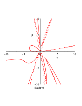
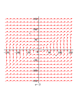
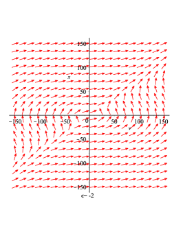
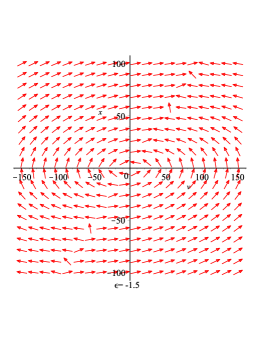
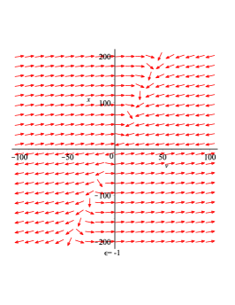
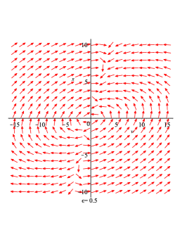
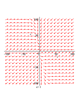
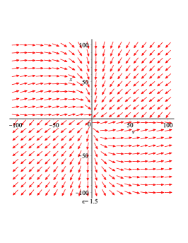
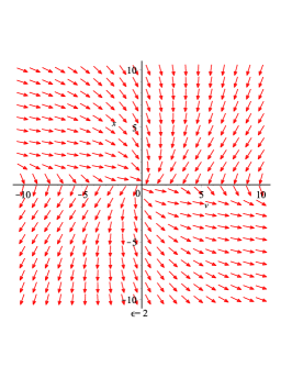
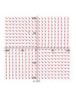
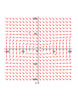
Figure 1: Arrow diagrams for de Sitter inflationary phase for $A_{\|}\neq 0,A_{\perp}=0$. The arrows in the diagram show stable attraction points.

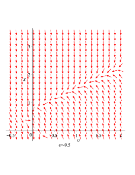
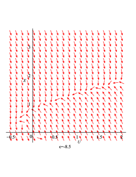
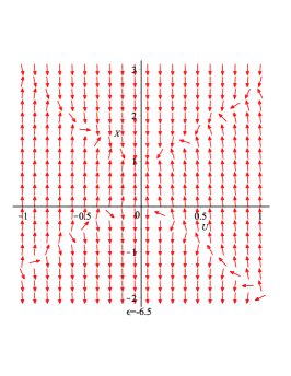
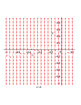
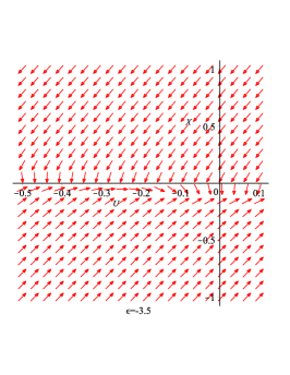
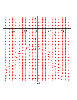
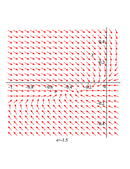
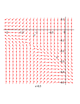
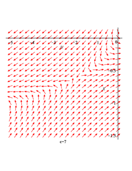
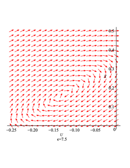
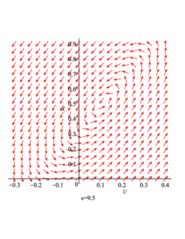
Figure 2: Arrow diagrams for de Sitter inflationary phase for $A_{\|}=0,A_{\perp}\neq 0$. The arrows in the diagram show stable attraction points.

Appendix I

We obtain the EM tensor field (3.2) as follows. At the first step we choose a local coordinate transformation

$$d\tilde{t}=dt,~{}~{}~{}d\tilde{x}=e^{a-2b}dx,~{}~{}~{}d\tilde{y}=e^{a+b}dy,~{}~{}~{}d\tilde{z}=e^{a+b}dz$$ (5.1)

in which the coordinates $(\tilde{t},\tilde{x},\tilde{y},\tilde{z})$ are characterized by a flat Minkonski space time $ds^{2}=-d\tilde{t}^{2}+d\tilde{x}^{2}+d\tilde{y}^{2}+d\tilde{z}^{2}$ for which

$$F_{\tilde{\mu}\tilde{\nu}}=\left(\begin{array}[]{cccc}0&-E_{\tilde{x}}&-E_{\tilde{y}}&-E_{\tilde{z}}\\ E_{\tilde{x}}&0&B_{\tilde{z}}&-B_{\tilde{y}}\\ E_{\tilde{y}}&-B_{\tilde{z}}&0&B_{\tilde{x}}\\ E_{\tilde{z}}&B_{\tilde{y}}&-B_{\tilde{x}}&0\\ \end{array}\right)$$ (5.2)

is well known but the coordinates $(t,x,y,z)$ correspond to the background metric (3.1). At the second step we apply (5.1) to transform (5.2) as $F_{\alpha\beta}=\frac{\partial x^{\tilde{\mu}}}{\partial x^{\alpha}}\frac{\partial x^{\tilde{\nu}}}{\partial x^{\beta}}F_{\tilde{\mu}\tilde{\nu}}$ which reduces to the equation (3.2) and for simplicity we drop over tilde $`\tilde{~{}}`$ in the indexes in (3.2).

Appendix II

Applying the metric equation (3.1) one can calculate simply the non-vanishing Einstein tensor components $G_{\mu}^{\nu}$ as

$$G^{t}_{t}=3(\dot{a}^{2}-\dot{b}^{2}),$$ (5.3)

$$G^{x}_{x}=3\dot{a}^{2}+6\dot{a}\dot{b}+3\dot{b}^{2}+2\ddot{a}+2\ddot{b},$$ (5.4)

$$G^{y}_{y}=G^{z}_{z}=3\dot{a}^{2}-3\dot{a}\dot{b}+3\dot{b}^{2}+2\ddot{a}-\ddot{b}$$ (5.5)

for which the Ricci scalar is

$$R=-12\dot{a}^{2}-6\dot{b}^{2}-6\ddot{a}$$ (5.6)

and for the stress tensors (2.6), (2.7) and (2.8) we obtain respectively

$$T^{t~{}(EM)}_{t}=\frac{1}{4}\{E^{2}+B^{2}\},$$ (5.7)

$$T^{x~{}(EM)}_{x}=\frac{1}{2}\{E_{x}^{2}+B_{x}^{2}\}-\frac{1}{4}\{E^{2}+B^{2}\},$$ (5.8)

$$T^{y~{}(EM)}_{y}=\frac{1}{2}\{E_{y}^{2}+B_{y}^{2}\}-\frac{1}{4}\{E^{2}+B^{2}\},$$ (5.9)

$$T^{z~{}(EM)}_{z}=\frac{1}{2}\{E_{z}^{2}+B_{z}^{2}\}-\frac{1}{4}\{E^{2}+B^{2}\},$$ (5.10)

$$T^{(EM)}_{tx}=e^{a-2b}\frac{S_{x}}{2},~{}~{}~{}T^{(EM)}_{ty}=e^{a+b}\frac{S_{y}}{2},~{}~{}~{}T^{(EM)}_{tz}=e^{a+b}\frac{S_{z}}{2}$$ (5.11)

where

$$~{}~{}~{}\vec{S}=\vec{E}\times\vec{B}$$ (5.12)

is the poynting vector and for both components of the stress tensor $W_{\mu\nu}$ referred by $\|,\perp$, we obtain their relationship with the $\theta_{\mu\nu}$ components as follows.

$$W_{tt}=-e^{-6a}\frac{d}{dt}[e^{3a}\frac{d}{dt}(e^{3a}\theta_{tt})]-2(\dot{a}-2\dot{b})e^{-2a+4b}[\dot{\theta}_{xx}+(\dot{a}+4\dot{b})\theta_{xx}]$$ (5.13)

$$-2(\dot{a}+\dot{b})e^{-2(a+b)}[(\dot{a}-2\dot{b})(\theta_{yy}+\theta_{zz})+\dot{\theta}_{yy}+\dot{\theta}_{zz}]$$

$$W_{xx}=2e^{-6a}\frac{d}{dt}[(\dot{a}-2\dot{b})e^{8a-4b}\theta_{tt}+(\dot{a}-2\dot{b})e^{6a}\theta_{xx}]-4(\dot{a}-2\dot{b})$$ (5.14)

$$\times[(\dot{a}-2\dot{b})e^{2a-4b}\theta_{tt}+\dot{\theta}_{xx}+2(\dot{a}+\dot{b})\theta_{xx}]$$

$$W_{yy}=e^{-6a}\frac{d}{dt}[e^{6a}\dot{\theta}_{yy}+3\dot{a}e^{6a}\theta_{yy}+2(\dot{a}+\dot{b})e^{8a+2b}\theta_{tt}]$$ (5.15)

$$-4(\dot{a}+\dot{b})[\dot{\theta}_{yy}+(2\dot{a}-\dot{b})\theta_{yy}+(\dot{a}+\dot{b})e^{2(a+b)}\theta_{tt}]$$

and

$$W_{zz}=e^{-6a}\frac{d}{dt}[e^{6a}\dot{\theta}_{zz}+3\dot{a}e^{6a}\theta_{zz}+2(\dot{a}+\dot{b})e^{8a+2b}\theta_{tt}]$$ (5.16)

$$-4(\dot{a}+\dot{b})[\dot{\theta}_{zz}+(2\dot{a}-\dot{b})\theta_{zz}+(\dot{a}+\dot{b})e^{2(a+b)}\theta_{tt}]$$

By looking at the above equations we obtain for EM field stress tensor

$$T_{t}^{t(EM_{||})}=\frac{1}{4}({E_{||}^{2}+B^{2}_{||}}),~{}~{}~{}~{}T_{t}^{t(EM_{\perp})}=\frac{1}{2}(E^{2}_{\perp}+B^{2}_{\perp})$$ (5.17)

$$T_{x}^{x(EM_{||})}=\frac{1}{4}({E_{||}^{2}+B^{2}_{||}}),~{}~{}~{}~{}T_{x}^{x(EM_{\perp})}=-\frac{1}{2}(E^{2}_{\perp}+B^{2}_{\perp})$$ (5.18)

$$T_{y}^{y(EM_{||})}=-\frac{1}{4}({E_{||}^{2}+B^{2}_{||}})=T_{z}^{z(EM_{||})},~{}~{}~{}~{}T_{y}^{y(EM_{\perp})}=0=T_{z}^{z(EM_{\perp})}$$ (5.19)

$$T_{tx}^{(EM_{||,\perp})}=0=T_{ty}^{(EM_{||,\perp})}=T_{tz}^{(EM_{||,\perp})}$$ (5.20)

Also we obtain for the vector $P^{\mu}$ and the tensor $\theta^{\mu\nu}$ fields :

$$\theta_{||}^{tt}=-\alpha e^{-2a+4b}A_{||}^{2},~{}~{}~{}\theta_{\perp}^{tt}=-2\alpha e^{-2a-2b}A^{2}_{\perp}$$ (5.21)

$$\theta_{||}^{xx}=(\alpha+\beta)e^{-4a+8b}A_{||}^{2},~{}~{}~{}\theta_{\perp}^{xx}=2\alpha e^{-4a+2b}A^{2}_{\perp}$$ (5.22)

$$\theta_{||}^{yy}=\alpha e^{-4a-4b}A_{||}^{2}=\theta^{zz}_{||},~{}~{}~{}\theta_{\perp}^{yy}=(2\alpha+\beta)e^{-4a-4b}A^{2}_{\perp}=\theta^{zz}_{\perp}$$ (5.23)

$$P^{t}_{||}=-2\alpha A_{||}\dot{A}_{||}e^{-2a+4b}+\{2\alpha(\dot{a}+\dot{b})e^{-2(a+b)}-4\alpha(\dot{a}+\dot{b})e^{-2a+4b}$$ (5.24)

$$+(\alpha+\beta)(\dot{a}-2\dot{b})e^{-6a+4b}\}A_{||}^{2}$$

$$P^{t}_{\perp}=-4\alpha A_{\perp}\dot{A}_{\perp}e^{-2(a+b)}+\{2[(\beta-2\alpha)\dot{a}+(\beta+4\alpha)\dot{b}]e^{-2(a+b)}$$

$$+2\alpha(\dot{a}-2\dot{b})e^{-2(3a+b)}\}A^{2}_{\perp}$$ (5.25)

and

$$P^{x,y,z}_{{||,\perp}}=0$$ (5.26)

$$\nabla_{\xi}P^{\xi}_{||}=-2\alpha e^{-2a+4b}\{\dot{A}_{||}^{2}+A_{||}\ddot{A}_{||}+(5\dot{a}+8\dot{b})A_{||}\dot{A_{||}}\}$$ (5.27)

$$+2\alpha e^{-2a+2b}\{(\ddot{a}+\ddot{b}+\dot{a}^{2}+3\dot{a}\dot{b}+2\dot{b}^{2})A^{2}_{||}+2(\dot{a}+\dot{b})A_{||}\dot{A}_{||}\}$$

$$+(\alpha+\beta)e^{-6a+4b}\{(\ddot{a}-2\ddot{b}-3\dot{a}^{2}+10\dot{a}\dot{b}-8\dot{b}^{2})A^{2}_{||}+2(\dot{a}-2\dot{b})A_{||}\dot{A}_{||}\}$$

and

$$\nabla_{\xi}P_{\perp}^{\xi}=e^{-2(a+b)}\{-4\alpha(\dot{A}^{2}_{\perp}+A_{\perp}\ddot{A}_{\perp})$$ (5.28)

$$+4A_{\perp}\dot{A}_{\perp}[(\beta-3\alpha)\dot{a}+(\beta+6\alpha)\dot{b}]+A^{2}_{\perp}[2(\beta-2\alpha)\ddot{a}+2(\beta+4\alpha)\ddot{b}$$

$$+2(\beta-2\alpha)\dot{a}^{2}+2(8\alpha-\beta)\dot{a}\dot{b}-4(\beta+4\alpha)\dot{b}^{2}]\}$$

$$+2\alpha e^{-2(3a+b)}\{2(\dot{a}-2\dot{b})A_{\perp}\dot{A}_{\perp}+A^{2}_{\perp}(\ddot{a}-2\ddot{b}-3\dot{a}^{2}+4\dot{a}\dot{b}+4\dot{b}^{2})\}.$$

For components of the stress tensors $W^{\|}_{\mu\nu}$ and $W^{\perp}_{\mu\nu}$ we obtain

$$W^{||}_{tt}=2\alpha e^{10a+4b}(\dot{A}^{2}_{||}+A_{||}\ddot{A}_{||})$$ (5.29)

$$+\{\alpha e^{10a+4b}(\ddot{a}+4\ddot{b}+4\dot{a}^{2}+20\dot{a}\dot{b}+16\dot{b}^{2})-2(\alpha+\beta)e^{-2a+4b}(\dot{a^{2}}+2\dot{a}\dot{b}-8\dot{b}^{2})$$

$$-4\alpha e^{-2(a+b)}(\dot{a}^{2}-\dot{a}\dot{b}-2\dot{b}^{2})\}A_{||}^{2}+\{2\alpha e^{10a+4b}(5\dot{a}+8\dot{b})$$

$$-4(\alpha+\beta)(\dot{a}-2\dot{b})e^{-2a+4b}-8\alpha(\dot{a}+\dot{b})e^{-2(a+b)}\}A_{||}\dot{A}_{||}$$

$$W^{\perp}_{tt}=e^{-2(a+b)}\{4\alpha(\dot{A}_{\perp}^{2}+A_{\perp}\ddot{A}_{\perp})$$ (5.30)

$$-2[2(\alpha+2\beta)\dot{a}+(2\alpha+\beta)\dot{b}]A_{\perp}\dot{A}_{\perp}$$

$$+[2\alpha\ddot{a}-4\alpha\ddot{b}-4(\alpha+\beta)\dot{a}^{2}+4(\beta-\alpha)\dot{a}\dot{b}+8(\alpha+\beta)\dot{b}^{2}]A_{\perp}^{2}\}$$

$$W^{||}_{xx}=-4(2\alpha+\beta)(\dot{a}+2\dot{b})A_{||}\dot{A}_{||}+\{2\beta(\ddot{a}-2\ddot{b})$$ (5.31)

$$+4(\beta-\alpha)\dot{a}^{2}-8(\alpha+2\beta)\dot{a}\dot{b}+16(2\alpha+\beta)\dot{b}^{2}\}A^{2}_{||}$$

$$W^{\perp}_{xx}=8\alpha e^{-6b}\{2(2\dot{b}-\dot{a})A_{\perp}\dot{A}_{\perp}+(5\dot{a}^{2}-14\dot{a}\dot{b}+8\dot{b}^{2})A^{2}_{\perp}\}$$ (5.32)

$$W^{||}_{yy}=W^{||}_{zz}=2\alpha[9\dot{a}-2(\dot{a}+\dot{b})e^{6a}]A_{||}\dot{A}_{||}+2\alpha\dot{A}^{2}_{||}+2\alpha A_{||}\ddot{A}_{||}$$ (5.33)

$$+\alpha\{3\ddot{a}+18\dot{a}^{2}-2e^{6a}[\ddot{a}+\ddot{b}+12\dot{a}\dot{b}+12\dot{a}^{2}]\}A_{||}^{2}$$

and

$$W^{\perp}_{yy}=W^{\perp}_{zz}=2\{4(\alpha+\beta)\dot{b}+(22\alpha+13\beta)\dot{a}\}A_{\perp}\dot{A}_{\perp}$$ (5.34)

$$+\{(2\alpha+3\beta)\ddot{a}-4\alpha\ddot{b}+2(2\alpha+5\beta)\dot{a}^{2}+4(\beta+4\alpha)\dot{b}(\dot{b}-\dot{a})\}A_{\perp}^{2}$$

By substituting the above relations into the equation (4.8) we obtain for the directional barotropic indexes $\gamma_{\|}$ and $\gamma_{\perp}$ respectively

$$\alpha[(1+\gamma_{\|})e^{-12a}+\gamma_{\|}]\ddot{v}$$

$$+[\alpha(2-\gamma_{\|})e^{-12a-2b}+(6\alpha+\beta)e^{-12a}+(\alpha+\beta)(1-\gamma_{\|})e^{-16a}-\alpha\gamma_{\|}/2]\ddot{a}$$

$$+[\alpha(2-\gamma_{\|})e^{-12a-2b}-(\alpha+\beta)(2-\gamma_{\|})e^{-16a}+2\beta e^{-12a}-2\alpha\gamma_{\|}]\ddot{b}+([[(9\alpha+2\beta)$$

$$+\gamma_{\|}(7\alpha+2\beta)]\dot{a}+4[(4\alpha+\beta)-\gamma_{\|}(\beta-\alpha)]\dot{b}]e^{-12a}$$

$$+2\alpha(2-\gamma_{\|})(\dot{a}+\dot{b})e^{-12a-2b}+2(\alpha+\beta)(\dot{a}-2\dot{b})e^{-16a}-\gamma_{\|}(\alpha+\beta)(\dot{a}-2\dot{b})$$

$$-\gamma_{\|}\alpha(5\dot{a}+8\dot{b})+4\gamma_{\|}\alpha(\dot{a}+\dot{b})e^{-12a-6b})\dot{v}+e^{-12a}[2\alpha(1+2\gamma_{\|})-(\gamma_{\|}+1)/8]\dot{v}^{2}$$

$$+\{\alpha(2-\gamma_{\|})e^{-12a-2b}+[14\alpha-2\beta+\gamma_{\|}(\alpha+\beta)]e^{-12a}$$

$$-3(\alpha+\beta)(1-\gamma_{\|}/2)e^{-16a}$$

$$-2\alpha\gamma_{\|}+2\alpha\gamma_{\|}e^{-12a-6b}\}\dot{a}^{2}+\{2\alpha(2-\gamma_{\|})e^{-12a-2b}$$

$$-[10\alpha+8\beta+8\gamma_{\|}(\alpha+\beta)]e^{-12a}+4\gamma_{\|}(\alpha+\beta)e^{-16a}-8\alpha\gamma_{\|}$$

$$-4\alpha\gamma_{\|}e^{-12a-6b}\}\dot{b}^{2}+\{3\alpha(2-\gamma_{\|})e^{-12a-2b}+5(\alpha+\beta)(2-\gamma_{\|})e^{-16a}$$

$$+2(\alpha+\beta)(2+\gamma_{\|})e^{-12a}-\alpha\gamma_{\|}-2\alpha\gamma_{\|}e^{-12a-6b}\}\dot{a}\dot{b}=0$$ (5.35)

and

$$\alpha\{(1+\gamma_{\perp})e^{-12a}-e^{-12a-6b}+\gamma_{\perp}\}\ddot{v}$$

$$-\{\alpha(\gamma_{\perp}+1)e^{-12a-2b}+(\alpha+\beta)(1-\gamma_{\perp}/2)e^{-16a}-3\alpha e^{-12a-6b}/2+\alpha e^{-6a-6b}$$

$$-\alpha\gamma_{\perp}/2\}\ddot{a}+\{\alpha e^{-6a-6b}+(1+\gamma_{\perp})(\alpha+\beta)e^{-16a}-\alpha(1+\gamma_{\perp})e^{-12a-2b}$$

$$-2\alpha\gamma_{\perp}\}\ddot{b}+\{[(\alpha(5+\gamma_{\perp})+2\beta\gamma_{\perp})\dot{a}+(4\alpha(2+\gamma_{\perp})-4\beta\gamma_{\perp})\dot{b}]e^{-12a}\}\dot{v}$$

$$+\{[(1-\gamma_{\perp})/8+2\alpha(1+\gamma_{\perp})]e^{-12a}-2\alpha e^{-12a-6b}+2\alpha\gamma_{\perp}\}\dot{v}^{2}$$

$$+\{12\alpha e^{-6a-6b}-\alpha(\gamma_{\perp}+1)e^{-12a-2b}+3(\alpha+\beta)(1+\gamma_{\perp})e^{-16a}/2-2\alpha\gamma_{\perp}$$

$$+\gamma_{\perp}(\alpha+\beta)e^{-12a}-\alpha(9-2\gamma_{\perp})e^{-12a-6b}\}\dot{a}^{2}+\{4(\alpha+\beta)(1+\gamma_{\perp})e^{-16a}$$

$$-2\alpha(\gamma_{\perp}+1)e^{-12a-2b}-8\alpha\gamma_{\perp}-8\gamma_{\perp}(\alpha+\beta)e^{-12a}-4\alpha\gamma_{\perp}e^{-12a-6b}\}\dot{b}^{2}$$

$$+\{12\alpha e^{-6a-6b}-5(\gamma_{\perp}+1)(\alpha+\beta)e^{-16a}-3\alpha(\gamma_{\perp}+1)e^{-12a-2b}-\alpha\gamma_{\perp}$$

$$+2\gamma_{\perp}(\alpha+\beta)e^{-12a}-2\alpha\gamma_{\perp}e^{-12a-6b}\}\dot{a}\dot{b}=0$$ (5.36)

respectively for case $(A_{\|}\neq 0,A_{\perp}=0)$ and

$$2\alpha\ddot{u}+[2\alpha-\beta+\gamma_{\|}(\alpha-\beta)]\ddot{a}$$

$$-[\beta+4\alpha+\gamma_{\|}(\beta+2\alpha)]\ddot{b}+[4\alpha+1/4-\gamma_{\|}/8]\dot{u}^{2}$$

$$+[14\alpha-2\beta+2(4\alpha+\beta)\gamma_{\|}]\dot{a}\dot{u}-[28\alpha+2\beta+\gamma_{\|}(14\alpha+\beta)]\dot{u}\dot{b}+[\beta+48\alpha$$

$$-\gamma_{\|}(\beta+6\alpha)]\dot{a}\dot{b}-[\beta+18\alpha-\gamma_{\|}(\beta+4\alpha)]\dot{a}^{2}+[2\beta-24\alpha+2(2\alpha-\beta)\gamma_{\|}]\dot{b}^{2}$$

$$\alpha(2-\gamma_{\|})e^{-2(2a+b)}[2\dot{u}(\dot{a}-2\dot{b})+\ddot{a}-2\ddot{b}-3\dot{a}^{2}+4\dot{a}\dot{b}+4\dot{b}^{2}]=0$$ (5.37)

and

$$2\alpha\ddot{u}+[7\alpha-5\beta/2+\gamma_{\perp}(\alpha-\beta)]\ddot{a}-(\beta+2\alpha)(1+\gamma_{\perp})\ddot{b}$$

$$+[3\beta-\gamma_{\perp}(6\alpha+\beta)]\dot{a}\dot{b}+[17\alpha-17\beta/2+\gamma_{\perp}(2\beta+8\alpha)]\dot{u}\dot{a}$$

$$-[16\alpha+6\beta+\gamma_{\perp}(14\alpha+\beta)]\dot{u}\dot{b}+(4\alpha-\gamma_{\perp}/8)\dot{u}^{2}$$

$$+[12\alpha-6\beta+\gamma_{\perp}(\beta+4\alpha)]\dot{a}^{2}+[6\alpha+2\gamma_{\perp}(2\alpha-\beta)]\dot{b}^{2}$$

$$+\alpha(2-\gamma_{\perp})e^{-4a}[2\dot{u}(\dot{a}-2\dot{b})+\ddot{a}-2\ddot{b}-3\dot{a}^{2}+4\dot{a}\dot{b}+4\dot{b}^{2}]=0$$ (5.38)

respectively for case $A_{\|}=0,A_{\perp}\neq 0.$ The above equations in limits $e^{a(t)}>>1$ reduce to the simpler forms given by the equations (4.9) and (4.10) respectively for $A_{\|}\neq 0,A_{\perp}=0$ and (4.11) and (4.12) respectively for $A_{\|}=0,A_{\perp}\neq 0.$

Appendix III

The coefficients of the dynamical equations (4.15) and (4.16) are obtained respectively as follows.

$$C_{VV}=2(3168\alpha^{4}+504\alpha^{3}\beta-244\alpha^{2}\beta^{2}-78\alpha\beta^{3}-5\beta^{4}+324\alpha^{3}+432\alpha^{2}\beta$$

$$-9\alpha\beta^{2})/(6\alpha+\beta)^{2}(-6\alpha^{2}+28\alpha\beta+5\beta^{2})$$ (5.39)

$$C_{XV}=-4(1728\alpha^{4}+1584\alpha^{3}\beta-426\alpha^{2}\beta^{2}-80\alpha\beta^{3}-1404\alpha^{3}+198\alpha^{2}\beta$$

$$+102\alpha\beta^{2}+5\beta^{3})/(6\alpha+\beta)^{2}(-6\alpha^{2}+28\alpha\beta+5\beta^{2})$$ (5.40)

and

$$C_{XX}=-\frac{36(324\alpha^{4}-324\alpha^{3}\beta+99\alpha^{2}\beta^{2}-21\alpha\beta^{3}-5\beta^{4})}{(6\alpha+\beta)^{2}(-6\alpha^{2}+28\alpha\beta+5\beta^{2})}$$ (5.41)

$$D_{VV}=(2736\alpha^{4}+1112\alpha^{3}\beta+180\alpha^{2}\beta^{2}+10\alpha\beta^{3}+288\alpha^{3}$$

$$+420\beta^{2}\beta+40\alpha\beta^{2}-\beta^{3})/(6\alpha+\beta)^{2}(-6\alpha^{2}+28\alpha\beta+5\beta^{2})$$ (5.42)

$$D_{XV}=-4(864\alpha^{4}+336\alpha^{3}\beta-112\alpha^{2}\beta^{2}-21\alpha\beta^{3}-612\alpha^{3}-42\alpha^{2}\beta$$

$$+28\alpha\beta^{2}+3\beta^{3})/(6\alpha+\beta)^{2}(-6\alpha^{2}+28\alpha\beta+5\beta^{2})$$ (5.43)

and

$$D_{XX}=-\frac{18(216\alpha^{4}+84\alpha^{3}\beta+110\alpha^{2}\beta^{2}+\alpha\beta^{3}-2\beta^{4})}{(6\alpha+\beta)^{2}(-6\alpha^{2}+28\alpha\beta+5\beta^{2})}.$$ (5.44)

The coefficients in the equation (4.29) have the following forms.

$$\eta_{0}(\epsilon)=-83800\epsilon^{13}-2587010\epsilon^{12}-22948268\epsilon^{11}-60128728\epsilon^{10}$$

$$-212135040\epsilon^{9}-2359178568\epsilon^{8}+3993113808\epsilon^{7}+79174050048\epsilon^{6}$$

$$+16352788032\epsilon^{5}-591326822016\epsilon^{4}+145023084288\epsilon^{3}$$

$$+548045263872\epsilon^{2}-121315304448\epsilon+1451188224$$ (5.45)

$$\eta_{1}(\epsilon)=39500025\epsilon^{14}+341537030\epsilon^{13}-803772011\epsilon^{12}-1532681912\epsilon^{11}$$

$$+35418699464\epsilon^{10}-104741851680\epsilon^{9}+212404729332\epsilon^{8}-307964233008\epsilon^{7}$$

$$-271585335024\epsilon^{6}+1562211831744\epsilon^{5}+1336466034432\epsilon^{4}$$

$$-1089013932288\epsilon^{3}-1111662247680\epsilon^{2}+249154237440\epsilon+6832677888$$ (5.46)

$$\eta_{2}(\epsilon)=377100\epsilon^{15}+9214170\epsilon^{14}+58826066\epsilon^{13}-134067668\epsilon^{12}$$

$$-2199922976\epsilon^{11}-1551871744\epsilon^{10}+35035595592\epsilon^{9}+122344000512\epsilon^{8}$$

$$+101660228064\epsilon^{7}-240137479872\epsilon^{6}-245324163456\epsilon^{5}-2037395172096\epsilon^{4}$$

$$+5424039562752\epsilon^{3}+6649445219328\epsilon^{2}-2625414488064\epsilon$$

$$+214533992448$$ (5.47)

$$\eta_{3}(\epsilon)=900\epsilon^{16}+36180\epsilon^{15}+517209\epsilon^{14}+2130900\epsilon^{13}-22734456\epsilon^{12}$$

$$-321272496\epsilon^{11}-1473018732\epsilon^{10}-847693968\epsilon^{9}+20182695696\epsilon^{8}$$

$$+89619111936\epsilon^{7}+139261389696\epsilon^{6}-18328467456\epsilon^{5}-71728187904\epsilon^{4}$$

$$+910217502720\epsilon^{3}+1721868420096\epsilon^{2}-825967964160\epsilon+89248075776$$ (5.48)

Appendix IV

$$P_{1}=64S^{5}\alpha\epsilon-1136S^{5}\alpha+4S^{5}\epsilon-344S^{4}\alpha\epsilon+28S^{5}+3128S^{4}\alpha-12S^{4}\epsilon$$

$$+292S^{3}\alpha\epsilon-116S^{4}-1592S^{3}\alpha+32S^{3}\epsilon+80S^{2}\alpha\epsilon+176S^{3}-1920S^{2}\alpha-18S^{2}\epsilon$$

$$-356S\alpha\epsilon-44S^{2}+1168S\alpha-4S\epsilon+264\alpha\epsilon-8S+352\alpha+46\epsilon-4$$ (5.49)

$$P_{2}=-128S^{4}\alpha\epsilon+384S^{4}\alpha-20S^{4}\epsilon+16S^{3}\alpha\epsilon-144S^{4}+1056S^{3}\alpha+39S^{3}\epsilon+48S^{2}\alpha\epsilon$$

$$+390S^{3}-2592S^{2}\alpha+39S^{2}\epsilon+272S\alpha\epsilon-354S^{2}+1056S\alpha-3S\epsilon$$

$$-208\alpha\epsilon+90S+96\alpha-55\epsilon+18$$ (5.50)

$$Q_{1}=24576S^{10}\alpha^{3}\epsilon^{2}+3072S^{10}\alpha^{2}\epsilon^{3}+12288S^{9}\alpha^{3}\epsilon^{3}-147456S^{10}\alpha^{3}\epsilon$$

$$-62720S^{10}\alpha^{2}\epsilon^{2}+480S^{10}\alpha\epsilon^{3}-79872S^{9}\alpha^{3}\epsilon^{2}-19968S^{9}\alpha^{2}\epsilon^{3}+9216S^{8}\alpha^{3}\epsilon^{3}$$

$$+221184S^{10}\alpha^{3}-428800S^{10}\alpha^{2}\epsilon-5536S^{10}\alpha\epsilon^{2}-276480S^{9}\alpha^{3}\epsilon+75488S^{9}\alpha^{2}\epsilon^{2}$$

$$-4296S^{9}\alpha\epsilon^{3}-236160S^{8}\alpha^{3}\epsilon^{2}-11792S^{8}\alpha^{2}\epsilon^{3}-12096S^{7}\alpha^{3}\epsilon^{3}+1990720S^{10}\alpha^{2}$$

$$-158240S^{10}\alpha\epsilon+4S^{10}\epsilon^{2}+1216512S^{9}\alpha^{3}+2511936S^{9}\alpha^{2}\epsilon-10600S^{9}\alpha\epsilon^{2}$$

$$+1525248S^{8}\alpha^{3}\epsilon+607064S^{8}\alpha^{2}\epsilon^{2}+3856S^{8}\alpha\epsilon^{3}+242688S^{7}\alpha^{3}\epsilon^{2}+1108S^{7}\alpha^{2}\epsilon^{3}$$

$$-60096S^{6}\alpha^{3}\epsilon^{3}-672544S^{10}\alpha+56S^{10}\epsilon-2697152S^{9}\alpha^{2}+703712S^{9}\alpha\epsilon-24S^{9}\epsilon^{2}$$

$$-870912S^{8}\alpha^{3}-5531872S^{8}\alpha^{2}\epsilon+119672S^{8}\alpha\epsilon^{2}-887040S^{7}\alpha^{3}\epsilon-478080S^{7}\alpha^{2}\epsilon^{2}$$

$$+11016S^{7}\alpha\epsilon^{3}+578688S^{6}\alpha^{3}\epsilon^{2}+41572S^{6}\alpha^{2}\epsilon^{3}-2880S^{5}\alpha^{3}\epsilon^{3}+196S^{10}$$

$$+4037712S^{9}\alpha-400S^{9}\epsilon-15858960S^{8}\alpha^{2}-738904S^{8}\alpha\epsilon+100S^{8}\epsilon^{2}$$

$$-4561920S^{7}\alpha^{3}+1839136S^{7}\alpha^{2}\epsilon-162996S^{7}\alpha\epsilon^{2}-1688832S^{6}\alpha^{3}\epsilon-876292S^{6}\alpha^{2}\epsilon^{2}$$

$$+1336S^{6}\alpha\epsilon^{3}-76032S^{5}\alpha^{3}\epsilon^{2}+10492S^{5}\alpha^{2}\epsilon^{3}+62784S^{4}\alpha^{3}\epsilon^{3}-1624S^{9}$$

$$-10577216S^{8}\alpha+1496S^{8}\epsilon+57504736S^{7}\alpha^{2}-635032S^{7}\alpha\epsilon-228S^{7}\epsilon^{2}$$

$$+10907136S^{6}\alpha^{3}+5613344S^{6}\alpha^{2}\epsilon-193924S^{6}\alpha\epsilon^{2}+523008S^{5}\alpha^{3}\epsilon+128800S^{5}\alpha^{2}\epsilon^{2}$$

$$-8228S^{5}\alpha\epsilon^{3}-903552S^{4}\alpha^{3}\epsilon^{2}+14156S^{4}\alpha^{2}\epsilon^{3}+55104S^{3}\alpha^{3}\epsilon^{3}+5828S^{8}$$

$$+14927136S^{7}\alpha-3252S^{7}\epsilon-75168336S^{6}\alpha^{2}+1035376S^{6}\alpha\epsilon$$

$$+276S^{6}\epsilon^{2}-21897216S^{5}\alpha^{3}+3502272S^{5}\alpha^{2}\epsilon+361200S^{5}\alpha\epsilon^{2}+5831424S^{4}\alpha^{3}\epsilon$$

$$+664112S^{4}\alpha^{2}\epsilon^{2}-932S^{4}\alpha\epsilon^{3}-173568S^{3}\alpha^{3}\epsilon^{2}+10732\S^{3}\alpha^{2}\epsilon^{3}-44352S^{2}\alpha^{3}\epsilon^{3}$$

$$-10824S^{7}-11085888S^{6}\alpha+3492S^{6}\epsilon+36085056S^{5}\alpha^{2}+1569752S^{5}\alpha\epsilon$$

$$+68S^{5}\epsilon^{2}+27993600S^{4}\alpha^{3}-17729664S^{4}\alpha^{2}\epsilon+180476S^{4}\alpha\epsilon^{2}-9305856S^{3}\alpha^{3}\epsilon$$

$$+824000S^{3}\alpha^{2}\epsilon^{2}-7344S^{3}\alpha\epsilon^{3}+1183104S^{2}\alpha^{3}\epsilon^{2}-54884S^{2}\alpha^{2}\epsilon^{3}-52416S\alpha^{3}\epsilon^{3}$$

$$+10184S^{6}+2759264S^{5}\alpha+948S^{5}\epsilon+7933920S^{4}\alpha^{2}-3349368S^{4}\alpha\epsilon-899S^{4}\epsilon^{2}$$

$$-15510528S^{3}\alpha^{3}+10608720S^{3}\alpha^{2}\epsilon$$

$$-252676S^{3}\alpha\epsilon^{2}+5541120S^{2}\alpha^{3}\epsilon-1020020S^{2}\alpha^{2}\epsilon^{2}-10336S^{2}\alpha\epsilon^{3}-659712S\alpha^{3}\epsilon^{2}$$

$$-43836S\alpha^{2}\epsilon^{3}+32448\alpha^{3}\epsilon^{3}-3464S^{5}+1523680S^{4}\alpha-6248S^{4}\epsilon-11764864S^{3}\alpha^{2}$$

$$+1583464S^{3}\alpha\epsilon+1132S^{3}\epsilon^{2}+1866240S^{2}\alpha^{3}+1220976S^{2}\alpha^{2}\epsilon-188892S^{2}\alpha\epsilon^{2}$$

$$-1002240S\alpha^{3}\epsilon-49088S\alpha^{2}\epsilon^{2}+3668S\alpha\epsilon^{3}+99840\alpha^{3}\epsilon^{2}+49348\alpha^{2}\epsilon^{3}+12S^{4}$$

$$-993152S^{3}\alpha+5024S^{3}\epsilon+1157152S^{2}\alpha^{2}+215184S^{2}\alpha\epsilon+70S^{2}\epsilon^{2}+608256S\alpha^{3}$$

$$-1497712S\alpha^{2}\epsilon+108272S\alpha\epsilon^{2}-112896\alpha^{3}\epsilon+186736\alpha^{2}\epsilon^{2}+10780\alpha\epsilon^{3}-176S^{3}$$

$$+21520S^{2}\alpha-800S^{2}\epsilon+756224S\alpha^{2}-205096S\alpha\epsilon-1012S\epsilon^{2}+27648\alpha^{3}$$

$$-108336\alpha^{2}\epsilon+45004\alpha\epsilon^{2}+104S^{2}+55440S\alpha-96S\epsilon+61504\alpha^{2}-20848\alpha\epsilon+$$

$$529\epsilon^{2}+16S+4048\alpha-92\epsilon+4$$ (5.51)

$$Q_{2}=6144S^{10}\alpha^{3}\epsilon^{5}-253952S^{10}\alpha^{3}\epsilon^{4}+8160S^{10}\alpha^{2}\epsilon^{5}-105216S^{9}\alpha^{3}\epsilon^{5}$$

$$-1902592S^{10}\alpha^{3}\epsilon^{3}-234400S^{10}\alpha^{2}\epsilon^{4}-430336S^{9}\alpha^{3}\epsilon^{4}-133896S^{9}\alpha^{2}\epsilon^{5}$$

$$-119296S^{8}\alpha^{3}\epsilon^{5}+8212480S^{10}\alpha^{3}\epsilon^{2}-6215936S^{10}\alpha^{2}\epsilon^{3}+1156S^{10}\alpha\epsilon^{4}$$

$$+10249728S^{9}\alpha^{3}\epsilon^{3}-2447320S^{9}\alpha^{2}\epsilon^{4}+2077696S^{8}\alpha^{3}\epsilon^{4}-261808S^{8}\alpha^{2}\epsilon^{5}$$

$$+57728S^{7}\alpha^{3}\epsilon^{5}+13541376S^{10}\alpha^{3}\epsilon-40224640S^{10}\alpha^{2}\epsilon^{2}+22712S^{10}\alpha\epsilon^{3}$$

$$+7140352S^{9}\alpha^{3}\epsilon^{2}-8378320S^{9}\alpha^{2}\epsilon^{3}-16728S^{9}\alpha\epsilon^{4}-9789184S^{8}\alpha^{3}\epsilon^{3}$$

$$-1721008S^{8}\alpha^{2}\epsilon^{4}-132864S^{7}\alpha^{3}\epsilon^{4}+27588S^{7}\alpha^{2}\epsilon^{5}+403712S^{6}\alpha^{3}\epsilon^{5}$$

$$+3686400S^{10}\alpha^{3}-81907200S^{10}\alpha^{2}\epsilon+131956S^{10}\alpha\epsilon^{2}+3373056\S^{9}\alpha^{3}\epsilon$$

$$+36944736S^{9}\alpha^{2}\epsilon^{2}-379240S^{9}\alpha\epsilon^{3}-40166400S^{8}\alpha^{3}\epsilon^{2}-4043304S^{8}\alpha^{2}\epsilon^{3}$$

$$+4652S^{8}\alpha\epsilon^{4}-528896S^{7}\alpha^{3}\epsilon^{3}+1689368S^{7}\alpha^{2}\epsilon^{4}-2399232S^{6}\alpha^{3}\epsilon^{4}$$

$$+517248S^{6}\alpha^{2}\epsilon^{5}$$

$$+188672S^{5}\alpha^{3}\epsilon^{5}-47655936S^{10}\alpha^{2}+200400S^{10}\alpha\epsilon-1474560S^{9}\alpha^{3}$$

$$+124048320S^{9}\alpha^{2}\epsilon$$

$$-2579920S^{9}\alpha\epsilon^{2}-24013824S^{8}\alpha^{3}\epsilon-90626336S^{8}\alpha^{2}\epsilon^{2}+448128S^{8}\alpha\epsilon^{3}$$

$$+135737344S^{7}\alpha^{3}\epsilon^{2}+7465024S^{7}\alpha^{2}\epsilon^{3}-71364S^{7}\alpha\epsilon^{4}+5481728S^{6}\alpha^{3}\epsilon^{3}$$

$$+2902864S^{6}\alpha^{2}\epsilon^{4}-256S^{5}\alpha^{3}\epsilon^{4}+429496S^{5}\alpha^{2}\epsilon^{5}-253568S^{4}\alpha^{3}\epsilon^{5}$$

$$+90000S^{10}\alpha$$

$$+60042240S^{9}\alpha^{2}-5098560S^{9}\alpha\epsilon+7520256S^{8}\alpha^{3}-239536416S^{8}\alpha^{2}\epsilon$$

$$+4928264S^{8}\alpha\epsilon^{2}+69556224S^{7}\alpha^{3}\epsilon+61286304S^{7}\alpha^{2}\epsilon^{2}-413444S^{7}\alpha\epsilon^{3}$$

$$-232470528S^{6}\alpha^{3}\epsilon^{2}+6333656S^{6}\alpha^{2}\epsilon^{3}-45008S^{6}\alpha\epsilon^{4}+12833280S^{5}\alpha^{3}\epsilon^{3}$$

$$+2968136S^{5}\alpha^{2}\epsilon^{4}+1385728S^{4}\alpha^{3}\epsilon^{4}-51716S^{4}\alpha^{2}\epsilon^{5}-285568S^{3}\alpha^{3}\epsilon^{5}$$

$$-2881152S^{9}\alpha-97712640S^{8}\alpha^{2}+12139536S^{8}\alpha\epsilon+576S^{8}\epsilon^{2}$$

$$-2949120S^{7}\alpha^{3}+184487616S^{7}\alpha^{2}\epsilon+3377376S^{7}\alpha\epsilon^{2}$$

$$+576S^{7}\epsilon^{3}-137892864S^{6}\alpha^{3}\epsilon+41340800S^{6}\alpha^{2}\epsilon^{2}-1515888S^{6}\alpha\epsilon^{3}$$

$$+146562048S^{5}\alpha^{3}\epsilon^{2}+21912144S^{5}\alpha^{2}\epsilon^{3}+176488S^{5}\alpha\epsilon^{4}-43125504S^{4}\alpha^{3}\epsilon^{3}$$

$$+1574072S^{4}\alpha^{2}\epsilon^{4}+1281792S^{3}\alpha^{3}\epsilon^{4}-301452S^{3}\alpha^{2}\epsilon^{5}-35584S^{2}\alpha^{3}\epsilon^{5}$$

$$+8660160S^{8}\alpha+5760S^{8}\epsilon+98878464S^{7}\alpha^{2}$$

$$+19415424S^{7}\alpha\epsilon+5760S^{7}\epsilon^{2}-10764288S^{6}\alpha^{3}$$

$$+46298528S^{6}\alpha^{2}\epsilon-12410180S^{6}\alpha\epsilon^{2}+2304S^{6}\epsilon^{3}+115292160S^{5}\alpha^{3}\epsilon$$

$$+44002656S^{5}\alpha^{2}\epsilon^{2}+353992S^{5}\alpha\epsilon^{3}-13218816S^{4}\alpha^{3}\epsilon^{2}-8373416S^{4}\alpha^{2}\epsilon^{3}$$

$$+205437S^{4}\alpha\epsilon^{4}+29578752S^{3}\alpha^{3}\epsilon^{3}-1545016S^{3}\alpha^{2}\epsilon^{4}-2917376S^{2}\alpha^{3}\epsilon^{4}$$

$$-217224S^{2}\alpha^{2}\epsilon^{5}+61440S\alpha^{3}\epsilon^{5}+5184S^{8}+22019616S^{7}\alpha-8064S^{7}\epsilon$$

$$-14608896S^{6}\alpha^{2}-36238000S^{6}\alpha\epsilon+19008S^{6}\epsilon^{2}+4423680S^{5}\alpha^{3}$$

$$-5504064S^{5}\alpha^{2}\epsilon-3138432S^{5}\alpha\epsilon^{2}$$

$$+3456S^{5}\epsilon^{3}-51391488S^{4}\alpha^{3}\epsilon-75845920S^{4}\alpha^{2}\epsilon^{2}+1633188S^{4}\alpha\epsilon^{3}$$

$$-25483264S^{3}\alpha^{3}\epsilon^{2}-1767488S^{3}\alpha^{2}\epsilon^{3}+4168S^{3}\alpha\epsilon^{4}-3055872S^{2}\alpha^{3}\epsilon^{3}$$

$$-2991008S^{2}\alpha^{2}\epsilon^{4}+1217024S\alpha^{3}\epsilon^{4}-68136S\alpha^{2}\epsilon^{5}+81536\alpha^{3}\epsilon^{5}-17280S^{7}$$

$$-32894400S^{6}\alpha+55296S^{6}\epsilon-28480512S^{5}\alpha^{2}-11973200S^{5}\alpha\epsilon-56736S^{5}\epsilon^{2}$$

$$-15187968S^{4}\alpha^{3}-98371104S^{4}\alpha^{2}\epsilon+3873668S^{4}\alpha\epsilon^{2}+16416S^{4}\epsilon^{3}$$

$$-22984704S^{3}\alpha^{3}\epsilon+12038560S^{3}\alpha^{2}\epsilon^{2}$$

$$+1023168S^{3}\alpha\epsilon^{3}+8101888S^{2}\alpha^{3}\epsilon^{2}-7206168S^{2}\alpha^{2}\epsilon^{3}-75270S^{2}\alpha\epsilon^{4}$$

$$+748544S\alpha^{3}\epsilon^{3}-75920S\alpha^{2}\epsilon^{4}+171776\alpha^{3}\epsilon^{4}+10780\alpha^{2}\epsilon^{5}+12096S^{6}$$

$$-12323904S^{5}\alpha-221472S^{5}\epsilon-16200192S^{4}\alpha^{2}+5234736S^{4}\alpha\epsilon$$

$$+35712S^{4}\epsilon^{2}+5898240S^{3}\alpha^{3}$$

$$+33378368S^{3}\alpha^{2}\epsilon+6822456S^{3}\alpha\epsilon^{2}+8928S^{3}\epsilon^{3}+39736320S^{2}\alpha^{3}\epsilon$$

$$+5423296S^{2}\alpha^{2}\epsilon^{2}-428180S^{2}\alpha\epsilon^{3}+5335040S\alpha^{3}\epsilon^{2}+1540864S\alpha^{2}\epsilon^{3}$$

$$-6396S\alpha\epsilon^{4}-489984\alpha^{3}\epsilon^{3}$$

$$+87592\alpha^{2}\epsilon^{4}-127872S^{5}+5319504S^{4}\alpha-150912S^{4}\epsilon+25857024S^{3}\alpha^{2}$$

$$+15261744S^{3}\alpha\epsilon+127296S^{3}\epsilon^{2}+14155776S^{2}\alpha^{3}+21374816S^{2}\alpha^{2}\epsilon$$

$$-96820S^{2}\alpha\epsilon^{2}-5760S^{2}\epsilon^{3}$$

$$-4657152S\alpha^{3}\epsilon+2878592S\alpha^{2}\epsilon^{2}+65284S\alpha\epsilon^{3}+249856\alpha^{3}\epsilon^{2}+33424\alpha^{2}\epsilon^{3}$$

$$+529\alpha\epsilon^{4}-363456S^{4}+11275968S^{3}\alpha+481248S^{3}\epsilon+6987264S^{2}\alpha^{2}$$

$$+1933504S^{2}\alpha\epsilon-5760S^{2}\epsilon^{2}-5898240S\alpha^{3}$$

$$-1440896S\alpha^{2}\epsilon+269504S\alpha\epsilon^{2}-559104\alpha^{3}\epsilon-290048\alpha^{2}\epsilon^{2}-2104\alpha\epsilon^{3}$$

$$+538560S^{3}+1619968S^{2}\alpha+61920S^{2}\epsilon-4012032S\alpha^{2}$$

$$-313152S\alpha\epsilon+9504S\epsilon^{2}+589824\alpha^{3}-154048\alpha^{2}\epsilon-31360\alpha\epsilon^{2}+116928S^{2}$$

$$-796288S\alpha+8640S\epsilon+316416\alpha^{2}-8000\alpha\epsilon$$

$$-39744S+51904\alpha-2016\epsilon+2304$$ (5.52)

$$K=2S^{3}\alpha^{2}\epsilon^{3}-2S^{3}\alpha^{2}\epsilon^{2}-2S^{3}\alpha\epsilon^{3}+2S^{2}\alpha^{2}\epsilon^{3}-3S^{3}\alpha\epsilon^{2}-2S^{2}\alpha^{2}\epsilon^{2}$$

$$-4S^{2}\alpha\epsilon^{3}-2S\alpha^{2}\epsilon^{3}-76S^{3}\alpha\epsilon+7S^{3}\epsilon^{2}-13S^{2}\alpha\epsilon^{2}+2S\alpha^{2}\epsilon^{2}$$

$$-2S\alpha\epsilon^{3}-2\alpha^{2}\epsilon^{3}-120S^{3}\alpha+S^{3}\epsilon+26S^{2}\alpha\epsilon-2S^{2}\epsilon^{2}+5S\alpha\epsilon^{2}+2\alpha^{2}\epsilon^{2}$$

$$-56S^{3}+24S^{2}\alpha-11S^{2}\epsilon+78S\alpha\epsilon-3S\epsilon^{2}+3\alpha\epsilon^{2}+22S^{2}+120S\alpha+9S\epsilon$$

$$-12\alpha\epsilon+42S-24\alpha+3\epsilon-12$$ (5.53)

we defined

$$J=-4\beta\gamma_{\|}\alpha+2\alpha\beta^{2}\gamma_{\perp}-2\alpha^{2}\gamma_{\|}\gamma_{\perp}$$ (5.54)

$$-2\alpha^{2}\beta\gamma_{\perp}+3\alpha\beta\gamma_{\perp}+\beta^{2}\gamma_{\|}\gamma_{\perp}-30\beta\gamma_{\|}\alpha^{2}-5\alpha\beta^{2}\gamma_{\|}$$

$$+2\alpha^{2}\beta\gamma_{\|}^{2}-\alpha\beta^{2}\gamma_{\|}^{2}-2\alpha^{2}\beta^{2}\gamma_{\|}+2\alpha\beta^{3}\gamma_{\|}+\alpha\beta\gamma_{\|}\gamma_{\perp}+5\beta^{2}\gamma_{\|}/2-18\alpha^{2}\gamma_{\|}$$

$$+\alpha\beta-4\alpha^{2}\gamma_{\perp}+\beta^{2}\gamma_{\perp}-48\alpha^{3}\gamma_{\|}-46\alpha^{2}\beta+\alpha\beta^{2}-\beta^{3}\gamma_{\|}^{2}$$

$$-\beta^{3}\gamma_{\|}-32\alpha^{2}+5\beta^{2}/2-72\alpha^{3}$$

$$E_{1}=(1/2)\alpha^{2}\gamma_{\|}\gamma_{\perp}-(15/4)\alpha\beta\gamma_{\perp}-\beta^{2}\gamma_{\|}\gamma_{\perp}-4\alpha\beta^{2}\gamma_{\perp}-\gamma_{\|}^{2}\beta\alpha+4\alpha^{2}\beta\gamma_{\perp}$$

$$-2\alpha^{2}\beta\gamma_{\|}^{2}+\alpha\beta^{2}\gamma_{\|}^{2}+9\alpha\beta^{2}\gamma_{\|}+(33/8)\alpha\beta\gamma_{\|}+62\alpha^{2}\beta\gamma_{\|}-4\alpha\beta^{3}\gamma_{\|}$$

$$+(1/8)\beta^{3}\gamma_{\|}\gamma_{\perp}+96\alpha^{3}\gamma_{\|}-(3/2)\gamma_{\|}^{2}\alpha^{2}-2\alpha\beta^{2}+92\alpha^{2}\beta$$

$$-(1/8)\gamma_{\|}^{2}\beta^{2}+4\alpha^{2}\beta^{2}\gamma_{\|}+144\alpha^{3}+35\alpha^{2}-(23/8)\beta^{2}$$

$$+\alpha^{2}\gamma_{\perp}-(11/8)\beta^{2}\gamma_{\perp}+\beta^{3}\gamma_{\|}+(11/4)\alpha\beta+\beta^{3}\gamma_{\|}^{2}+(39/2)\alpha^{2}\gamma_{\|}$$

$$-(33/16)\beta^{2}\gamma_{\|}-(1/8)\alpha\beta^{2}\gamma_{\|}\gamma_{\perp}-(17/8)\alpha\beta\gamma_{\|}\gamma_{\perp}$$ (5.55)

$$E_{2}=98\alpha^{2}\beta\gamma_{\perp}+16\alpha\beta^{2}\gamma_{\perp}+5\beta^{3}\gamma_{\|}\gamma_{\perp}-44\alpha^{2}\gamma_{\|}^{2}\beta-12\alpha\gamma_{\|}^{2}\beta^{2}+24\alpha^{3}\beta\gamma_{\|}^{2}$$

$$-6\alpha^{2}\beta^{2}\gamma_{\|}^{2}-15\alpha\beta^{3}\gamma_{\|}^{2}+24\alpha^{3}\beta\gamma_{\|}+6\alpha^{2}\beta^{2}\gamma_{\|}-33\alpha\beta^{3}\gamma_{\|}+6\alpha^{2}\beta\gamma_{\|}-\alpha\beta^{2}\gamma_{\|}$$

$$+24\alpha^{3}\gamma_{\|}\gamma_{\perp}-\beta^{4}\gamma_{\|}\gamma_{\perp}-48\alpha^{3}\gamma_{\|}^{2}$$

$$-\beta^{3}\gamma_{\|}^{2}+120\alpha^{3}+3\beta^{3}\gamma_{\perp}-15\alpha\beta^{2}+150\alpha^{2}\beta+4\beta^{3}\gamma_{\|}+3\beta^{4}\gamma_{\|}+96\alpha^{3}\gamma_{\|}$$

$$-3\beta^{4}\gamma_{\|}^{2}+48\alpha^{3}\gamma_{\perp}-3\alpha\beta^{3}\gamma_{\|}\gamma_{\perp}+4\alpha^{2}\beta^{2}\gamma_{\|}\gamma_{\perp}+30\alpha\beta^{2}\gamma_{\|}\gamma_{\perp}$$

$$+46\alpha^{2}\beta\gamma_{\|}\gamma_{\perp}$$ (5.56)

$$E_{3}=12\alpha^{3}\beta\gamma_{\|}^{2}-6\alpha\beta^{3}\gamma_{\|}^{2}-6\alpha^{2}\beta^{2}\gamma_{\|}^{2}+24\alpha\beta^{2}\gamma_{\perp}-26\alpha^{2}\beta\gamma_{\perp}-12\alpha\beta^{2}\gamma_{\|}\gamma_{\perp}$$

$$+18\alpha^{2}\beta\gamma_{\|}\gamma_{\perp}+12\alpha^{3}\beta\gamma_{\|}-12\alpha\beta^{3}\gamma_{\|}-27\alpha\beta^{2}\gamma_{\|}-140\alpha^{2}\beta\gamma_{\|}+36\alpha^{3}\gamma_{\|}\gamma_{\perp}$$

$$+2\beta^{4}\gamma_{\|}\gamma_{\perp}+8\alpha^{2}\gamma_{\|}^{2}\beta-12\alpha\gamma_{\|}^{2}\beta^{2}+48\alpha^{3}\gamma_{\|}^{2}-2\beta^{3}\gamma_{\|}^{2}+5\beta^{3}\gamma_{\|}-4\beta^{3}\gamma_{\perp}-3\beta^{3}$$

$$-384\alpha^{3}+93\alpha\beta^{2}-324\alpha^{3}\gamma_{\|}-342\alpha^{2}\beta+4\alpha^{2}\beta^{2}\gamma_{\|}\gamma_{\perp}$$

$$-6\alpha\beta^{3}\gamma_{\|}\gamma_{\perp}+72\alpha^{3}\gamma_{\perp}$$ (5.57)

$$E_{4}=12\alpha^{2}\gamma_{\perp}-3\beta^{2}\gamma_{\perp}+96\alpha^{3}\gamma_{\|}^{2}+468\alpha^{3}\gamma_{\|}+118\alpha^{2}\beta-102\alpha\beta^{2}+4\beta^{3}\gamma_{\perp}$$

$$-(21/2)\beta^{3}\gamma_{\|}+5\beta^{3}\gamma_{\|}^{2}+54\alpha^{2}\gamma_{\|}-(15/2)\beta^{2}\gamma_{\|}+8\alpha^{2}\beta^{2}\gamma_{\|}\gamma_{\perp}-6\alpha\beta^{3}\gamma_{\|}\gamma_{\perp}$$

$$-3\alpha\beta\gamma_{\|}\gamma_{\perp}+96\alpha^{2}\gamma_{\|}\beta\gamma_{\perp}+18\alpha\gamma_{\|}\beta^{2}\gamma_{\perp}-(11/2)\beta^{3}+576\alpha^{3}-(15/2)\beta^{2}$$

$$+96\alpha^{2}-2\beta^{4}\gamma_{\|}\gamma_{\perp}+17\alpha^{2}\beta^{2}\gamma_{\|}-(51/2)\alpha\beta^{3}\gamma_{\|}+96\alpha^{3}\gamma_{\|}\gamma_{\perp}+126\alpha^{2}\beta\gamma_{\perp}$$

$$+8\alpha\beta^{2}\gamma_{\perp}+260\alpha^{2}\beta\gamma_{\|}-32\alpha\beta^{2}\gamma_{\|}+27\alpha\beta^{2}\gamma_{\|}^{2}+82\alpha^{2}\beta\gamma_{\|}^{2}+12\alpha\beta\gamma_{\|}$$

$$-3\beta^{2}\gamma_{\|}\gamma_{\perp}+6\alpha^{2}\gamma_{\|}\gamma_{\perp}-9\alpha\beta\gamma_{\perp}-3\alpha\beta+192\alpha^{3}\gamma_{\perp}+(17/2)\beta^{4}\gamma_{\|}$$ (5.58)

$$E_{5}=\beta^{3}\gamma_{\perp}+504\gamma_{\|}\alpha^{3}-72\gamma_{\|}^{2}\alpha^{3}-\gamma_{\|}^{2}\beta^{3}-3\beta^{4}\gamma_{\|}^{2}-6\beta^{4}\gamma_{\|}+708\alpha^{2}\beta$$

$$-30\alpha\beta^{2}+13\beta^{3}\gamma_{\|}-6\alpha^{2}\beta^{2}\gamma_{|}\gamma_{\perp}+5\alpha\beta^{3}\gamma_{\|}\gamma_{\perp}$$

$$-72\alpha^{2}\beta\gamma_{\|}\gamma_{\perp}-6\alpha\beta^{2}\gamma_{\|}\gamma_{\perp}-144\alpha^{3}\gamma_{\perp}+576\alpha^{3}+9\beta^{3}$$

$$-72\alpha^{3}\gamma_{\|}\gamma_{\perp}+\beta^{4}\gamma_{\|}\gamma_{\perp}-60\gamma_{\|}^{2}\alpha^{2}\beta-14\gamma_{\|}^{2}\alpha\beta^{2}+6\alpha^{2}\beta^{2}\gamma_{\|}^{2}-3\alpha\beta^{3}\gamma_{\|}^{2}$$

$$+6\alpha^{2}\beta^{2}\gamma_{\|}+276\alpha^{2}\beta\gamma_{\|}+62\alpha\beta^{2}\gamma_{\|}-36\alpha^{2}\beta\gamma_{\perp}$$

$$-52\alpha\beta^{2}\gamma_{\perp}+3\beta^{3}\gamma_{\|}\gamma_{\perp}$$ (5.59)

$$E_{6}=4\alpha\beta^{2}\gamma_{\perp}-168\alpha^{3}\gamma_{\|}^{2}-696\alpha^{3}\gamma_{\|}-\beta^{3}\gamma_{\|}^{2}-(13/2)\beta^{3}\gamma_{\|}-716\alpha^{2}\beta$$

$$-52\alpha\beta^{2}+\beta^{3}\gamma_{\perp}-14\alpha^{2}\beta^{2}\gamma_{\|}\gamma_{\perp}+13\alpha\beta^{3}\gamma_{\|}\gamma_{\perp}$$

$$-138\alpha^{2}\gamma_{\|}\beta\gamma_{\perp}-9\alpha\gamma_{\|}\beta^{2}\gamma_{\perp}-336\alpha^{3}\gamma_{\perp}+6\beta^{4}\gamma_{\|}-720\alpha^{3}-3\beta^{3}$$

$$-168\alpha^{3}\gamma_{\|}\gamma_{\perp}+\beta^{4}\gamma_{\|}\gamma_{\perp}-16\alpha^{2}\beta^{2}\gamma_{\|}+10\alpha\beta^{3}\gamma_{\|}-124\alpha^{2}\gamma_{\|}^{2}\beta-22\alpha\gamma_{\|}^{2}\beta^{2}$$

$$-670\alpha^{2}\gamma_{\|}\beta-102\alpha\gamma_{\|}\beta^{2}-164\alpha^{2}\beta\gamma_{\perp}$$ (5.60)

$$M_{1}=-(1/4)\alpha\beta\gamma_{\perp}+(17/4)\alpha\beta\gamma_{\|}+12\alpha^{2}+(7/2)\alpha\beta+8\alpha^{2}\gamma_{\|}-(1/8)\gamma_{\|}^{2}\beta$$

$$-(1/4)\alpha\gamma_{\|}\gamma_{\perp}-(1/8)\beta\gamma_{\|}\gamma_{\perp}+(1/2)\alpha-(1/2)\alpha\gamma_{\perp}-(1/8)\beta\gamma_{\perp}-(1/4)\gamma_{\|}^{2}\alpha$$

$$+(1/4)\gamma_{\|}\alpha+(1/8)\gamma_{\perp}\beta+(1/4)\beta$$ (5.61)

$$M_{2}=8\alpha^{2}\beta\gamma_{\perp}+2\alpha\beta^{2}\gamma_{\perp}+80\alpha^{2}\beta\gamma_{\|}+14\alpha\beta^{2}\gamma_{\|}+144\alpha^{3}-2\alpha\beta^{2}$$

$$+72\alpha^{2}\beta+96\alpha^{3}\gamma_{\|}-8\alpha^{2}\gamma_{\|}^{2}+8\alpha^{2}\gamma_{\|}\gamma_{\perp}+8\alpha\beta\gamma_{\perp}+\beta^{2}\gamma_{\|}\gamma_{\perp}+14\alpha\gamma_{\|}\beta$$

$$-6\alpha\gamma_{\|}^{2}\beta+6\alpha\beta\gamma_{\|}\gamma_{\perp}+84\alpha^{2}-\beta^{2}\gamma_{\|}^{2}+16\alpha^{2}\gamma_{\perp}+\beta^{2}\gamma_{\perp}+8\alpha\beta$$

$$-6\beta^{2}\gamma_{\|}+52\alpha^{2}\gamma_{\perp}-5\beta^{2}$$ (5.62)

$$M_{3}=8\alpha^{2}\beta\gamma_{\perp}-4\alpha\beta^{2}\gamma_{\perp}+16\alpha^{2}\beta\gamma_{\|}+4\alpha\beta^{2}\gamma_{\|}-4\alpha\beta^{2}+48\alpha^{3}\gamma_{\|}+92\alpha^{2}\beta$$

$$+8\alpha^{2}\gamma_{\|}^{2}+8\alpha^{2}\gamma_{\|}\gamma_{\perp}-4\alpha\beta\gamma\perp-2\beta^{2}\gamma_{\|}\gamma_{\perp}-18\alpha\gamma_{\|}\beta-32\alpha^{2}+16\alpha^{2}\gamma_{\perp}$$

$$-2\beta^{2}\gamma_{\perp}-18\alpha\beta-2\beta^{2}\gamma_{\perp}^{2}-36\alpha^{2}\gamma_{\|}+2\beta^{2}+72\alpha^{3}$$ (5.63)

$$M_{4}=32\alpha^{2}\gamma_{\perp}+2\beta^{2}\gamma_{\perp}+6\alpha^{2}\beta-13\alpha\beta^{2}+24\alpha^{2}\beta+54\alpha^{2}\gamma_{\|}-19\alpha\beta$$

$$-(17/2)\beta^{2}\gamma_{\|}+12\alpha\beta\gamma_{\|}\gamma_{\perp}-(21/2)\beta^{2}+60\alpha^{2}+16\alpha^{2}\beta\gamma_{\perp}+4\alpha\beta^{2}\gamma_{\perp}$$

$$-16\alpha^{2}\beta\gamma_{\|}-4\alpha\beta^{2}\gamma_{\|}+10\alpha\beta\gamma_{\|}+16\alpha^{2}\gamma_{\|}\gamma_{\perp}+16\alpha\beta\gamma_{\perp}+2\beta^{2}\gamma_{\|}\gamma_{\perp}$$

$$+16\alpha^{2}\gamma_{\|}^{2}+2\beta^{2}\gamma_{\|}^{2}+12\alpha\beta\gamma_{\|}^{2}$$ (5.64)

$$M_{5}=-60\alpha^{2}\beta+16\alpha\beta^{2}+36\alpha^{2}\beta\gamma_{\|}+14\alpha\beta^{2}\gamma_{\|}-12\alpha^{2}\beta\gamma_{\perp}-2\alpha\beta^{2}\gamma_{\perp}$$

$$+96\alpha^{2}-8\alpha\beta\gamma_{\|}\gamma_{\perp}-24\alpha^{2}\gamma_{\perp}-\beta^{2}\gamma_{\perp}+84\alpha^{2}\gamma_{\|}+3\beta^{2}\gamma_{\|}+62\alpha\beta-\beta^{2}\gamma_{\|}^{2}$$

$$+48\alpha\gamma_{\|}\beta-8\alpha\gamma_{\|}^{2}\beta-12\alpha^{2}\gamma_{\|}\gamma_{\perp}-10\alpha\beta\gamma_{\perp}-\beta^{2}\gamma_{\|}\gamma_{\perp}$$

$$+4\beta^{2}-12\gamma_{\|}^{2}\alpha^{2}$$ (5.65)

$$M_{6}=-8\alpha\beta^{2}+28\alpha^{2}\gamma_{\|}\beta+2\alpha\gamma_{\|}\beta^{2}-28\alpha^{2}\beta\gamma_{\perp}-2\alpha\beta^{2}\gamma_{\perp}-120\alpha^{2}$$

$$-16\alpha\beta\gamma_{\|}\gamma_{\perp}-56\alpha^{2}\gamma_{\perp}-\beta^{2}\gamma_{\perp}-9\beta^{2}\gamma_{\|}-72\alpha\beta-\beta^{2}\gamma_{\|}^{2}-76\alpha\gamma_{\|}\beta-16\alpha\gamma_{\|}^{2}\beta$$

$$-28\alpha^{2}\gamma_{\|}\gamma_{\perp}-18\alpha\beta\gamma_{\perp}-\beta^{2}\gamma_{\|}\gamma_{\perp}-8\beta^{2}-116\alpha^{2}\gamma_{\|}-28\alpha^{2}\gamma_{\|}^{2}$$ (5.66)

$$N_{1}=-(7/4)\alpha\beta\gamma_{\perp}+(1/8)\beta^{2}\gamma_{\|}\gamma_{\perp}+2\alpha^{2}\beta\gamma_{\|}-2\alpha\beta^{2}\gamma_{\|}-(1/4)\alpha\beta\gamma_{\|}+13\alpha^{2}$$

$$+(7/2)\alpha^{2}\gamma_{\perp}-(9/2)\alpha\beta-(3/2)\alpha^{2}\gamma_{\|}-(1/8)\alpha\beta\gamma_{\|}\gamma_{\perp}-(1/8)\alpha\gamma_{\|}\gamma_{\perp}$$

$$+(1/8)\beta\gamma_{\|}\gamma_{\perp}+(7/4)\alpha+(1/2)\alpha\gamma_{\perp}-(1/4)\beta\gamma_{\perp}-(7/8)\gamma_{\|}\alpha$$

$$+(5/16)\gamma_{\|}\beta-(5/8)\beta$$ (5.67)

$$N_{2}=-38\alpha^{2}\beta\gamma_{\perp}-8\alpha\beta^{2}\gamma_{\perp}-\beta^{3}\gamma_{\|}\gamma_{\perp}+24\alpha^{3}\beta\gamma_{\|}-18\alpha^{2}\beta^{2}\gamma_{\|}-6\alpha\beta^{3}\gamma_{\|}$$

$$-8\alpha^{2}\beta\gamma_{\|}-20\alpha\beta^{2}\gamma_{\|}+192\alpha^{3}-24\alpha^{3}\gamma_{\perp}-\alpha\beta^{2}+66\alpha^{2}\beta+6\beta^{3}\gamma_{\|}-48\alpha^{3}\gamma_{\|}$$

$$+4\alpha^{2}\beta\gamma_{\|}\gamma_{\perp}-3\alpha\beta^{2}\gamma_{\|}\gamma_{\perp}-4\alpha^{2}\gamma_{\|}\gamma_{\perp}-19\alpha\beta\gamma_{\perp}+\beta^{2}\gamma_{\|}\gamma_{\perp}+3\alpha\gamma_{\|}\beta+3\alpha\beta\gamma_{\|}\gamma_{\perp}$$

$$+102\alpha^{2}+10\alpha^{2}\gamma_{\perp}-\beta^{2}\gamma_{\perp}-26\alpha\beta+(5/2)\beta^{2}\gamma_{\|}-28\alpha^{2}\gamma_{\|}-(5/2)\beta^{2}$$ (5.68)

$$N_{3}=+4\alpha^{2}\beta\gamma_{\perp}+4\alpha\beta^{2}\gamma_{\perp}+12\alpha^{3}\beta\gamma_{\|}-10\alpha^{2}\beta\gamma_{\|}-10\alpha\beta^{2}\gamma_{\|}-348\alpha^{3}$$

$$+4\alpha\beta^{2}-36\alpha^{3}\gamma_{\perp}+48\alpha^{3}\gamma_{\|}-74\alpha^{2}\beta+4\alpha^{2}\beta\gamma_{\|}\gamma_{\perp}+2\beta^{3}\gamma_{\|}\gamma_{\perp}+4\alpha^{2}\gamma_{\|}\gamma_{\perp}$$

$$+34\alpha\beta\gamma_{\perp}+2\beta^{2}\gamma_{\|}\gamma_{\perp}-24\alpha\gamma_{\|}\beta-6\alpha\beta\gamma_{\|}\gamma_{\perp}-208\alpha^{2}-36\alpha^{2}\gamma_{\perp}-2\beta^{2}\gamma_{\perp}+84\alpha\beta$$

$$+5\beta^{2}\gamma_{\|}+28\alpha^{2}\gamma_{\|}-5\beta^{2}-12\alpha^{2}\beta^{2}\gamma_{\|}-6\alpha\beta^{2}\gamma_{\|}\gamma_{\perp}$$ (5.69)

$$N_{4}=-8\alpha^{2}\gamma_{\perp}+96\alpha^{3}\gamma_{\|}+72\alpha^{2}\beta+13\alpha\beta^{2}+(17/2)\beta^{3}\gamma_{\|}+56\alpha^{2}\gamma_{\|}-17\alpha\beta$$

$$-5\beta^{2}\gamma_{\|}-6\alpha\beta\gamma_{\|}\gamma_{\perp}+8\alpha^{2}\gamma_{\|}\beta\gamma_{\perp}$$

$$-6\alpha\gamma_{\|}\beta^{2}\gamma_{\perp}-96\alpha^{3}\gamma_{\perp}-36\alpha^{3}+5\beta^{2}+34\alpha^{2}-40\alpha^{2}\beta\gamma_{\perp}$$

$$-4\alpha\beta^{2}\gamma_{\perp}+51\alpha^{2}\beta\gamma_{\|}-(31/2)\alpha\beta^{2}\gamma_{\|}-6\alpha\beta\gamma_{\|}+8\alpha^{2}\gamma_{\|}\gamma_{\perp}$$

$$-14\alpha\beta\gamma_{\perp}-2\beta^{2}\gamma_{\|}\gamma_{\perp}-2\beta^{3}\gamma_{\|}\gamma_{\perp}$$ (5.70)

$$N_{5}=-72\gamma_{\|}\alpha^{3}+102\alpha^{2}\beta-19\alpha\beta^{2}-3\beta^{3}\gamma_{\|}-6\alpha^{2}\beta\gamma_{\|}\gamma_{\perp}+5\alpha\beta^{2}\gamma_{\|}\gamma_{\perp}$$

$$+72\alpha^{3}\gamma_{\perp}+576\alpha^{3}+6\alpha^{2}\beta^{2}\gamma_{\|}-24\alpha^{2}\beta\gamma_{\|}+\alpha\beta^{2}\gamma_{\|}+30\alpha^{2}\beta\gamma_{\perp}-4\alpha\beta^{2}\gamma_{\perp}$$

$$+\beta^{3}\gamma_{\|}\gamma_{\perp}+336\alpha^{2}+5\alpha\beta\gamma_{\|}\gamma_{\perp}+60\alpha^{2}\gamma_{\perp}$$

$$-\beta^{2}\gamma_{\perp}-42\alpha^{2}\gamma_{\|}+(5/2)\beta^{2}\gamma_{\|}-119\alpha\beta+8\alpha\gamma_{\|}\beta-6\alpha^{2}\gamma_{\|}\gamma_{\perp}$$

$$-45\alpha\beta\gamma_{\perp}+\beta^{2}\gamma_{\|}\gamma_{\perp}-(5/2)\beta^{2}-6\alpha\beta^{3}\gamma_{\|}$$ (5.71)

$$N_{6}=-168\alpha^{3}\gamma_{\|}+6\beta^{3}\gamma_{\|}+24\alpha^{2}\beta+8\alpha\beta^{2}-14\alpha^{2}\gamma_{\|}\beta\gamma_{\perp}+13\alpha\gamma_{\|}\beta^{2}\gamma_{\perp}$$

$$+168\alpha^{3}\gamma_{\perp}-144\alpha^{3}-56\alpha^{2}\gamma_{\|}\beta+8\alpha\gamma_{\|}\beta^{2}+40\alpha^{2}\beta\gamma_{\perp}+2\alpha\beta^{2}\gamma_{\perp}-164\alpha^{2}$$

$$+13\alpha\beta\gamma_{\|}\gamma_{\perp}+\beta^{3}\gamma_{\|}\gamma_{\perp}+2\beta^{2}\gamma_{\perp}+(5/2)\beta^{2}\gamma_{\|}+68\alpha\beta+28\alpha\gamma_{\|}\beta-14\alpha^{2}\gamma_{\|}\gamma_{\perp}$$

$$+28\alpha\beta\gamma_{\perp}+\beta^{2}\gamma_{\|}\gamma_{\perp}+5\beta^{2}-98\alpha^{2}\gamma_{\|}$$ (5.72)

Table 1: Numerical values of the critical points from $g(\alpha,\beta)=0$
$\epsilon$ $\alpha$ $\beta$ $\frac{X_{c}}{H}$ $\frac{V_{c}}{H}$ $\frac{\lambda_{+}}{H}$ $\frac{\lambda_{-}}{H}$ $Nature$ -10 2.83 -28.33 -0.16 -1.05 $3.44\times 10^{-7}$ $1.02\times 10^{7}$ $unstable$ -9.5 1.83 -17.39 -0.15 -0.94 $2.41\times 10^{-6}$ $1.15\times 10^{6}$ $unstable$ -9.0 1.47 -13.21 -0.13 -0.81 $6.73\times 10^{-6}$ 302388 $unstable$ -8.5 1.31 -11.12 -0.11 -0.66 $1.09\times 10^{-5}$ 125336 $unstable$ -8.0 1.25 -9.97 -0.09 -0.51 $1,07\times 10^{-5}$ 74690.2 $unstable$ -7.5 1.25 -9.34 -0.07 -0.34 $5.96\times 10^{-6}$ 59820.2 $unstable$ -7.0 1.29 -9.04 -0.04 -0.12 $1.20\times 10^{-6}$ 40429.9 $unstable$ -6.5 1.38 -8.96 -0.13 -1.11 $3.38\times 10^{-6}$ $1.15\times 10^{6}$ $unstable$ -6.0 1.5 -9 - - - - - -5.5 1.64 -9.02 0.04 0.22 210576 $7.46\times 10^{-7}$ $unstable$ -5.0 1.76 -8.79 0.09 0.44 326848 $1.85\times 10^{-6}$ $unstable$ -4.5 1.78 -7.98 0.14 0.68 311103 $4.66\times 10^{-6}$ $unstable$ -4.0 1.61 -6.45 0.21 0.95 160192 $1.8\times 10^{-5}$ $unstable$ -3.5 1.29 -4.50 0.28 1.20 30243.1 $1.5\times 10^{-4}$ $unstable$ -3.0 0.91 -2.72 0.32 1.17 -0.002 -2104.02 $stable$ -2.5 0.58 -1.44 0.31 0.85 -0.002 -1087.69 $stable$ -2.0 0.33 -0.67 0.29 0.47 -0.01 -104.12 $stable$ -1.5 0.16 -0.25 0.31 0.25 -0.03 -8.04 $stable$ -1.0 0.05 -0.05 0.33 0.06 -0.0006 -20.34 $stable$ -0.5 -0.037 0.019 0.38 -0.04 0.0001 44.14 $unstable$ 0.0 -0.10 0 0.47 -0.09 0.0004 65.34 $unstable$ 0.5 -0.16 -0.08 0.61 -0.09 -42.27 -0.0006 $stable$ 1.0 -0.22 -0.22 0.69 -0.38 -16.09 -0.03 $stable$ 1.5 -0.31 -0.46 0.79 -0.68 -63.82 -0.02 $stable$ 2.0 -0.46 -0.92 0.75 -1.25 -684.79 -0.007 $stable$ 2.5 -0.91 -2.27 0.49 -1.89 -15144.2 -0.0007 $stable$ 3.0 57 171 0.11 -2.25 $-1.84\times 10^{11}$ 0 $quasistable$ 3.5 0.80 2.81 -0.19 -2.28 0.007 2392.19 $unstable$ 4.0 0.38 1.53 -0.35 -2.15 0.02 954.45 $unstable$ 4.5 0.24 1.08 -0.43 -1.98 0.04 327.43 $unstable$ 5.0 0.17 0.85 -0.13 -2.49 0.10 187.57 $unstable$ 5.5 0.13 0.70 -0.47 -1.71 0.14 67.84 $unstable$ 6.0 0.1 0.6 -0.50 -1.50 0.21 34.20 $unstable$ 6.5 0.08 0.52 -0.52 -1.30 0.29 18.54 $unstable$

Continue of the table 1
$\epsilon$ $\alpha$ $\beta$ $\frac{X_{c}}{H}$ $\frac{V_{c}}{H}$ $\frac{\lambda_{+}}{H}$ $\frac{\lambda_{-}}{H}$ $Nature$ 7.0 0.07 0.46 -0.53 -1.14 0.38 10.78 $unstable$ 7.5 0.06 0.41 -0.53 -0.99 0.46 6.79 $unstable$ 8.0 0.047 0.37 -0.53 -0.87 0.51 4.67 $unstable$ 8.5 0.04 0.34 -0.52 -0.78 0.53 3.57 $unstable$ 9.0 0.03 0.31 -0.51 -0.69 0.49 3.05 $unstable$ 9.5 0.03 0.28 -0.50 -0.62 0.43 2.85 $unstable$ 10 0.03 0.26 -0.49 -0.56 0.35 2.84 $unstable$

Table 2: Numerical values of the critical points from $h(\alpha,\beta)=0$
$\epsilon$ $\alpha$ $\beta$ $\frac{X_{c}}{H}$ $\frac{V_{c}}{H}$ $\frac{\lambda_{+}}{H}$ $\frac{\lambda_{-}}{H}$ $Nature$ -9.5 0.0002 -0.002 -0.07 -0.0007 $-1.64\times 10^{19}$ $1.64\times 10^{19}$ $quasistable$ -9 0.0003 -0.003 -0.06 -0.0007 $-3.43\times 10^{17}$ $3.43\times 10^{17}$ $quasistable$ -8.5 0.0006 -0.005 -0.05 -0.0007 $-1.17\times 10^{16}$ $1.17\times 10^{16}$ $quasistable$ -8 0.012 -0.095 -0.05 -0.002 $-1.15\times 10^{13}$ $1.15\times 10^{13}$ $quasistable$ 2 0.023 0.06 1.83 -0.17 -13.83 29.76 $quasistable$

Table. 3: Directional barotropic indexes for stable critical points
$\epsilon$ $\gamma_{\|}$ $\gamma_{\perp}$ $\bar{\gamma}$ -3.0 -1.94411 -0.871808 -1.22924 -2.5 -1.91385 -0.870343 -1.21818 -2.0 -1.83111 -0.867365 -1.18861 -1.5 -1.8807 -0.868963 -1.20621 -1.0 -1.97877 -0.873716 -1.24207 0.5 -4.16604 -1.22154 -2.20304 1.0 -5.35907 -1.47972 -2.77284 1.5 -8.73365 -2.26929 -4.42408 2.0 -6.88267 -1.82964 -3.51398 2.5 -2.89546 -0.98289 -1.62041 3.0 -1.24608 -0.913408 -1.0243

Table 4: Numerical values of the critical points from $Q_{1}=0=Q_{2}$
$\epsilon$ $\alpha$ $\beta$ $S=\frac{X_{c}}{H}$ $W=\frac{U_{c}}{H}$ -10 -0.5008283783 5.008283783 5.672177113 -2.540701569 -9.5 0.008588129709 -0.08158723224 3.023252473 19.19903027 -9.0 -0.3419657915 3.077692124 5.866672536 -2.870775434 -8.5 0.03111637642 -0.2644891996 6.991106084 -3.825445223 -8.0 -0.2021739560 1.617391648 -0.2921491238 -73.02353124 -7.5 -0.2013895375 1.510421531 -0.3042075592 -69.56093193 -7.0 0.01762796647 -0.1233957653 0.9880386922 -2.852346682 -6.5 0.001318156955 -0.008568020208 4.334744006 3.092910056 -6.0 0.007708235615 -0.04624941369 7.682244662 17.46535314 -5.5 0.02101479362 -0.1155813649 1.015056666 0.9609554350 -5.0 0.02273691836 -0.1136845918 1.011411199 .9009535194 -4.5 0.3358036901 -1.511116605 -0.8025296715 1.084975158 -4.0 -0.6825737268 2.730294907 1.000000000 1.500000000 -3.5 -0.07331914408 0.2566170043 -0.6999346528 1.422764741 -3.0 0.03296306120 -0.09888918360 1.009596676 -3.000322516 -2.5 0.002500151696 -0.006250379240 0.8768125637 -0.1587420570 -2.0 -0.1976806957 0.3953613914 -0.6505670194 -43.03853291 -1.5 -1.841640730 2.762461095 1.264060040 0.08366129551 -1.0 0.03578282272 -0.03578282272 1.108321598 -3.148271005 -0.5 -0.09366501789 0.04683250894 0.9640215072 4.949684114 0.0 -0.1147744417 0 0.9430243343 5.452307324 0.5 -1.613998791 -0.8069993955 0.1402507731 5.065940205 1.0 -0.07762607582 -0.07762607582 0.8724488468 -2.226578342 1.5 -0.04309607660 -0.06464411490 -0.2659450362 -0.6480856992 2.0 -0.06386237809 -0.1277247562 1.077334291 4.815759124 2.5 -0.01048460772 -0.02621151930 1.673294323 4.766717191 3.0 -0.01085650863 -0.03256952589 1.763225100 6.111778140 3.5 -0.01114082063 -0.03899287220 1.832465308 7.405531418 4.0 -0.01125014540 -0.04500058160 1.889026726 8.596966328 4.5 -0.6420938245 -2.889422210 -0.1830711047 -1.269557693 5.0 -0.03639923426 -0.1819961713 1.045354179 3.237078633 5.5 -0.03293268964 -0.1811297930 1.044732163 3.091150882 6.0 -0.02998645789 -0.1799187473 1.044262782 2.968940037 6.5 -0.02747136773 -0.1785638902 1.043890582 2.865702647

Continue of the table 4
$\epsilon$ $\alpha$ $\beta$ $S=\frac{X_{c}}{H}$ $W=\frac{U_{c}}{H}$ 7.0 -0.3749835875 -2.624885112 -0.3090067417 -1.022704328 7.5 -0.02344217531 -0.1758163148 1.043321302 2.702014357 8.0 -0.01760041930 -0.1408033544 0.9575196268 -2.555981985 8.5 -0.5317122979 -4.519554532 -0.2784902851 -1.120341334 9.0 -0.009107176783 -0.08196459105 2.175421464 16.12062525 9.5 -0.01800644937 -0.1710612690 1.042536599 2.483679346 10 -0.3484878224 -3.484878224 -0.3724881052 -0.9969579023

Table. 5: Numerical eigenvalues of the critical points given in the table 4
$\epsilon$ $\frac{\lambda_{1}}{H}$ $\frac{\lambda_{2}}{H}$ $\frac{\lambda_{3}}{H}$ $Nature$ -10 -56.09553611 -2.966073405 14.32858140 $quasistable$ -9.5 -16.42079332 -16.42079332 -16.42079332 $stable$ -9.0 -39.41075939 -4.469490793 23.55890209 $quasistable$ -8.5 -10.47026903 -10.47026903 -10.47026903 $stable$ -8.0 -188.5915478 230.3312676 1382.767250 $quasistable$ -7.5 -269.8366691 236.5906765 1622.736873 $quasistable$ -7.0 3.127075042 3.127075042 3.127075042 $unstable$ -6.5 -23.36759615 -23.36759615 -23.36759615 $stable$ -6.0 -117.5763827 -117.5763827 -117.5763827 $stable$ -5.5 4.369038156 4.369038156 4.369038156 $unstable$ -5.0 4.718381182 4.718381182 4.718381182 $unstable$ -4.5 -13.92106764 -13.92106764 -13.92106764 $stable$ -4.0 - - - - -3.5 -6.137455414 -6.137455414 -6.137455414 $stable$ -3.0 33.83392885 33.83392885 33.83392885 $unstable$ -2.5 -269.2680738 -26.66528946 -2.560732253 $stable$ -2.0 -2011.747812 281.2079672 997.8665124 $quasistable$ -1.5 26.07908996 26.07908996 26.07908996 $stable$ -1.0 2.537984967 2.537984967 2.537984967 $unstable$ -0.5 -106.3899284 -9.725278664 16.98321000 $quasistable$ 0.0 -437.4483747 -10.68657937 9.866459397 $quasistable$ 0.5 -46.57836240 -46.57836240 -46.57836240 $stable$ 1.0 -146.8128188 -0.3600111454 1.135133633 $quasistable$ 1.5 -21.50135808 -3.408923614 8.344092637 $qusistable$

Continue of the table 5
$\epsilon$ $\alpha$ $\beta$ $S=\frac{X_{c}}{H}$ $W=\frac{U_{c}}{H}$ 2.0 -9.190843385 1.280167729 162.7602089 $quasistable$ 2.5 -899.2040823 -21.47910549 23.40368260 $quasistable$ 3.0 272.0139052 272.0139052 272.0139052 $unstable$ 3.5 156.2493894 156.2493894 156.2493894 $unstable$ 4.0 124.6155935 124.6155935 124.6155935 $unstable$ 4.5 -71.05639837 3.834442359 15.33932781 $qusistable$ 5.0 -6.431832124 3.046146802 19.39156395 $quasistable$ 5.5 -5.981912994 3.375362941 15.81024393 $quasistable$ 6.0 -5.577163990 3.797156875 12.88056976 $qusistable$ 6.5 -5.210831649 4.413814117 10.27377589 $quasistable$ 7.0 -7.654910829 -7.654910829 -7.654910829 $stable$ 7.5 -4.570699075 -4.570699075 -4.570699075 $stable$ 8.0 -43.27248566 0.09713401841 1.118632369 $quasistable$ 8.5 -3.292817705 8.807091991 36.08526440 $quasistable$ 9.0 83.46916396 83.46916396 83.46916396 $unstable$ 9.5 -3.550382482 -3.550382482 -3.550382482 $stable$ 10 3.693672829 3.693672829 3.693672829 $unstable$

Table 6: Numerical values of the directional barotropic indexes for stable critical points for case $A_{\|}=0,A_{\perp}\neq 0$
$\epsilon$ $\gamma_{\|}$ $\gamma_{\perp}$ $\bar{\gamma}$ -9.5 1.988507379 0.8742941653 1.245698570 -8.5 -0.5334982425 -1.539189875 -1.203959330 -6.5 1.599746186 0.8687609176 1.112422674 -6.0 1.299300624 0.9020587737 1.034472724 -4.5 -0.1095517779 -6.873465855 -4.618827829 -3.5 -0.1765158132 -4.293040071 -2.920865318 -2.5 -15.23542190 -3.858082860 -7.650529207 -1.5 8.574035053 2.230982164 4.345333127 0.5 -1.326259725 -0.8970650260 -1.040129926 7.0 -0.5278760119 -1.552757186 -1.211130128 7.5 47.16666426 11.80756712 23.59393283 9.5 48.01833369 12.02020245 24.01957953

References

- [1] L. Bianchi, Memorie di Matematica e di Fisica della Societ Italiana della Scienze, Serie Terza XI, 267-352 (1898) 11, 267 (1898).
- [2] A. Pontzen, Scholarpedia 11, 32340 (2016), revision: 153016.
- [3] D. Saadeh, S. M. Feeney, A. Pontzen, H. V. Peiris and J. D. McEwen, ‘How Isotropic is the Universe‘, Phys. Rev. Lett. 117, 131302 (2016)
- [4] P. K. Aluri, S. Panda, M. Sharma and S. Thakur, ‘Anisotropic universe with anisotropic sources‘, JCAP, 12, 003, (2013).
- [5] M. Sharif and S. Waheed, ‘Anisotropic universe models in Brans Dicke theory‘ Eur. Phys. J. C 72, 1876 (2012).
- [6] M. F. Shamir, ‘Anisotropic Universe in Gravity‘, Adv. High Energy Phys 2017, 6378904 (2017).
- [7] J. Stucker, A. S. Schmidt, S. D. M. White, F. Schmidt and O. Hahn, ‘Measuring the Tidal Response of Structure Formation: Anisotropic Separate Universe Simulations using TreePM‘, arXiv:2003.06427 [astro-ph.CO]
- [8] V. Singh and A. Beesham, ‘LRS Bianchi I model with constant expansion rate in gravity‘ arXiv:2003.04602 [gr-qc]
- [9] T. Mohammadi and B. Malekolkalami, ‘The Power Spectrum Of Gravitational Waves In Anisotropic Universe‘ arXiv:2003.04161 [gr-qc]
- [10] S. K. Maurya, A. Errehymy, K. N. Singh, F. T. Ortiz and M. Daoud, ‘A gravitational decoupling MGD model in modified gravity theory‘, arXiv:2003.03720 [gr-qc]
- [11] M. Cadoni, A. P. Sanna and M. Tuveri, ‘Anisotropic Fluid Cosmology: an Alternative to Dark Matter¿, arXiv:2002.06988 [gr-qc]
- [12] H. Amirhashchi and A. K. Yadav, ‘Interacting Dark Sectors in Anisotropic Universe: Observational Constraints and Tension‘, arXiv:2001.03775 [astro-ph.CO]
- [13] B. Tajahmad, ‘Raychaudhuri-based reconstruction of anisotropic Einstein-Maxwell equation in 1+3 covariant formalism of -gravity‘, EPJC. 80. 378 (2020), arXiv:2001.03613 [gr-qc]
- [14] A. Ota, ‘Induced superhorizon tensor perturbations from anisotropic non-Gaussianity ‘,Phys. Rev. D 101, 103511 (2020), arXiv:2001.00409 [astro-ph.CO]
- [15] A. A. Starobinsky, S. S. Sushkov and M. S. Volkov, ‘Anisotropy screening in Horndeski cosmologies‘,Phys. Rev. D 101, 064039 (2020), arXiv:1912.12320 [hep-th]
- [16] R. Sengupta, P. Paul, B. Ch. Paul and S. Ray, ‘Inflation in anisotropic brane universe using tachyon field ‘,Int. J. Mod. Phys. D28, 13, 1941010 (2019), arXiv:1912.06494 [gr-qc]
- [17] V. Singh and A. Beesham, ‘LRS Bianchi I model with constant deceleration parameter ‘,Gen. Rel. Gravit.51,166, 2650-y (2019), arXiv:1912.05850 [gr-qc]
- [18] M. Thorsrud, B. D. Normann and T. S. Pereira, ‘Extended FLRW Models: dynamical cancellation of cosmological anisotropies‘, Class. Quantum Grav. 37 065015 (2020), arXiv:1911.05793 [gr-qc]
- [19] R. V. Marttens, L. Lombriser, M. Kunz, V. Marra, L. Casarini and J. Alcaniz, ‘Dark degeneracy I: Dynamical or interacting dark energy?, Phys. Dark. Universe, 28, 100490 (2020), arXiv:1911.02618 [astro-ph.CO] ‘
- [20] K. P. Singh, M. R. Mollah, R. R. Baruah and M. Daimary, ‘Interaction of Bianchi Type-I Anisotropic Cloud String Cosmological Model Universe with Electromagnetic Field‘, arXiv:1910.08368[gr-qc]
- [21] H. Ghaffarnejad, ‘Canonical quantization of anisotropic Bianchi I cosmology from scalar vector tensor Brans Dicke gravity‘, Journal of Physics (IOP), 1391, 012028 (2019), arxiv:1904.04643[physics.gen-ph].
- [22] H. Ghaffarnejad, ‘Quantum cosmology with effects of a preferred reference frame‘ Class. Quantm. Grav. 27-1-015008 (2010).
- [23] J. M. Overduin and P. S. Wesson, ‘Kaluza-Klein Gravity‘, Phys. Rept. 283, 303, (1997).
- [24] M. S. Turner and L. M. Widrow, ‘Inflation Produced, Large Scale Magnetic Fields‘, Phys.Rev. D 37, 2743 (1988).
- [25] H. Ghaffarnejad, E. Yaraie, ‘Dynamical system approach to scalar-vector-tensor cosmology‘, Gen Relativ Gravit 49, 49 (2017); arXiv:1604.06269 [physics.gen-ph].