∎
22email: breiter@amu.edu.pl 33institutetext: J. Haponiak 44institutetext: Astronomical Observatory Institute, Faculty of Physics, Adam Mickiewicz University, Sloneczna 36, 61-286 Poznan, Poland
44email: jacek.haponiak@amu.edu.pl 55institutetext: D. Vokrouhlický 66institutetext: Institute of Astronomy, Charles University, Prague, V Holešovičkách 2, 180 00 Prague 8, Czech Republic
66email: vokrouhl@cesnet.cz
Analytical solution of the Colombo top problem
Abstract
The Colombo top is a basic model in the rotation dynamics of a celestial body moving on a precessing orbit and perturbed by a gravitational torque. The paper presents a detailed study of analytical solution to this problem. By solving algebraic equations of degree 4, we provide the expressions for the extreme points of trajectories as functions of their energy. The location of stationary points (known as the Cassini states) is found as the function of the two parameters of the problem. Analytical solution in terms the Weierstrass and the Jacobi elliptic functions is given for regular trajectories. Some trajectories are expressible through elementary functions: not only the homoclinic orbits, as expected, but also a special periodic solution whose energy is equal to that of the first Cassini state (unnoticed in previous studies).
Keywords:
Colombo top Cassini states analytical solution elliptic functions1 Introduction
Only about of the Moon surface can be seen from the Earth. The first successful attempt to explain this fact was made by Cassini (1693), who borrowed the kinematic model of the ‘triple Earth motion’ from Copernicus (1543, Lib. 1,Cap. 11), and applied it to the Moon with some important amendments. Retaining the postulate of the fixed angle between the rotation axis and the orbital plane, Cassini postulated the equality of orbital period and the sidereal rotation period, which protected the far side from being seen from the Earth. By additionally postulating that the rotation axis, the ecliptic pole, and the lunar orbit pole remain coplanar, Cassini suppressed the possibility of revealing the complete polar caps over one lunar axis precession cycle. Two centuries later, Tisserand (1891) rephrased these postulates as laws. The three Cassini laws of Tisserand state that: 1) rotation and orbital periods are equal, 2) the rotation axis has a constant inclination to the ecliptic, and 3) the three axes are coplanar. The second law differs from the original Cassini’s statement, but in view of the third law, the difference is unimportant.
With the advent of the Newtonian dynamics, the question arose if the Cassini’s model is consistent with equations of motion. This was a part of the problem issued by the French Académie Royale des Sciences for the Prize of 1764. In his prize dissertation and in a later work, Lagrange (1764, 1780) demonstrated that the state described by Cassini is an equilibrium of the associated differential system, and studied small librations in its vicinity.
The work of Colombo (1966) brought a new understanding of the Cassini laws and motion near the stationary configuration which they describe in the specific case of the Moon. In particular, Colombo demonstrated that the second and the third laws are conceptually independent from the first law and themselves serve as a basis of an interesting dynamical problem which describes the long-term evolution of the spin axis of an arbitrary rotating body. He thus dropped from his analysis the assumption of the direct spin-orbit resonance, but kept the assumption of general precession of the orbital plane due to perturbations (either caused by the oblate central body, or by other masses in the system). He showed that the long-term dynamics of the spin axis can be described by a simple, one dimensional problem assuming the orbital node performs a uniform precession and the inclination remains constant. Its stationary points represent generalizations of the Cassini second and third laws.
It was soon understood that the Colombo problem is a very suitable starting point for analysis of the obliquity evolution of terrestrial planets, even when the orbital node and inclination undergo more complex evolution. A fascinating example are studies of Mars obliquity variations in relation to this planet’s past paleoclimate, starting with Ward (1973, 1974). Tides or internal process may additionally change some of the system’s parameters, a situation relevant to all terrestrial planet studies, including the Moon – see Peale (1974), Ward (1975, 1982) or Ward and de Campli (1979), to mention just few examples of early works. Later studies of Laskar and colleagues made a masterful use of detailed knowledge of planetary long-term dynamics and its implications on secular evolution of their spin axes (e.g. Laskar and Robutel, 1993; Laskar et al, 1993; Correia and Laskar, 2001, and many other with more technical details). Following earlier hints, mentioned already in Harris and Ward (1982), applications to giant planets were also developed in the past two decades (e.g. Ward and Hamilton, 2004; Hamilton and Ward, 2004; Ward and Canup, 2006; Boué et al, 2009; Vokrouhlický and Nesvorný, 2015; Brasser and Lee, 2015; Rogoszinski and Hamilton, 2020).
Beyond planets and satellites, studies of secular spin evolution of asteroids flourished recently, especially after Vokrouhlický et al (2003) applied it to explain space parallelism of spin axes of large members in the Koronis family (see also Vokrouhlický et al (2006)). Further applications include spin states of exoplanets (e.g. Atobe et al, 2004; Atobe and Ida, 2007; Saillenfest et al, 2019), or artificial satellites and space debris (e.g Efimov et al, 2018).
Taken altogether, we note that the backbone of all these studies is the basic Colombo model. Interestingly, a systematic mathematical treatment of this elegant Hamiltonian problem has not been significantly advanced beyond the state of art dating back to Henrard and Murigande (1987), and Henrard (1993). These classical works focused on the aspects directly related with the probability of capture into different phase space zones when a slow parameter evolution drives the system across the homoclinic orbits, hence they paid no attention to regular orbits. One can also recognize the Colombo top in an anonymous quadratic Hamiltonian treated by Lanchares and Elipe (1995), who focused on the qualitative study of its parametric bifurcations.
The main reason to seek for the complete analytical solution of the Colombo top is its significance for further studies of more realistic, perturbed problems. Be it analytical perturbation techniques, or numerical splitting methods, the knowledge of explicit time dependence of the Colombo top motion is crucial. The present work is divided in two principal parts: Sect. 2 explores the problem using purely geometric and algebraic tools, whereas the integration of equations of motion is considered in Sect. 3. In other words, Sect. 2 concerns integral curves, that become time-dependent trajectories in Sect. 3.
The formulation the problem is given in Sect. 2.1, where we introduce two sets of variables: traditional , and shifted . Throughout the text we switch between the two sets, depending on convenience. In Sect. 2.2 the geometric construction of the integral curves is shown; intersections of the curves with the meridians (their extremities in ) are found in Sect. 2.3 , expressed in terms of the energy constant and of the two parameters . Some of these can be critical points (the Cassini states), which allows the expression in terms of the parameters only – given in Sect. 2.4. The information gained allows to partition the phase space and distinguish three types of the Colombo top problem.
In Sect. 3 we first provide a universal solution in terms of the Weierstrass elliptic function (Sect. 3.1), comparing various formulations of the same result. But since the Weierstrass function behaves differently in various domains of the phase space, we reformulate the solution in terms of the more common Jacobi elliptic functions (Sect. 3.2). Finally, the specific trajectories that admit solutions in terms of elementary functions are presented in Sect. 3.3. The closing Sect. 4 summarizes the results and their implications.
2 The Colombo top model
2.1 Equations of motion
The basic assumptions leading to the Colombo top problem involve a rigid body on an orbit around some distant primary. The orbital motion might be called Keplerian, but with one notable addition: the orbital plane rotates uniformly around some fixed axis in the inertial space with the angular rate . The body is assumed to rotate in the lowest energy state, namely about the shortest principal axis of its inertia tensor. Following the work of Colombo (1966), we assume the the rotation period is not in resonance with the revolution period about the primary (see, e.g., Peale 1969 for generalizations to this situation). Considering the quadrupole torque due to the gravitational field of the primary, and averaging over both orbital revolution about the center and rotation cycle about the spin axis, one easily realizes that the total angular momentum of rotation (or, equivalently, the angular velocity of rotation) is conserved. The whole dynamical problem then reduces to the analysis of the motion of the unit vector of rotation pole in space.
In order to introduce fundamental astronomical parameters of relevance, let us for a moment assume , i.e. the orbital plane is fixed in the inertial space. In this simple case, performs regular precession about the fixed direction of the orbital angular momentum with a frequency
| (1) |
where is the precession constant and is the obliquity, namely the angle between and (). Note the minus sign in Eq. (1) which indicates polar regression in the inertial space. In this model, stays constant and
| (2) |
where is the orbital mean motion about the primary, the angular rotational frequency, the dynamical ellipticity and the orbital eccentricity. The dynamical ellipticity expresses degree of non-sphericity of the body and it is defined using principal moments of the inertia tensor as
| (3) |
Things become more interesting in the case where the orbital plane about the primary is not constant. As mentioned above, the Colombo top model describes the situation when it performs a uniform precession in the inertial space. In particular, revolves uniformly on a cone about a fixed direction in space, such that the orbital inclination with respect to the reference plane normal to is constant. The magnitude of the precession rate is , though most often the orbital plane performs again regression in the inertial space (assuming ). The interest and complexity of this model revolves about a possibility of a resonance between the two precession frequencies and . In order to describe it using a simple Hamiltonian model, Colombo (1966) observed it is useful to refer to the reference frame following precession of the orbital plane, thus representing . Here, is a longitude reckoned from the ascending node of the orbital plane and is a colatitude measured from as above. It is actually an advantage to introduce (and ). This is because in terms of the symplectic variables , the Colombo top is a one degree of freedom, conservative problem with a Hamiltonian function
| (4) |
and two new nondimensional parameters are defined as
| (5) |
As observed by Henrard and Murigande (1987), the discussion can be confined to nonnegative constants and thanks to the symmetries , and admitted by .
Since the equations of motion
| (6) |
are singular at , it is better to use the Cartesian coordinates of the unit momentum vector
| (7) |
Then, similarly to Henrard and Murigande (1987) we obtain the Hamiltonian function
| (8) |
that generates equations of motion
| (9) | |||||
For the sake of minor simplification, let us propose the shifted variables
| (10) |
Adding a constant to the Hamiltonian (8) we simplify it to
| (11) |
with the new energy constant
| (12) |
Equations of motion for the shifted variables are
| (13) | |||||
Notably, when , the problem is simplified to the symmetric free top, with constant and uniform rotation of around the third axis, with the frequency .
2.2 Geometric interpretation
It is customary to represent the integral curves of Eqs. (9) as the intersections of two surfaces:
- S1
-
– a sphere ,
- S2
-
– a parabolic cylinder , implied by the energy integral.
The symmetry plane of S2 is , and its vertex line is parallel to the -axis, passing through .
Observe that combining S1 and S2 we can also obtain another surface (see Fig. 1):
- S3
-
– a paraboloid of revolution .
Actually, the S3-based function
| (14) |
is an alternative Hamiltonian of the Colombo top, leading to the same equations of motion (9) as the Hamiltonian (8).
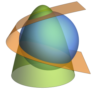
The paraboloid S3 has the symmetry axis parallel to the -axis, and passing through the points , . Its vertex is located at . The advantage of S3 appears when discussing the limit of . Then, the paraboloid does not change the shape and the intersections of S1 and S3 are circles because of coincidence of the symmetry axes. Contrarily to this, setting in S2 results in degeneracy: the cylinder breaks in two parallel planes. On the other hand, turns the paraboloid into a (circular) cylinder, whereas S2 retains its shape. Thus, S2 and S3 (or and ) can be considered complementary, although the regularity at seems to us more favorable (e.g. if some perturbation approach is based upon the small inclination assumption).
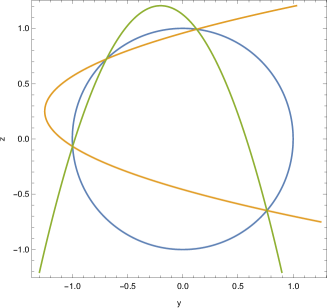
An integral curve can be represented as a parametric curve in a number of ways. Of course, the best is to solve Eqs. (9) and find . But before we accomplish it (and, actually, in order to do it) let us consider parameterizations, where two coordinates are expressed in terms of the third. The most straightforward is to solve the system of S1 and S2 equations, using as a parameter variable, which leads to
| (15) |
All three invariant surfaces S1, S2, S3 intersect the plane , which is their common plane of symmetry. The integral curves, as the lines of intersection of S1, S2, and S3 also pass through and are symmetric with respect to this plane. Moreover, both and coordinates of a given integral curve attain their local extremes at , according to equations of motion (13).
2.3 Intersections with the plane
To find the intersection points of an integral curve with the plane for some specified energy , it is enough to find either or coordinate. Knowing one of them, one might recover the other from the relation . But this involves the ambiguity of sign, thus it is better to find , and then use the parametric equation (15) for . To benefit from minor simplifications, we first find and then .
According to Eq. (15), the relation between and is
| (16) |
where is a polynomial of degree 4
| (17) |
Note the absence of the cubic term thanks to the use of the shifted variable .
Solving the quartic equation is a tedious task; the details can be found in Appendix A. Briefly, the four roots are given in terms of the three roots of the reduced cubic resolvent equation (additionally modified to match the standard cubic polynomial appearing in the Weierstrass elliptic integrals). Depending on the parameters and , selecting some energy value , the number of meridian intersection points is 4, 3, 2, 1, or 0.
Four intersection points mean that there are two distinct integral curves with the same energy, each intersecting in two points:
| (18) |
for a lower curve, and
| (19) |
for the upper curve, with defined in Eq. (141) as functions of , , and , such that .
Three intersection points mean that either one of the two curves contracts to a single point, or two curves share the same intersection point. These situations are distinguished by the sign of invariant from Eq. (135).
-
•
If , then the upper curve shrinks into a point with
(20) The remaining intersection points of the lower curve are
(21) The expressions of and are given in Eq. (145).
-
•
If , then the upper and the lower curves meet at
(22) with the remaining intersection points at
(23)
If , then from Eq. (21) becomes equal to an only two intersection points remain
| (24) |
with . This case requires a unique value of energy with a simple expression (154).
A more generic situation with two intersection points occurs when defines only one trajectory, with given by
| (25) | |||||
where and are defined in Eqs. (142) and (144). Two other roots of , i.e. and are complex, so they do not define the intersections – see Eqs. (151).
Finally, one intersection point means that for the energy there is only one integral curve that contracted to a point with
| (26) |
and given by Eq. (145).
In further discussion, the point of intersection of a regular curve with the plane will be named a turning point, unless it is an equilibrium from the dynamical point of view.
2.4 Cassini states and homoclinic orbits
Finding the Cassini states can be approached from different points of view. Geometrically, they are the points of tangency of the surfaces S1, S2, and S3. Algebraically, they are the multiple roots of , and . Dynamically, they are the fixed points of equations of motion (9) or, equivalently, the local extremes and saddle points of the Hamiltonian on a sphere S1.
In principle, the multiple roots have been found in Section 2.3. But they are given in terms of , which is an implicit function of and as a root of , where is the discriminant of , defined in Eq. (136). Hence, one possible way is to find the roots of , which is a quartic equation in , and substitute them into , , or from Sect. 2.3 (we already did it for ). The alternative is to find the stationary points of the Hamiltonian and use them to evaluate the energy by the substitution into . The latter path is more convenient and was recently taken by Saillenfest et al (2019).
Discussing the Cassini states as the multiple roots of , we should include the information, that they are also the roots of its derivative . Since two polynomials have a common root if and only if their resultant equals zero, we ask about the solutions of . If we treat and as polynomials in , the result is simply the discriminant from Eq. (136), multiplied by a constant (negative) factor. Yet, we can also treat and as polynomials of with degrees 2 and 1, respectively, whose coefficients depend on . So, using
| (27) | |||
| (28) |
we obtain the resultant , where
| (29) |
and
| (30) |
For easier reference to Saillenfest et al (2019), we abandon the shifted variables and solve , which is the same equation as the one they used. However, thanks to considering the Cartesian variables on a sphere, we do not have to warn about any loss of sign, because it does not occur neither in evaluating , nor in obtaining . The value of associated with a given results directly from the condition in Eq. (9), being
| (31) |
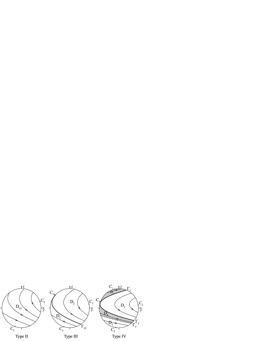
Solving we can recycle the procedure used for . More details can be found in Appendix B, so here we only summarize the final results. When considering the problem on a sphere, there are only two generic situations: either there are two Cassini states and , or there are four of them: , , and . Let us call the former case ‘the Colombo top problem of type II’, and the latter - ‘type IV’. The special case when there are three Cassini states will be called ‘the Colombo top problem of type III’ (see Fig. 2).
In the following subsections we briefly review each type, providing the coordinates of the Cassini states as the functions of and parameters. To avoid confusion with the expressions of Sect. 2.3, we label the coordinates of as , and (of course, for all the points). We only provide that allows to find from Eq. (31) and then the energy of the Cassini state is
| (32) |
Substituting this energy value into an appropriate , , , or from Sect. 2.3, should result in returning to the expression of in terms of and .
2.4.1 Type II
When , the dynamics on a sphere is relatively simple. There are two stable equilibria (elliptic points): at the lower () hemisphere and at the upper hemisphere, located at
| (33) |
where
| (34) |
and, according to Eqs. (164) and (163)
| (35) |
We can identify the Cassini states coordinates as , and , where is given by Eq. (26).
The energy values in the type II problem are bounded by . All trajectories with energy are simple periodic curves (one for each value of ), oscillating in between and , as given by Eqs. (25). Extending and modifying the domains labeling of Henrard and Murigande (1987), let us label the entire sphere surface (with the two Cassini states excluded) as (Fig. 2, left).
2.4.2 Type IV
When , the flow is shaped by the presence of three elliptic fixed points , , , and a hyperbolic point (Fig. 2, right). The latter is accompanied by two homoclinic orbits – upper and lower . Thus the sphere is first partitioned into three domains: between and , between , , , and the third area bounded by and . But the last of the three domains is further divided by the curve whose energy equals that of – the thick dashed curve in Fig. 2. The subdomains and may look similar from the geometrical point of view, but note the fact that each curve in has a companion in with the same energy, which is not the case in .
Equations (171) from Appendix B can be used as they are, but here we add an alternative form, based upon the transformation (129).
| (36) | |||||
where
| (37) |
and
| (38) |
From we infer . The associated coordinates satisfy inequalities .
The energy values are . Referring to Sect. 2.3, we identify , , , and . The unstable equilibrium energy is of special importance, because it serves to determine the turning points of the separatrices from Eq. (23): for , and for .
For the energy values , when , each refers to two periodic curves: one in with the turning points given by (18), and one in with given by Eq. (19). An energy in defines only one periodic trajectory in , and each defines one periodic curve in . Since in both cases, the turning points are given by from Eq. (25).
2.4.3 Type III
The case of is specific, but it has to be included to understand the bifurcation between the two neighboring types. Increasing and/or from the type IV, we observe that the two Cassini states and merge into a single point of neutral stability, the homoclinic orbit contracts to a point, and the separatrix merges with the specific periodic orbit into . Thus the domains and disappear. In course of transition from type III to type II, the division between and disappears, hence we merge them into a single . Lanchares and Elipe (1995) refer to this transition under the name of teardrop bifurcation.
The coordinates of the Cassini states can be obtained from Eq. (174) and are expressible in terms of or alone, resulting in
| (39) |
and
| (40) |
where
| (41) |
The expression of the energy at is so simple, that we write it explicitly
| (42) |
It is useful also in finding the turning point of at , which is
| (43) |
For regular trajectories with , and , their turning points are given by and from Eq. (25), which also means .
3 Analytical solution
3.1 Weierstrass form
3.1.1 General framework
Equations of motion (9) or (13) admit an exact analytical solution in terms of the elliptic functions. Actually, the solution hinges upon the fact that the variable can be considered separately from the remaining two. To see it, we can differentiate , substitute from the first of Eqs. (13), and use the energy integral (11) to eliminate , obtaining
| (44) |
Equation (44) defines a 1 degree of freedom, conservative system with the potential
| (45) |
and the energy integral
| (46) |
But the potential and the energy are closely related to the polynomial :
| (47) |
Thus, whether we use Eq. (46), or the squared Eqs. (13) and (16), the outcome is , amenable to the separation of variables method.
Since is a quartic polynomial, finding amounts to inverting the elliptic integral
| (48) |
where , and the right-hand side evaluates to
| (49) |
The integral to the left of (48) should be a monotonous function of to allow the inversion (solving for ). In the admissible range of between two turning points (or one turning point and an unstable equilibrium) the sign of is constant, which allows to establish its value from the initial condition and to pull out of the integrand.
The integral to the left of Eq. (48) is an elliptic integral and it can be reduced to the Weierstrass normal form by an appropriate transformation , so that
| (50) |
where is the cubic polynomial of the Weierstrass resolvent (133) for , with the invariants , defined in Appendix A.2 – Eqs. (134) and (135). Note that the initial value is always mapped to , regardless of the ordering of the integration limits and , which explains the presence of in the forthcoming transformations.
Solving the rightmost part of Eq. (50) amounts to the substitution of the Weierstrass elliptic function
| (51) |
In all further instances we will use the abbreviated notation for the Weierstrass function , whenever the invariants and from Appendix A.2 are used. Only the invariants different than and will be added to the list of arguments if needed. The derivative od the Weierstrass function obeys
| (52) |
and in the first half-period , we have . Thus, indeed
| (53) |
as expected from Eq. (50).
Once the solution for the first half-period is found, its continuation can be investigated by the substitution into Eq. (44) which is free from the restrictions imposed by the inversion procedure.
3.1.2 Initial conditions at turning point
Let us begin with the easiest situation, when the initial condition is , and is the epoch of crossing the turning point , i.e. . Then the integral to the left of (50) is reduced to the Weierstrass normal form in variable through the rational transformation (Enneper, 1890; Bianchi, 1901)
| (54) |
Replacing the subscript with in the formulae of Sect. 3.1.1, we find
| (55) |
where
| (56) |
Thanks to the symmetry of trajectory with respect to the turning point, the solution does not depend on , and remains valid for all values of .
3.1.3 Arbitrary initial conditions: Weierstrass–Biermann form
If the initial conditions are not at the turning point, i.e. , the transformation is more cumbersome than (54). Whittaker and Watson (1927) quote two alternative forms of the final solution: one due to Weierstrass, published by Biermann (1865), and one by Mordell (1915). Actually, there is yet another, formally elegant form – the secondo metode d’inversione of Bianchi (1901), but the relation of its constants to initial conditions is rather awkward, so we do not consider it here.
The Weierstrass-Biermann form results from the substitution (Enneper, 1890)
| (59) | |||||
| (60) |
where is the sign of , and
| (61) |
are the Taylor coefficients in
| (62) |
After expressing in terms of the initial conditions, they take the form
| (63) |
Substituting , and recalling that over the first half-period, we obtain
| (64) |
Then, accounting for Eqs. (63) and the fact that ,
| (65) |
The substitution into Eq. (44) with the initial condition , shows that the formula (65) is actually valid for all values of , so the initial restriction to the first half-period can be abolished.
Like before, the remaining two variables are found from the energy integral and from the equations of motion, respectively. Thus for we have simply
| (66) |
whereas , requires the differentiation and some manipulations leading to
| (67) |
where the second derivative has been removed using the identity .
3.1.4 Arbitrary initial conditions: Safford form
If , so , the above solution simplifies to Eqs. (58) in a straightforward manner. On the other hand, as pointed out by Safford (1919), the general solution (64) can be derived from the particular solution (55) by assuming , and making use of the addition theorem for the Weierstrass function . Given the initial conditions at , we can find the turning point coordinates for this trajectory using the formulae of Sect. 2.3. Then, according to Safford (1919), the phase is defined through Eq. (60) at , giving . Thus, as an alternative to using Eqs. (65) and (66) for arbitrary initial conditions, one can first compute , and then apply the particular solution (58) with .
But Safford (1919) cared solely about the reduction of the integrand form, so he paid no attention to the problem that is uniquely invertible only in the domain , i.e. within the first half-period. In order to properly place the phase in the full period range , one needs the information about the sign of the derivative . To this end, we take a slightly different approach, that actually leads to a simpler expression for . Substituting , and in Eqs. (58), we can solve them to find
| (68) | |||||
| (69) |
and this set allows the unique determination of the phase. Then, we can apply Eqs. (58) to obtain
| (70) |
with and derived from the energy integral.
Compared to the Weierstrass-Biermann solution, we gain the simplicity at the expense of pre-computing the turning point coordinates and the phase for the given (arbitrary) initial conditions.
3.1.5 Arbitrary initial conditions: Mordell form
The inversion formula of Mordell (1915) was formulated in the language of homogeneous binary forms; in order to apply it to the Colombo top problem, let us translate it to the univariate polynomials framework. The link is simple: the quartic polynomial from Eq. (122), and the quartic binary form
| (71) |
can be matched by
| (72) |
Thus, after the substitution , Eq. (50) is equivalent to
| (73) |
where the definite integral in has been replaced by a path-independent line integral. Skippping the intermediate steps described in (Mordell, 1914, 1915), the inversion of (73) results in
| (74) |
where , and is the Hessian covariant111In this paper we use the Hessian covariant as defined by Janson (2011), which is the same as in Whittaker and Watson (1927). Its sign is opposite to the one originally applied by Mordell (1915). of .
From the correspondence rules (72) we derive
| (75) | |||||
where are defined in Eq. (63). By letting , and , we find that (74) and (75) amount to
| (76) |
Proceeding like in Sect. 3.1.3 we obtain the final form
| (77) |
looking different from the Weierstrass-Biermnann solution (65), yet providing the same values of . Notably, the Mordell solution involves only the first power of .
In order to demonstrate the equivalence of the Weierstrass-Biermann and the Mordell solutions, one can multiply the numerator an the denominator in Eq. (65) by the factor
use the identity , and substitute the expressions of the invariants in terms of
| (78) |
by analogy with the definitions (134) and (135). The result of this procedure is the Mordell solution (77). Obviously, both (65) and (77) admit the same limit expression (58) when and .
As usually, the solution for and can be derived from the equations of motion and the energy integral, like in Sect. 3.1.3.
3.2 Solution in terms of the Jacobi elliptic functions
3.2.1 Weierstrass functions in terms of the Jacobi functions
Although the solution in terms of the Weierstrass function presented in Sect. 3.1 may look universal, its qualitative properties depend on the values of the invariants through the sign of the discriminant . Indeed, the sign plays the central role in expressing the solution in terms of the Jacobian elliptic functions. In this section, only the generic, cases are to be discussed.
The basic relation between the Weierstrass and Jacobi functions is formally universal (Byrd and Friedman, 1971)
| (79) | |||||
| (80) | |||||
where
| (81) |
But if we restrict considerations to the real arguments and moduli of the elliptic functions, the above expressions are valid only if the discriminant from Eq. (136) is positive.
When , which means complex and , the appropriate form is (Abramowitz and Stegun, 1972)
| (82) | |||||
| (83) | |||||
where
| (84) |
The two cases are linked by the complex modulus transformation – see Byrd and Friedman (1971, formula 165.07).
Let the initial conditions at the epoch be . The equations relating the Jacobi and Weierstrass functions can be substituted in to any of the solution forms provided in Sect. 3.1. For the Weierstrass–Biermann or the Mordell form, it is enough to compute the energy and the discriminant to choose the appropriate set (79,80) or (82,83). Then, from the invariants the roots are found, which allows the computation of or for any epoch .
Below, we discuss the Safford form from Sect. 3.1.4, which allows to use the initial conditions at any , but requires the turning point coordinates as supplementary parameters. Having computed two appropriate turning points, such that either , or , we pick one of them as the reference point to be used in Eq. (70). Then, after determining phase with respect to the turning point , the motion can be computed for any epoch , using .
3.2.2 Motion in and
The case occurs only in type IV, when the energy is bounded by : either in the domain , where turning points are given by Eq. (19) with , or in the domain , where the turning points are given by Eq. (18) and . Then, selecting any appropriate as the reference point, we can use the expressions
| (85) | |||||
| (86) | |||||
| (87) |
where
| (88) |
and the phase in
| (89) |
can be computed from the incomplete elliptic function of the first kind F:
| (90) | |||||
| (91) |
The motion is periodic and the period (with respect to time ) is given by the complete elliptic integral of the first kind K
| (92) |
3.2.3 Motion in , and
The common feature of trajectories in domains , and is the negative discriminant . Thus, given the initial conditions and resulting energy, we pick or computed from Eqs. (25) as the reference point and compute, for any
| (93) | |||||
| (94) | |||||
| (95) |
where
| (96) |
The phase in
| (97) |
results from
| (98) | |||||
| (99) |
The related period is
| (100) |
The above formulation is universal, i.e. appropriate in types II, III, and IV, provided .
3.3 Special cases
3.3.1 Reduction rules
By special cases we mean the ones where elliptic functions reduce to the elementary ones. They could be studies by taking limits of the Jacobi functions at or tending to 0 or 1. But it is more direct to observe that each of the special cases, be it the Cassini states, separatrices, or the special curve , results from the reduction of the Weierstrass function to the special case
| (101) |
Since implies , reduction to the above form is always possible by the homogeneity relations (Abramowitz and Stegun, 1972)
| (102) |
except for , when
| (103) |
For the derivative , respective equations are obtained by straightforward differentiation.
Depending on the sign of , two procedures are available. For , the substitution of leads straight to
| (104) |
where , according to Eq. (145).
If , two steps are taken. First, letting , we convert
| (105) |
Then, with , we recover
| (106) |
according to Eq. (146).
3.3.2 Cassini states and
When discussing the Cassini states, we can use the simplest form (58) for . Although the time dependence at the Cassini states does vanish due to , and , it remains of interest to inspect in the numerator, because its period is the period of small oscillations around the stable equilibrium.
Given and , one should first establish the problem type in order to compute the appropriate coordinate , or . These are Eqs. (33), (40), and (36) for the types II, III, and IV, respectively. Starting from this point, the procedure is common: gives the energy of the Cassini state
| (107) |
which substituted in Eq. (134) or (135) gives the invariants or – both positive.
3.3.3 Cassini state and homoclinic orbits ,
The energy of the unstable Cassini state can be evaluated from Eq. (107) with , and given by (36). However, we need it not for the Cassini state itself, but rather to describe the motion on homoclinic orbits having the energy , which are and . To this end, we will use the Safford form (70) with the reference points given by Eq. (23), namely: for , and for .
Since , the reduction (106) leads to
| (109) | |||||
with the coefficients
| (110) |
where is given by Eq. (146). The argument
| (111) |
whose phase with respect to at the initial epoch is given by
| (112) |
Note that the time rate of argument is the same at both the separatrices, and, as expected the solution tends to the Cassini state asymptotically at .
3.3.4 Cassini state and special orbit
The Cassini state , being a stable equilibrium with , is characterized by the period of small oscillations given directly by the formula (108) with the energy evaluated at , deduced from Eq. (36). What makes the difference, compared to or , is the presence of another trajectory having the energy – the special curve .
The motion along can be described using the Safford form solution (70) with respect to the turning points or , given by Eq. (21). Then, performing the reduction (104), we obtain the solution in terms of trigonometric functions
| (113) | |||||
where
| (114) |
The argument is
| (115) |
where , as in Eq. (81) for , hence the time period of the solution is the same as that of small oscillations around , i.e. given by Eq. (108). The phase can be computed from
| (116) |
3.3.5 Cassini state and special orbit
The most degenerate case occurs in type III, where is the cusp (parabolic) equilibrium with energy given by Eq. (42). The homoclinic curve with this energy can be parameterized using rational functions of time, as indicated by the reduction formula (103). For the sake of using the Safford form, we introduce
| (117) |
where is the time interval between the initial epoch and the epoch of crossing the reference turning point with coordinates , and , as given by Eq. (43). Then, with ,
| (118) | |||||
| (119) | |||||
| (120) |
The time offset is given by
| (121) |
4 Conclusions
It is common to describe the integral curves of the Colombo top problem as an intersection of a parabolic cylinder and a unit sphere, the latter being centered at the origin of the coordinate system. We have proposed a new point of view: the curves can be tracked along the intersection of two out of the three invariant surfaces: a parabolic cylinder, a sphere, and a paraboloid of revolution. This thread has been merely signaled, but it can be of possible interest when designing geometric integrators for the numerical treatment of the Colombo top motion. Moreover, using the shifted coordinates , one introduces the symmetry to the parabolic cylinder on the paraboloid (at the expense of having an off-centered sphere) which does simplify a number of expressions given in this work.
When partitioning the phase space of the Colombo top problem, we have completed the landscape, well known from earlier works, with an interesting but hitherto overlooked feature: the trajectory which is unique by being periodic, yet expressible in terms of elementary functions of time. Its presence calls for the distinction of and domains even though qualitatively they look similar. It also adds to a better understanding of the parametric bifurcation associated with the passage from type II, to type IV.
The analytical expressions for the turning points of the Colombo top trajectories as functions of energy, given in Sect. 2.3, had not been reported so far. The expressions for the location of the Cassini states from Sect. 2.4 depend only on parameters . Up to some rearrangement of terms, they are similar to those of Saillenfest et al (2019) in type II or III. For type IV, when , the Cardano form provided by Saillenfest et al (2019) is formally correct, but it gives real values only as the sums of two complex conjugates (casus irreducibilis of the resolvent cubic). In the present work we have preferred to use expressions based on the purely real trigonometric form whenever the quartic has a positive discriminant.
The differential equation for , with its right-hand side proportional to the square root of the degree 4 polynomial, is not a novelty in celestial mechanics. The same form pops up while discussing the Second Fundamental Model of resonance (Henrard and Lemaitre, 1983). Its solution in terms of the Weierstrass elliptic function has always been given either in the simplified form of Eq. (55), as in (Ferraz-Mello, 2007), or in the Biermann-Weierstrass form (Nesvorný and Vokrouhlický, 2016). We have taken an opportunity to recall other possibilities (Safford and Mordell forms) than can be of use in other applications as well.
We hope that the results of the present work will facilitate the study of perturbed Colombo top problems. They should be useful either as the kernel of analytical perturbation procedures, or as a building block of numerical integrators based upon composition methods.
Acknowledgements.
The work of DV was funded by the Czech Science Foundation (grant 18-06083S).Compliance with ethical standards
Conflict of interest The authors S. Breiter, J. Haponiak and D. Vokrouhlický declare that they have no conflict of interest.
The article is partially based upon the doctoral thesis prepared by J. Haponiak, but it includes the results obtained independently by the co-authors.
References
- Abramowitz and Stegun (1972) Abramowitz M, Stegun IA (1972) Handbook of Mathematical Functions, Applied Mathematics Series, vol 55. National Bureau of Standards, Washington DC
- Atobe and Ida (2007) Atobe K, Ida S (2007) Obliquity evolution of extrasolar terrestrial planets. Icarus 188(1):1–17, DOI 10.1016/j.icarus.2006.11.022, arXiv:astrop-ph/0611669
- Atobe et al (2004) Atobe K, Ida S, Ito T (2004) Obliquity variations of terrestrial planets in habitable zones. Icarus 168(2):223–236, DOI 10.1016/j.icarus.2003.11.017
- Bianchi (1901) Bianchi L (1901) Lezzioni Sulla Teoria delle Funzioni di Variabile Complessa e delle Funzioni Ellittiche. Enrico Spoerri, Pisa
- Biermann (1865) Biermann WGA (1865) Problemata Quaedam Mechanica Functionum Ellipticarum Ope Soluta. Carl Schulze, Berlin
- Boué et al (2009) Boué G, Laskar J, Kuchynka P (2009) Speed limit on Neptune migration imposed by Saturn tilting. Astrophys J Lett 702(1):L19–L22, DOI 10.1088/0004-637X/702/1/L19, arXiv:astrop-ph/0909.0332
- Brasser and Lee (2015) Brasser R, Lee MH (2015) Tilting Saturn without tilting Jupiter: constraints on giant planet migration. Astron J 150(5):157, DOI 10.1088/0004-6256/150/5/157, arXiv:astrop-ph/1509.06834
- Brizard (2015) Brizard AJ (2015) Notes on the Weierstrass Elliptic Function. arXiv e-prints arXiv:math-ph/1510.07818
- Byrd and Friedman (1971) Byrd PF, Friedman MD (1971) Handbook of Elliptic Integrals for Engineers and Scientists. Springer-Verlag, Berlin, Heidelberg, New York
- Cassini (1693) Cassini GD (1693) De l’origine et du progrés de l’Astronomie, et de son usage dans la Geographie et dans la Navigation. In: Recueil d’observations faites en plusieurs voyages par ordre de Sa Majesté pour perfectionner l’astronomie et la geographie, l’Imprimerie Royale, Paris, pp 1–43
- Colombo (1966) Colombo G (1966) Cassini’s second and third laws. Astron J 71:891–896, DOI 10.1086/109983
- Copernicus (1543) Copernicus N (1543) De Revolutionibus Orbium Coelestium. Johannes Petreius, Nuremberg
- Correia and Laskar (2001) Correia ACM, Laskar J (2001) The four final rotation states of Venus. Nature 411(6839):767–770, DOI 10.1038/35081000
- Efimov et al (2018) Efimov S, Pritykin D, Sidorenko V (2018) Long-term attitude dynamics of space debris in Sun-synchronous orbits: Cassini cycles and chaotic stabilization. Celest Mech Dyn Astron 130(10):62, DOI 10.1007/s10569-018-9854-4, arXiv:physics.space-ph/1712.08596
- Enneper (1890) Enneper A (1890) Elliptische Functionen. Theorie und Geschichte. Verlag von Luis Nebert, Halle
- Ferraz-Mello (2007) Ferraz-Mello S (2007) Canonical Perturbation Theories – Degenerate Systems and Resonance. Springer, New York, DOI 10.1007/978-0-387-38905-9
- Hamilton and Ward (2004) Hamilton DP, Ward WR (2004) Tilting Saturn. II. Numerical model. Astron J 128(5):2510–2517, DOI 10.1086/424534
- Harris and Ward (1982) Harris AW, Ward WR (1982) Dynamical constraints on the formation and evolution of planetary bodies. Ann Rev Earth Planet Sci 10:61, DOI 10.1146/annurev.ea.10.050182.000425
- Henrard (1993) Henrard J (1993) Dynamics Reported, vol 2, Springer, Berlin, Heidelberg, chap The Adiabatic Invariant in Classical Mechanics, pp 117–235. DOI 10.1007/978-3-642-61232-9_4
- Henrard and Lemaitre (1983) Henrard J, Lemaitre A (1983) A Second Fundamental Model for resonance. Celest Mech 30(2):197–218, DOI 10.1007/BF01234306
- Henrard and Murigande (1987) Henrard J, Murigande C (1987) Colombo’s top. Celest Mech 40:345–366, DOI 10.1007/BF01235852
- Janson (2011) Janson S (2011) Invariants of polynomials and binary forms. arXiv e-prints math.HO/1102.3568
- Lagrange (1764) Lagrange JL (1764) Recherches sur la libration de la Lune. Prix de l’Academie Royale des Sciences de Paris IX:1–50
- Lagrange (1780) Lagrange JL (1780) Théorie de la libration de la Lune. Nouveau Mémoires de l’Academie Royale des Sciences et Belles-Lettres de Berlin (unnumbered):203–308
- Lanchares and Elipe (1995) Lanchares V, Elipe A (1995) Bifurcations in biparametric quadratic potentials. Chaos 5(2):367–373, DOI 10.1063/1.166107
- Laskar and Robutel (1993) Laskar J, Robutel P (1993) The chaotic obliquity of the planets. Nature 361(6413):608–612, DOI 10.1038/361608a0
- Laskar et al (1993) Laskar J, Joutel F, Robutel P (1993) Stabilization of the Earth’s obliquity by the Moon. Nature 361(6413):615–617, DOI 10.1038/361615a0
- Mordell (1914) Mordell LJ (1914) Indeterminate equations of the third and fourth degrees. Quart J Pure Appl Math 45:170–186
- Mordell (1915) Mordell LJ (1915) The inversion of the integral (…). Messenger of Mathematics 44:138–141
- Nesvorný and Vokrouhlický (2016) Nesvorný D, Vokrouhlický D (2016) Dynamics and transit variations of resonant exoplanets. Astrophys J 823(2):72, DOI 10.3847/0004-637X/823/2/72, arXiv:astro-ph/1603.07306
- Neumark (1965) Neumark S (1965) Solution of Cubic and Quartic Equations. Pergamon Press, Oxford
- Peale (1974) Peale SJ (1974) Possible histories of the obliquity of Mercury. Astron J 79:722, DOI 10.1086/111604
- Rogoszinski and Hamilton (2020) Rogoszinski Z, Hamilton DP (2020) Tilting ice giants with a spin-orbit resonance. Astrophys J 888(2):60, DOI 10.3847/1538-4357/ab5d35, arXiv:astro-ph/1908.10969
- Safford (1919) Safford FH (1919) Reduction of the elliptic element to the Weierstrass form. Bull Am Math Soc 26(1):13–16
- Saillenfest et al (2019) Saillenfest M, Laskar J, Boué G (2019) Secular spin-axis dynamics of exoplanets. Astron Astroph 623:A4, DOI 10.1051/0004-6361/201834344, arXiv:astro-ph/1901.02831
- Tisserand (1891) Tisserand F (1891) Traité de Mécanique Céleste, vol 2. Gauthier-Villars, Paris
- Vokrouhlický and Nesvorný (2015) Vokrouhlický D, Nesvorný D (2015) Tilting Jupiter (a bit) and Saturn (a lot) during Planetary Migration. Astrophys J 806(1):143, DOI 10.1088/0004-637X/806/1/143, arXiv:astro-ph/1505.02938
- Vokrouhlický et al (2003) Vokrouhlický D, Nesvorný D, Bottke WF (2003) The vector alignments of asteroid spins by thermal torques. Nature 425(6954):147–151, DOI 10.1038/nature01948
- Vokrouhlický et al (2006) Vokrouhlický D, Nesvorný D, Bottke WF (2006) Secular spin dynamics of inner main-belt asteroids. Icarus 184(1):1–28, DOI 10.1016/j.icarus.2006.04.007
- Ward (1973) Ward WR (1973) Large-scale variations in the obliquity of Mars. Science 181(4096):260–262, DOI 10.1126/science.181.4096.260
- Ward (1974) Ward WR (1974) Climatic variations on Mars: 1. Astronomical theory of insolation. J Geophys Res 79(24):3375–3386, DOI 10.1029/JC079i024p03375
- Ward (1975) Ward WR (1975) Past orientation of the Lunar spin axis. Science 189(4200):377–379, DOI 10.1126/science.189.4200.377
- Ward (1982) Ward WR (1982) Comments on the long-term stability of the Earth’s obliquity. Icarus 50(2-3):444–448, DOI 10.1016/0019-1035(82)90134-8
- Ward and Canup (2006) Ward WR, Canup RM (2006) The obliquity of Jupiter. Astrophys J Lett 640(1):L91–L94, DOI 10.1086/503156
- Ward and de Campli (1979) Ward WR, de Campli WM (1979) Comments on the Venus rotation pole. Astrophys J Lett 230:L117–L121, DOI 10.1086/182974
- Ward and Hamilton (2004) Ward WR, Hamilton DP (2004) Tilting Saturn. I. Analytic model. Astron J 128(5):2501–2509, DOI 10.1086/424533
- Whittaker and Watson (1927) Whittaker ET, Watson GN (1927) A Course of Modern Analysis, 4th edn. Cambridge University Press, Cambridge
Appendix A The roots of
A.1 Factorization
In order to find the zeroes of the , let us first write it in the ‘classical’ polynomial form
| (122) |
where, according to Eq. (17) the coefficients are
| (123) |
Note the absence of the cubic term (), meaning that equation is already in the reduced form.
Solving equation , we essentially follow a simplified and slightly reformulated procedure of Neumark (1965). In particular, the absence of the third power of allows the factorization
| (124) |
with only three parameters (, , ), and three conditions resulting from equating the coefficients of and :
| (125) |
The last two equations are easily solved for and
| (126) |
so the first of Eqs. (125), after the substitution of Eq. (126), is actually the resolvent cubic equation
| (127) |
where , according to Eq. (30). The Descartes rule guarantees that (for nonzero and ) the resolvent has at least one positive real root to be used in factorization (124).
Before we proceed to solving the resolvent, let us make some important remarks. The four roots of the quartic equation come in two pairs of the roots of and , i.e.
| (128) |
Let be the only, or the greatest positive root of the resolvent (127). Then, from the Vieta’s formulas, we find for the remaining two roots , and , which allows to see that
| (129) |
This leads to the Euler form of the solution
| (130) |
Assuming for the real roots , we guarantee a number of properties like the ordering , the fact that a given trajectory contains only a pair or , and that if are complex conjugates, then and remain real, whereas and become complex.
A.2 Weierstrass resolvent and its roots
The cubic resolvent equation (127) can be brought to a reduced form without the square term in a number of ways. We choose the substitution based upon the seminvariant (Janson, 2011)
| (131) |
with
| (132) |
Applying it to Eq. (127), and multiplying both sides by 4, we obtain
| (133) |
The cubic polynomial plays a special role in the theory of the Weierstrass elliptic functions, thus let us call it the Weierstrass resolvent. The symbols and that appear in Eq. (133) are the two, algebraically independent, basis invariants of the quartic :
-
•
the apolar invariant of degree 2
(134) - •
Notably, both the discriminants: of the quartic , and of the cubic are not only expressible in terms of and , but they are equal up to a constant factor. If
| (136) |
then .
Let the roots of the Weierstrass resolvent equation be , , and . By the Vieta’s formulae, they satisfy
| (137) |
and by the definition of the scaled discriminant (136)
| (138) |
Introducing auxiliary quantities and , such that
| (139) |
hence
| (140) |
we can establish the universal formula for the roots (Brizard, 2015)
| (141) | |||||
If (hence ) there are three simple real roots given directly by Eqs. (141). When , there is one real root and two complex ones, with . Equations (139) and (141) remain valid in principle, but they involve complex quantities and require distinguishing the sign of . In these circumstances it is more convenient to use the Cardano form for the real root222In this approach, of a real argument is used as a real-valued function for , i.e. .
| (142) |
and
| (143) |
with
| (144) |
for the complex roots.
Finally, the degeneracy implies real roots: one simple and one double, or one triple root. The former case requires and ; then, according to the sign of , either
| (145) |
or
| (146) |
The ordering of roots in (146) is exceptional ( is the greatest), but helps to maintain a coherent notation in further applications.
The triple root may appear only for , which is possible only when .
A.3 The roots
Although the roots of are to be expressed in terms of the roots of , we need to include in the discussion not only the invariants , , and , but also seminvariants and
| (147) |
This is due to the fact that although formally it is enough to substitute
| (148) |
into (130), the signs of play a significant role in determining which of the roots are real and which are complex, and there are various ways to create multiple roots.
In the following discussion we will refer to the Theorem 9.3 of Janson (2011), adjusted to the different scaling of our invariants and seminvariant (namely, his , , , and ).
A.3.1 Four simple real roots ( and all )
If the four real roots exist, they take the form (130) with defined in Eq. (148) and as in (141). This requires not only to have three simple real roots , but also that for each . The latter is secured by and (Janson, 2011). Substituting (131), (134) and (123), we obtain
| (149) |
as the condition for the real quadruple . If is positive, but the second condition in (149) is not fulfilled, there are no real roots, and form two distinct pairs of complex conjugate numbers.
A.3.2 Two simple real roots ()
When and are complex, the pair is complex, whereas in the formula (130) formally remain real-valued, yet only by canceling the imaginary parts. Using , with given by Eq. (142), we can obtain and directly from Eqs. (128) and (126). Alternatively, we can find the expressions for , which results in
| (150) |
and
| (151) |
where
| (152) |
with given by Eq. (142).
A.3.3 Multiple roots ()
The statement means only that at least one of the roots is at least a double root. Further distinction is based upon the signs and values of , and . Let us inspect five possibilities involving multiple real roots from the Theorem 9.3 of Janson (2011).
A quadruple real root is not possible, because it requires , whereas substituting we obtain . Two real double roots are also impossible, because they require (among other conditions) that , which is not the case. The remaining three cases are the following.
-
1.
A triple real root and one single real root appear when , and . Taking the resultant of and considered as the polynomials in , one finds that both the invariants admit the common root if
(153) the relation well known from Henrard and Murigande (1987). With this constraint, can be solved to give a unique negative root
(154) According to the statement below Eq. (146), refers to the triple root , hence, with , we obtain
(155) where is the single, and is the triple root.
- 2.
- 3.
Appendix B Cassini states coordinates
The left-hand side of the quartic equation is the polynomial
| (161) |
where
| (162) |
Evaluating the invariants and seminvariants from the primed coefficients, we find
| (163) |
ant the scaled discriminant is
| (164) |
The transformation
| (165) |
converts the equation into , which is free of the term, and so is ready for the factorization from Sect. A.1. Fortunately, we do not need to know the coefficients of the equation in , because we require only the invariants (163) which are conserved under the simple transformation (165). Thus, tracing backward the procedure from Appendix A, we start with solving the Weierstrass resolvent
| (166) |
finding the roots , , and . These define
| (167) |
as in Eqs. (132) and (148). Finally, four roots are given by Eq. (130) with , and then . Each real solution is the coordinate of some Cassini state.
The number of real roots of depends on the sign of .
- 1.
-
2.
means . The Weierstrass resolvent has one real root and two complex roots given by Eqs. (142), (143), and (144) with , , and . Accordingly, we obtain two real roots – the ones involving , where the imaginary part cancels out. Adapting the expressions (150) and (152), and adjusting the subscripts of to the Cassini states and , we obtain two real roots of as
(172) with . The final substitution is made in Sect. 2.4.
-
3.
, hence , implies one single and one double real root of the Weierstrass resolvent. A triple root is excluded, because . Thus, observing that , and ,
(173) provide three Cassini states: two usual , , and one degenerate , with
(174) listed in the ascending order.