Numerical analysis on boundary integral equation to exterior Dirichlet problem of Laplace equation

Abstract

This paper investigate on numerical analysis on modified Single-layer approach to exterior Dirichlet problem of Laplace equation. We complete the convergence and error analysis of Petrov-Galerkin and Galerkin-Collocation methods with trigonometric basis for the induced modified Symm’s integral equation of the first kind on analytic boundary. Besides, utilizing the composite trapezial quadrature formula and trigonometric interpolation to handle the singularity in modified logarithmic kernel, we establish the numerical procedure for implementation. On these numerical examples, we compare the effect and efficiency of different Petrov-Galerkin and Galerkin-Collocation methods.

• August 2017

1 Introduction

Integral equation method plays an important role in solving the (BVP) of Laplace equations. Let $\Omega\subseteq\mathrm{R}^{2}$ be bounded and simply connected with boundary $\partial\Omega$ of class $C^{2}$ and $f\in C(\partial\Omega)$. To solve Dirichlet problem of Laplace equation

$$\Delta u=0\ \textrm{in}\ \Omega,\ u=f\ \textrm{on}\ \partial\Omega,$$

When $f\in C^{1,\alpha}(\partial\Omega)$, the solution $u$ can be represented as single-layer potential

$$u(x):=-\frac{1}{2\pi}\int_{\partial\Omega}\psi(y)\ln|x-y|ds(y),\quad x\in\mathrm{R}^{2},$$

provided that the density $\psi\in C^{0,\alpha}(\partial\Omega)$ solves

$$S\psi:=-\frac{1}{2\pi}\int_{\partial\Omega}\psi(y)\ln|x-y|ds(y)=f(x),\quad x\in\partial\Omega,$$ (1.1)

(1.1) is known as Symm’s integral equation of the first kind. There exists numerous work on numerical solution of (SIE). Frequently used method is Petrov-Galerkin and collocation methods, for example, Galerkin and collocation boundary element method, see [1,2,3,4,9,10]; Cheybshev polynomial-based collocation method see [17,19]; spline Galerkin and collocation method, see [5,7,8,20,22]; piecewise constant collocation and Galerkin methods, see [8,12,18,21]; wavelet-based or trigonometric-based Galerkin method, see [13, Chapter 3.3] and [11].
For the simplicity and completeness of analysis, we are interested in the numerical analysis of projection methods under Fourier basis for planar (SIE), such as Petrov-Galerkin methods and Galerkin-Collocation method. In past, assuming $\partial\Omega$ to be analytic with nonzero pointwise tangent, that is, $\partial\Omega$ possesses the analytic parameterizations

$$\partial\Omega:=\{\gamma(t):t\in[0,2\pi)\}$$ (1.2)

and $|\gamma^{\prime}(t)|>0,\ t\in[0,2\pi)$. Inserting (1.2) into (1.1), (SIE) is transformed into integral equation of $1$ D:

$$-\frac{1}{2\pi}\int^{2\pi}_{0}\Psi(s)\ln|\bm{\gamma}(t)-\bm{\gamma}(s)|ds=g(t),\quad x\in[0,2\pi],$$ (1.3)

for the transformed density $\Psi(s):=\psi(\bm{\gamma}(s))|\dot{\bm{\gamma}}(s)|$ and $g(t):=f(\bm{\gamma}(t)),\ s\in[0,2\pi]$. Complete convergence and error are obtained (See [13] and references therein) for Petrov-Galerkin methods and Galerkin-Collocation method to $g\in H^{r}(0,2\pi),r\geq 1$ under $L^{2}$ setting.

Similar to interior Dirichlet problem, to solve exterior problem

$$\Delta u=0\quad\textrm{in}\ \mathrm{R}^{2}\setminus\overline{\Omega},\quad u=f\quad\textrm{on}\ \partial\Omega,$$

$$\quad u(x)=u_{\infty}+o(\frac{1}{|x|}),\quad\textrm{for}\ |x|\to\infty.$$

When $f\in C^{1,\alpha}(\partial\Omega)$, with introduction of mean value operator $M$ defined by

$$M:\varphi\mapsto\frac{1}{|\partial\Omega|}\int_{\partial\Omega}\varphi ds,$$

the solution $u$ can be represented as the modified single-layer potential

$$u(x):=-\frac{1}{2\pi}\int_{\partial\Omega}(\varphi(y)-M\varphi)\ln|x-y|ds(y)+M\varphi,\quad x\in\mathrm{R}^{2},$$

provided that the density $\varphi\in C^{0,\alpha}(\partial\Omega)$ solves the integral equation

$$S_{0}\varphi:=-\frac{1}{2\pi}\int_{\partial\Omega}(\varphi(y)-M\varphi)\ln|x-y|ds(y)+M\varphi=f(x),\quad x\in\partial\Omega,$$ (1.4)

Notice that $S_{0}$ is injective on $C(\partial\Omega)$ even with no specific geometric condition on boundary $\partial\Omega$, that is, any $\varphi\in C(\partial\Omega)$ that solves $S_{0}\varphi=0$ can only be trivial (see [15, Theorem 7.41]). Rewrite (1.4) as

$$S_{0}\varphi=\int_{\partial\Omega}G(x,y)\varphi(y)ds(y)$$ (1.5)

where

$$G(x,y):=-\frac{1}{2\pi}\ln|x-y|+\frac{1}{2\pi}\frac{1}{|\partial\Omega|}\int_{\partial\Omega}\ln|x-z|ds(z)+\frac{1}{|\partial\Omega|}.$$ (1.6)

In the following, utilizing the technique in (SIE), we transform the modified Symm’s integral equation into one-dimensional form. Now the regular parameterization

$$\partial\Omega:=\{\gamma(t):t\in[0,2\pi)\}$$

is twice continuously differentiable with $|\dot{\gamma}(t)|>0,\ \forall t\in[0,2\pi]$. Inserting it into (1.5), the modified (SIE) takes the form

$$S_{0}\varphi:=\int^{2\pi}_{0}G(t,s)\Psi(s)ds=g(t),\quad t\in[0,2\pi)$$ (1.7)

with the transformed kernel

$$G(t,s):=$$

$$-\frac{1}{2\pi}\ln|\gamma(t)-\gamma(s)|+\frac{1}{2\pi}\frac{1}{|\partial\Omega|}\int^{2\pi}_{0}\ln|\gamma(t)-\gamma(\sigma)||\gamma^{\prime}(\sigma)|d\sigma+\frac{1}{|\partial\Omega|},$$

the transformed density $\Psi(s):=\varphi(\gamma(s))|{\gamma^{\prime}}(s)|$ and $g(t):=f(\gamma(t)),\ s\in[0,2\pi]$.
The research on numerical analysis of modified Symm’s integral equation for exterior problem of Laplace equation is few. It is indicated in [15, Example 13.23] that, for ellipse boundary curve, the (1.7) can be rewriten as

$$\frac{1}{2\pi}\int^{2\pi}_{0}E(t,\tau)\Psi(\tau)d\tau=g(t),\quad t\in[0,2\pi]$$ (1.8)

where

$$E(t,\tau)=(\ln(4\sin^{2}\frac{t-s}{2})-2)+(\ln(4\sin^{2}\frac{t-s}{2}))K(t,\tau)+L(t,\tau)$$

and $K$, $L$ is infinitely differentiable and $2\pi$ periodic with respect to both variables such that $K(t,t)=0$ for all $0\leq t\leq 2\pi$. Then, the (1.8) can be well handled by Galerkin-Collocation and Petrov-Galerkin methods on trigonometric basis. Besides, there exist some work using modified boundary integral equation with Nyström method to handle exterior Neumann and Robin problem of Laplace equation (See [16,21]). In this paper, we use Lemma 2.4 to determine that all (1.7) on analytic boundary curves can be transformed into form (1.8), and thus, we can extend the convergence and error analysis of Petrov-Galerkin, Galerkin-Collocation methods with trigonometric basis to the more general case.

As to the arrangement of the rest contents. In section 2, we introduce necessary preliminaries, such as periodic Sobolev space, basic properties of modified Symm’s integral operator. In section 3, we analyze the convergence for three Petrov-Galerkin methods and Galerkin-Collocation method respectively. In section 4, we illustrate the numerical procedures and complete the numerical experiments, show the validness of convergence analysis. In section 5, we conclude the whole work of this paper.

2 Preliminaries

2.1 Periodic Sobolev space $H^{r}(0,2\pi)$, trace space $H^{k}(\Gamma)$ and estimates

Throughout this paper, we denote the $2\pi$ periodic Sobolev space of order $r\in\mathrm{R}$ by $H^{r}(0,2\pi)$ (refer to [13,15]). Notice that, for $r>s$, the Sobolev space $H^{r}(0,2\pi)$ is a dense subspace of $H^{s}(0,2\pi)$. The inclusion operator from $H^{r}(0,2\pi)$ into $H^{s}(0,2\pi)$ is compact.
Let $\Gamma$ be the boundary of a simply connected bounded domain $D\subseteq\mathrm{R}^{2}$ of class $C^{k},k\in\mathrm{N}$. With the aid of a regular and $k$ times continuously differentiable $2\pi$ periodic paramater representation

$$\Gamma=\{z(t):t\in[0,2\pi)\}$$

for $0\leq p\leq k$ we can define the trace space $H^{p}(\Gamma)$ as the space of all functions $\varphi\in L^{2}(\Gamma)$ with the property that $\varphi\circ z\in H^{p}(0,2\pi)$. By $\varphi\circ z$, we denote the $2\pi$ periodic function given by $(\varphi\circ z)(t):=\varphi(z(t)),t\in\mathrm{R}$. The scalar product and norm on $H^{p}(\Gamma)$ are defined through the scalar product on $H^{p}(0,2\pi)$ by

$$(\varphi,\psi)_{H^{p}(\Gamma)}:=(\varphi\circ z,\psi\circ z)_{H^{p}(0,2\pi)}.$$

Lemma 2.1

Let $P_{n}:L^{2}(0,2\pi)\longrightarrow X_{n}\subset L^{2}(0,2\pi)$ be an orthogonal projection operator, where $X_{n}=span\{e^{ikt}\}^{n}_{k=-n}$. Then $P_{n}$ is given as follows

$$(P_{n}x)(t)=\sum^{n}_{k=-n}a_{k}e^{ikt},\quad x\in L^{2}(0,2\pi),$$

where

$$a_{k}=\frac{1}{2\pi}\int^{2\pi}_{0}x(s)\exp(-iks)ds,\quad k\in\mathrm{N},$$

are the Fourier coefficients of $x$. Furthermore, the following estimate holds:

$$\|x-P_{n}x\|_{H^{s}}\leq\frac{1}{n^{r-s}}\|x\|_{H^{r}}\quad x\in\ H^{r}(0,2\pi),$$

where $r\geq s$.

Proof 1

See [13, Theorem A.43].

Lemma 2.2

(Inverse inequality): Let $r\geq s$. Then there exists a $c>0$ such that

$$\|\psi_{n}\|_{H^{r}}\leq cn^{r-s}\|\psi_{n}\|_{H^{s}},\quad\forall\ \psi_{n}\in X_{n}$$

for all $n\in\mathrm{N}$.

Proof 2

See [13, Theorem 3.19].

2.2 Integral operator and regularity

Lemma 2.3

Let $r\in\mathrm{N}$ and $k\in C^{r}([0,2\pi]\times[0,2\pi])$ be $2\pi-$ periodic with respect to both variables. Then the integral operator $K$, defined by

$$(Kx)(t):=\int^{2\pi}_{0}k(t,s)x(s)ds,\quad t\in(0,2\pi),$$

can be extended to a bounded operator from $H^{p}(0,2\pi)$ into $H^{r}(0,2\pi)$ for every $-r\leq p\leq r$.

Proof 3

See [13, Theorem A.45].

Lemma 2.4

Let $\partial\Omega$ be the boundary of bounded simply connected domain $\Omega\subseteq\mathrm{R}^{2}$. If $\partial\Omega$ is of class $C^{m+1,\alpha}$ and $\varphi$ of $C^{m,\alpha}$ with $m\in\mathrm{N}$ and $0<\alpha<1$, then the interior single layer potential defined by $\varphi$, that is,

$$\Psi(x):=\int_{\partial\Omega}\varphi(y)\ln|x-y|ds(y),\quad x\in\overline{\Omega},$$

is of class $C^{m+1,\alpha}$ on $\overline{\Omega}$.

Proof 4

See [6, Page 303]

2.3 Modified Symm’s integral equation of the first kind

Throughout this paper, we denote the modified Symm’s integral operator in (1.7) by $S_{0}$.

$$(S_{0}\Psi)(t):=\int^{2\pi}_{0}G(t,s)\Psi(s)ds=g(t),t\in[0,2\pi)$$ (2.1)

with the transformed kernel

$$G(t,s):=$$

$$-\frac{1}{2\pi}\ln|\gamma(t)-\gamma(s)|+\frac{1}{2\pi}\frac{1}{|\partial\Omega|}\int^{2\pi}_{0}\ln|\gamma(t)-\gamma(\sigma)||\gamma^{\prime}(\sigma)|d\sigma+\frac{1}{|\partial\Omega|}.$$

Utilizing the common decomposition technique on kernel (see [13, Chapter 3.3]) in Symm’s integral equation of the first kind, we split kernel $G(t,s)$ into three parts:

$$G(t,s)=G_{1}(t,s)+G_{2}(t,s)+G_{3}(t),$$ (2.2)

where

$$G_{1}(t,s):=-\frac{1}{4\pi}(\ln(4\sin^{2}\frac{t-s}{2})-1)\quad(t\neq s)$$ (2.3)

$$G_{2}(t,s):=-\frac{1}{2\pi}\ln|\gamma(t)-\gamma(s)|+\frac{1}{4\pi}(\ln(4\sin^{2}\frac{t-s}{2})-1)\quad(t\neq s)$$ (2.4)

$$G_{3}(t):=\frac{1}{2\pi}\frac{1}{|\partial\Omega|}\int^{2\pi}_{0}\ln|\gamma(t)-\gamma(\sigma)||\gamma^{\prime}(\sigma)|d\sigma+\frac{1}{|\partial\Omega|}.$$ (2.5)

We note that the logarithmic singularities at $t=s$ in $G(t,s)$ is separated to $G_{1}$, and $G_{1}$ corresponds to the regular representation of disc with center $0$ and radius $a=e^{-\frac{1}{2}}$, that is,

$$\gamma_{a}(s)=e^{-\frac{1}{2}}(\cos s,\sin s),\ s\in[0,2\pi).$$

The second part $G_{2}$ has a analytic continuation onto $[0,2\pi]\times[0,2\pi]$ (See [13, Page 84]) since $\gamma$ is analytic. The third part

$$G_{3}(t)=-\frac{1}{|\partial\Omega|}h(t)+\frac{1}{|\partial\Omega|},\quad t\in[0,2\pi],$$

where

$$h(t)=-\frac{1}{2\pi}\int^{2\pi}_{0}\ln|\gamma(t)-\gamma(\sigma)||\gamma^{\prime}(\sigma)|d\sigma$$

is the single layer potential of constant function $1$ on $\partial\Omega$ which is analytic. By Lemma 2.4, $G_{3}(t)\in C^{\infty}[0,2\pi]$
Now we define integral operators respectively as

$$(S_{1}\Psi)(t):=\int^{2\pi}_{0}G_{1}(t,s)\Psi(s)ds$$ (2.6)

$$(S_{2}\Psi)(t):=\int^{2\pi}_{0}(G_{2}(t,s)+G_{3}(t))\Psi(s)ds.$$ (2.7)

$$(K_{2}\Psi)(t):=\int^{2\pi}_{0}(G_{2}(t,s)+G_{3}(s))\Psi(s)ds.$$ (2.8)

$$(K\Psi)(t):=\int^{2\pi}_{0}(G_{1}(t,s)+G_{2}(t,s)+G_{3}(s))\Psi(s)ds.$$ (2.9)

$$S_{0}=S_{1}+S_{2},\quad K=S_{1}+K_{2}.$$ (2.10)

Lemma 2.5

It holds that

$$\frac{1}{2\pi}\int^{2\pi}_{0}e^{ins}\ln(4\sin^{2}\frac{s}{2})ds=\left\{\begin{array}[]{rcl}-\frac{1}{|n|},&&{n\in\mathrm{Z},n\neq 0},\\ 0,&&{n=0}.\end{array}\right.$$

This gives that the functions

$$\hat{\psi}_{n}(t):=e^{int},\quad t\in[0,2\pi],\ n\in\mathrm{Z},$$

are eigenfunctions of $S_{1}$:

$$S_{1}\hat{\psi}_{n}=\frac{1}{2|n|}\hat{\psi}_{n}\quad\textrm{for}\ n\neq 0\ \textrm{and}$$

$$S_{1}\hat{\psi}_{0}=\frac{1}{2}\hat{\psi}_{0}.$$

Proof 5

See [13, Theorem 3.17]

Lemma 2.6

Let $\Omega\subseteq\mathrm{R}^{2}$ be a simply connected bounded domain with $\partial\Omega$ be its boundary analytic. Then
(a) $S_{0}$ is compact in $L^{2}(0,2\pi)$ and $K=S^{*}_{0}$ when we see $K,S_{0}$ both as operator on $L^{2}(0,2\pi)$.
(b) The operator $S_{1}$ is bounded injective from $H^{s-1}(0,2\pi)$ onto $H^{s}(0,2\pi)$ with bounded inverses for every $s\in\mathrm{R}$, the same assertion also holds for $S_{0},K$.
(c) The operator $S_{1}$ is coercive from $H^{-\frac{1}{2}}(0,2\pi)$ into $H^{\frac{1}{2}}(0,2\pi)$.
(d) The operator $S_{2},K_{2}$ is compact from $H^{s-1}(0,2\pi)$ into $H^{s}(0,2\pi)$ for every $s\in\mathrm{R}$.

Proof 6

See [13, Theorem A.33, Theorem 3.18] for (a),(c) and the former part of (b).
Following the main idea in [13, theorem 3.18], we prove (d) and the latter part of (b). Since the $G_{2}(t,s)+G_{3}(t,s)$ has a $C^{\infty}$ continuation on $[0,2\pi]\times[0,2\pi]$, by Lemma 2.3, $S_{2}$ defines a bounded operator from $H^{s-1}(0,2\pi)$ to $H^{p}(0,2\pi)$ with $s<p$. Composing with compact embedding $H^{p}(0,2\pi)\subset\subset H^{s}(0,2\pi)$, (d) follows.
For the latter part of (b), we see $S_{0}=S_{1}(I+S^{-1}_{1}S_{2})$ and $K=S_{1}(I+S^{-1}_{1}K_{2})$. Notice that, for $s\in\mathrm{R}$, by (d) and former part of (b), $S^{-1}_{1}S_{2}$ and $S^{-1}_{1}K_{2}$ are all compact operators on $H^{s-1}(0,2\pi)$. Now by Riesz theorem (See [13, Theorem A.34 (b)]), if we prove that $(I+S^{-1}_{1}S_{2})$ and $(I+S^{-1}_{1}K_{2})$ are all injective on $H^{s-1}(0,2\pi)$, that is, $S_{0}$ and $K$ are all injective from $H^{s-1}(0,2\pi)$ to $H^{s}(0,2\pi)$, then we prove that $(I+S^{-1}_{1}S_{2})$ and $(I+S^{-1}_{1}K_{2})$ are all surjective on $H^{s-1}(0,2\pi)$ with bounded inverses, that is, $S_{0}$ and $K$ are all surjective from $H^{s-1}(0,2\pi)$ to $H^{s}(0,2\pi)$ with bounded inverses.
Now it is sufficient to prove the injectivity of $S_{0},K$ from $H^{s-1}(0,2\pi)$ to $H^{s}(0,2\pi)$ with $s\in\mathrm{R}$. Let $\Psi\in H^{s-1}(0,2\pi)$ with $S_{0}\Psi=0$. From $S_{1}\Psi=-S_{2}\Psi$ and the mapping properties (Lemma 2.3) of $S_{2}$, we know $S_{1}\Psi\in H^{p}(0,2\pi),\forall p\in\mathrm{R}$ and thus, $\Psi\in H^{1}(0,2\pi)$. This implies that $\Psi$ is continuous and the transformed function $\varphi(\gamma(t))=\frac{\Psi(t)}{|\gamma^{\prime}(t)|}$ satifies (1.4) for $g=0$. The injectivity of $S_{0}$ on $C(\partial\Omega)$ gives $\varphi=0$.
Notice that when $K,S_{0}$ are defined on $L^{2}(0,2\pi)$, $\mathcal{N}(K)=\mathcal{N}(S^{*}_{0})=\mathcal{R}(S_{0})^{\perp}=0$. Let $\Psi\in H^{s-1}(0,2\pi)$ with $K\Psi=0$. From $S_{1}\Psi=-K_{2}\Psi$ and the mapping properties (Lemma 2.3) of $K_{2}$, we know $S_{1}\Psi\in H^{2}(0,2\pi)$ and thus, $\Psi\in H^{1}(0,2\pi)\subseteq L^{2}(0,2\pi)$. Thus, $\Psi=0$.

3 Convergence analysis for Petrov-Galerkin methods

Let $\Psi^{\dagger}\in H^{r}(0,2\pi)$ be the unique solution of (1.7); that is,

$$(S_{0}\Psi^{\dagger})(t):=\int^{2\pi}_{0}G(t,s)\Psi^{\dagger}(s)ds=g(t):=f(\gamma(t)),$$

for $t\in[0,2\pi]$ and some $g\in H^{r+1}(0,2\pi)$ for $r\geq 0$. Let $g^{\delta}\in L^{2}(0,2\pi)$ with $\|g^{\delta}-g\|_{L^{2}}\leq\delta$ and $X_{n}$ defined by

$$X_{n}=span\{e^{ikt}\}^{n}_{k=-n},$$ (3.1)

3.1 Least squares method

Let $\Psi^{\delta}_{n}$ be the least squares solution of (1.7); that is,

$$(S_{0}\Psi^{\delta}_{n},S_{0}\psi_{n})=(g^{\delta},S_{0}\psi_{n})\quad\textrm{for all}\ \psi_{n}\in X_{n}.$$

Then there exists $c>0$ with

$$\|\Psi^{\dagger}-\Psi^{\delta}_{n}\|_{L^{2}}\leq C(n\delta+\frac{1}{n^{r}}\|x\|_{H^{r}}).$$

Lemma 3.1

(Stability estimate): There exists a $c>0$, independent of $n$, such that

$$\|\Psi_{n}\|_{L^{2}}\leq Cn\|S_{0}\Psi_{n}\|_{L^{2}}\ \textrm{for all}\ \Psi_{n}\in X_{n}.$$ (3.2)

The assertion also holds for the adjoint operator $S^{*}_{0}$, that is,

$$\|\Psi_{n}\|_{L^{2}}\leq Cn\|S^{*}_{0}\Psi_{n}\|_{L^{2}}\ \textrm{for all}\ \Psi_{n}\in X_{n}.$$ (3.3)

Proof 7

Similar to [13, Lemma 3.19], for $\Psi_{n}=\sum^{n}_{k=-n}a_{k}e^{ikt}\in X_{n}$,

$$\|S_{1}\Psi_{n}\|^{2}_{L^{2}}=\frac{\pi}{2}[|a_{0}|^{2}+\sum_{|j|\leq n,j\neq 0}\frac{1}{j^{2}}|a_{j}|^{2}]\geq\frac{1}{n^{2}}\|\Psi_{n}\|^{2}.$$

which proves estimate (3.2) for $S_{1}$. The estimate for $S_{0}$ follows from the observation that $S_{0}=(S_{0}S^{-1}_{1})S_{1}$ and that $(S_{0}S^{-1}_{1})$ is bounded with bounded inverse in $L^{2}(0,2\pi)$ by Lemma 2.6 (b). As to the adjoint case, $S^{*}_{0}\Psi_{n}=K\Psi_{n},\ \forall\Psi_{n}\in X_{n}$, again using above observation, (3.3) follows.

Proof 8

$$\min_{z_{n}\in X_{n}}\|x-z_{n}\|\leq\|x-P_{n}x\|\leq 2\|x\|$$

$$\sigma_{n}(S_{0}):=\max\{\|\psi_{n}\|_{L^{2}}:\psi_{n}\in X_{n},\ \|S_{0}\psi_{n}\|_{L^{2}}=1\}\leq Cn\quad(\textrm{by}\ (3.2))$$

$$\|S_{0}(x-P_{n}x)\|_{L^{2}}\leq\|S_{0}\|_{H^{-1}\to L^{2}}\|x-P_{n}x\|_{H^{-1}}\leq\frac{C}{n}\|x\|_{L^{2}}\quad\textrm{for all}\ x\in L^{2}(0,2\pi).$$

Then it yields that

$$\min_{z_{n}\in X_{n}}\{\|x-z_{n}\|_{L^{2}}+\sigma_{n}\|S_{0}(x-z_{n})\|_{L^{2}}\}\leq C\|x\|_{L^{2}},\quad\textrm{for all}\ x\in L^{2}(0,2\pi).$$

Application of [13, Theorem 3.10] yields that

$$\|\Psi^{\dagger}-\Psi^{\delta}_{n}\|_{L^{2}}\leq C(n\delta+\min\{\|\Psi^{\dagger}-z_{n}\|_{L^{2}}:z_{n}\in X_{n}\})$$

together with Lemma 2.1, the desired result yields.

3.2 Dual least squares method

Let $\Psi^{\delta}_{n}=S_{0}\tilde{\psi}^{\delta}_{n}$ be with $\tilde{\psi}^{\delta}_{n}\in X_{n}$ be the dual least squares solution of (1.7); that is, $\tilde{\psi}^{\delta}_{n}$ solves

$$(S_{0}\tilde{\psi}^{\delta}_{n},S_{0}\psi_{n})=(g^{\delta},\psi_{n})\quad\textrm{for all}\ \psi_{n}\in X_{n}.$$

Then there exists $c>0$ with

$$\|\Psi^{\dagger}-\Psi^{\delta}_{n}\|_{L^{2}}\leq C(n\delta+\min\{\|\Psi-z_{n}\|_{L^{2}}:z_{n}\in S^{*}_{0}(X_{n})\}).$$

Proof 9

Notice that

$$\sigma^{\prime}_{n}(S_{0}):=\max\{\|\psi_{n}\|_{L^{2}}:\psi_{n}\in X_{n},\ \|S^{*}_{0}\psi_{n}\|_{L^{2}}=1\}\leq Cn\quad(\textrm{by}\ (3.3))$$

Then, application of [13, Theorem 3.11] yields the desired result.

3.3 Bubnov-Galerkin method

Let $\Psi^{\delta}_{n}\in X_{n}$ be the Bubnov-Galerkin solution; that is, the solution of

$$(S_{0}\Psi^{\delta}_{n},S_{0}\psi_{n})=(g^{\delta},\psi_{n})\quad\textrm{for all}\ \psi_{n}\in X_{n}.$$

Then there exists $c>0$ with

$$\|\Psi^{\dagger}-\Psi^{\delta}_{n}\|_{L^{2}}\leq C(n\delta+\frac{1}{n^{r}}\|x\|_{H^{r}}).$$

Proof 10

Following [13, Theorem 3.20], set $V=H^{\frac{1}{2}}(0,2\pi)$ and $V^{*}=H^{-\frac{1}{2}}(0,2\pi)$, with Lemma 2.6 (c) and (d) of $s=\frac{1}{2}$, we know $S_{0}:H^{-\frac{1}{2}}(0,2\pi)\to H^{\frac{1}{2}}(0,2\pi)$ satisfies Gärding inequality with $-S_{2}$ defined in (2.7). With application of Lemma 2.2 of $r=0,s=-\frac{1}{2}$, we have

$$\rho_{n}:=\max\{\|\psi_{n}\|_{L^{2}}:\psi_{n}\in X_{n},\|\psi_{n}\|_{H^{-\frac{1}{2}}}=1\}\leq c\sqrt{n}.$$

By Lemma 2.1, we have

$$\|u-P_{n}u\|_{H^{-\frac{1}{2}}}\leq c\sqrt{n}\|u\|_{L^{2}}\quad{\textrm{for all}}\ u\in L^{2}(0,2\pi)$$

Thus, by [13, Theorem 3.14], we have

$$\|\Psi^{\dagger}-\Psi^{\delta}_{n}\|_{L^{2}}\leq c(n\delta+\|(I-P_{n})\Psi^{\dagger}\|_{L^{2}}).$$

Together with Lemma 2.1, the desired result yields.

4 Analysis for Galerkin-Collocation method

Define collocation points by

$$t_{k}:=k\frac{\pi}{n},\quad k=0,1,\cdots,2n-1.$$

The collocation equation take the form

$$\int^{2\pi}_{0}G(t_{k},s)\Psi_{n}(s)ds=g(t_{k}),\quad k=0,1,\cdots,2n-1.$$ (4.1)

with $\Psi_{n}\in X_{n}:=\textrm{span}\{e^{ijt}\}^{n-1}_{j=-n}$ and

$$G(t_{k},s):=$$

$$-\frac{1}{2\pi}\ln|\gamma(t_{k})-\gamma(s)|+\frac{1}{2\pi}\frac{1}{|\partial\Omega|}\int^{2\pi}_{0}\ln|\gamma(t_{k})-\gamma(\sigma)||\gamma^{\prime}(\sigma)|d\sigma+\frac{1}{|\partial\Omega|}.$$

Using the decomposition technique that $S_{0}=S_{1}+S_{2}$, completely similar to [13, Theorem 3.27], we can obtain that

Theorem 4.1

The collocation method is convergence for (1.8) with analytic boundary: that is, the solution $\Psi_{n}\in X_{n}$ converges to the solution $\Psi^{\dagger}\in L^{2}(0,2\pi)$ of (1.8) in $L^{2}(0,2\pi)$.
Let the RHS of (4.1) be replaced by $\beta^{\delta}\in\mathrm{C}^{2n}$ with

$$\sum^{2n-1}_{k=0}|\beta^{\delta}_{k}-g(t_{k})|^{2}\leq\delta^{2}.$$

Let $\alpha^{\delta}\in\mathrm{C}^{2n}$ be the solution of $A\alpha^{\delta}=\beta^{\delta}$, where $A_{kj}=S_{0}(\hat{x}_{j})(t_{k})$. Then the following error estimate holds:

$$\|\Psi^{\delta}_{n}-\Psi^{\dagger}\|_{L^{2}}\leq c[\sqrt{n}\delta+\min\{\|\Psi^{\dagger}-\psi_{n}\|_{L^{2}}:\psi_{n}\in X_{n}\}]$$

If $\Psi^{\dagger}\in H^{r}(0,2\pi)$ for some $r>0$, then

$$\|\Psi^{\delta}_{n}-\Psi^{\dagger}\|_{L^{2}}\leq c[\sqrt{n}\delta+\frac{1}{n^{r}}\|\Psi^{\dagger}\|_{H^{r}}].$$

5 Numerical experiments

All experiments are performed in Intel(R) Core(TM) i7-7500U CPU @2.70GHZ 2.90 GHZ Matlab R 2017a. Here we illustrate the computation procedure in details (refer to [13, Section 3.5] or [14])
The previous paper is mainly on the numerical analysis of PG and GC methods on Fourier basis. Since the PG and GC methods on Fourier basis is equivalent to these on trigonometric interpolation basis (See [14,15]), we implement PG and GC methods on trigonometric interpolation basis.
We first introduce the trigonometric interpolation basis $\{L_{j}(t)\}^{2n-1}_{j=0}$,

$$L_{j}(t)=\frac{1}{2n}(1+2\sum^{n-1}_{k=1}\cos k(t-t_{j})+\cos n(t-t_{j})),\quad j=0,1,\cdots,2n-1.$$

Notice that

$$L_{j}(t_{k})=1,\quad\textrm{if}\ k=j,$$

$$L_{j}(t_{k})=0,\quad\textrm{if}\ k\neq j.$$

and corresponding trigonometric interpolation operator $\Pi_{n}\Psi:=\sum^{2n-1}_{j=0}\Psi(t_{j})L_{j}(t)$, notice that $\Pi_{n}\Psi\in X_{n}$, where

$$X_{n}=\{\sum^{n}_{j=0}a_{j}\cos(jt)+\sum^{n-1}_{j=1}b_{j}\sin(jt):\quad a_{j},b_{j}\in\mathrm{R}\}$$

is $2n$ dimensional subspace.
Without introduction of extra techniques of numerical approximation, one can not obtain a proper implementation of PG methods for the logarithmic singularity in modified Symm’s integral operator. In the following, we use the composite trapezial quadature formula and trigonometric interpolation to eliminate singularities in $S_{0}\Psi$. Notice that, given exact solution $\Psi^{\dagger}$, if we can obtain a approximation to $S_{0}\Psi^{\dagger}$ with high precision and no singularity, then we can similarly implement $S_{0}L_{j},\ j=0,\cdots,2n-1$. The latter is the key point to form corresponding matrix system.
Set

$$(S_{0}\Psi)(t):=\int^{2\pi}_{0}G(t,s)\Psi(s)ds=g(t),\quad t\in[0,2\pi)$$ (5.1)

where

$$G(t,s):=-\frac{1}{\pi}\ln|\gamma(t)-\gamma(s)|+\frac{1}{\pi}\frac{1}{|\partial\Omega|}\int^{2\pi}_{0}\ln|\gamma(t)-\gamma(\sigma)||\gamma^{\prime}(\sigma)|d\sigma+\frac{2}{|\partial\Omega|}.$$

Do decomposition, rewrite $S_{0}\Psi=g$ as

$$(S_{0}\Psi)(t)=S_{K}\Psi+2G_{3}(t)(\int^{2\pi}_{0}\Psi(s)ds);$$

$$S_{K}(\Psi)=-\frac{1}{\pi}\int^{2\pi}_{0}\ln|\gamma(t)-\gamma(s)|\Psi(s)ds,\quad t\in[0,2\pi],$$

$$2G_{3}(t)=\frac{1}{\pi}\frac{1}{|\partial\Omega|}\int^{2\pi}_{0}\ln|\gamma(t)-\gamma(\sigma)||\gamma^{\prime}(\sigma)|d\sigma+\frac{2}{|\partial\Omega|}$$

Notice that if we can implement an good approximation to $S_{K}\Psi$, then we can similarly implement $\frac{1}{\pi}\frac{1}{|\partial\Omega|}\int^{2\pi}_{0}\ln|\gamma(t)-\gamma(\sigma)||\gamma^{\prime}(\sigma)|d\sigma$ as $-\frac{1}{|\partial\Omega|}S_{K}|\gamma^{\prime}(\sigma)|$. Thus the difficulties in numerical implementation for $S_{0}\Psi$ are overcome. Now we introduce the procedure to implement $S_{K}\Psi$.
Rewrite $S_{K}\Psi$ as

$$S_{K}\Psi=-\frac{1}{2\pi}\int^{2\pi}_{0}\Psi(s)\ln(4\sin^{2}(\frac{t-s}{2}))ds+\int^{2\pi}_{0}\Psi(s)k(t,s)ds$$

where $t\in[0,2\pi]$ and analytic function

$$k(t,s)=-\frac{1}{2\pi}\ln\frac{|\gamma(t)-\gamma(s)|^{2}}{4\sin^{2}(\frac{t-s}{2})},\quad t\neq s,$$

$$k(t,t)=-\frac{1}{\pi}\ln|\gamma^{\prime}(t)|,\quad 0\leq t\leq 2\pi.$$

Using the composite trapezial formula for periodic function, set $t_{j}=j\frac{\pi}{n},\ j=0,\cdots,2n-1$.

$$\int^{2\pi}_{0}\Psi(s)k(t,s)ds\approx\frac{\pi}{n}\sum^{2n-1}_{j=0}k(t,t_{j})\Psi(t_{j}),\quad 0\leq t\leq 2\pi.$$

As to the approximation to the weakly singular part, using trigonometric interpolation, we have

$$-\frac{1}{2\pi}\int^{2\pi}_{0}\Psi(s)\ln(4\sin^{2}\frac{t-s}{2})ds\approx-\frac{1}{2\pi}\int^{2\pi}_{0}(\Pi_{n}\Psi)(s)\ln(4\sin^{2}\frac{t-s}{2})ds$$

$$=\sum^{2n-1}_{j=0}\Psi(t_{j})R_{j}(t),\quad 0\leq t\leq 2\pi.$$

where, for $j=0,\cdots,2n-1$,

$$R_{j}(t)=-\frac{1}{2\pi}\int^{2\pi}_{0}L_{j}(t)\ln(4\sin^{2}\frac{t-s}{2})ds=\frac{1}{n}\{\frac{1}{2n}\cos n(t-t_{j})+\sum^{n-1}_{m=1}\frac{1}{m}\cos m(t-t_{j})\}$$

Thus, we obtain an approximation formula for $S_{K}\Psi$

$$(S^{(n)}_{K}\Psi)(t):=\sum^{2n-1}_{j=0}\Psi(t_{j})[R_{j}(t)+\frac{\pi}{n}k(t,t_{j})],\quad 0\leq t\leq 2\pi.$$

Notice that $S^{(n)}_{K}\Psi$ converges to $S_{K}\Psi$ uniformly for all $2\pi$ periodic continuous function $\Psi$. Furthermore, if $\Psi$ is analytic, then the error $\|S^{(n)}_{K}\Psi-S_{K}\Psi\|_{\infty}$ exponentially decreasing. (See [13, Page 105]).
Let $n$ be large enough, $S^{(n)}_{K}\Psi^{\dagger}$ is a precise approximation to $S_{K}\Psi^{\dagger}$. However, $S^{(n)}_{K}\Psi^{\dagger}$ still possesses singularity in $k(t,t_{j})$, we add an interpolation step for $S^{(n)}_{K}\Psi^{\dagger}$ to eliminate the singularity, that is,

$$(S^{(n)}_{TK}\Psi^{\dagger})(t):=\sum^{2n-1}_{j=0}\Psi^{\dagger}(t_{j})R_{j}(t)+\Pi_{n}(\sum^{2n-1}_{j=0}\Psi^{\dagger}(t_{j})\frac{\pi}{n}k(t,t_{j})).$$

It can be known that, if $n$ is sufficiently large, then $S^{(n)}_{TK}\Psi^{\dagger}\approx S^{(n)}_{K}\Psi^{\dagger}\approx S_{K}\Psi^{\dagger}$. For details in error analysis, see [13, Chapter 3] and [15]. In the proceeding content, we will uniformly use

$$S^{(10)}_{TK}\Psi^{\dagger}+(-\frac{1}{|\partial\Omega|}S^{(10)}_{TK}|\gamma^{\prime}(\sigma)|+\frac{2}{|\partial\Omega|})(\int^{2\pi}_{0}\Psi^{\dagger}(s)ds)$$

to replace $S_{0}\Psi^{\dagger}$.
With above preparation, we can form corresponding matrix system and RHS with no singularity. Before performing the numerical experiments. We introduce the following indexes

$$g=S^{(10)}_{TK}\Psi^{\dagger}+(-\frac{1}{|\partial\Omega|}S^{(10)}_{TK}|\gamma^{\prime}(\sigma)|+\frac{2}{|\partial\Omega|})(\int^{2\pi}_{0}\Psi^{\dagger}(s)ds),$$

$$g^{\delta}=g+\delta\frac{\sin 6t}{\sqrt{\pi}},\quad\|g^{\delta}-g\|_{L^{2}}=\delta;$$

$$r:=\|\Psi^{\delta,\dagger}_{n}-\Psi^{\dagger}\|_{L^{2}}$$

where $\Psi^{\delta,\dagger}_{n}$ is the least squares, dual least squares, Bubnov-Galerkin solution corresponding to disturbed RHS $g^{\delta}$. As to the experiments for exterior Dirichlet problem of Laplace equation, we introduce

$$u_{\infty}=u^{\dagger}(x),\quad x=10^{n}d,\ n=2,4,6,8,10$$

and

$$u^{n}_{\infty}=u_{n}(x),\quad x=10^{n}d,\ n=2,4,6,8,10$$

$$Err:=\max_{1\leq i,j\leq 20}|u_{n}(x_{i,j})-u^{\dagger}(x_{i,j})|$$

where

$$d_{1}=(1,0)$$

$$u^{\dagger}=S_{0}\Psi^{\dagger},\quad u_{n}=S_{0}\Psi^{\dagger,0}_{n}$$

$$x_{i,j}=(0.1+i,1.1+j),\quad 1\leq i,j\leq 20.$$

We introduce the $u_{\infty}$, $u^{n}_{\infty}$ and $|u_{\infty}-u^{n}_{\infty}|$ to illustrate the behaviour of solution and approximate solution at infinity, that is, if the solutions and numerical solutions of exterior Dirichlet problem satisfies the boundedness and uniform convergence as stated in theory. Besides, we use $Err$ to illustrate the whole precision of numerical solutions in different numerical methods.

Example 5.1

Let the boundary $\partial\Omega$ of $\Omega$ be parameterized by $\gamma(t)=(\cos t,2\sin t),\ t\in[0,2\pi]$. We know that $\Omega$ is bounded and simply connected with non-zero tangent vector in every point of $\partial\Omega$. The $\partial\Omega$ is described as

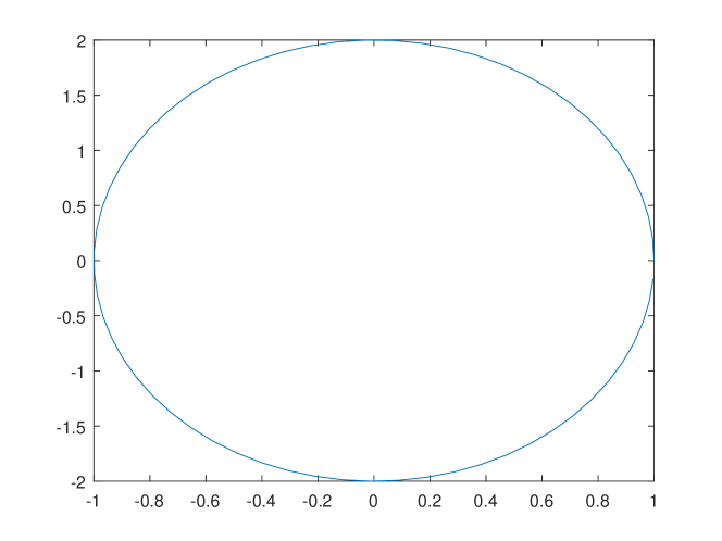
Figure 1: $\Omega$ for Example 5.1

Now

$$k(t,s)=-\frac{1}{2\pi}\ln\frac{(\cos t-\cos s)^{2}+4(\sin t-\sin s)^{2}}{4\sin^{2}(\frac{t-s}{2})},\quad t\neq s,$$

$$k(t,t)=-\frac{1}{2\pi}\ln(\sin^{2}s+4\cos^{2}s),\quad 0\leq t\leq 2\pi,$$

$$2G_{3}(t)=-\frac{1}{|\partial\Omega|}(-\frac{1}{2\pi}\int^{2\pi}_{0}\ln(4\sin^{2}(\frac{t-\sigma}{2}))\sqrt{\sin^{2}\sigma+4\cos^{2}\sigma}d\sigma$$

$$-\frac{1}{2\pi}\int^{2\pi}_{0}\ln\frac{(\cos t-\cos\sigma)^{2}+4(\sin t-\sin\sigma)^{2}}{4\sin^{2}(\frac{t-\sigma}{2})}\sqrt{\sin^{2}\sigma+4\cos^{2}\sigma}d\sigma)$$

$$+\frac{2}{|\partial\Omega|},\quad t\in[0,2\pi].$$

The following experiments are for modified Symm’s integral equation of the first kind: Table 1-6.

	$n$	$2$	$4$	$6$	$8$	10	12
$\delta=0$	$r$	$3.6082$	$0.3327$	$0.0161$	$4.7465e^{-4}$	$2.0573e^{-5}$	$2.0573e^{-5}$
$\delta=0.001$	$r$	$3.6082$	$0.3327$	$0.0161$	$0.0060$	$0.0060$	$0.0060$
$\delta=0.01$	$r$	$3.6082$	$0.3327$	$0.0161$	$0.0601$	$0.0601$	$0.0601$
$\delta=0.1$	$r$	$3.6082$	$0.3327$	$0.0161$	$0.6008$	$0.6008$	$0.6008$

Table 1: Least squares method for Example 5.1

	$n$	$2$	$4$	$6$	$8$	10	12
$\delta=0$	$r$	$3.6082$	$0.3327$	$0.0161$	$4.7465e^{-4}$	$2.0573e^{-5}$	$2.0635e^{-5}$

Table 2: Dual least squares method for Example 5.1.

	$n$	$2$	$4$	$6$	$8$	10	12
$\delta=0$	$r$	$3.6082$	$0.3327$	$0.0161$	$4.7465e^{-4}$	$2.0573e^{-5}$	$2.0573e^{-5}$
$\delta=0.001$	$r$	$3.6082$	$0.3327$	$0.0161$	$0.0060$	$0.0060$	$0.0060$
$\delta=0.01$	$r$	$3.6082$	$0.3327$	$0.0161$	$0.0601$	$0.0601$	$0.0601$
$\delta=0.1$	$r$	$3.6082$	$0.3327$	$0.0161$	$0.6008$	$0.6008$	$0.6008$

Table 3: Bubnov-Galerkin method for Example 5.1.

	$n$	$2$	$4$	$6$	$8$	10	12
$\delta=0$	$r$	$3.7405$	$0.3828$	$0.0197$	$6.0457e^{-4}$	$2.0573e^{-5}$	$2.0573e^{-5}$
$\delta=0.001$	$r$	$3.7405$	$0.3828$	$0.0197$	$0.0060$	$0.0060$	$0.0060$
$\delta=0.01$	$r$	$3.7405$	$0.3834$	$0.0197$	$0.0601$	$0.0601$	$0.0601$
$\delta=0.1$	$r$	$3.7405$	$0.4440$	$0.0197$	$0.6008$	$0.6008$	$0.6008$

Table 4: Galerkin-collocation method for Example 5.1.

			LS	DLS	BG	GC
$\delta=0$	$n=20$	$r$	$2.1222e^{-5}$	$294.4241$	$2.0973e^{-5}$	$2.0573e^{-5}$

Table 5: Additional experiments for PG and GC methods on Example 5.1 with $n=20$

		$n$	$2$	$4$	$6$	$8$	10	12
LS		$t$	17.2271	59.4760	135.8122	237.7139	382.7361	551.4632
DLS		$t$	11.4329	33.0316	72.4827	126.1410	191.6831	323.8654
BG		$t$	12.3776	36.2908	83.5639	139.8100	226.9250	325.4071
GC		$t$	4.4151	6.3802	9.2605	12.5734	14.6543	16.655

Table 6: $t$ denotes the CPU time $(s)$

The following experiments are for corresponding exterior Dirichlet problem of Laplace equation: Table 7, 8.

	$n$	$10^{2}$	$10^{4}$	$10^{6}$	$10^{8}$	$10^{10}$
$d_{1}=(1,0)$	$u_{\infty}$	6.3301	6.3310	6.3312	6.3314	6.3316
	LS: $|u_{\infty}-u^{n}_{\infty}|$	$0.0324e^{-3}$	$0.0680e^{-3}$	$0.1036e^{-3}$	$0.1391e^{-3}$	$0.1747e^{-3}$
	DLS: $|u_{\infty}-u^{n}_{\infty}|$	$0.0324e^{-3}$	$0.0680e^{-3}$	$0.1036e^{-3}$	$0.1391e^{-3}$	$0.1747e^{-3}$
	BG: $|u_{\infty}-u^{n}_{\infty}|$	$0.0324e^{-3}$	$0.0680e^{-3}$	$0.1036e^{-3}$	$0.1391e^{-3}$	$0.1747e^{-3}$
	GC: $|u_{\infty}-u^{n}_{\infty}|$	$0.0324e^{-3}$	$0.0680e^{-3}$	$0.1036e^{-3}$	$0.1391e^{-3}$	$0.1747e^{-3}$

Table 7: $u_{\infty}$ show the behavior of solution to Exterior problem of Laplace equation, the others are the error between solution and approximate solution at infinity.

	$n$	$2$	$4$	$6$	$8$
LS	$Err$	$0.1208$	$0.0064$	$2.2890e^{-5}$	$2.2881e^{-5}$
DLS	$Err$	$0.1203$	$0.0064$	$2.2881e^{-5}$	$2.2881e^{-5}$
BG	$Err$	$0.1203$	$0.0064$	$2.2881e^{-5}$	$2.2881e^{-5}$
GC	$Err$	$0.6812$	$0.0042$	$2.3354e^{-4}$	$2.2881e^{-5}$

Table 8: $Err$ denotes the error between solution and approximate solutions near the boundary $\partial\Omega$

Example 5.2

Let the boundary $\partial\Omega$ of $\Omega$ be parameterized by $\gamma(t)=(e^{-1+\cos t},2e^{-1+\sin t}),\ t\in[0,2\pi]$. We know that $\Omega$ is bounded and simply connected with non-zero tangent vector in every point of $\partial\Omega$. The $\partial\Omega$ is described as

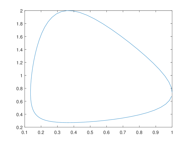
Figure 2: $\Omega$ for Example 5.2

Now

$$k(t,s)=-\frac{1}{2\pi}\ln\frac{(e^{-1+\cos t}-e^{-1+\cos s})^{2}+(2e^{-1+\sin t}-2e^{-1+\sin s})^{2}}{4\sin^{2}(\frac{t-s}{2})},\quad t\neq s,$$

$$k(t,t)=-\frac{1}{2\pi}\ln(e^{-2+2\cos t}\sin^{2}t+4e^{-2+2\sin t}\cos^{2}t),\quad 0\leq t\leq 2\pi,$$

$$2G_{3}(t)=-\frac{1}{|\partial\Omega|}(-\frac{1}{2\pi}\int^{2\pi}_{0}\ln(4\sin^{2}(\frac{t-\sigma}{2}))$$

$$\sqrt{e^{-2+2\cos\sigma}\sin^{2}\sigma+4e^{-2+2\sin\sigma}\cos^{2}\sigma}d\sigma$$

$$-\frac{1}{2\pi}\int^{2\pi}_{0}\ln\frac{(\cos t-\cos\sigma)^{2}+4(\sin t-\sin\sigma)^{2}}{4\sin^{2}(\frac{t-\sigma}{2})}$$

$$\sqrt{e^{-2+2\cos\sigma}\sin^{2}\sigma+4e^{-2+2\sin\sigma}\cos^{2}\sigma}d\sigma)$$

$$+\frac{2}{|\partial\Omega|},\quad t\in[0,2\pi].$$

The following experiments are for modified Symm’s integral equation of the first kind: Table 9-14.

	$n$	$2$	$4$	$6$	$8$	10	12
$\delta=0$	$r$	$0.0588$	$7.1196e^{-4}$	$4.7592e^{-6}$	$2.2762e^{-6}$	$2.2762e^{-6}$	$2.2762e^{-6}$
$\delta=0.001$	$r$	$0.0588$	$7.1143e^{-4}$	$1.9955e^{-4}$	$0.0062$	$0.0062$	$0.0062$
$\delta=0.01$	$r$	$0.0588$	$7.6825e^{-4}$	$0.0020$	$0.00617$	$0.00617$	$0.00617$
$\delta=0.1$	$r$	$0.0589$	$0.0032$	$0.0200$	$0.6171$	$0.6173$	$0.6173$

Table 9: Least squares method for Example 5.2

	$n$	$2$	$4$	$6$	$8$	10	12
$\delta=0$	$r$	$0.0617$	$0.0017$	$1.3082e^{-5}$	$3.0236e^{-6}$	$2.7641e^{-6}$	$1.0268e^{-5}$

Table 10: Dual least squares method for Example 5.2.

	$n$	$2$	$4$	$6$	$8$	10	12
$\delta=0$	$r$	$0.0585$	$7.1098e^{-4}$	$4.7584e^{-6}$	$2.2762e^{-6}$	$2.2762e^{-6}$	$2.2762e^{-5}$
$\delta=0.001$	$r$	$0.0585$	$7.1098e^{-4}$	$4.7584e^{-6}$	$0.0062$	$0.0062$	$0.0062$
$\delta=0.01$	$r$	$0.0585$	$7.1098e^{-4}$	$4.7584e^{-6}$	$0.00617$	$0.00617$	$0.00617$
$\delta=0.1$	$r$	$0.0585$	$7.1098e^{-4}$	$4.7584e^{-6}$	$0.6172$	$0.6173$	$0.6173$

Table 11: Bubnov-Galerkin method for Example 5.2.

	$n$	$2$	$4$	$6$	$8$	10	12
$\delta=0$	$r$	$0.0610$	$8.2528e^{-4}$	$5.5614e^{-6}$	$2.2762e^{-6}$	$2.2762e^{-6}$	$2.2762e^{-5}$
$\delta=0.001$	$r$	$0.0610$	$0.0027$	$5.5614e^{-6}$	$0.0062$	$0.0062$	$0.0062$
$\delta=0.01$	$r$	$0.0610$	$0.0261$	$5.5614e^{-6}$	$0.00617$	$0.00617$	$0.00617$
$\delta=0.1$	$r$	$0.0610$	$0.2611$	$5.5614e^{-6}$	$0.6171$	$0.6173$	$0.6173$

Table 12: Galerkin-Collocation method for Example 5.2.

			LS	DLS	BG	GC
$\delta=0$	$n=20$	$r$	$2.2882e^{-6}$	$51.0699$	$2.2762e^{-6}$	$2.2762e^{-6}$

Table 13: Additional experiments for PG and GC methods on Example 5.2 with $n=20$

		$n$	$2$	$4$	$6$	$8$	10	12
LS		$t$	17.6847	66.6814	133.0920	246.4948	368.4255	519.1206
DLS		$t$	12.8491	36.1843	80.9006	137.3488	209.8712	305.0765
BG		$t$	11.7570	39.6350	87.0154	168.0406	236.5605	387.6846
GC		$t$	4.5987	8.0825	10.8370	12.1855	15.2162	18.5333

Table 14: $t$ denotes the CPU time $(s)$

The following experiments are for corresponding exterior Dirichlet problem of Laplace equation: Table 15,16.

	$n$	$10^{2}$	$10^{4}$	$10^{6}$	$10^{8}$	$10^{10}$
$d_{1}=(1,0)$	$u_{\infty}$	2.7535	2.7544	2.7545	2.7545	2.7545
	LS: $|u_{\infty}-u^{n}_{\infty}|$	$0.1259e^{-4}$	$0.2411e^{-4}$	$0.3561e^{-4}$	$0.4711e^{-4}$	$0.5861e^{-4}$
	DLS: $|u_{\infty}-u^{n}_{\infty}|$	$0.1259e^{-4}$	$0.2411e^{-4}$	$0.3561e^{-4}$	$0.4711e^{-4}$	$0.5861e^{-4}$
	BG: $|u_{\infty}-u^{n}_{\infty}|$	$0.1259e^{-4}$	$0.2411e^{-4}$	$0.3561e^{-4}$	$0.4711e^{-4}$	$0.5861e^{-4}$
	GC: $|u_{\infty}-u^{n}_{\infty}|$	$0.1373e^{-4}$	$0.2525e^{-4}$	$0.3675e^{-4}$	$0.4825e^{-4}$	$0.5975e^{-4}$

Table 15: $u_{\infty}$ show the behavior of solution to Exterior problem of Laplace equation, the others are the error between solution and approximate solution at infinity.

	$n$	$2$	$4$	$6$	$8$
LS	$Err$	$0.0019$	$1.1127e^{-5}$	$9.4236e^{-6}$	$9.4233e^{-6}$
DLS	$Err$	$0.0039$	$3.3159e^{-5}$	$9.4233e^{-6}$	$9.4233e^{-6}$
BG	$Err$	$0.0013$	$1.1366e^{-5}$	$9.4233e^{-6}$	$9.4233e^{-6}$
GC	$Err$	$0.0093$	$1.0659e^{-5}$	$9.4233e^{-6}$	$9.4233e^{-6}$

Table 16: $Err$ denotes the error between solution and approximate solutions near the boundary $\partial\Omega$.

With observations on above numerical results, we see that

• the dual least squares methods is instable and should not be chosen for practical computation, see Table 5, 13.

• the least squares method, Bubnov-Galerkin, Galerkin-Collocation methods perform well with almost the same precision.

• The Galerkin-Collocation methods is much more efficient than PG methods.

• all approximate solutions induced by PG and GC methods to exterior Dirichlet problem satisfy the uniform convergence at infinity.

6 Conclusion

In this paper, on the assumption that the boundary $\partial\Omega$ is analytic, we extend the regular error analysis result from Symm’s integral equation to modified Symm’s integral equation. Besides, inheriting the quadrature technique to handle the singularity in Symm’s integral equation, we establish the numerical procedures of Petrov-Galerkin and Galerkin-Collocation methods with trigonometric interpolation basis on (1.7). We compare the efficiency, precision between above four numerical methods, show the instability of dual least squares method, and examine the precision of single layer approach with different projection methods to exterior Dirichlet problem of Laplace equation and the behavior of solution at infinity.

References

References

- [1] C. Carstensen, E. P. Stephan: Adaptive boundary element methods for some first kind. SIAM J. Numer. Anal. Vol. 33, No. 6, 2166-2183 (1996)
- [2] C. Carstensen, M. Maischak, E. P. Stephan : A posteriori error estimate and h-adaptive algorithm on surfaces for Symm s integral equation. Numer. Math. 90: 197-213 (2001).
- [3] C. Carstensen, D. Praetorius: A posteriori error control in adaptive qualocation boundary element analysis for a logarithmickernel integral equation of the first kind. SIAM J. Sci. Comput. Vol. 25, No. 1, pp. 259-283 (2003).
- [4] C. Carstensen, D. Praetorius: Averaging techniques for the effective numerical solution of Symm’s integral equation of the first kind. SIAM J. Sci. Comput. Vol. 27, No. 4, pp. 1226-1260 (2006).
- [5] G.A. Chandler I, I.H. Sloan: Spline qualocation methods for boundary integral equations, Numer. Math. 58, 537-567 (1990)
- [6] R. Dautray, J. L. Lions: Mathematical Analysis and Numerical Methods for Science and Technology: Volume 1, Physical Origins and Classical Methods. Springer-Verlag Berlin Heidelberg 1990, 2000.
- [7] J. Elschner, I.G. Graham: An optimal order collocation method for first kind boundary integral equations on polygons. Numer. Math. 70: 1-31 (1995)
- [8] J. Elschner, I.G. Graham: Quadrature methods for Symm’s integral equation on polygons. IMA Journal of Numerical Analysis 17, 643-664 (1997).
- [9] M. Faustmann, J. M. Melenk: Local convergence of the boundary element method on polyhedral domains. Numer. Math. 140:593-637 (2018).
- [10] T. Gantumur: Adaptive boundary element methods with convergence rates. Numer. Math. 124:471-516, (2013).
- [11] H. Harbrecht, S. Pereverzev, R. Schneider:Self-regularization by projection for noisy pseudodifferential equations of negative order. Numer. Math. 95: 123-143, (2003).
- [12] S. Joe, Y. Yan:A piecewise constant collocation method using cosine mesh grading for Symm’s equation. Numer. Math. 65, 423-433 (1993).
- [13] A. Kirsch: An Introduction to the Mathematical Theory of Inverse Problems. Springer, New York, 1996.
- [14] R. Kress: Boundary integral equations in time-harmonic acoustic scattering. Math. Comput. Modelling. Vol. 15, No. 3-5, pp. 229-243, 1991.
- [15] R. Kress: Linear integral equations Third edition. Springer-verlag, New York, 2014.
- [16] C. Laurita: A numerical method for the solution of exterior Neumann problems for the Laplace equation in domains with corners Applied Numerical Mathematics 119 (2017) 248-270.
- [17] J. Levesleyf, D. M. Hough:A Chebysbev collocation method for solving Symm’s integral equation for conformal mapping: a partial error analysis. IMA Journal of Numerical Analysis 14, 57-79, (1993).
- [18] W. Mclean, I. H. Sloan:A fully discrete and symmetric boundary element method. IMA Journal of Numerical Analysis 14, 311-345, (1994).
- [19] G. Monegato, L. Scuderi:Global polynomial approximation for Symm s equation on polygons. Numer. Math. 86: 655-683, (2000).
- [20] J. Saranen:The convergence of even degree spline collocation solution for potential problems in smooth domains of the plane. Numer. Math. 53, 499-512, (1988).
- [21] Olha Ivanyshyn Yaman, Gazi Ozdemir: Boundary integral equations for the exterior Robin problem in two dimensions Applied Mathematics and Computation Volume 337, 15 November 2018, Pages 25-33
- [22] Y. Yan, I. H. Sloan:On integral equations of the first kind with logarithmic kernels. Journal Of Integral Equations And Applications Volume 1, Number 4, 549-579, (1988).