Generation of quantum entangled states of multiple groups of qubits distributed in multiple cavities

Abstract

Provided that cavities are initially in a Greenberger-Horne-Zeilinger (GHZ) entangled state, we show that GHZ states of $N$-group qubits distributed in $N$ cavities can be created via a 3-step operation. The GHZ states of the $N$-group qubits are generated by using $N$-group qutrits placed in the $N$ cavities. Here, “qutrit” refers to a three-level quantum system with the two lowest levels representing a qubit while the third level acting as an intermediate state necessary for the GHZ state creation. This proposal does not depend on the architecture of the cavity-based quantum network and the way for coupling the cavities. The operation time is independent of the number of qubits. The GHZ states are prepared deterministically because no measurement on the states of qutrits or cavities is needed. In addition, the third energy level of the qutrits during the entire operation is virtually excited and thus decoherence from higher energy levels is greatly suppressed. This proposal is quite general and can in principle be applied to create GHZ states of many qubits using different types of physical qutrits (e.g., atoms, quantum dots, NV centers, various superconducting qutrits, etc.) distributed in multiple cavities. As a specific example, we further discuss the experimental feasibility of preparing a GHZ state of four-group transmon qubits (each group consisting of three qubits) distributed in four one-dimensional transmission line resonators arranged in an array.

I. INTRODUCTION AND MOTIVATION

Large-scale quantum information processing (QIP) has drawn much attention [1-3]. Usually, a large number of qubits may be involved in large-scale QIP. The size of QIP with qubits in multiple cavities can be larger when compared to QIP with qubits in a single cavity. For instance, given the number of qubits in each cavity is $m$, the number of qubits placed in $n$ cavities is $n\times m$, which is $n$ times the number $m$ of qubits placed in a single cavity. Therefore, large-scale QIP based on cavity or circuit QED may require distributing qubits in different cavities. In such an architecture, quantum state engineering and manipulation may involve not only qubits in the same cavity but also qubits distributed in different cavities [4,5]. The ability to prepare quantum entangled states of qubits located in different cavities and to perform nonlocal quantum operations on qubits in different cavities is a prerequisite to realize large-scale QIP based on cavity or circuit QED [6,7].

Greenberger-Horne-Zeilinger (GHZ) entangled states play a key role in quantum communication and QIP. To give just a few examples, QIP [8], quantum communication [9-11], error-correction protocols [12,13], quantum metrology [14], and high-precision spectroscopy [15,16] require entangling quantum systems in a GHZ state. New systems and methods for preparing and measuring GHZ states have therefore been sought intensively for a long time, and remains a very active field of research. To date, GHZ states of 10 or more qubits have been experimentally demonstrated in various systems. For examples, experiments have reported the generation of GHZ states with 14 ionic qubits [17], 20 atomic qubits [18], 12 photonic qubits via a linear optical setup [19], 18 qubits with six photons’ three degrees of freedom [20], and 10 superconducting (SC) qubits coupled to a single microwave resonator [21]. Moreover, GHZ states of 18 SC qubits coupled to a single cavity or resonator has recently been produced in experiments [22] (hereafter, the terms cavity and resonator are used interchangeably). Theoretically, based on cavity or circuit QED, a large number of theoretical methods have been presented for creating multi-qubit GHZ states with various quantum systems (e.g., atoms, quantum dots, SC qutrits, NV centers, etc.), which are placed in a single cavity or coupled to a single resonator [23-31]. Moreover, proposals have been presented to entangle qubits distributed in different cavities [32-42]. Note that the previous methods presented for entangling qubits in a single cavity or resonator may not be applied to entangle qubits that are distributed in different cavities, and the previous proposals for entangling qubits in different cavities are not universal, which depend on the specific cavity-system architecture and the way in which the cavities are connected.

Motivated by the above, we present an efficient method to prepare GHZ states of $N$-group qubits distributed in a $N$-cavity system. The multi-qubit GHZ states are generated by using qutrits (three-level quantum systems) placed in cavities or embedded in resonators. Here, the two logic states of a qubit are represented by the two lowest levels of a qutrit placed in a cavity, while the third higher energy level of each qutrit is utilized to facilitate the coherent manipulation. By using this proposal, we show that given the initial GHZ state of the cavities is prepared, the $N$-group qubits can be deterministically prepared in a GHZ state with a 3-step operation only. The procedure for creating the GHZ state of qubits works for a 1D (one-dimensional), 2D, or 3D cavity-based quantum network (Fig. 1). Moreover, it does not depend on in which way the cavities are connected (e.g., via optical fibers or other auxiliary systems). This proposal is quite general and can be used to create GHZ states of multiple groups of qubits, by using natural atoms or artificial atoms (e.g., quantum dots, NV centers, various SC qutrits, etc.) distributed in different cavities.

Other advantages of this proposal are: (i) The GHZ state is prepared in a deterministic way because neither measurement on the state of qutrits nor measurement on the state of the cavities is needed; (ii) The GHZ-state preparation time is independent of the number of qubits and thus does not increase with the number of qubits; and (iii) The third level $\left|f\right\rangle$ of the qutrits is not occupied during the entire operation, thus decoherence from the higher energy levels of the qutrits is greatly suppressed.

As an example, we further discuss the experimental feasibility of the proposal, based on circuit QED. Our numerical simulations show that within current circuit QED technology, it is feasible to produce GHZ states of four groups of SC transmon qubits, each group containing three transmon qubits and the four groups distributed in four one-dimensional transmission line resonators (TLRs) arranged in an array. By increasing the number of resonators, GHZ states of more groups of SC qubits can be created experimentally.

This paper is organized as follows. Sec. II introduces basic theory. Sec. III shows how to generate GHZ states of $N$-group qubits distributed in $N$cavities. Sec. IV investigates the experimental feasibility of preparing GHZ states of four-group SC transmon qubits distributed in four TLRs arranged in an array. A concluding summary is given in Sec. V.

II. BASIC THEORY

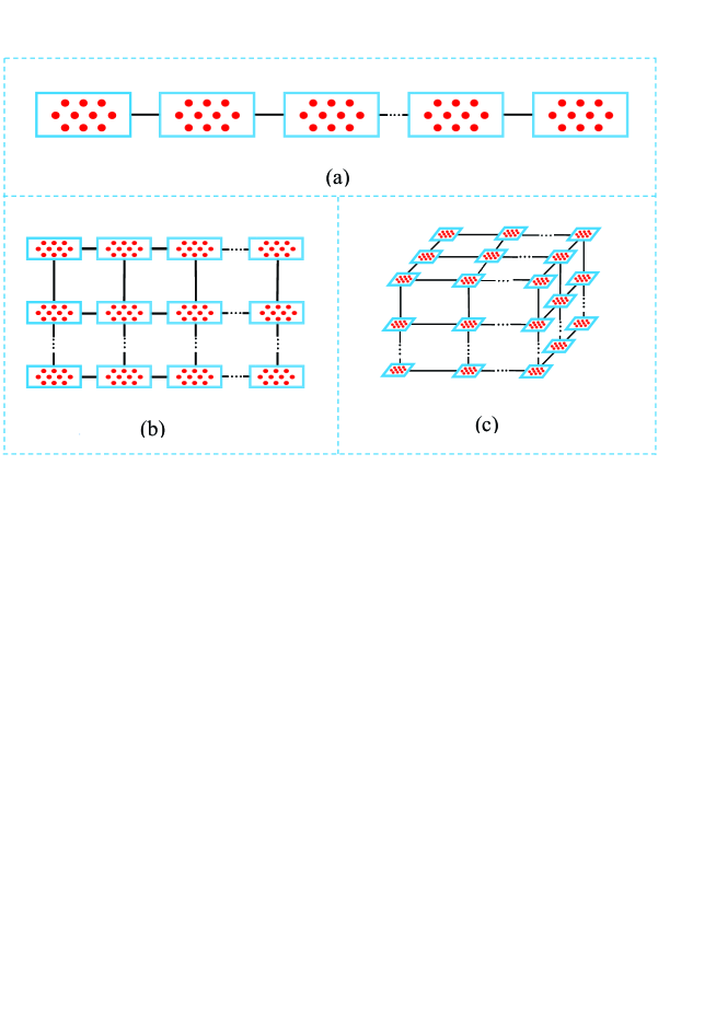
Figure 1: (color online) (a) 1D cavity-based quantum network. (b) 2D cavity-based quantum network. (c) 3D cavity-based quantum network. In (a,b,c), each short line represents an optical fiber or other auxiliary system, which is used to couple two adjacent cavities. In addition, each cavity is a 1D or 3D cavity, hosting one group of qutrits (red dots).

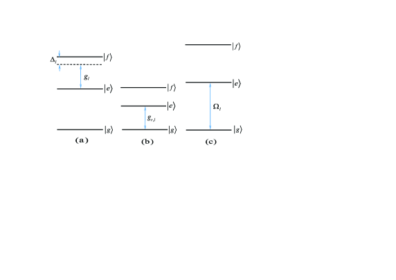
Figure 2: (color online) (a) Illustration of the dispersive interaction between cavity $l$ and the $\left|e\right\rangle$ $\leftrightarrow$ $\left|f\right\rangle$ transition of qutrits $\left\{1_{l},2_{l},...,\left(m-1\right)_{l}\right\}$, with coupling constant $g_{l}$ and detuning $\Delta_{l}=\omega_{fe}-\omega_{c_{l}}>0$. Here, $\omega_{fe}$ is the $\left|e\right\rangle$ $\leftrightarrow$ $\left|f\right\rangle$ transition frequency of the qutrits and $\omega_{c_{l}}$ is the frequency of cavity $l$. (b) Illustration of the resonant interaction between cavity $l$ and the $\left|g\right\rangle$ $\leftrightarrow$ $\left|e\right\rangle$ transition of qutrit $m_{l}$ with coupling constant $g_{r,l}$. (c) Illustration of the resonant interaction between a classical pulse and the $\left|g\right\rangle$ $\leftrightarrow$ $\left|e\right\rangle$ transition of qutrits $\left\{1_{l},2_{l},...,\left(m-1\right)_{l}\right\}$ in cavity $l$. Note that the level structures in (a), (b), and (c) are different. The level spacings of qutrits in (a) are adjusted such that $\left|e\right\rangle\leftrightarrow\left|f\right\rangle$ transition is dispersively coupled to cavity $l$. The level spacings in (b) are adjusted such that the $\left|g\right\rangle\leftrightarrow\left|e\right\rangle$ transition is resonant with cavity $l$. The level spacings in (c) are adjusted such that qutrits are decoupled from cavity $l$ during the pulse. A blue double-arrow vertical line in (a) and (b) represents the frequency of cavity $l$, while a blue double-arrow vertical line in (c) represents the pulse frequency.

Consider $N$ cavities ($1,2,...,N$) each hosting a group of qutrits (Fig. 1). For simplicity, assume that each group contains $m$ qutrits. The $m$ qutrits hosted in cavity $l$ ($l=1,2,...,N$) are labelled as $1_{l},$ $2_{l},...,$ and $m_{l}$. The three levels of each qutrit are denoted as $\left|g\right\rangle,$ $\left|e\right\rangle$ and $\left|f\right\rangle$ (Fig. 2). As shown in the next section, the GHZ state preparation requires: (i) Cavity $l$ dispersively interacting with the $\left|e\right\rangle\leftrightarrow$ $\left|f\right\rangle$ transition of each of qutrits $\left\{1_{l},2_{l},...,\left(m-1\right)_{l}\right\}$ in cavity $l,$ (ii) Cavity $l$ resonantly interacting with the $\left|g\right\rangle\leftrightarrow$ $\left|e\right\rangle$ transition of qutrit $m_{l}$ in cavity $l$, and (iii) A classical pulse resonantly interacting with the $\left|g\right\rangle\leftrightarrow$ $\left|e\right\rangle$ transition of each of qutrits $\left\{1_{l},2_{l},...,\left(m-1\right)_{l}\right\}$ in cavity $l$ ($l=1,2,...,N$). In the following, we will give a brief introduction to the state evolution under these types of interaction.

A. Qutrit-cavity dispersive interaction

Suppose that cavity $l$ is dispersively coupled to the $\left|e\right\rangle$ $\leftrightarrow$ $\left|f\right\rangle$ transition of each of qutrits $\left\{1_{l},2_{l},...,\left(m-1\right)_{l}\right\}$ with coupling strength $g_{l}$ and detuning $\Delta_{l}=\omega_{fe}-\omega_{c_{l}}>0$, while highly detuned (decoupled) from other energy level transitions [Fig. 2(a)]. Here, $\omega_{fe}$ and $\omega_{c_{l}}$ are the $\left|e\right\rangle$ $\leftrightarrow$ $\left|f\right\rangle$ transition frequency of each qutrit and the frequency of cavity $l,$ respectively. This condition can be met by prior adjustment of the qutrit’s level spacings or the frequency of cavity $l$. For instance, the level spacings of superconducting qutrits can be rapidly (within $1\sim 3$ ns) tuned [43,44]; the level spacings of NV centers can be readily adjusted by changing the external magnetic field applied along the crystalline axis of each NV center [45,46]; and the level spacings of atoms/quantum dots can be adjusted by changing the voltage on the electrodes around each atom/quantum dot [47]. In addition, the frequency for an optical cavity can be changed in experiments [48], and the frequency of a microwave cavity can be rapidly adjusted with a few nanoseconds [49,50].

Under the above assumptions, the Hamiltonian of the whole system in the interaction picture and after the rotating wave approximation (RWA) is given by (assuming $\hbar=1$)

$$H_{1}=\sum\limits_{l=1}^{N}g_{l}e^{i\Delta_{l}t}\hat{a}_{l}S_{fe,l}^{+}+\text{H.c.,}$$ (1)

where $S_{fe,l}^{+}=\sum\limits_{j=1}^{m-1}\left|f\right\rangle_{j_{l}}\left\langle e\right|$, and $\hat{a}_{l}$ is the photon annihilation operator of the cavity $l$ ($l=1,2,...,N$). In Eq. (1), we assume that the coupling strength $g_{l}$ between cavity $l$ and the $\left|e\right\rangle$ $\leftrightarrow$ $\left|f\right\rangle$ transition is the same for all of qutrits $\left\{1_{l},2_{l},...,\left(m-1\right)_{l}\right\}.$

Under the large detuning condition $\Delta_{l}\gg g_{l}\ (l=1,2,...,N),$ we can obtain the following effective Hamiltonian [51–53]

$$H_{\mathrm{eff}}=\sum\limits_{l=1}^{N}\lambda_{l}\left(S_{f,l}\hat{a}_{l}\hat{a}_{l}^{+}-S_{e,l}\hat{a}_{l}^{+}\hat{a}_{l}+\sum_{j,k=1;j\neq k}^{m-1}\left|f\right\rangle_{j_{l}}\left\langle e\right|\otimes\left|e\right\rangle_{k_{l}}\left\langle f\right|\right)$$ (2)

where $S_{f,l}=\sum\limits_{j=1}^{m-1}\left|f\right\rangle_{j_{l}}\left\langle f\right|,$ $S_{e,l}=\sum\limits_{j=1}^{m-1}\left|e\right\rangle_{j_{l}}\left\langle e\right|,$ and $\lambda_{l}=g_{l}^{2}/\Delta_{l}.$ Here, the first (second) term is an ac-Stark shift of the level $\left|f\right\rangle$ ($\left|e\right\rangle$) induced by cavity $l$. The last term represents the “dipole” coupling between the $j$th and the $k$th qutrits in cavity $l$, mediated by cavity $l$. When the level $\left|f\right\rangle$ of each qutrit is not occupied, the Hamiltonian (2) reduces to

$$H_{\mathrm{eff}}=-\sum\limits_{l=1}^{N}\lambda_{l}S_{e,l}\hat{a}_{l}^{+}\hat{a}_{l}.$$ (3)

Under this Hamiltonian, one can easily find that the following state evolution

$$\begin{array}[]{c}\left|g\right\rangle_{j_{l}}\left|0\right\rangle_{c_{l}}\\ \left|e\right\rangle_{j_{l}}\left|0\right\rangle_{c_{l}}\\ \left|g\right\rangle_{j_{l}}\left|1\right\rangle_{c_{l}}\\ \left|e\right\rangle_{j_{l}}\left|1\right\rangle_{c_{l}}\end{array}\rightarrow\begin{array}[]{c}\left|g\right\rangle_{j_{l}}\left|0\right\rangle_{c_{l}}\\ \left|e\right\rangle_{j_{l}}\left|0\right\rangle_{c_{l}}\\ \left|g\right\rangle_{j_{l}}\left|1\right\rangle_{c_{l}}\\ e^{i\lambda_{l}t}\left|e\right\rangle_{j_{l}}\left|1\right\rangle_{c_{l}}\end{array}.$$ (4)

applies to each of qutrits $\left\{1_{l},2_{l},...,\left(m-1\right)_{l}\right\}$ in cavity $l$ simultaneously ($l=1,2,...,N$). Note that the subscript $j_{l}$ involved in Eq. (4) is $1_{l},2_{l},...,$or $(m-1)_{l}$ $(l=1,2,...,N)$.

Consider that cavity $l$ is resonant with the $\left|g\right\rangle$ $\leftrightarrow$ $\left|e\right\rangle$ transition of qutrit $m_{l}$ $(l=1,2,...,N)$ [Fig. 2(b)]. The Hamiltonian in the interaction picture and after the RWA is given by

$$H_{2}=g_{r,l}\hat{a}_{l}\left|e\right\rangle_{m_{l}}\left\langle g\right|+\text{H.c.},$$ (5)

where $g_{r,l}$ is the resonant coupling constant of cavity $l$ with the $\left|g\right\rangle$ $\leftrightarrow$ $\left|e\right\rangle$ transition of qutrit $m_{l}.$ Under this Hamiltonian, we can obtain the state evolution

$$\left|g\right\rangle_{m_{l}}\left|1\right\rangle_{c_{l}}\rightarrow\cos g_{r,l}t\left|g\right\rangle_{m_{l}}\left|1\right\rangle_{c_{l}}-i\sin g_{r,l}t\left|e\right\rangle_{m_{l}}\left|0\right\rangle_{c_{l}},$$ (6)

while the state $\left|g\right\rangle_{m_{l}}\left|0\right\rangle_{c_{l}}$ remains unchanged.

Assume that a classical pulse is resonant with the $\left|g\right\rangle$ $\leftrightarrow$ $\left|e\right\rangle$ transition of each of qutrits $\left\{1_{l},2_{l},...,\left(m-1\right)_{l}\right\}$ in cavity $l$ [Fig. 2(c)]. The Hamiltonian in the interaction picture and after making the RWA is given by

$$H_{3}=\Omega_{l}e^{-i\phi}S_{eg,l}^{+}+\text{H.c.},$$ (7)

where $S_{eg,l}^{+}=\sum\limits_{j=1}^{m-1}\left|e\right\rangle_{j_{l}}\left\langle g\right|,$ $\phi$ is the pulse initial phase and $\Omega_{l}$ is the pulse Rabi frequency. Under this Hamiltonian, we can easily obtain the following state rotation

$$\left|g\right\rangle_{j_{l}} \rightarrow \cos\Omega_{l}t\left|0\right\rangle-ie^{-i\phi}\sin\Omega_{l}t\left|1\right\rangle,$$

$$\left|e\right\rangle_{j_{l}} \rightarrow -ie^{i\phi}\sin\Omega_{l}t\left|0\right\rangle+\cos\Omega_{l}t\left|1\right\rangle,$$ (8)

for qutrit $j_{l}$ ($j=1,2,...,m-1$).

The results (4), (6) and (8) will be applied for the GHZ state preparation, as shown in the next section.

III. PREPARATION OF GHZ STATES OF $\mathbf{N}$-GROUP QUBITS IN $\mathbf{N}$ CAVITIES

Assume that the $N$ cavities are initially prepared in a GHZ state $\alpha\left|0\right\rangle_{c_{1}}\left|0\right\rangle_{c_{2}}...\left|0\right\rangle_{c_{N}}+\beta\left|1\right\rangle_{c_{1}}\left|1\right\rangle_{c_{2}}...\left|1\right\rangle_{c_{N}}$ ($\left|\alpha\right|^{2}+\left|\beta\right|^{2}=1,\alpha\neq 0,$ $\beta\neq 0$). In addition, assume that qutrit $m_{l}$ in cavity $l$ is in the state $\left|g\right\rangle$ while each of the remaining qutrits $\left\{1_{l},2_{l},...,\left(m-1\right)_{l}\right\}$ in cavity $l$ is in the state $\frac{1}{\sqrt{2}}$ $\left(\left|g\right\rangle+\left|e\right\rangle\right)$, which can be prepared by applying a classical $\pi$ pulse resonant with the $\left|g\right\rangle$ $\leftrightarrow$ $\left|e\right\rangle$ transition of the qutrits each initially in the state $\left|g\right\rangle.$ Hereafter, define $\left|\pm\right\rangle=\frac{1}{\sqrt{2}}$ $\left(\left|g\right\rangle\pm\left|e\right\rangle\right).$ The initial state of the whole system is thus given by

$$\left(\alpha\left|0\right\rangle_{c_{1}}\left|0\right\rangle_{c_{2}}...\left|0\right\rangle_{c_{N}}+\beta\left|1\right\rangle_{c_{1}}\left|1\right\rangle_{c_{2}}...\left|1\right\rangle_{c_{N}}\right)$$

$$\otimes\prod\limits_{j=1}^{m-1}\left|+\right\rangle_{j_{1}}\prod\limits_{j=1}^{m-1}\left|+\right\rangle_{j_{2}}...\prod\limits_{j=1}^{m-1}\left|+\right\rangle_{j_{N}}\otimes\left|g\right\rangle_{m_{1}}\left|g\right\rangle_{m_{2}}...\left|g\right\rangle_{m_{N}},$$ (9)

where the subscripts $j_{1},j_{2},...,j_{N}$ represent the $j$th qutrit in cavity $1$, cavity $2$, …, cavity $N$ respectively; and $m_{1},m_{2},...m_{N}$ represent the $m$-th qutrit (i.e., qutrit $m$) in cavity $1$, cavity $2$, …, cavity $N$ respectively.

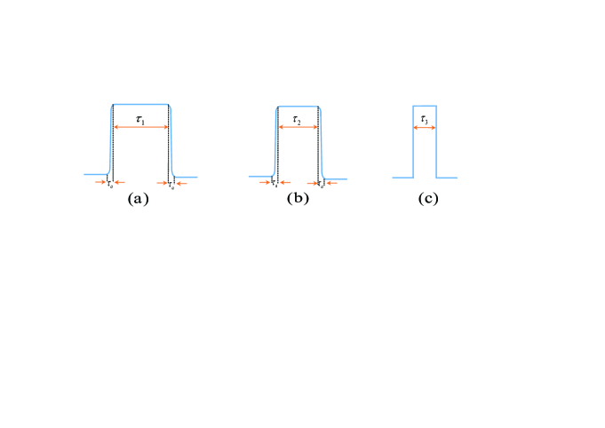
Figure 3: (color online) (a) Sequence of operations for step 1. (b) Sequence of operations for step 2. (c) Sequence of operations for step 3. Here, $\tau_{1}$ and $\tau_{2}$ are the qutrit-cavity interaction times, while $\tau_{3}$ is the qutrit-pulse interaction time, as described in the text. In addition, $\tau_{a}$ is the typical time required to adjust the qutrit level spacings. Note that the operation sequence in (a)-(c) follows from left to right.

All qutrits are initially decoupled from their respective cavities. The procedure for preparing the $N$-group qubits in a GHZ state is listed below:

Step 1. Keep qutrit $m_{l}$ decoupled from cavity $l$ but adjust the level spacing of qutrits $\left\{1_{l},2_{l},...,\left(m-1\right)_{l}\right\}$ in cavity $l$ to obtain an effective Hamiltonian described by Eq. (3). According to Eq. (4), the state (9) evolves as follows

$$\left[\alpha\left|0\right\rangle_{c_{1}}\left|0\right\rangle_{c_{2}}...\left|0\right\rangle_{c_{N}}\otimes\prod\limits_{j=1}^{m-1}\left|+\right\rangle_{j_{1}}\prod\limits_{j=1}^{m-1}\left|+\right\rangle_{j_{2}}...\prod\limits_{j=1}^{m-1}\left|+\right\rangle_{j_{N}}\right.$$

$$\left.+\beta\left|1\right\rangle_{c_{1}}\left|1\right\rangle_{c_{2}}...\left|1\right\rangle_{c_{N}}\prod\limits_{j=1}^{m-1}\frac{\left(\left|g\right\rangle_{j_{1}}+e^{i\lambda_{1}t}\left|e\right\rangle_{j_{1}}\right)}{\sqrt{2}}\prod\limits_{j=1}^{m-1}\frac{\left(\left|g\right\rangle_{j_{2}}+e^{i\lambda_{2}t}\left|e\right\rangle_{j_{2}}\right)}{\sqrt{2}}...\prod\limits_{j=1}^{m-1}\frac{\left(\left|g\right\rangle_{j_{N}}+e^{i\lambda_{N}t}\left|e\right\rangle_{j_{N}}\right)}{\sqrt{2}}\right]$$

$$\otimes\left|g\right\rangle_{m_{1}}\left|g\right\rangle_{m_{2}}...\left|g\right\rangle_{m_{N}}.$$ (10)

By setting $\lambda_{1}=\lambda_{2}=...=\lambda_{N}=\lambda$ and for $t=\tau_{1}=\pi/\lambda,$ the state (10) becomes

$$\left(\alpha\left|0\right\rangle_{c_{1}}\left|0\right\rangle_{c_{2}}...\left|0\right\rangle_{c_{N}}\otimes\prod\limits_{j=1}^{m-1}\left|+\right\rangle_{j_{1}}\prod\limits_{j=1}^{m-1}\left|+\right\rangle_{j_{2}}...\prod\limits_{j=1}^{m-1}\left|+\right\rangle_{j_{N}}\right.$$

$$\left.+\beta\left|1\right\rangle_{c_{1}}\left|1\right\rangle_{c_{2}}...\left|1\right\rangle_{c_{N}}\prod\limits_{j=1}^{m-1}\left|-\right\rangle_{j_{1}}\prod\limits_{j=1}^{m-1}\left|-\right\rangle_{j_{2}}...\prod\limits_{j=1}^{m-1}\left|-\right\rangle_{j_{N}}\right)$$

$$\otimes\left|g\right\rangle_{m_{1}}\left|g\right\rangle_{m_{2}}...\left|g\right\rangle_{m_{N}}.$$ (11)

Then, adjust the level spacings of qutrits $\left\{1_{l},2_{l},...,\left(m-1\right)_{l}\right\}$ such that they are decoupled from cavity $l$. The operation sequence for this step of operation is illustrated in Fig. 3(a).

Step 2. Adjust the level spacing of qutrit $m_{l}$ in cavity $l$ such that the $\left|g\right\rangle$ $\leftrightarrow$ $\left|e\right\rangle$ transition of qutrit $m_{l}$ is resonant with cavity $l$ (with a resonant coupling constant $g_{r,l}$). After an interaction time $\tau_{2}=\pi/\left(2g_{r,l}\right)$, we have $\left|1\right\rangle_{c_{l}}\left|g\right\rangle_{m_{l}}\rightarrow-i\left|0\right\rangle_{c_{l}}\left|e\right\rangle_{m_{l}}$ according to Eq. (6). Thus, the state (11) becomes

$$\left(\alpha\prod\limits_{j=1}^{m-1}\left|+\right\rangle_{j_{1}}\prod\limits_{j=1}^{m-1}\left|+\right\rangle_{j_{2}}...\prod\limits_{j=1}^{m-1}\left|+\right\rangle_{j_{N}}\otimes\left|g\right\rangle_{m_{1}}\left|g\right\rangle_{m_{2}}...\left|g\right\rangle_{m_{N}}\right.$$

$$\left.+\left(-i\right)^{N}\beta\prod\limits_{j=1}^{m-1}\left|-\right\rangle_{j_{1}}\prod\limits_{j=1}^{m-1}\left|-\right\rangle_{j_{2}}...\prod\limits_{j=1}^{m-1}\left|-\right\rangle_{j_{N}}\otimes\left|e\right\rangle_{m_{1}}\left|e\right\rangle_{m_{2}}...\left|e\right\rangle_{m_{N}}\right)$$

$$\otimes\left|0\right\rangle_{c_{1}}\left|0\right\rangle_{c_{2}}...\left|0\right\rangle_{c_{N}}.$$ (12)

To maintain the state (12), one should adjust the level spacing of qutrit $m_{l}$ such that it is decoupled from cavity $l.$ The operation sequence for this step of operation is illustrated in Fig. 3(b).

Step 3. Apply a classical $\pi$ pulse (with an initial phase $\pi/2$) to qutrit $j_{l}$ ($j=1,2,...,m-1$). The pulse is resonant with the $\left|g\right\rangle$ $\leftrightarrow$ $\left|e\right\rangle$ transition of qutrit $j_{l}$ for a duration time $\tau_{3}=\pi/\left(2\Omega_{l}\right),$ resulting in $\left|+\right\rangle_{j_{l}}\rightarrow\left|g\right\rangle_{j_{l}}$ and $\left|-\right\rangle_{j_{l}}\rightarrow-\left|e\right\rangle_{j_{l}}$ according to Eq. (8). The state (12) thus becomes

$$\alpha\prod\limits_{j=1}^{m}\left|g\right\rangle_{j_{1}}\prod\limits_{j=1}^{m}\left|g\right\rangle_{j_{2}}...\prod\limits_{j=1}^{m}\left|g\right\rangle_{j_{N}}+e^{i\phi}\beta\prod\limits_{j=1}^{m}\left|e\right\rangle_{j_{1}}\prod\limits_{j=1}^{m}\left|e\right\rangle_{j_{2}}...\prod\limits_{j=1}^{m}\left|e\right\rangle_{j_{N}},$$ (13)

where $\phi=\left(m-3/2\right)N\pi.$ This state is a GHZ entangled state for the $N$-group qubits in the $N$ cavities, with the two logic states of a qubit being represented by the two lowest levels $\left|g\right\rangle$ and $\left|e\right\rangle$ of a qutrit. For $\left|\alpha\right|=\left|\beta\right|=1/\sqrt{2},$ the state (13) is a standard GHZ state with maximal entanglement. The operation sequence for this step of operation is illustrated in Fig. 3(c).

In above, we have set $\lambda_{1}=\lambda_{2}=...=\lambda_{N}$, which turns out into

$$\frac{g_{1}^{2}}{\Delta_{1}}=\frac{g_{2}^{2}}{\Delta_{2}}=...=\frac{g_{N}^{2}}{\Delta_{N}}.$$ (14)

This condition (14) can be readily met by adjusting the qutrits’ positions in the cavities, the qutrits’ level spacings [43-47] or the cavity frequencies [48-50].

From the above description, one can see:

(i) Because the same detuning $\Delta_{l}$ is set for each of qutrits $1_{l},2_{l},...,\left(m-1\right)_{l}$ in cavity $l$ ($l=1,2,...,N$), the level spacings for qutrits $1_{l},2_{l},...,\left(m-1\right)_{l}$ can be synchronously adjusted, e.g., via changing the common external parameters.

(ii) During the entire operation, the level $\left|f\right\rangle$ for all qutrits in each cavity is not occupied. Thus, decoherence due to energy relaxation and dephasing of this higher energy level is greatly suppressed.

(iii) Assume that both $g_{r,1},g_{r,2},...,g_{r,N}$ and $\Omega_{1},\Omega_{2},...,\Omega_{N}$ are non-identical for different cavities. Thus, the total operation time is

$$t_{op}=\pi/\lambda+\max\{\frac{\pi}{2g_{r,1}},\frac{\pi}{2g_{r,2}},...,\frac{\pi}{2g_{r,N}}\}+\max\{\frac{\pi}{2\Omega_{1}},\frac{\pi}{2\Omega_{2}},...,\frac{\pi}{2\Omega_{N}}\}+4\tau_{d},$$ (15)

which is independent of the number of qubits and thus does not increase with the number of qubits. Note that $\tau_{d}$ is the typical time required for adjusting the level spacings of qutrits.

(iv) This proposal does not require measurement on the state of the qutrits or the cavities. Thus, the GHZ state is created deterministically.

(v) The above operations have nothing to do with the manner in which the cavities are connected. In this sense, the method presented here can be applied to create GHZ states of the qubits distributed in a 1D, 2D, or 3D cavity-based quantum network (Fig. 1), where the cavities can be connected with optical fibers or other auxiliary systems.

(vi) When the $N$ cavities are initially prepared in another type of symmetrical GHZ state $\alpha\left|0\right\rangle_{c_{1}}\left|0\right\rangle_{c_{2}}...\left|0\right\rangle_{c_{s}}\left|1\right\rangle_{c_{s+1}}\left|1\right\rangle_{c_{s+2}}...\left|1\right\rangle_{c_{N}}+\beta\left|1\right\rangle_{c_{1}}\left|1\right\rangle_{c_{2}}...\left|1\right\rangle_{c_{s}}\left|0\right\rangle_{c_{s+1}}\left|0\right\rangle_{c_{s+2}}...\left|0\right\rangle_{c_{N}},$ it is straightforward to show that by following the procedure described above, the $N$-group qubits distributed in $N$ cavities will be prepared in the following GHZ state

$$\alpha\prod\limits_{j=1}^{m}\left|g\right\rangle_{j_{1}}\prod\limits_{j=1}^{m}\left|g\right\rangle_{j_{2}}...\prod\limits_{j=1}^{m}\left|g\right\rangle_{j_{s}}\prod\limits_{j=1}^{m}\left|e\right\rangle_{j_{s+1}}\prod\limits_{j=1}^{m}\left|e\right\rangle_{j_{s+2}}...\prod\limits_{j=1}^{m}\left|e\right\rangle_{j_{N}}$$

$$+\beta\prod\limits_{j=1}^{m}\left|e\right\rangle_{j_{1}}\prod\limits_{j=1}^{m}\left|e\right\rangle_{j_{2}}...\prod\limits_{j=1}^{m}\left|e\right\rangle_{j_{s}}\prod\limits_{j=1}^{m}\left|g\right\rangle_{j_{s+1}}\prod\limits_{j=1}^{m}\left|g\right\rangle_{j_{s+2}}...\prod\limits_{j=1}^{m}\left|g\right\rangle_{j_{N}}.$$ (16)

(vii) The procedure described above can also be applied to create GHZ state of $N-$ group qubits distributed in $N$ cavities in the case when the number of qutrits in each group is different.

As a matter of fact, the condition (14) is unnecessary. For the case of $\lambda_{1}\neq\lambda_{2}\neq...\neq\lambda_{N}$, the state (11) resulting from the operation of step 1 described above cannot be achieved by turning on/off the effective couplings of the qutrits with the $N$ cavities simultaneously. However, this state (11) can be obtained by modifying the operation of step 1 as follows. First, switch on the effective dispersive interaction of the qutrits $\{1_{l},2_{l},...,\left(m-1\right)_{l}\}$ with cavity $l$ at a proper time $\tau_{l}$ = $t_{\max}-t_{l},$ by tuning the frequency of the qutrits $\{1_{l},2_{l},...,\left(m-1\right)_{l}\}$ or the frequency of cavity $l$ to have the proper $\Delta_{l},$ where $t_{\max}$ $=\max\{\pi/\left(2\lambda_{1}\right),\pi/\left(2\lambda_{2}\right),...,\pi/\left(2\lambda_{N}\right)\}$ and $t_{l}=$ $\pi/\left(2\lambda_{l}\right)$. Then, switch off all the effective interactions of the qutrits with the $N$ cavities at the time $t_{\max},$ by tuning the frequency of the qutrits or the frequency of the $N$ cavities such that the qutrits are decoupled from the $N$ cavities.

In the above discussion, we have assumed that the coupling strength $g_{l}$ is identical for all of qutrits $\{1_{l},2_{l},...,\left(m-1\right)_{l}\}$ in cavity $l$ ($l=1,2,...,N)$. For the case of $g_{l}$ varying with different qutrits in cavity $l,$ this proposal is still valid as long as the large detuning condition holds for individual qutrits, but the procedure may become more complex because one will need to adjust the frequencies of individual qutrits separately. Therefore, to simplify the experiments, it is strongly suggested to design the sample with identical qutrit-cavity coupling strength for qutrits in the same cavity.

To prepare the cavities in the GHZ state, two key ingredients are required. One is the coupling between neighbor cavities. For optical cavities, this can be obtained by using optical fibers to connect the neighbor cavities. In addition, for microwave cavities or resonators, this can be achieved by using solid-state auxiliary systems (e.g., superconducting qubits/qutrits, quantum dots, or NV centers) to connect the neighbor cavities. The other is decoupling of the intra-cavity atoms with the cavities. This can be realized by adjusting the level spacings of the atoms or the frequencies of the cavities such that the cavities are highly detuned (decoupled) from the transitions between any two levels of the atoms. As discussed previously, both level spacings of natural or artificial atoms and cavity frequencies can be adjusted in experiments [43-50].

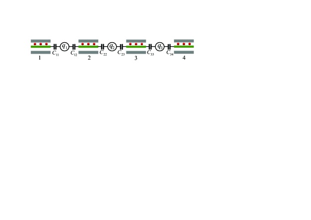
Figure 4: (color online) 1D quantum network consisting of four one-dimensional transmission line resonators (TLRs) arranged in an array. Each TLR hosts three SC transmon qutrits (red dots), and adjacent TLRs are coupled through SC transmon qutrits ($q_{1},q_{2},q_{3}$).

IV. POSSIBLE EXPERIMENTAL IMPLEMENTATION

In above, a general type of qubit is considered and a qubit is formed by the two lowest levels of a qutrit. Circuit QED consists of microwave cavities and superconducting (SC) qubits, which is an analogue of cavity QED and has been considered as one of the leading candidates for QIP [54-60]. As an example, let us consider a setup, which consists of four TLRs, each hosting three SC transmon qutrits, connected through the coupler SC transmon qutrits ($q_{1},q_{2},q_{3}$), and arranged in an array (Fig. 4). The three SC transmon qutrits placed in cavity $l$ are labelled as $1_{l},2_{l}$, and $3_{l}$ ($l=1,2,3,4$). In the following, we will give a discussion on the experimental feasibility of preparing a GHZ state of the four-group SC transmon qubits distributed in the four TLRs (Fig. 4).

Let us first give some explanation on transmon qutrits and transmon qubits. A transmon qutrit has a ladder-type three level structure as shown in Fig. 2, while a transmon qubit considered here is formed by the two lowest levels $\left|g\right\rangle$ and $\left|e\right\rangle$ of a transmon qutrit. In other words, when the third level $\left|f\right\rangle$ of a transmon qutrit is dropped off (Fig. 2), the transmon qutrit reduces to a transmon qubit. As is well known, a transom qubit is an artificial two-level atom, whose Hamiltonian takes the same form as the Hamiltonian of a natural two-level atom, i.e., $H=\omega_{0}\sigma_{z}$, where $\omega_{0}$ is the transition frequency of the atom, and $\sigma_{z}=\left|e\right\rangle\left\langle e\right|-\left|g\right\rangle\left\langle g\right|$ is the Pauli operator. Based on the discussion here, one can see that the three tranmon qutrits (red dots in Fig. 4) placed in a TLR correspond to three transmon qubits (i.e., one group of qubits). Thus, the four groups of transmon qutrits placed in the four TLRs correspond to the four groups of SC transmon qubits. For convenience, in the following we will use the terms “cavity” and “resonator” interchangeably.

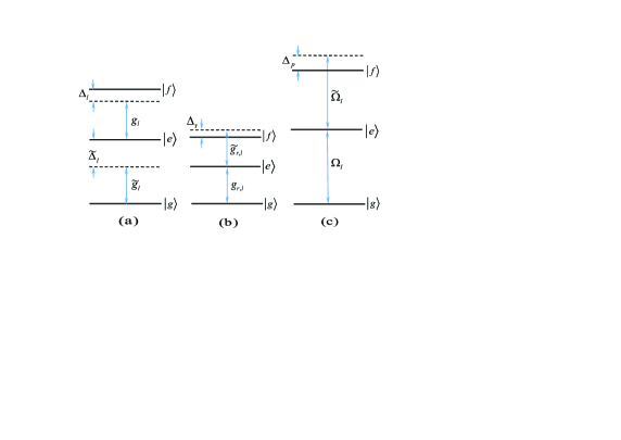
Figure 5: (color online) (a) Dispersive interaction between cavity $l$ and the $\left|e\right\rangle$ $\leftrightarrow$ $\left|f\right\rangle$ transition of qutrits $\left\{1_{l},2_{l}\right\}$ with coupling strength $g_{l}$ and detuning $\Delta_{l}=\omega_{fe}-\omega_{c_{l}}>0$, as well as the unwanted off-resonant interaction between cavity $l$ and the $\left|g\right\rangle$ $\leftrightarrow$ $\left|e\right\rangle$ transition of qutrits $\left\{1_{l},2_{l}\right\}$ with coupling strength $\widetilde{g}_{l}$ and detuning $\widetilde{\Delta}_{l}=\omega_{eg}-\omega_{c_{l}}>0$. (b) Resonant interaction between cavity $l$ and the $\left|g\right\rangle\leftrightarrow\left|e\right\rangle$ transition of qutrit $3_{l}$ with coupling constant $g_{r,l}$, as well as the unwanted off-resonant interaction between cavity $l$ and the $\left|e\right\rangle\leftrightarrow\left|f\right\rangle$ transition of qutrit $3_{l}$ with coupling constant $\widetilde{g}_{r,l}$ and detuning $\Delta_{r,l}$. (c) Resonant interaction between a classical pulse and the $\left|g\right\rangle\leftrightarrow\left|e\right\rangle$ transition of qutrits $\left\{1_{l},2_{l}\right\}$ with Rabi frequency $\Omega_{l}$, as well as the unwanted off-resonant interaction between the pulse and the $\left|e\right\rangle\leftrightarrow\left|f\right\rangle$ transition of qutrits $\left\{1_{l},2_{l}\right\}$ with Rabi frequency $\widetilde{\Omega}_{l}$ and detuning $\Delta_{p}=\omega_{fe}-\omega_{p}$. Here, $\omega_{p}$ is the pulse frequency.

From the description given in the previous section, one can see that three basic interactions are used in the preparation of the GHZ states, i.e., the three basic interactions described by the Hamiltonians $H_{1},H_{2},$ and $H_{3}$ described above. With the unwanted interaction and the inter-cavity crosstalk being considered, these Hamiltonians are modified as follows:

(i) $H_{1}^{\prime}=H_{1}+\delta\!H_{1}+\varepsilon$, where $\delta\!H_{1}$ describes the unwanted interaction of cavity $l$ with the $\left|g\right\rangle\leftrightarrow\left|e\right\rangle$ transition of qutrits $\left\{1_{l},2_{l}\right\}$ in cavity $l$ ($l=1,2,3,4$) [Fig. 5(a)]. The expression of $\delta\!H_{1}$ is given by

$$\delta H_{1}=\sum\limits_{l=1}^{4}\widetilde{g}_{l}e^{i\widetilde{\Delta}_{l}t}\hat{a}_{l}S_{eg,l}^{+}+\text{H.c.,}$$ (17)

where $S_{eg,l}^{+}=\sum\limits_{j=1}^{2}\left|e\right\rangle_{j_{l}}\left\langle g\right|$, $\widetilde{g}_{l}$ is the coupling strength between cavity $l$ and the $\left|g\right\rangle\leftrightarrow\left|e\right\rangle$ transition of qutrits $\left\{1_{l},2_{l}\right\}$, and $\widetilde{\Delta}_{l}=\omega_{eg}-\omega_{c_{l}}$ is the detuning between the frequency of cavity $l$ and the $\left|g\right\rangle\leftrightarrow\left|e\right\rangle$ transition frequency of qutrits $\left\{1_{l},2_{l}\right\}$. In addition, $\varepsilon$ describes the inter-cavity crosstalk between the adjacent cavities, which is given by

$$\varepsilon=g_{12}e^{i\Delta_{12}t}\hat{a}_{1}^{+}\hat{a}_{2}+g_{23}e^{i\Delta_{23}t}\hat{a}_{2}^{+}\hat{a}_{3}+g_{34}e^{i\Delta_{34}t}\hat{a}_{3}^{+}\hat{a}_{4}+\text{H.c.},$$ (18)

where $\Delta_{j(j+1)}=\omega_{c_{j}}-\omega_{c_{j+1}}=\Delta_{j+1}-\Delta_{j}$ $(j=1,2,3)$, $g_{j(j+1)}$ is the crosstalk strength between the two neighbor cavities $j$ and $j+1$ $(j=1,2,3).$ Note that when compared to the crosstalk between the adjacent cavities, the crosstalk between non-adjacent cavities (i.e., cavities $1$ and $3$, cavities $1$ and $4$, and cavities $2$ and $4$) are negligible.

(ii) $H_{2}^{\prime}=H_{2}+\delta\!H_{2}+\varepsilon,$ where $\delta\!H_{2}$ describes the unwanted interaction between cavity $l$ and the $\left|e\right\rangle\leftrightarrow\left|f\right\rangle$ transition of qutrit $3_{l}$ in cavity $l$ ($l=1,2,3,4$) [Fig. 5(b)]. The expression of $\delta\!H_{2}$ is given by

$$\delta\!H_{2}=\widetilde{g}_{r,l}e^{i\Delta_{r,l}t}\hat{a}_{l}\left|f\right\rangle_{3_{l}}\left\langle e\right|+\text{H.c.}$$ (19)

where $\widetilde{g}_{r}$ is the off-resonant coupling strength between cavity $l$ and the $\left|e\right\rangle\leftrightarrow\left|f\right\rangle$ transition of qutrit $3_{l}$ in cavity $l,$ and $\Delta_{r,l}=\omega_{fe}-\omega_{c_{l}}$ is the detuning between the frequency of cavity $l$ and the $\left|e\right\rangle\leftrightarrow\left|f\right\rangle$ transition frequency of qutrit $3_{l}.$

(iii) $\widetilde{H}_{3}=H_{3}+\delta\!H_{3}+\varepsilon,$ where $\delta\!H_{3}$ describes the unwanted interaction between the pulse and the $\left|e\right\rangle\leftrightarrow\left|f\right\rangle$ transition of $\left\{1_{l},2_{l}\right\}$ ($l=1,2,3,4$) [Fig. 5(c)]. The expression of $\delta\!H_{3}$ is given by

$$\delta\!H_{3}=\widetilde{\Omega}_{l}e^{-i\phi}e^{-i\Delta_{p}t}S_{fe,l}^{+}+\text{H.c.}$$ (20)

where $S_{fe,l}^{+}=\sum\limits_{j=1}^{2}\left|f\right\rangle_{j_{l}}\left\langle e\right|,$ $\widetilde{\Omega}_{l}$ is the pulse Rabi frequency associated with the $\left|e\right\rangle\leftrightarrow\left|f\right\rangle$ transition of the qutrits, and $\Delta_{p}=\omega_{fe}-\omega_{p}=\omega_{fe}-\omega_{eg}$ is the detuning between the pulse frequency $\omega_{p}$ and the $\left|e\right\rangle\leftrightarrow\left|f\right\rangle$ transition frequency of the qutrits.

It should be mentioned that the $\left|g\right\rangle\leftrightarrow\left|f\right\rangle$ transition induced by the pulse or the cavities is negligible because $\omega_{eg},\omega_{fe}\ll\omega_{fg}$ (Fig. 2). For simplicity, we also assume that the effect of the qutrit decoherence and the cavity decay during the adjustment of the qutrit level spacings is negligible because for transmon qutrits the level spacings can be rapidly adjusted.

After taking into account the qutrit decoherence and the cavity decay, the system dynamics, under the Markovian approximation, is determined by the master equation

$$\frac{d\rho}{dt} = -i\left[H_{k}^{\prime},\rho\right]+\sum\limits_{l=1}^{4}\kappa_{l}\mathcal{L}\left[\hat{a}_{l}\right]+$$ (21)

$$+\gamma_{eg}\sum\limits_{l=1}^{4}\sum\limits_{j=1}^{3}\mathcal{L}\left[\sigma_{eg,j_{l}}^{-}\right]+\gamma_{fe}\sum\limits_{l=1}^{4}\sum\limits_{j=1}^{3}\mathcal{L}\left[\sigma_{fe,j_{l}}^{-}\right]+\gamma_{fg}\sum\limits_{l=1}^{4}\sum\limits_{j=1}^{3}\mathcal{L}\left[\sigma_{fg,j_{l}}^{-}\right]$$

$$+\gamma_{\varphi,e}\sum\limits_{l=1}^{4}\sum\limits_{j=1}^{3}\left(\sigma_{ee,j_{l}}\rho\sigma_{ee,j_{l}}-\sigma_{ee,j_{l}}\rho/2-\rho\sigma_{ee,j_{l}}/2\right)$$

$$+\gamma_{\varphi,f}\sum\limits_{l=1}^{4}\sum\limits_{j=1}^{3}\left(\sigma_{ff,j_{l}}\rho\sigma_{ff,j_{l}}-\sigma_{ff,j_{l}}\rho/2-\rho\sigma_{ff,j_{l}}/2\right),$$

where $H_{k}^{\prime}$ (with $k=1,2,3$) are the modified Hamiltonians $H_{1}^{\prime},$ $H_{2}^{\prime},$ and $H_{3}^{\prime}$ given above, $\mathcal{L}\left[\Lambda\right]=\Lambda\rho\Lambda^{+}-\Lambda^{+}\Lambda\rho/2-\rho\Lambda^{+}\Lambda/2$ (with $\Lambda=\hat{a}_{l},,\sigma_{fe,j_{l}}^{-},\sigma_{eg,j_{l}}^{-},\sigma_{fg,j_{l}}^{-}$), $\sigma_{fe,j_{l}}^{-}=\left|e\right\rangle_{j_{l}}\left\langle f\right|,$ $\sigma_{eg,j_{l}}^{-}=\left|g\right\rangle_{j_{l}}\left\langle e\right|,$ $\sigma_{fg,j_{l}}^{-}=\left|g\right\rangle_{j_{l}}\left\langle f\right|,$ $\sigma_{ee,j_{l}}=\left|e\right\rangle_{j_{l}}\left\langle e\right|$, and $\sigma_{ff,j_{l}}=\left|f\right\rangle_{j_{l}}\left\langle f\right|.$ In addition, $\kappa_{l}$ is the decay rate of cavity $l$; $\gamma_{eg}$ is the energy relaxation rate for the level $\left|e\right\rangle$ associated with the decay path $\left|e\right\rangle\rightarrow\left|g\right\rangle$; $\gamma_{fe}$ ($\gamma_{fg}$) is the relaxation rate for the level $\left|f\right\rangle$ related to the decay path $\left|f\right\rangle\rightarrow\left|e\right\rangle$ ($\left|f\right\rangle\rightarrow\left|g\right\rangle$); $\gamma_{\varphi,e}$ ($\gamma_{\varphi,f}$) is the dephasing rate of the level $\left|e\right\rangle$ ($\left|f\right\rangle$).

The fidelity of the operation is given by $\mathcal{F}=\sqrt{\left\langle\psi_{id}\right|\rho\left|\psi_{id}\right\rangle},$ where $\left|\psi_{id}\right\rangle$ is the ideal output state given by

$$\frac{1}{\sqrt{2}}\left(\prod\limits_{j=1}^{3}\left|g\right\rangle_{j_{1}}\prod\limits_{j=1}^{3}\left|g\right\rangle_{j_{2}}\prod\limits_{j=1}^{3}\left|e\right\rangle_{j_{3}}\prod\limits_{j=1}^{3}\left|e\right\rangle_{j_{4}}+\prod\limits_{j=1}^{3}\left|e\right\rangle_{j_{1}}\prod\limits_{j=1}^{3}\left|e\right\rangle_{j_{2}}\prod\limits_{j=1}^{3}\left|g\right\rangle_{j_{3}}\prod\limits_{j=1}^{m}\left|g\right\rangle_{j_{4}}\right)\otimes\prod\limits_{l=1}^{4}\left|0\right\rangle_{c_{l}},$$ (22)

when the four TLRs are initially in the GHZ state $\frac{1}{\sqrt{2}}\left(\left|0\right\rangle_{c_{1}}\left|0\right\rangle_{c_{2}}\left|1\right\rangle_{c_{3}}\left|1\right\rangle_{c_{4}}+\left|1\right\rangle_{c_{1}}\left|1\right\rangle_{c_{2}}\left|0\right\rangle_{c_{3}}\left|0\right\rangle_{c_{4}}\right)$ (see the appendix for the details of preparing the four TLRs in this GHZ state), while $\rho$ is the final density matrix obtained by numerically solving the master equation.

We now numerically calculate the fidelity. For a transmon qutrit, the level spacing anharmonicity $100\sim 720$ MHz was reported in experiments [61]. As an example, consider $\Delta_{r,l}/2\pi=\Delta_{p}/2\pi=-\left(\widetilde{\Delta}_{l}-\Delta_{l}\right)/2\pi=-0.7$ GHz. By choosing $\Delta_{1}/2\pi=\Delta_{3}/2\pi=100$ MHz and $\Delta_{2}/2\pi=\Delta_{4}/2\pi=80$ MHz, we have $\Delta_{12}/2\pi=-20$ MHz, $\Delta_{23}/2\pi=20$ MHz, and $\Delta_{34}/2\pi=-20$ MHz. With the choice of $\Delta_{1},\Delta_{2},\Delta_{3},\Delta_{4}$ here, one has $g_{2}=g_{4}=\sqrt{\frac{4}{5}}g_{1}$ and $g_{3}=g_{1}$ according to Eq. (14). For transmon qutrits [62], $\widetilde{g}_{l}=g_{l}/\sqrt{2},$ $\widetilde{g}_{r,l}=\sqrt{2}g_{r,l},$ $\widetilde{\Omega}_{l}=\sqrt{2}\Omega_{l}.$ For simplicity, we assume $g_{r,l}=\widetilde{g}_{l}.$ In addition, we choose $g_{12},g_{23},g_{34}=0.01\max\{g_{1},g_{2},g_{3}\},$ which is achievable in experiments by a prior design of the sample with appropriate capacitances $c_{11},c_{12},c_{22,}c_{23},c_{33},c_{34}$ [63]. Other parameters used in the numerical simulation are: (i) $\gamma_{eg}^{-1}=60$ $\mu$s, $\gamma_{fg}^{-1}=150$ $\mu$s [64], $\gamma_{fe}^{-1}=30$ $\mu$s, $\gamma_{\phi,e}^{-1}=\gamma_{\phi,f}^{-1}=20$ $\mu$s, (ii) $\Omega_{l}/2\pi=45$ MHz. Here, we consider a rather conservative case for decoherence time of the transmon qutrit [65,66]. For simplicity, we assume $\kappa_{l}=\kappa$ in our numerical simulation ($l=1,2,3,4$).

By numerically solving the master equation (21), we plot Fig. 6 for $\kappa^{-1}=10$ $\mu$s, which shows the fidelity versus $g_{1}.$ From Fig. 6, one can see that for $g_{1}/2\pi\sim$ $14.15$ MHz, a high fidelity $\sim 90\%$ can be obtained. For the value of $g_{1}$ here, $g_{2}/2\pi,g_{4}/2\pi\sim 12.65$ MHz; $g_{3}\sim 14.15$ MHz; $g_{r,1}/2\pi,g_{r,3}/2\pi\sim 10$ MHz; and $g_{r,2}/2\pi,g_{r,4}/2\pi=8.95$ MHz, which are readily available in experiments because a coupling strength $g/2\pi$ $\sim 360$ MHz has been reported for a transmon qutrit coupled to a TLR [67,68].

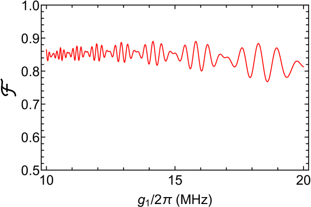
Figure 6: (color online) Fidelity versus $g_{1}$. The parameters used in the numerical simulation are referred to the text

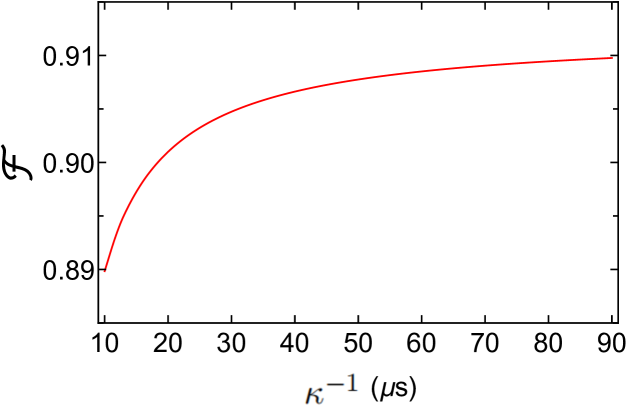
Figure 7: (color online) Fidelity versus $\kappa^{-1}$ for $g_{1}/2\pi=$ $14.15$ MHz and $\Omega_{l}/2\pi=45$ MHz. Other parameters used in the numerical simulation are the same as those used in Fig. 6.

To see how the fidelity changes with the cavity decay rate, we plot Fig. 7, which shows the fidelity versus $\kappa^{-1}$ for $g_{1}/2\pi=$ $14.15$ MHz and $\Omega_{l}/2\pi=45$ MHz. Fig. 7 demonstrates that the fidelity strongly depends on the photon lifetime of the cavities. For $\kappa^{-1}=20$ $\mu$s, a high fidelity $>90\%$ can be achieved. We remark that the fidelity can be further increased by improving the system parameters.

The operation time is $\sim 0.27$ $\mu$s, which is much shorter than the decoherence times of transmon qutrits used in our numerical simulations. For a transmon qutrit, the typical transition frequency between two neighbor levels is $1-20$ GHz. As an example, we consider $\omega_{eg}/2\pi\sim 6.7$ GHz and $\omega_{fe}/2\pi\sim 6.0$ GHz for the case of the transmon qutrits being dispersively coupled to their cavities. Thus, for the values of $\Delta_{1},\Delta_{2},\Delta_{3},\Delta_{4}$ chosen above, one has $\omega_{c_{1}}/2\pi=\omega_{c_{3}}/2\pi=6.6$ GHz and $\omega_{c_{2}}/2\pi=\omega_{c_{4}}/2\pi=6.62$ GHz. For the cavity frequencies here and $\kappa^{-1}=10$ $\mu$s, the quality factors of the four cavities are $Q_{1},Q_{3}\sim 4.14\times 10^{5}$ and $Q_{2},Q_{4}\sim 4.16\times 10^{5}$, which are available because TLRs with a loaded quality factor $Q\sim 10^{6}$ have been experimentally demonstrated [69,70]. The analysis given above shows that high-fidelity creation of GHZ states of four-group SC qubits distributed in four cavities is feasible with the present circuit QED technology.

Further investigation on the experimental feasibility of creating GHZ states of more qubits distributed in different cavities would be necessary. However, we note that the numerical simulations become rather lengthy and complex as the number of qubits increases, which is beyond the scope of this theoretical work.

V. CONCLUSION

We have presented an approach to generate Greenberger-Horne-Zeilinger (GHZ) entangled states of multiple groups of qubits distributed in multiple cavities. From the above description, one can see that as long as the cavities are initially prepared in a GHZ state, all qubits in the cavities can be entangled via a 3-step operation only, no matter what type of architecture the cavity-based quantum network preserves and in which way the cavities are coupled. This proposal also has some additional advantages stated in the introduction. Our numerical simulation shows that high-fidelity preparation of GHZ states of four-group SC qubits, each group containing three qubits and the four groups distributed in four cavities, is feasible with current circuit QED technology. By increasing the number of resonators, GHZ states of more groups of SC qubits distributed in multiple cavities can be created. This work opens a way for quantum state engineering with many qubits distributed in different cavity nodes of a quantum network. We wish that it will stimulate experimental activities in the near future.

As a final note, it should be stressed that this proposal is based on the prerequisite that the cavities are initially prepared in a GHZ state. Nevertheless, this work is of interest, because it may be easy to entangle the cavities when compared to directly entangle a large number of qubits distributed in different cavities without aid of the cavity initial GHZ states and because the proposal works for a 1D, 2D, or 3D quantum network composed of cavities.

ACKNOWLEDGMENTS

This work was partly supported by the Key R$\&$D Program of Guangdong province (2018B030326001), the National Natural Science Foundation of China (NSFC) (11074062, 11374083, 11774076), the NKRDP of China (2016YFA0301802), and the Jiangxi Natural Science Foundation (20192ACBL20051).

APPENDIX: PREPARATION OF THE GHZ STATE OF THE FOUR TLRs

The ladder-type three levels of each of the coupler qutrits ($q_{1},q_{2},q_{3}$) in Fig. 4 are labeled as $\left|g\right\rangle,$ $\left|e\right\rangle,$ and $\left|f\right\rangle$ with energy $E_{g}<E_{e}<E_{f}.$ Initially, $q_{1}$ is in the state $\left(\left|e\right\rangle+\left|f\right\rangle\right)/\sqrt{2},$ $q_{2}$ and $q_{3}$ are in the ground state $\left|g\right\rangle,$ and each TLR is in a vacuum state. In addition, assume that $q_{1},$ $q_{2}$ and $q_{3}$ are decoupled from their neighbor TLRs. Previously, we have set $\omega_{c_{1}}=\omega_{c_{3}}$ and $\omega_{c_{2}}=\omega_{c_{4}}$ in Fig. 4, i.e., every two neighbor TLRs have different frequencies.

The procedure for preparing the GHZ state $\left(\left|0\right\rangle_{c_{1}}\left|0\right\rangle_{c_{2}}\left|1\right\rangle_{c_{3}}\left|1\right\rangle_{c_{4}}+\left|1\right\rangle_{c_{1}}\left|1\right\rangle_{c_{2}}\left|0\right\rangle_{c_{3}}\left|0\right\rangle_{c_{4}}\right)/\sqrt{2}$ of the four TLRs is listed as follows:

Step 1: Adjust the level spacings of $q_{2}$ such that TLR $2$ is resonant with the $\left|g\right\rangle\leftrightarrow$ $\left|e\right\rangle$ transition of $q_{2},$ with a coupling constant $\mu_{1}.$ After an interaction time $\pi/\left(2\mu_{1}\right)$ (i.e., half a Rabi oscillation), the state $\left|e\right\rangle_{q_{2}}\left|0\right\rangle_{c_{2}}$ changes to $-i\left|g\right\rangle_{q_{2}}\left|1\right\rangle_{c_{2}}.$ Hence, the initial state $\frac{1}{\sqrt{2}}\left(\left|e\right\rangle_{q_{2}}+\left|f\right\rangle_{q_{2}}\right)\left|0\right\rangle_{c_{2}}\left|0\right\rangle_{c_{3}}$ of the system, composed of ($q_{2}$, TLR $2$ and TLR $3$), becomes

$$\frac{1}{\sqrt{2}}\left(-i\left|g\right\rangle_{q_{2}}\left|1\right\rangle_{c_{2}}+\left|f\right\rangle_{q_{2}}\left|0\right\rangle_{c_{2}}\right)\left|0\right\rangle_{c_{3}}.$$ (23)

(In the following, the normalization factor $\frac{1}{\sqrt{2}}$ will be omitted for simplicity). Then, adjust the level spacings of $q_{2}$ such that $q_{2}$ is decoupled from TLR $2.$ Now apply a classical pulse (resonant with the $\left|g\right\rangle\leftrightarrow$ $\left|e\right\rangle$ transition) to $q_{2}$ to pump the state $\left|g\right\rangle$ back to the state $\left|e\right\rangle$. Thus, the state (23) changes to

$$\left(-i\left|e\right\rangle_{q_{2}}\left|1\right\rangle_{c_{2}}+\left|f\right\rangle_{q_{2}}\left|0\right\rangle_{c_{2}}\right)\left|0\right\rangle_{c_{3}}.$$ (24)

Step 2: Adjust the level spacings of $q_{2}$ such that TLR $2$ is resonant with the $\left|g\right\rangle\leftrightarrow$ $\left|e\right\rangle$ transition of $q_{2}$ again. After an interaction time $\pi/\left(2\sqrt{2}\mu_{1}\right)$, we have the transformation $\left|e\right\rangle_{q_{2}}\left|1\right\rangle_{c_{2}}$ $\rightarrow$ $-i\left|g\right\rangle_{q_{2}}\left|2\right\rangle_{c_{2}}$ while the state $\left|f\right\rangle_{q_{2}}\left|0\right\rangle_{c_{2}}$ remains unchanged. Hence, the state (24) becomes

$$\left(-\left|g\right\rangle_{q_{2}}\left|2\right\rangle_{c_{2}}+\left|f\right\rangle_{q_{2}}\left|0\right\rangle_{c_{2}}\right)\left|0\right\rangle_{c_{3}}.$$ (25)

Then, adjust the level spacings of $q_{2}$ such that $q_{2}$ is decoupled from TLR $2.$

Step 3: Adjust the level spacings of $q_{2}$ such that TLR $3$ is resonant with the $\left|e\right\rangle\leftrightarrow$ $\left|f\right\rangle$ transition of $q_{2},$ with a coupling constant $\mu_{2}.$ After an interaction time $\pi/\left(2\mu_{2}\right)$, the state $\left|f\right\rangle_{q_{2}}\left|0\right\rangle_{c_{3}}$ changes to $-i\left|e\right\rangle_{q_{2}}\left|1\right\rangle_{c_{3}}.$ Thus, the state (25) becomes

$$\left|g\right\rangle_{q_{2}}\left|2\right\rangle_{c_{2}}\left|0\right\rangle_{c_{3}}+i\left|e\right\rangle_{q_{2}}\left|0\right\rangle_{c_{2}}\left|1\right\rangle_{c_{3}}.$$ (26)

Then, adjust the level spacings of $q_{2}$ such that $q_{2}$ is decoupled from TLR $3.$ Now apply a classical pulse (resonant with the $\left|e\right\rangle\leftrightarrow\left|f\right\rangle$ transition) to $q_{2}$ to pump the state $\left|e\right\rangle$ back to the state $\left|f\right\rangle$. Thus, the state (26) changes to

$$\left|g\right\rangle_{q_{2}}\left|2\right\rangle_{c_{2}}\left|0\right\rangle_{c_{3}}+i\left|f\right\rangle_{q_{2}}\left|0\right\rangle_{c_{2}}\left|1\right\rangle_{c_{3}}.$$ (27)

Step 4: Apply a classical pulse (resonant with the $\left|g\right\rangle\leftrightarrow$ $\left|e\right\rangle$ transition) to $q_{2}$ to pump the state $\left|g\right\rangle$ to the state $\left|e\right\rangle$. Thus, the state (27) changes to

$$\left|e\right\rangle_{q_{2}}\left|2\right\rangle_{c_{2}}\left|0\right\rangle_{c_{3}}+i\left|f\right\rangle_{q_{2}}\left|0\right\rangle_{c_{2}}\left|1\right\rangle_{c_{3}}.$$ (28)

Then, adjust the level spacings of $q_{2}$ such that TLR $3$ is resonant with the $\left|e\right\rangle\leftrightarrow$ $\left|f\right\rangle$ transition of $q_{2}$ again. After an interaction time $\pi/\left(2\sqrt{2}\mu_{2}\right)$, one has the transformation $\left|f\right\rangle_{q_{2}}\left|1\right\rangle_{c_{3}}$ $\rightarrow$ $-i\left|e\right\rangle_{q_{2}}\left|2\right\rangle_{c_{3}}$ while the state $\left|e\right\rangle_{q_{2}}\left|0\right\rangle_{c_{3}}$ remains unchanged. Thus, the state (28) changes to

$$\left(\left|2\right\rangle_{c_{2}}\left|0\right\rangle_{c_{3}}+\left|0\right\rangle_{c_{2}}\left|2\right\rangle_{c_{3}}\right)\left|e\right\rangle_{q_{2}}.$$ (29)

The, adjust the level spacings of $q_{2}$ such that $q_{2}$ is decoupled from TLR $3.$

From the description given above, one can see that TLR $2$ is decoupled from $q_{2}$ during the operation of steps (3) and (4). In addition, it is noted that the initial states of TLRs {$1,4\}$ and coupler qutrits {$q_{1},q_{3}\}$ in Fig. 4 remain unchanged because they are not involved during each operation of steps $(1)-(4)$ above. Thus, based on Eq. (29), the state of the whole system after the above 4-step operation is

$$\left(\left|2\right\rangle_{c_{2}}\left|0\right\rangle_{c_{3}}+\left|0\right\rangle_{c_{2}}\left|2\right\rangle_{c_{3}}\right)\left|e\right\rangle_{q_{2}}\left|g\right\rangle_{q_{1}}\left|g\right\rangle_{q_{3}}\left|0\right\rangle_{c_{1}}\left|0\right\rangle_{c_{4}}.$$ (30)

The purpose of the remaining operations, described below, is to transfer one photon from TLR $2$ to TLR $1$ via $q_{1}$ and one photon from TLR $3$ to TLR $4$ via $q_{3}.$

Step 5: Adjust the level spacings of $q_{1}$ such that TLR $2$ is resonant with the $\left|g\right\rangle\leftrightarrow$ $\left|e\right\rangle$ transition of $q_{1},$with a coupling constant $\mu_{3}$ After an interaction time $\pi/\left(2\sqrt{2}\mu_{3}\right)$, the state $\left|g\right\rangle_{q_{1}}\left|2\right\rangle_{c_{2}}$ $\rightarrow$ $-i\left|e\right\rangle_{q_{1}}\left|1\right\rangle_{c_{2}}$ while the state $\left|g\right\rangle_{q_{1}}\left|0\right\rangle_{c_{2}}$ remains unchanged. Thus, the state (30) becomes

$$\left(-i\left|1\right\rangle_{c_{2}}\left|0\right\rangle_{c_{3}}\left|e\right\rangle_{q_{1}}+\left|0\right\rangle_{c_{2}}\left|2\right\rangle_{c_{3}}\left|g\right\rangle_{q_{1}}\right)\left|e\right\rangle_{q_{2}}\left|g\right\rangle_{q_{3}}\left|0\right\rangle_{c_{1}}\left|0\right\rangle_{c_{4}}.$$ (31)

Then, adjust the level spacings of $q_{1}$ such that TLR $2$ is decoupled from $q_{1}$ but TLR $1$ is resonant with the $\left|g\right\rangle\leftrightarrow$ $\left|e\right\rangle$ transition of $q_{1},$ with a coupling constant $\mu_{4}.$ After an interaction time $\pi/\left(2\mu_{4}\right),$ we have the transformation $\left|e\right\rangle_{q_{1}}\left|0\right\rangle_{c_{1}}$ $\rightarrow$ $-i\left|g\right\rangle_{q_{1}}\left|1\right\rangle_{c_{1}}$ while the state $\left|g\right\rangle_{q_{1}}\left|0\right\rangle_{c_{1}}$ remains unchanged. Hence, the state (31) changes to

$$\left(-\left|1\right\rangle_{c_{1}}\left|1\right\rangle_{c_{2}}\left|0\right\rangle_{c_{3}}+\left|0\right\rangle_{c_{1}}\left|0\right\rangle_{c_{2}}\left|2\right\rangle_{c_{3}}\right)\left|g\right\rangle_{q_{1}}\left|e\right\rangle_{q_{2}}\left|g\right\rangle_{q_{3}}\left|0\right\rangle_{c_{4}}.$$ (32)

Then, adjust the level spacings of $q_{1}$ such that both TLRs $1$ and $2$ are decoupled from $q_{1}.$

Step 6: Adjust the level spacings of $q_{3}$ such that TLR $3$ is resonant with the $\left|g\right\rangle\leftrightarrow$ $\left|e\right\rangle$ transition of $q_{3},$ with a coupling constant $\mu_{5}$. After an interaction time $\pi/\left(2\sqrt{2}\mu_{5}\right)$, the state $\left|g\right\rangle_{q_{3}}\left|2\right\rangle_{c_{3}}$ $\rightarrow$ $-i\left|e\right\rangle_{q_{3}}\left|1\right\rangle_{c_{3}}$ while the state $\left|g\right\rangle_{q_{3}}\left|0\right\rangle_{c_{3}}$ remains unchanged. Thus, the state (32) becomes

$$\left(\left|1\right\rangle_{c_{1}}\left|1\right\rangle_{c_{2}}\left|0\right\rangle_{c_{3}}\left|g\right\rangle_{q_{3}}+i\left|0\right\rangle_{c_{1}}\left|0\right\rangle_{c_{2}}\left|1\right\rangle_{c_{3}}\left|e\right\rangle_{q_{3}}\right)\left|g\right\rangle_{q_{1}}\left|e\right\rangle_{q_{2}}\left|0\right\rangle_{c_{4}}.$$ (33)

Then, adjust the level spacings of $q_{3}$ such that TLR $3$ is decoupled from $q_{3}$ but TLR $4$ is resonant with the $\left|g\right\rangle\leftrightarrow$ $\left|e\right\rangle$ transition of $q_{3},$ with a coupling constant $\mu_{6}.$ After an interaction time $\pi/\left(2\mu_{6}\right),$ we have the transformation $\left|e\right\rangle_{q_{3}}\left|0\right\rangle_{c_{4}}$ $\rightarrow$ $-i\left|g\right\rangle_{q_{3}}\left|1\right\rangle_{c_{4}}$ while the state $\left|g\right\rangle_{q_{3}}\left|0\right\rangle_{c_{4}}$ remains unchanged. Therefore, the state (33) becomes

$$\left(\left|1\right\rangle_{c_{1}}\left|1\right\rangle_{c_{2}}\left|0\right\rangle_{c_{3}}\left|0\right\rangle_{c_{4}}+\left|0\right\rangle_{c_{1}}\left|0\right\rangle_{c_{2}}\left|1\right\rangle_{c_{3}}\left|1\right\rangle_{c_{4}}\right)\left|g\right\rangle_{q_{1}}\left|e\right\rangle_{q_{2}}\left|g\right\rangle_{q_{3}}.$$ (34)

Then, adjust the level spacings of $q_{3}$ such that both TLRs $3$ and $4$ are decoupled from $q_{3}.$ Eq. (34) shows that the four TLRs are prepared in the GHZ state $\left(\left|0\right\rangle_{c_{1}}\left|0\right\rangle_{c_{2}}\left|1\right\rangle_{c_{3}}\left|1\right\rangle_{c_{4}}+\left|1\right\rangle_{c_{1}}\left|1\right\rangle_{c_{2}}\left|0\right\rangle_{c_{3}}\left|0\right\rangle_{c_{4}}\right)/\sqrt{2},$ while the three coupler qutrits ($q_{1},q_{2},q_{3}$) are disentangled from the four TLRs.

Since each step of operation employs the resonant qutrit-cavity or qutrit-pulse interaction, the GHZ state of the four TLRs can be fast prepared within a short time.

References

(1) S. Seidelin, J. Chiaverini, R. Reichle, J. J. Bollinger, D.
Leibfried, J. Britton, J. H. Wesenberg, R. B. Blakestad, R. J. Epstein, D.
B. Hume, W. M. Itano, J. D. Jost, C. Langer, R. Ozeri, N. Shiga, and D. J.
Wineland, Microfabricated surface-electrode ion trap for scalable quantum
information processing, Phys. Rev. Lett. 96, 253003 (2006).
(2) K. Nemoto, M. Trupke, S. J. Devitt, A. M. Stephens, B.
Scharfenberger, K. Buczak, T. Nöbauer, M. S. Everitt, J. Schmiedmayer,
and W. J. Munro, Photonic Architecture for Scalable Quantum Information
Processing in Diamond, Phys. Rev. X 4, 031022 (2014).
(3) X. Qiang, X. Zhou, J. Wang, C. M. Wilkes, T. Loke, S. O’Gara,
L. Kling, G. D. Marshall, R. Santagati, T. C. Ralph, J. B. Wang, J. L.
O’Brien, M. G. Thompson, and J. C. F. Matthews, Large-scale silicon quantum
photonics implementing arbitrary two-qubit processing, Nature Photonics
12, 534 (2018).
(4) C. P. Yang, Q. P. Su, S. B. Zheng, and S. Han, Generating
entanglement between microwave photons and qubits in multiple cavities
coupled by a superconducting qutrit, Phys. Rev. A 87, 022320 (2013).
(5) M. Mariantoni, F. Deppe, A. Marx, R. Gross, F. K. Wilhelm, and
E. Solano, Two-resonator circuit quantum electrodynamics: A superconducting
quantum switch, Phys. Rev. B 78, 104508 (2008).
(6) M. A. Nielsen and I. L. Chuang, Quantum Computation and
Quantum Information (Cambridge University Press, Cambridge, England, 2001).
(7) P. W. Shor, in Proceedings of the 35th Annual Symposium
on Foundations of Computer Science (IEEE Computer Society Press, Santa Fe,
NM, 1994).
(8) M. Hillery, V. Buzék, and A. Berthiaume, Quantum secret
sharing, Phys. Rev. A 59, 1829 (1999).
(9) S. Bose, V. Vedral, and P. L. Knight, Multiparticle
generalization of entanglement swapping, Phys. Rev. A 57, 822
(1998).
(10) R. Cleve, D. Gottesman, and H. K. Lo, How to Share a Quantum
Secret, Phys. Rev. Lett. 83, 648 (1999).
(11) C. P. Yang, Shih I. Chu, and S. Han, Efficient many-party
controlled teleportation of multiqubit quantum, Phys. Rev. A 70,
022329 (2004).
(12) D. P. DiVincenzo and P. W. Shor, Fault-Tolerant Error
Correction with Efficient Quantum Codes, Phys. Rev. Lett. 77, 3260
(1996).
(13) J. Preskill, Reliable quantum computers, Proc. R. Soc. London
A 454, 385 (1998).
(14) V. Giovannetti, S. Lloyd, and L. Maccone, Quantum-enhanced
measurements: Beating the standard quantum Limit, Science 306, 1330
(2004).
(15) J. J. Bollinger, W. M. Itano, D. J. Wineland, and D. J.
Heinzen, Optimal frequency measurements with maximally correlated states,
Phys. Rev. A 54, 4649 (1996).
(16) S. F. Huelga, C. Macchiavello, T. Pellizzari, A. K. Ekert, M.
B. Plenio, and J. I. Cirac, Improvement of frequency standards with quantum
entanglement, Phys. Rev. Lett. 79, 3865 (1997).
(17) T. Monz, P. Schindler, J. T. Barreiro, M. Chwalla, D. Nigg, W.
A. Coish, M. Harlander, W. Hansel, M. Hennrich, and R. Blatt, 14-Qubit
Entanglement: Creation and Coherence, Phys. Rev. Lett. 106, 130506
(2011).
(18) A. Omran, H. Levine, A. Keesling, G. Semeghini, T. T. Wang, S.
Ebadi, H. Bernien, A. S. Zibrov, H. Pichler, S. Choi et al.,
Generation and manipulation of Schrödinger cat states in Rydberg atom
arrays, Science 365, 570 (2019).
(19) H. S. Zhong, Y. Li, W. Li, L. C. Peng, Z. E. Su, Y. Hu, Y. M.
He, X. Ding, W. J. Zhang, Hao Li, et al., 12-photon entanglement and
scalable scattershot boson sampling with optimal entangled-photon pairs from
parametric down-conversion, Phys. Rev. Lett. 121, 250505 (2018).
(20) X.-L. Wang, Y.-H. Luo, H.-L. Huang, M.-C. Chen, Z.-E. Su, C.
Liu, C. Chen, W. Li, Y.-Q. Fang, X. Jiang, et al., 18-qubit entanglement
with six Photons’ three degrees of freedom, Phys. Rev. Lett. 120,
260502 (2018).
(21) C. Song, K. Xu, W. Liu, C.-p. Yang, S.-B. Zheng, H. Deng, Q.
Xie, K. Huang, Q. Guo, L. Zhang, et al., 10-qubit entanglement and parallel
logic operations with a superconducting circuit, Phys. Rev. Lett. 119, 180511 (2017).
(22) C. Song, K. Xu, H. Li, Y. Zhang, X. Zhang, W. Liu, Q. Guo, Z.
Wang, W. Ren, J. Hao, H. Feng, H. Fan, D. Zheng, D. Wang, H. Wang, and S.
Zhu, Observation of multi-component atomic Schrödinger cat states of up
to 20 qubits, Science 365, 574 (2019).
(23) J. I. Cirac and P. Zoller, Preparation of macroscopic
superpositions in many-atom systems, Phys. Rev. A 50, R2799 (1994).
(24) C. C. Gerry, Preparation of multiatom entangled states through
dispersive atom–cavity-field interactions, Phys. Rev. A 53, 2857
(1996).
(25) S. B. Zheng, One-Step Synthesis of Multiatom