Symmetry breaking of spatial Kerr solitons in fractional dimension

Abstract

We study symmetry breaking of solitons in the framework of a nonlinear fractional Schrödinger equation (NLFSE), characterized by its Lévy index, with cubic nonlinearity and a symmetric double-well potential. Asymmetric, symmetric, and antisymmetric soliton solutions are found, with stable asymmetric soliton solutions emerging from unstable symmetric and antisymmetric ones by way of symmetry-breaking bifurcations. Two different bifurcation scenarios are possible. First, symmetric soliton solutions undergo a symmetry-breaking bifurcation of the pitchfork type, which gives rise to a branch of asymmetric solitons, under the action of the self-focusing nonlinearity. Second, a family of asymmetric solutions branches off from antisymmetric states in the case of self-defocusing nonlinearity through a bifurcation of an inverted-pitchfork type. Systematic numerical analysis demonstrates that increase of the Lévy index leads to shrinkage or expansion of the symmetry-breaking region, depending on parameters of the double-well potential. Stability of the soliton solutions is explored following the variation of the Lévy index, and the results are confirmed by direct numerical simulations.

I Introduction

Spontaneous symmetry breaking (SSB), i.e., self-organized transformation of symmetric or antisymmetric states into asymmetric ones, is a ubiquitous phenomenon that occurs in a wide variety of intrinsically symmetric physical systems. Examples of the SSB have been investigated theoretically in nonlinear optics SSB-Review-Malomed , Bose-Einstein condensates (BECs) SSB1 ; SSB2 ; SSB3 ; SSB4 , lasers SSB5 , liquid crystals SSB6 , and other areas. In optics, the SSB has been observed, in particular, in a CS₂ planar optical waveguide SSBe1 , in a biased photorefractive crystal (SBN:60) illuminated by a probe beam modulated by an amplitude mask SSBe2 , in symmetrically coupled lasers SSBe3 ; NatPhot2 , metamaterials Kivshar , etc. In BEC, the SSB was reported in the form of macroscopic quantum self-trapping with an imbalanced population, in a condensate of ⁸⁷Rb atoms loaded in a symmetric double-well potential SSBe4 . Especially, as one of fundamental aspects of the optical-soliton phenomenology, the SSB of solitons was intensively investigated in various settings modeled by nonlinear Schrödinger equations (NLSEs) SSB-OptSol1 ; SSB-OptSol2 ; SSB-OptSol3 ; SSB-OptSol4 ; SSB-OptSol5 ; SSB-OptSol6 ; SSB-OptSol7 ; SSB-OptSol8 ; SSB-OptSol9 ; SSB-OptSol10 ; SSB-OptSol11 ; SSB-OptSol12 ; SSB-OptSol13 ; SSB-OptSol14 ; SSB-OptSol15 ; SSB-OptSol16 ; NatPhot1 ; Elad .

Recently, the investigation of SSB of solitons has been expanded into non-Hermitian optical systems, which are modeled by NLSEs with parity-time ($\mathcal{PT}$) symmetric complex potentials PT1 ; PT2 , where families of stable asymmetric one-dimensional (1D) solitons induced by the SSB have been found for specially designed complex potentials YJK1 ; YJK2 ; nonPT-Li ; YJK3 , as well as under the action of 2D potentials nonPT-2D .

An interesting generalization of the Schrödinger equation, corresponding to fractional-dimensional Hamiltonians, was proposed in Refs. FSE2 -FSE1 . It has been introduced, in the context of the quantum theory, via Feynman path integrals over Lévy-flight trajectories, which leads to the fractional Schrödinger equation (FSE). Although implications of such models are still a matter of debate FSE4 ; FSE5 , some experimental schemes have been proposed for emulating them in condensed-matter settings and optical cavities FSE11 ; FSE12 . A number of intriguing dynamical properties have been predicted in the framework of FSEs, including 1D zigzag propagation FSE13 , diffraction-free beams FSE14 ; FSE15 ; FSE16 ; FSE17 ; FSE18 , beam splitting FSE19 , periodic oscillations of Gaussian beams FSE20 , beam-propagation management FSE21 , optical Bloch oscillations and Zener tunneling FSE22 , resonant mode conversion and Rabi oscillations FSE23 , localization and Anderson delocalization FSE24 , and SSB of $\mathcal{PT}$-symmetric modes in a linear FSE FSE25 .

Naturally, FSEs may be applied to nonlinear-optical settings NLFSE2 ; NLFSE3 . Recent works demonstrate that a variety of fractional optical solitons can be produced by nonlinear FSEs (NLFSEs) NLFSE4 , such as “accessible solitons” NLFSE5 ; NLFSE6 ; NLFSE7 , double-hump solitons and fundamental solitons in $\mathcal{PT}$-symmetric potentials NLFSE8 ; NLFSE9 , gap solitons and surface gap solitons in $\mathcal{PT}$-symmetric photonic lattices NLFSE10 ; NLFSE11 , two-dimensional solitons NLFSE12 , and off-site- and on-site-centered vortex solitons in two-dimensional $\mathcal{PT}$-symmetric lattices NLFSE13 . Composition relations between nonlinear Bloch waves and gap solitons have also been addressed in the framework of NLFSE with photonic lattices NLFSE14 , bright solitons under the action of periodically spatially modulated Kerr nonlinearity NLFSE15 , as well as dissipative surface NLFSE16 and bulk solitons Yingji .

Once solitons may undergo various forms of SSB in models based on conventional Hermitian and $\mathcal{PT}$-symmetric NLSEs, it is natural to consider the possibility of similar effects to occur in NLFSEs with symmetric double-well potentials. In this work, we address SSB of solitons in NLFSEs with self-focusing and self-defocusing cubic nonlinearities. The model and numerical methods are introduced in Sec. II. Basic numerical results, including the existence of soliton solutions in the fractional dimension, their SSB bifurcations, and results for stability and dynamics of the solitons are reported in Sec. III. The paper is concluded by Sec. IV.

II The model and methods

II.1 The nonlinear fractional Schrödinger equation

We start the analysis by considering beam propagation along the $z$-axis in a waveguide with the Kerr nonlinearity. The balance between the diffraction in the fractional dimension FSE12 , cubic nonlinearity, and modulation of the linear refractive index makes it possible to form solitons. The corresponding model for the light-beam propagation is based on the following equation:

$$i\frac{\partial A}{\partial z}-\frac{1}{2kw_{0}^{2}}\left(-\frac{\partial^{2}}{\partial\xi^{2}}\right)^{\alpha/2}A+\frac{k\left[n\left(x\right)-n_{0}\right]}{n_{0}}A+k_{0}n_{2}\left|A\right|^{2}A=0,$$ (1)

where $A(z,x)$ is the local amplitude of the optical field, and $\xi=x/w_{0}$ is the normalized transverse coordinate, scaled to characteristic width $w_{0}$ of the input beam. The fractional derivative, $(-\partial^{2}/\partial\xi^{2})^{\alpha/2}$, is determined by the Lévy index, which usually takes values $1\leq\alpha\leq 2$ (this point is additionally considered below). Further, $k=k_{0}n_{0}$ is the wavenumber, with $n_{0}$ being the background refractive index, and $k_{0}=2\pi/\lambda$, where $\lambda$ is the optical wavelength. An effective potential is introduced by local modulation, $n(x)$, of the linear refractive index, while $n_{2}$ is the nonlinear Kerr coefficient of the material.

Equation (1) can be cast in a normalized form by means of additional rescaling, $\Psi(\zeta,\xi)\equiv\left(k_{0}\left|n_{2}\right|L_{d}\right)^{1/2}A(z,x)$, where $L_{d}=kw_{0}^{2}$ is the diffraction length, $\zeta=z/L_{d}$ is the normalized coordinate in the propagating direction, and the effective potential is defined as $-V(\xi)\equiv-L_{d}k\left[n\left(w_{0}\xi\right)-n_{0}\right]/n_{0}$. The scaled equation is

$$i\frac{\partial\Psi}{\partial\zeta}-\frac{1}{2}\left(-\frac{\partial^{2}}{\partial\xi^{2}}\right)^{\alpha/2}\Psi+V\left(\xi\right)\Psi+\sigma\left|\Psi\right|^{2}\Psi=0,$$ (2)

where $\sigma\equiv n_{2}/\left|n_{2}\right|=\pm 1$ corresponds to the self-focusing $(+)$ and defocusing $(-)$ nonlinearity, respectively. Obviously, when $\alpha=2$, Eq. (2) amounts to the standard NLSE, and when $\alpha=1$, the fractional derivative corresponds to the operator in the form of the “square root of Laplacian”, which was introduced long ago in a phenomenological model of instability of combustion fronts Aldushin .

In this paper, we study SSB for soliton solutions to Eq. (2), chiefly with $1\leq\alpha<2$, although the case of $\alpha<1$ is briefly considered too, see Fig. 3 below. To this end, we introduce the effective symmetric double-well potential corresponding to

$$V\left(\xi\right)=V_{0}\left\{\exp\left[-\left(\frac{\xi+\xi_{0}}{W_{0}}\right)^{2}\right]+\exp\left[-\left(\frac{\xi-\xi_{0}}{W_{0}}\right)^{2}\right]\right\},$$ (3)

with potential minima set at points $\xi=\pm\xi_{0}$, while $W_{0}$ and $V_{0}$ denote the width and depth of the local wells.

Soliton solutions produced by Eq. (2) with real propagation constant $\beta$ are sought as

$$\Psi\left(\zeta,\xi\right)=\psi\left(\xi\right)e^{i\beta\zeta},$$ (4)

where the real function $\psi(\xi)$ obeys a stationary equation

$$-\frac{1}{2}\left(-\frac{d^{2}}{d\xi^{2}}\right)^{\alpha/2}\psi+V\left(\xi\right)\psi+\sigma\left|\psi\right|^{2}\psi-\beta\psi=0.$$ (5)

Soliton solutions of Eq. (5) are characterized by the integral power (norm), which is a dynamical invariant of Eq. (2), and may be naturally split in contributions from the left and right regions:

$$P(\beta)\equiv P_{L}(\beta)+P_{R}(\beta)=\int\nolimits_{-\infty}^{+\infty}\left|\Psi\right|^{2}d\xi\equiv\int\nolimits_{-\infty}^{0}\left|\Psi\right|^{2}d\xi+\int\nolimits_{0}^{+\infty}\left|\Psi\right|^{2}d\xi.$$ (6)

Asymmetric states are then characterized by the SSB parameter

$$\Theta=\frac{P_{L}-P_{R}}{P_{L}+P_{R}},$$ (7)

which is used below.

II.2 The numerical method

The fractional derivative in Eq. (5) is defined as a pseudo-differential operator JMP51-062102 ; JMP54-012111

$$\mathcal{F}[\left(-d^{2}/d\xi^{2}\right)^{\alpha/2}\psi]=\left|k\right|^{\alpha}\mathcal{F}\psi(k),$$ (8)

where $\mathcal{F}$ denotes the Fourier transform, which converts functions of $x$ into functions of the respective wavenumber, $k$. Actually, for all values $\alpha<2$, Eq. (5) is a nonlocal equation. Several methods have been developed for handling nonlocal FSEs JCP325 ; CMA71 ; CMA75 .

To obtain numerical soliton solutions of Eq. (5), we employed the Newton-conjugate-gradient method, as presented in Refs. NCG ; Book1 . Accordingly, Eq. (5) is rewritten as

$$L_{0}\psi\left(\xi\right)=0,$$ (9)

where

$$L_{0}=-\frac{1}{2}\left(-\frac{d^{2}}{d\xi^{2}}\right)^{\alpha/2}+V(\xi)+\sigma\left|\psi\right|^{2}-\beta.$$ (10)

Here, the propagation constant $\beta$ is considered as a parameter with a fixed value, while solution $\psi(\xi)$ is generated by means of Newton’s iterations

$$\psi_{n+1}=\psi_{n}+\Delta\psi_{n},$$ (11)

where $\psi_{n}$ is an approximate solution, and correction $\Delta\psi_{n}$ is computed from the linear Newton’s equation

$$L_{1n}\Delta\psi_{n}=-L_{0}\left(\psi_{n}\right),$$ (12)

where $L_{1n}$ is the linearization operator $L_{1}$ corresponding to Eq. (9), evaluated with $\psi$ replaced by approximate solution $\psi_{n}$:

$$L_{1}=-\frac{1}{2}\left(-\frac{d^{2}}{d\xi^{2}}\right)^{\alpha/2}+V+\sigma\left|\psi\right|^{2}+2\sigma\psi\mathtt{Re}\left(\psi^{\ast}\right)-\beta.$$ (13)

In the framework of this scheme, Eq. (12) can be solved directly by dint of conjugate gradient iterations NCG ; Book1 , which yields symmetric, antisymmetric, and asymmetric soliton solutions.

III Numerical results

III.1 Symmetric, antisymmetric, and asymmetric soliton solutions in the fractional dimension

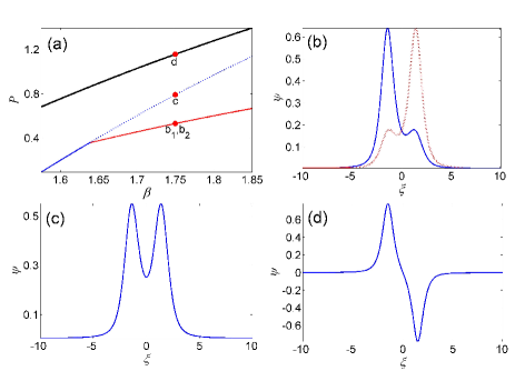
Figure 1: (Color online) SSB of solitons of Eq. (2) with Lévy index $\alpha=1.1$, self-focusing Kerr nonlinearity ($\sigma=+1$), and the double-well potential (3) with parameters $V_{0}=2$, $\xi_{0}=1.5$, and $W_{0}=1.4$. (a) Power curves of families of stable and unstable symmetric solitons (thin solid and dotted blue lines, respectively), stable antisymmetric solitons (the thick solid black line), and stable asymmetric solitons (the thin solid red line). Panels (b), (c), and (d) display asymmetric, symmetric, and antisymmetric soliton solutions at $\beta=1.75$, marked by “b₁,b₂,c,d” in panel (a).

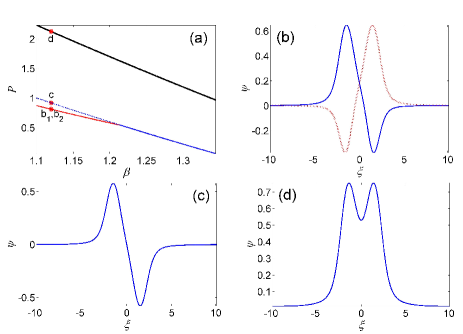
Figure 2: (Color online) SSB of solitons of Eq. (2) with self-defocusing Kerr nonlinearity ($\sigma=-1$), other parameters being the same as in Fig. 1. (a) Power curves of stable symmetric solitons (the thick solid black line), unstable and stable antisymmetric solitons (thin dotted and solid blue lines, respectively), and stable asymmetric solitons (the thin solid red line). Panels (b), (c), and (d) depict asymmetric, antisymmetric, and symmetric solitons at $\beta=1.12$, marked by “b₁,b₂,c,d” in panel (a).

Generic examples of soliton families are presented in Fig. 1. They were found as numerical solutions of Eq. (5) with Lévy index $\alpha=1.1$ and $\sigma=+1$ (the self-focusing sign of the nonlinearity), while the potential $V\left(\xi\right)$ is taken as per Eq. (3) with $V_{0}=2$, $\xi_{0}=1.5$, and $W_{0}=1.4$. Figure 1(a) shows power curves $P(\beta)$ for stable and unstable symmetric-soliton solutions, as well as for stable antisymmetric and stable asymmetric ones in this potential. SSB occurs when the integral power of symmetric solitons exceeds a critical value (which corresponds to the bifurcation point), $P_{\mathrm{cr}}\approx 0.3603$, the respective propagation constant being $\beta_{\mathrm{cr}}\approx 1.6389$. As a result of the SSB, the power curves of the symmetric and asymmetric soliton solutions form a pitchfork bifurcation. As examples, profiles of asymmetric, symmetric, and antisymmetric soliton solutions with $\beta=1.75$ are displayed in Figs. 1(b), 1(c), and 1(d), respectively. Panel 1(b) demonstrates that there actually exist two branches of the asymmetric soliton solutions, which are mirror images of each other, $\psi\left(\xi\right)$ and $\psi\left(-\xi\right)$, represented by coinciding points b₁ and b₂ in Fig. 1(a).

SSB of solitons is also found in Eq. (5) with the self-defocusing nonlinearity ($n_{2}<0$), when the symmetric soliton solutions, shown in Fig. 2(a), are stable, but the antisymmetric ones become unstable at $P_{\mathrm{cr}}\approx 0.5459$ ($\beta_{\mathrm{cr}}\approx 1.2138$) with the increase of the integral power, as is also shown in Fig. 2(a), where a branch of stable asymmetric soliton solutions bifurcates from the branch of the unstable antisymmetric solutions. Figures 2(b), 2(c), and 2(d) display the corresponding profiles of the asymmetric, symmetric, and antisymmetric soliton solutions, respectively, with $\beta=1.12$. In this case too, there are also two branches of asymmetric states, which are mirror images of each other, $\psi(\xi)$ and $\psi(-\xi)$, as can be seen in panel 2(b).

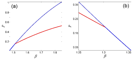
Figure 3: (Color online) SSB of solitons of Eq. (2) with Lévy index $\alpha=0.8$, other parameters being the same as in Fig. 1. (a) Power curves of families of stable and unstable symmetric solitons (solid and dotted blue lines, respectively), and stable asymmetric solitons (the solid red line) with the self-focusing Kerr nonlinearity. (b) Power curves of unstable and stable antisymmetric solitons (dotted and solid blue lines, respectively), and stable asymmetric solitons (the solid red line) with the self-defocusing Kerr nonlinearity.

In fact, even in the case of $\alpha<1$, when solitons, supported by the self-focusing cubic nonlinearity in the free space, are unstable, because of the occurrence of the supercritical collapse Yingji , the trapping potential may stabilize the solitons and uphold the familiar SSB scenario, as shown in Fig. 3(a) for $\alpha=0.8$. In the case of the self-defocusing nonlinearity, values $\alpha<1$ are possible too, giving rise to the same type of SSB as considered above, see Fig. 3(b).

The fact that the growth of the strength of the focusing or defocusing nonlinearity destabilizes, respectively, symmetric or antisymmetric solitons, replacing them by asymmetric ones, is a generic property of SSB SSB-Review-Malomed . It is relevant to mention that, in the latter case, the pitchfork bifurcation may be identified as an inverted one, because it takes place, in Figs. 2(a) and 3(b), with the decrease of the propagation constant (but still with the increase of the integral power). It is also found that, in the case of the self-focusing nonlinearity, the stable soliton branches in Figs. 1(a) and 3(a) satisfy the Vakhitov-Kolokolov (VK) criterion VK1 ; VK2 , and, for the defocusing nonlinearity, the stable soliton solution branches in Figs. 2(a) and 3(b) satisfy the anti-VK criterion anti-VK .

III.2 Symmetry-breaking bifurcations at different values of the Lévy index

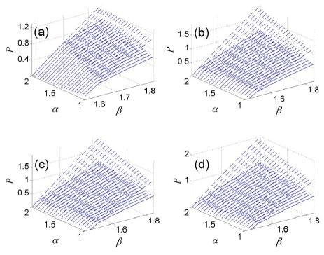
Figure 4: (Color online) The SSB bifurcation represented by dependences of the integral power of unstable and stable symmetric (dashed and solid curves, respectively) and stable asymmetric (solid curves) soliton solutions on Lévy index $\alpha$ and propagation constant $\beta$ in the case of the self-focusing Kerr nonlinearity ($\sigma=+1$) for different values of the separation parameter of the double-well potential (3): (a) $\xi_{0}=1.5$, (b) $\xi_{0}=1.8$, (c) $\xi_{0}=1.9$, and (d) $\xi_{0}=2$, respectively. Other parameters of the potential are the same as in Fig. 1.

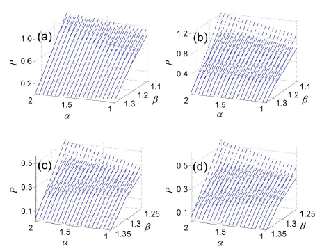
Figure 5: (Color online) The SSB bifurcation represented by dependences of the integral power of unstable and stable antisymmetric (dashed and solid curves, respectively) and stable asymmetric (solid curves) soliton solutions on Lévy index $\alpha$ and propagation constant $\beta$ in the case of the self-defocusing Kerr nonlinearity ($\sigma=-1$) for different values of the separation parameter of the double-well potential (3): (a) $\xi_{0}=1.5$, (b) $\xi_{0}=1.8$, (c) $\xi_{0}=1.9$, and (d) $\xi_{0}=2$, respectively. Other parameters of the potential are the same as in Fig. 1.

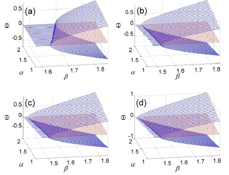
Figure 6: (Color online) SSB bifurcation diagrams shown in terms of asymmetry parameter (7), corresponding to the situation displayed in Fig. 4: (a) $\xi_{0}=1.5$, (b) $\xi_{0}=1.8$, (c) $\xi_{0}=1.9$, and (d) $\xi_{0}=2$. Dashed red curves represent unstable symmetric soliton solutions.

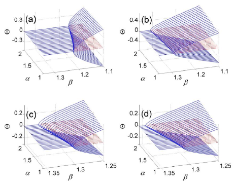
Figure 7: (Color online) SSB bifurcation diagrams shown in terms of asymmetry parameter (7), corresponding to the situation displayed in Fig. 5: (a) $\xi_{0}=1.5$, (b) $\xi_{0}=1.8$, (c) $\xi_{0}=1.9$, and (d) $\xi_{0}=2$. Dashed red curves represent unstable antisymmetric soliton solutions.

To explore how the value of Lévy index $\alpha$ effects the SSB bifurcations, in Figs. 4, 5, 6, 7, 8, and 9, we have produced power curves for soliton families, by numerically solving Eq. (5) and varying $\alpha$ (with interval of $0.05$, in the interval $1\leq\alpha\leq 2$) and separation parameter $\xi_{0}$ of the double-well potential (3). The numerical results for the self-focusing and defocusing cases are summarized in Figs. 4 and 5. Specifically, at $\xi_{0}=1.5$, SSB areas in the plane of $\alpha$ and propagation constant $\beta$ shrink with the increase of $\alpha$, as seen in Fig. 4(a) and 5(a). As $\xi_{0}$ increases to $1.8$, the areas slightly expand with the increase of $\alpha$ in Fig. 4(b) and Fig. 5(b). Then, as $\xi_{0}$ increases to $1.9$ and $2.0$, the SSB areas significantly expand with the increase of $\alpha$ in Figs. 4(c), 4(d), 5(c), and 5(d).

The families of the soliton solutions are further characterized by the dependences of asymmetry parameter (7) on $\alpha$ and $\beta$, which are displayed in Figs. 6 and Figs. 7 for the self-focusing and defocusing nonlinearities, respectively. The results indicate that the SSB bifurcations in Eq. (5) are of the supercritical (alias forward) type, i.e., with branches of asymmetric branches going forward from the bifurcation point book .

Further, Figs. 6 and Figs. 7 clearly demonstrate that the increase of separation $\xi_{0}$ in the double-hump potential (3) shifts the SSB bifurcation to lower values of the power. This conclusion is quite natural, as a larger separation makes the effective linear coupling between the two well weaker, making it easier for the nonlinearity to compete with it SSB-Review-Malomed .

III.3 The linear stability analysis and dynamics

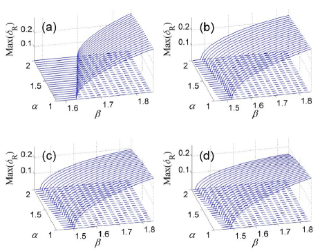
Figure 8: (Color online) Largest linear instability growth rates of symmetric (solid) and asymmetric (dashed) soliton solutions from Fig. 4.

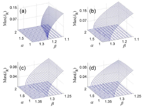
Figure 9: (Color online) Largest linear instability growth rates of antisymmetric (solid) and asymmetric (dashed) soliton solutions in Fig. 5.

Stability of solitons in the present model was explored by considering small perturbations $u\left(\xi\right)$ and $v\left(\xi\right)$ added to a stationary solution, $\psi\left(\xi\right)$, with propagation constant $\beta$, as follows:

$$\Psi\left(\zeta,\xi\right)=e^{i\beta\zeta}\left[\psi\left(\xi\right)+u\left(\xi\right)e^{\delta\zeta}+v^{\ast}\left(\xi\right)e^{\delta^{\ast}\zeta}\right],$$ (14)

where $\delta$ is the instability growth rate (a complex one, in the general case). Substituting this expression in Eq. (2) and linearizing it with respect to the perturbations, we arrive at the following linear eigenvalue problem:

$$i\left(\begin{array}[]{cc}\mathcal{L}_{11}&\mathcal{L}_{12}\\ \mathcal{L}_{21}&\mathcal{L}_{22}\end{array}\right)\left(\begin{array}[]{c}u\\ v\end{array}\right)=\delta\left(\begin{array}[]{c}u\\ v\end{array}\right),$$ (15)

where we define

$$\mathcal{L}_{11}=-\frac{1}{2}\left(-\frac{d^{2}}{d\xi^{2}}\right)^{\alpha/2}+U-\beta+2\sigma\left|\psi\right|^{2},$$ (16)

$$\mathcal{L}_{12}=+\sigma\psi^{2},$$ (17)

$$\mathcal{L}_{21}=-\sigma\psi^{2},$$ (18)

$$\mathcal{L}_{22}=\frac{1}{2}\left(-\frac{d^{2}}{d\xi^{2}}\right)^{\alpha/2}-U+\beta-2\sigma\left|\psi\right|^{2}.$$ (19)

The underlying stationary solution is unstable if the solution of Eq. (15) produces at least one eigenvalue with $\mathrm{Re}(\delta)>0$.

Because Eq. (15) contains the fractional derivative, it is convenient to solve it by means of the Fourier decomposition, which converts the equation into a matrix eigenvalue problem for Fourier coefficients of perturbation eigenfunctions $u\left(\xi\right)$ and $v\left(\xi\right)$. Then, the spectrum can be obtained numerically, using the Fourier collocation and Newton-conjugate-gradient methods Book1 ; Book2 ; Book3 . Both methods have produced identical results.

Figures 8 and 9 display the largest instability growth rates, $\max\left(\delta_{R}\right)$, for symmetric and asymmetric, or antisymmetric and asymmetric, sets of solitons, in the cases of the self-focusing and defocusing nonlinearity, respectively. In agreement with general principles book ; SSB-Review-Malomed , the SSB destabilizes the symmetric or antisymmetric solitons in the former and latter cases, respectively, while the asymmetric solitons remain stable solutions in the entire interval of values of the Lévy index considered in the present work, i.e., $1\leq\alpha\leq 2$.

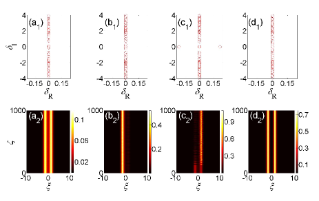
Figure 10: (Color online) The top row: linear-stability spectra for the soliton solutions in the case of the self-focusing nonlinearity, $\sigma=+1$. The bottom row: results of simulations of the perturbed evolution of the solitons from the top row. (a₁,a₂): A stable symmetric soliton with $\beta=1.62$. Panels (b₁,b₂), (c₁,c₂), and (d₁,d₂) display the results for stable asymmetric, unstable symmetric, and stable antisymmetric solitons, respectively, at $\beta=1.75$.

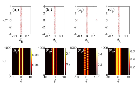
Figure 11: (Color online) The top row: the same as in Fig. 10, but for the self-defocusing nonlinearity, $\sigma=-1$. The bottom row: perturbed evolution of the solitons from the top row. (a₁,a₂): A stable antisymmetric soliton with $\beta=1.3$. Panels (b₁,b₂), (c₁,c₂), and (d₁,d₂) display stable asymmetric, unstable antisymmetric and stable symmetric soliton solutions, respectively, at $\beta=1.12$.

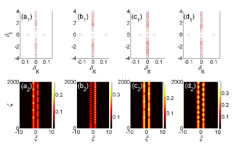
Figure 12: (Color online) The top row: linear-stability spectra for weakly unstable soliton solutions, taken close to the SSB bifurcation points. The bottom row: the perturbed evolution of the solitons from the top row. Panels (a₁,a₂) and (b₁,b₂) display unstable symmetric solitons with $\beta=1.65$ and $1.67$, respectively, in the case of self-focusing. Panels (c₁,c₂) and (d₁,d₂) display unstable antisymmetric solitons with $\beta=1.2$ and $1.17$, respectively, in the case of self-defocusing.

To corroborate predictions of the linear-stability analysis, we have performed numerical simulations of perturbed evolution of the solitons. We start with the self-focusing nonlinearity and display the result for a stable symmetric soliton at $\beta=1.62<\beta_{\mathrm{cr}}=1.6389$. The respective eigenvalue spectrum is shown in Fig. 10(a₁), and the nonlinear evolution under the action of random-noise initial perturbations with a relative amplitude of $10\%$ is presented in Fig. 10(a₂). It is seen that, at least up to $\zeta=1000$, the solution indeed remains stable. Next, we address stable asymmetric, unstable symmetric, and stable antisymmetric soliton solutions for $\beta=1.75>\beta_{\mathrm{cr}}=1.6389$ [stationary profiles of these solutions are shown in Figs. 1(b), 1(c), and 1(d), respectively]. The corresponding linear-stability spectra are shown in top panels of Figs. 10(b₁), 10(c₁), and 10(d₁). The evolution of the stable asymmetric and stable antisymmetric solitons, under the action of random perturbations with the $10\%$ relative amplitude, is displayed in Figs. 10(b₂) and 10(d₂), respectively. On the other hand, Fig. 10(c₂) demonstrates that the symmetric soliton, whose instability is predicted by the spectrum shown in Fig. 10(c₁), quickly develops the instability (even without adding a perturbation to the initial state), and, as it might be expected, the instability tends to convert it into a stable asymmetric state.

In Fig. 11, we display the evolution of the soliton solutions in the case of the self-defocusing nonlinearity, where an antisymmetric soliton at $\beta=1.3>\beta_{\mathrm{cr}}=1.2138$, which is predicted to be stable by Fig. 11(a₁) [$\beta>\beta_{\mathrm{cr}}$ is the stability condition in the case of the self-defocusing nonlinearity, according to Fig. 2(a)], indeed keeps its shape in the course of the perturbed evolution in Fig. 11(a₂). For stable asymmetric, unstable antisymmetric, and stable symmetric solitons, with $\beta=1.12<\beta_{\mathrm{cr}}=1.2138$ [stationary profiles of these solutions are shown in Figs. 2(b), 2(c), and 2(d), respectively], the linear-stability spectra are shown in Figs. 11(b₁), 11(c₁), and 11(d₁), respectively. The perturbed evolution of the solutions, displayed in Figs. 11(b₂) and 11(d₂), corroborates the predicted stability. On the other hand, the unstable antisymmetric soliton develops the instability in the numerical simulations even without addition of perturbations, as seen in Fig. 11(c₂). It is worthy to note that, in this case, the evolution does not tend to convert the unstable soliton into an asymmetric one that would be spontaneously pinned to one potential well; instead, it develops periodic oscillations between the two wells.

We have also considered the evolution of unstable soliton solutions near the bifurcation points, in the cases of both the self-focusing and defocusing signs of the nonlinearity. The results are summarized in Fig. 12. Without the addition of initial perturbations, these unstable solitons develop oscillations, with a period that is larger for a weaker instability [smaller $\max\left(\delta_{R}\right)$]. Thus, the spontaneously emerging oscillations are slower in Figs. 12(a₂) and 12(c₂) than in Figs. 12(b₂) and 12(d₂).

IV Conclusion

We have investigated the phenomenology of SSB (spontaneous symmetry breaking) of spatial Kerr solitons in the model based on the NLFSE (nonlinear fractional Schrödinger equation) with a symmetric double-well potential and self-focusing or defocusing cubic nonlinearity. In agreement with the general principles of the SSB theory, the increase of the soliton’s integral power (norm) destabilizes symmetric and antisymmetric solitons, and creates stable asymmetric ones, in the cases of the self-focusing and self-defocusing nonlinearities, respectively, In either case, stable asymmetric solitons emerge at the SSB bifurcation point, the pitchfork bifurcation always being of the supercritical (forward) type. In the case of the self-defocusing nonlinearity, the bifurcation may be considered as an inverted one, in the sense that it happens with the decrease of the soliton’s propagation constant. The dependence of the SSB effects on the Lévy index, $\alpha$, which characterizes the fractional dimension in the NLFSE, and separation, $\xi_{0}$, between the potential wells in the symmetric potential, has been explored. In particular, the increase of $\alpha$ leads to shrinkage or expansion of the SSB area, depending on the value of $\xi_{0}$.

A relevant direction for the extension of the analysis is to develop it for the study of SSB phenomena in $\mathcal{PT}$-symmetric and dissipative systems.

V Acknowledgments

This work was supported by the National Natural Science Foundation of China (NNSFC) (11805141, 11705108, 11804246), Shanxi Province Science Foundation for Youths (201901D211424), Scientific and Technological Innovation Programs of Higher Education Institutions in Shanxi (STIP) (2019L0782), and Zhejiang Provincial Natural Science Foundation of China (Grant no. LR20A050001). The work of BAM was supported, in a part, by the Israel Science Foundation through grant No. 1287/17.

VI References

References

- (1) Malomed BA. Spontaneous symmetry breaking, self-trapping, and Josephson oscillations. Berlin and Heidelberg: Springer-Verlag; 2013.
- (2) Jackson RK, Weinstein MI. Geometric analysis of bifurcation and symmetry breaking in a Gross-Pitaevskii equation. J Statist Phys 2004;116:881-905.
- (3) Matuszewski M, Malomed BA, Trippenbach M. Spontaneous symmetry breaking of solitons trapped in a double-channel potential. Phys Rev A 2007;75:063621.
- (4) Wang C, Theocharis G, Kevrekidis PG, Whitaker N, Law KJH, Frantzeskakis DJ, Malomed BA. Two-dimensional paradigm for symmetry breaking: The nonlinear Schrödinger equation with a four-well potential. Phys Rev E 2009;80:046611.
- (5) Waclaw B, Sopik J, Janke W, Meyer-Ortmanns H. Tuning the shape of the condensate in spontaneous symmetry breaking. Phys Rev Lett 2009;103:080602.
- (6) Green C, Mindlin GB, D’Angelo EJ, Solari HG, Tredicce JR. Spontaneous symmetry breaking in a laser: the experimental side. Phys Rev Lett 1990;65:3124-3127.
- (7) Vanakaras AG, Photinos DJ, Samulski ET. Tilt, polarity, and spontaneous symmetry breaking in liquid crystals. Phys Rev E 1998;57:R4875.
- (8) Cambournac C, Sylvestre T, Maillotte H, Vanderlinden B, Kockaert P, Emplit P, Haelterman M. Symmetry-breaking instability of multimode vector solitons. Phys Rev Lett 2002;89:083901.
- (9) Kevrekidis PG, Chen Z, Malomed BA, Frantzeskakis DJ, Weinstein MI. Spontaneous symmetry breaking in photonic lattices: theory and experiment. Phys Lett A 2005;340:275-280.
- (10) Heil T, Fischer I, Elsässer W, Mulet J, Mirasso CR. Chaos synchronization and spontaneous symmetry-breaking in symmetrically delay-coupled semiconductor lasers. Phys Rev Lett 2001;86:795-798.
- (11) Hamel P, Haddadi S, Raineri F, Monnier P, Beaudoin G, Sagnes I, Levenson A, Yacomotti AM. Spontaneous mirror symmetry breaking in coupled photoniccrystal nanolasers. Nat Photon 2015;9:311-315.
- (12) Liu M, Powell DA, Shadrivov IV, Lapine M, Kivshar YS. Spontaneous chiral symmetry breaking in metamaterials. Nat Commun 2014;5:4441.
- (13) Albiez M, Gati R, Fölling J, Hunsmann S, Cristiani M, Oberthaler MK. Direct observation of tunneling and nonlinear self-trapping in a single bosonic Josephson junction. Phys Rev Lett 2005;95:010402.
- (14) Snyder AW, Mitchell DJ, Poladian L, Rowland DR, Chen Y. Physics of nonlinear fiber couplers. J Opt Soc Am B 1991;8:2102.
- (15) Akhmediev N, Ankiewicz A. Novel soliton states and bifurcation phenomena in nonlinear fiber couplers. Phys Rev Lett 1993;70:2395-2398.
- (16) Soto-Crespo JM, Akhmediev N. Stability of the soliton states in a nonlinear fiber coupler. Phys Rev E 1993;48:4710-4715.
- (17) Akhmediev N, Soto-Crespo JM. Propagation dynamics of ultrashort pulses in nonlinear fiber couplers. Phys Rev E 1994;49:4519-4529.
- (18) Malomed BA, Skinner IM, Chu PL, Peng GD. Symmetric and asymmetric solitons in twin-core nonlinear optical fibers. Phys Rev E 1996;53:4084-4091.
- (19) Mak WCK, Malomed BA, Chu PL. Solitons in coupled waveguides with quadratic nonlinearity. Phys Rev E 1997;55:6134.
- (20) Mak WCK, Chu PL, Malomed BA. Solitary waves in coupled nonlinear waveguides with Bragg gratings. J Opt Soc Am B 1998;15:1685.
- (21) Trillo S, Wabnitz S, Wright EM, Stegeman GI. Soliton switching in fiber nonlinear directional couplers. Opt Lett 1998;13:672.
- (22) Driben R, Malomed BA, Chu PL. All-optical switching in a two-channel waveguide with cubic-quintic nonlinearity. J Phys B 2006;39:2455.
- (23) Herring G, Kevrekidis PG, Malomed BA, Carretero-González R, Frantzeskakis DJ. Symmetry breaking in linearly coupled dynamical lattices. Phys Rev E 2007;76:066606.
- (24) Albuch L, Malomed BA. Transitions between symmetric and asymmetric solitons in dual-core systems with cubic-quintic nonlinearity. Math Comput Simulat 2007;74:312.
- (25) Kirr E, Kevrekidis PG, Pelinovsky DE. Symmetry breaking bifurcation in the nonlinear Schrödinger equation with symmetric potentials. Commun Math Phys 2011;308:795-844.
- (26) Shi X, Malomed BA, Ye F, Chen X. Symmetric and asymmetric solitons in a nonlocal nonlinear coupler. Phys Rev A 2012;85:053839.
- (27) Li Y, Pang W, Malomed BA. Nonlinear modes and symmetry breaking in rotating double-well potentials. Phys Rev A 2012;86:023832.
- (28) Li Y, Pang W, Fu S, Malomed BA. Twocomponent solitons under a spatially modulated linear coupling: Inverted photonic crystals and fused couplers. Phys Rev A 2012;85;053821.
- (29) Mai Z, Pang W, Wu J, Li Y. Symmetry breaking of discrete solitons in two-component waveguide arrays with long-range linearly coupled effect. J Phys Soc Jpn 2015;84:014401.
- (30) Malomed BA. Symmetry breaking in laser cavities. Nat Photon 2015;9:287-289.
- (31) Shamriz E, Dror E, Malomed BA. Spontaneous symmetry breaking in a split potential box. Phys Rev E 2016;94:022211.
- (32) El-Ganainy R, Makris KG, Christodoulides DN, Musslimani ZH. Optical PT-symmetric structures. Opt Lett 2007;32:2632-2634.
- (33) Klaiman S, Gunther U, Moiseyev N. Visualization of branch points in PT-symmetric waveguides. Phys Rev Lett 2008;101:080402.
- (34) Yang JK. Symmetry breaking of solitons in onedimensional parity-time-symmetric optical potentials. Opt Lett 2014;39:5547-5550.
- (35) Yang JK. Symmetry breaking of solitons in twodimensional complex potentials. Phys Rev E 2015;91:023201.
- (36) Li PF, Dai CQ, Li RJ, Gao YQ. Symmetric and asymmetric solitons supported by a PT-symmetric potential with saturable nonlinearity: bifurcation, stability and dynamics. Opt Express 2018;26:6949-6961.
- (37) Yang JK. Symmetry breaking with opposite stability between bifurcated asymmetric solitons in parity-time symmetric potentials. Opt Lett 2019;44:2641-2644.
- (38) Chen HB, Hu SM. The asymmetric solitons in two-dimensional parity-time-symmetric potentials. Phys Lett A 2016;380:162-165.
- (39) Laskin N. Fractional quantum mechanics. Phys Rev E 2000;62:3135-3145.
- (40) Laskin N. Fractional quantum mechanics and Lévy path integrals. Phys Lett A 2000;268:298-305.
- (41) Laskin N. Fractional Schrödinger equation. Phys Rev E 2002;66:056108.
- (42) Wei YC. Comment on “Fractional quantum mechanics” and “Fractional Schrödinger equation”. Phys Rev E 2016;93:066103.
- (43) Laskin N. Reply to “Comment on ‘Fractional quantum mechanics’ and ‘Fractional Schrödinger equation’”. Phys Rev E 2016;93:066104.
- (44) Stickler BA. Potential condensed-matter realization of space-fractional quantum mechanics: The one-dimensional Lévy crystal. Phys Rev E 2013;88:012120.
- (45) Longhi S. Fractional Schrödinger equation in optics. Opt Lett 2015;40:1117-1120.
- (46) Zhang YQ, Liu X, Belić MR, Zhong WP, Zhang YP, Xiao M. Propagation dynamics of a light beam in a fractional Schrödinger equation. Phys Rev Lett 2015;115:180403.
- (47) Zhang YQ, Zhong H, Belić MR, Ahmed N, Zhang YP, Xiao M. Diffraction-free beams in fractional Schrödinger equation. Sci Rep 2016;6:23645.
- (48) Huang XW, Deng ZX, Fu XQ. Diffraction-free beams in fractional Schrödinger equation with a linear potential. J Opt Soc Am B 2017;34:976-982.
- (49) Huang XW, Deng ZX, Shi XH, Fu XQ. Propagation characteristics of ring Airy beams modeled by the fractional Schrödinger equation. J Opt Soc Am B 2017;34:2190-2197.
- (50) Huang XW, Deng ZX, Bai YF, Fu XQ. Potential barrier-induced dynamics of finite energy Airy beams in fractional Schrödinger equation. Opt Express 2017;25:32560-32569.
- (51) Zhang D, Zhang YQ, Zhang ZY, Ahmed N, Zhang YP, Li FL, Belić MR, Xiao M. Unveiling the link between fractional Schrödinger equation and light propagation in honeycomb lattice. Ann Phys (Berlin) 2017;529:1700149.
- (52) Zhang LF, Li CX, Zhong HZ, Xu CW, Lei DL, Li Y, Fan DY. Propagation dynamics of super-Gaussian beams in fractional Schrödinger equation: from linear to nonlinear regimes. Opt Express 2016;24:14406-14418.
- (53) Zang F, Wang Y, Li L. Dynamics of Gaussian beam modeled by fractional Schrödinger equation with a variable coefficient. Opt Express 2018;26:23740-23750.
- (54) Huang CM, Dong LW. Beam propagation management in a fractional Schrödinger equation. Sci Rep 2017;7:5442.
- (55) Zhang YQ, Wang R, Zhong H, Zhang JW, Belić MR, Zhang YP. Optical Bloch oscillation and Zener tunneling in the fractional Schrödinger equation. Sci Rep 2017;7:17872.
- (56) Zhang YQ, Wang R, Zhong H, Zhang JW, Belić MR, Zhang YP. Resonant mode conversions and Rabi oscillations in a fractional Schrödinger equation. Opt Express 2017;25:32401-32410.
- (57) Huang CM, Shang C, Li J, Dong LW, Ye FW. Localization and Anderson delocalization of light in fractional dimensions with a quasi-periodic lattice. Opt Express 2019;27:6259-6267.
- (58) Li PF, Li JD, Han BC, Ma HF, Mihalache D. PT-symmetric optical modes and spontaneous symmetry breaking in the space-fractional Schrödinger equation. Rom Rep Phys 2019;71:106.
- (59) Fujioka J, Espinosa A, Rodríguez RF. Fractional optical solitons. Phys Lett A 2010;374:1126-1134.
- (60) Klein C, Sparber C, Markowich P. Numerical study of fractional nonlinear Schrödinger equations. Proc R Soc A 2014;470:20140364.
- (61) Chen MN, Zeng SH, Lu DQ, Hu W, Guo Q. Optical solitons, self-focusing, and wave collapse in a space-fractional Schrödinger equation with a Kerr-type nonlinearity. Phys Rev E 2018;98:022211.
- (62) Zhong WP, Belić MR, Zhang YQ. Accessiblesolitons of fractional dimension. Ann Phys 2016;368:110-116.
- (63) Zhong WP, Belić MR, Malomed BA, Zhang YQ, Huang TW. Spatiotemporal accessible solitons in fractional dimensions. Phys Rev E 2016;94:012216.
- (64) Zhong WP, Belić MR, Zhang YQ. Fractional dimensional accessible solitons in a parity-time symmetric potential. Ann Phys (Berlin) 2018;530:1700311.
- (65) Dong LW, Huang CM. Double-hump solitons in fractional dimensions with a PT-symmetric potential. Opt Express 2018;26:10509.
- (66) Huang CM, Deng HY, Zhang WF, Ye FW, Dong LW. Fundamental solitons in the nonlinear fractional Schrödinger equation with a PT-symmetric potential. Europhys Lett 2018;122:24002.
- (67) Huang CM, Dong LW. Gap solitons in the nonlinear fractional Schrödinger equation with an optical lattice. Opt Lett 2016;41:5636-5639.
- (68) Xiao J, Tian ZX, Huang CM, Dong LW. Surface gap solitons in a nonlinear fractional Schrödinger equation. Opt Express 2018;26:2650-2658.
- (69) Yao XK, Liu XM. Solitons in the fractional Schrödinger equation with parity-time-symmetric lattice potential. Photonics Res 2018;6:875-879.
- (70) Yao XK, Liu XM. Off-site and on-site vortex solitons in space-fractional photonic lattices. Opt Lett 2018;43:5749-5752.
- (71) Huang CM, Dong LW. Composition relation between nonlinear Bloch waves and gap solitons in periodic fractional systems. Materials 2018;11:1134.
- (72) Zeng LW, Zeng JH. One-dimensional solitons in fractional Schrödinger equation with a spatially periodical modulated nonlinearity: nonlinear lattice. Opt Lett 2019;44:2661-2664.
- (73) Huang CM, Dong LW. Dissipative surface solitons in a nonlinear fractional Schrödinger equation. Opt Lett 2019;44:5438-5441.
- (74) Qiu Y, Malomed BA, Mihalache D, Zhu X, Zhang L, He YJ. Soliton dynamics in a fractional complex Ginzburg-Landau model. Chaos, Solitons Fract. 2020;xxx:109471.
- (75) Aldushin AP, Malomed BA, Zeldovich YB. Phenomenological Theory of Spin Combustion. Combustion and Flame 1981;42:1-6.
- (76) Jeng M, Xu SLY, Hawkins E, Schwarz JM. On the nonlocality of the fractional Schrödinger equation. J Math Phys 2010;51:062102.
- (77) Luchko Y. Fractional Schrödinger equation for a particle moving in a potential well. J Math Phys2013;54:012111.
- (78) Antoine X, Tang QL, Zhang Y. On the ground states and dynamics of space fractional nonlinear Schrödinger/Gross-Pitaevskii equations with rotation term and nonlocal nonlinear interactions. J Comput Phys 2016;325:74-97.
- (79) Duo SW, Zhang YZ. Mass-conservative Fourier spectral methods for solving the fractional nonlinear Schrödinger equation. Comput Math Appl 2016;71:2257-2271.
- (80) Liang X, Khaliq AQM. An efficient Fourier spectral exponential time differencing method for the space-fractional nonlinear Schrödinger equations. Comput Math Appl 2018;75:4438-4457.
- (81) Yang JK. Newton-conjugate-gradient methods for solitary wave computations. J Comput Phys 2009;228:7007-7024.
- (82) Yang JK, Nonlinear waves in integrable and nonintegrable systems. Philadelphia: Society for industrial and applied mathematics; 2010.
- (83) Vakhitov NG, Kolokolov AA. Stationary solutions of the wave equation in a medium with nonlineairty saturation. Radiophys Quantum Electron 1973;16:783.
- (84) Bergé L. Wave collapse in physics: principles and applications to light and plasma waves. Phys Rep 1998;303:259-370.
- (85) Sakaguchi H, Malomed BA. Solitons in combined linear and nonlinear lattice potentials. Phys Rev A 2010;81:013624.
- (86) Iooss G, Joseph DD. Elementary Stability Bifurcation Theory. New York: Springer; 1980.
- (87) Boyd JP. Chebyshev and Fourier Spectral Methods. Mineola, New York: DOVER Publications; 2001.
- (88) Trefethen LN. Spectral Method in MATLAB. Philadelphia: Society for industrial and applied mathematics; 2000.