é

$3n+1$ problem: a heuristic lower bound for the number of integers connected to 1 and less than $x$

Summary.

This paper gives a heuristic lower bound for the number of integers connected to 1 and less than $x$, $\theta(x)>0.9x,$ in the context of the $3x+1$ problem.

1 Basic elements

In the presentation of the book ”The Ultimate Challenge: The 3x+1 Problem”, [9], J.C. Lagarias write The $3x+1$ problem, or Collatz problem, concerns the following seemingly innocent arithmetic procedure applied to integers: If an integer $x$ is odd then ”multiply by three and add one”, while if it is even then ”divide by two”. The $3x+1$ problem asks whether, starting from any positive integer, repeating this procedure over and over will eventually reach the number 1. Despite its simple appearance, this problem is unsolved. We refer to this book and other papers from the same author for a review of the context and the references.

1.1 Definitions

Let $n\in\mathbb{N}$.

Direct algorithm

$$T(n)=\left\{\begin{array}[]{ll}3n+1&if\quad n\equiv 1\pmod{2}\\ n/2&if\quad n\equiv 0\pmod{2}\\ \end{array}\right.$$

Inverse algorithm

$$U(n)=\left\{2n\quad and\quad\dfrac{n-1}{3}\quad if\quad n\equiv 4\pmod{6}\right\}$$

Conjecture ”$3x+1$”

$\forall n\in\mathbb{N},\exists k\in\mathbb{N}:T^{k}(n)=1.$

1.2 Restriction to odd integers

$f$ and $h$

If the ”$3x+1$” conjecture is true for the odd integers it is also true for the even ones by definition of $T$. The expressions of $T$ and $U$ restricted to odd terms are the following with $n$ odd:

• $T$ becomes $f$: $f(n)=(3n+1)2^{-j(3n+1)}$ with $j(3n+1)$ the power of 2 in the prime factors decomposition of $3n+1$. $f$ is often called the ”Syracuse function”.

• $U$ becomes $h$, see[2]:

  $$h(n)=\left\{\begin{array}[]{ll}\emptyset&{\rm if}\quad n\equiv 0\pmod{3}\\ {\frac{n2^{k}-1}{3},k=2,4,6...}&{\rm if}\quad n\equiv 1\pmod{3}\\ {\frac{n2^{k}-1}{3},k=1,3,5...}&{\rm if}\quad n\equiv 2\pmod{3}\\ \end{array}\right.$$

Graph $g(n)$

Let $(n_{1},n_{2})$ be odd integers. $n_{1}$ and $n_{2}$ are connected by an edge if $n_{1}=f(n_{2})$ or $n_{2}=f(n_{1})$. $g(n)$ is the subset of the odd integers connected to n. $g_{b}(n)$ is the subset of the odd integers connected to n by a chain containing exactly $b+1$ odd numbers (including $1$ and $n$).

2 Properties of $g(1)$

2.1 Expression of $n\in g(1)$ as a sum of fractions

Proposition 1.

Let $n\in g(1).\;\exists(b,a>u_{1}>u_{2},...>u_{b}=0)\in\mathbb{N}^{b+2}:\;$

$$n=\frac{2^{a}}{3^{b}}-\sum_{i=1,b}\frac{2^{u_{i}}}{3^{b-i+1}}.$$

Note that $\frac{2^{a}}{3^{b}}\geq 1\Rightarrow a\geq b\frac{log3}{log2}.$

Proof.

See [3] ∎

2.2 Admissible tuple $(b,a>u_{1}>u_{2},...>u_{b}=0)$

Only some values of $(b,a>u_{1}>u_{2},...>u_{b}=0)$ give an integer $n$ in theorem 1, most of them do not.

Definition 1.

A tuple $(b,a\geq b\frac{log3}{log2},a>u_{1}>u_{2},...>u_{b}=0)$ is admissible if $\frac{2^{a}}{3^{b}}-\sum_{i=1,b}\frac{2^{u_{i}}}{3^{b-i+1}}\in\mathbb{N}.$

In the following we use the alternative notation $(b,v_{1},v_{2},...,v_{b})$ for the tuple $(b,a=u_{0}>u_{1}>u_{2},...>u_{b}=0),$ with $v_{i}=u_{i-1}-u_{i},\;i=1,...b.$

$$(b,\sum_{i=1,b}v_{i},\sum_{i=2,b}v_{i},\sum_{i=3,b}v_{i},...,v_{b},0)=(b,u_{0}>u_{1}>u_{2},...>u_{b}=0).$$

In few words, $b+1$ is the number of odd integers in the chain from $1$ to $n$, $v_{i}$ is the number of divisions by $2$ at the $(b-i)^{th}$ step of $f$ (the exponent of $2$ at the $i^{th}$ step of $h$) and $a=\sum v_{i}.$ The tuple $(v_{1},...v_{b})$ is admissible if and only if

$$2^{\sum_{1}^{b}v_{i}}\equiv\sum_{i=1,b-1}2^{\sum_{i+1}^{b}v_{j}}3^{i-1}+3^{b-1}\pmod{3^{b}}.$$ (1)

Let $g_{b}^{*}(1)=\{admissible-tuples(v_{1},v_{2},...v_{b})\;:v_{i}\leq m=2.3^{b-1},i=1,b\}.$

The Wirsching-Goodwin representation of $g_{b}^{*}(1)$ (see [5], [3]) gives the whole structure of the $v_{i}$s. Its expression is the following:

Theorem 1.

There is a one to one relation between $g_{b}^{*}(1)$ with $b>1$ and the set of the t-uples $(b,v^{\prime}_{1},v^{\prime}_{2},...,v^{\prime}_{b})$ with $v^{\prime}_{i}=v_{i}+2.3^{b-i}c_{i},$ $c_{i}\in\mathbb{N^{*}}$, $v_{i}\in\mathbb{N},\;i=2,...b\;with\;1\leq v_{i}\leq 2.3^{b-i}$ and $4\leq v_{1}\leq 2.3^{b-1}+2$ is the unique solution of equation (1).

Therefore for each $(b$ and $(v_{2},...v_{b})\in(1,2.3^{b-1})^{b-1},$ there is a unique $v_{1}\in(4,2.3^{b-1}+2)$ such that $(v_{1},v_{2},...v_{b})$ is admissible.

3 Outline

Krasikov [7] proved that $\theta(x)>cx^{3/7}$, with $\theta(x)=\#\{u:T^{k}(u)=1,k\geq 0,u<x\},$ and $c$ is a constant. This result has been improved by Applegate and Lagarias [1] : $\theta(x)>x^{0.81}$ and then by Krasikov and Lagarias [8] :

$$\theta(x)>x^{0.84}.$$ (2)

This is the best bound obtained till now for $\theta(x)$. A significative lower bound to say something new for the ”$3x+1$ problem” would be $\theta(x)>Cx.$

The heuristic proposed in this paper is

$$\theta(x)\geqslant\frac{3}{8}\frac{1}{2-\log_{2}(3)}x\simeq 0.9035.x$$

The path to set this proposition has three steps. The steps 1 and 3 are well established results. The step 2 contains a lower bound that is not proved but seems to be true and can perhaps be proved with some more work.

1. Step 1. The inequality $n\leq x$ is replaced by the little more stronger one $a(n)\leq a(x)$ which is more tractable.

   Let $n\in g(1)$, $(b,v_{1},v_{2},...,v_{b})$ the corresponding t-uple, and $a=\sum_{i=1,b}v_{i}$.

   Let $a(x)=\log_{2}(x)+b\log_{2}(3)$. The key point is

   $$a\leq a(x)\Rightarrow\frac{2^{a}}{3^{b}}\leq x\Rightarrow n=\frac{2^{a}}{3^{b}}-\sum_{i=1,b}\frac{2^{u_{i}}}{3^{b-i+1}}<x$$ (3)

   Let $N(b,x)=\#\{n\in g(1)\;:\;b(n)=b,\;\;n\leq x\}$ be the number of odd integers less than $x$ and reached in $b$ steps.

   Let $M(b,x)=\#\{n\in g(1)\;:\;b(n)=b,\;\;a(n)\leq a(x)\}$ be the number of odd integers reached in $b$ steps and such that $a(n)\leq a(x)$. (3) implies that

   $$M(b,x)\leq N(b,x)$$

   and

   $$\sum_{b=1}^{\infty}M(b,x)\leq\sum_{b=1}^{\infty}N(b,x)=\frac{\theta(x)}{2}$$ (4)

2. Step 2. For fixed $b$, $a$ behaves approximatively as the sum of $b$ independent uniform variables,

   $$M(b,x)\simeq\frac{3}{2}\binom{a(x)-4}{b}3^{-b},$$

   and the proposed but yet unproved inequality:

   $$\frac{\theta(x)}{2}\geq 1+\sum_{b=1}^{\infty}\frac{3}{2}\binom{a(x)-4}{b}3^{-b}.$$

3. Step 3.

   $$\sum_{b=0}^{\infty}\frac{3}{2}\binom{a(x)-4}{b}3^{-b}=\frac{3}{16}\frac{1}{2-\log_{2}(3)}x$$

4 Step 2: ${\theta(x)/2}\geq\sum_{b=1}^{\infty}\frac{3}{2}\binom{a(x)-4}{b}3^{-b}.$

First let us recall some results about the pdf of the sum of uniform variables on integers.

4.1 Pdf of the sum of uniform variables on integers

Let $U_{m}$ be the uniform pdf on integers $(1,m)$, with $P(X=i)=\frac{1}{m}.$ Let $X_{1},...X_{b}$ be $b$ independent variables with $X_{i}\sim U_{m}.$ The probability generating function $q_{b}(s)$ of $S_{b}=\sum_{i=1}^{b}X_{i}$ is

$$q_{b}(s)=\left[\frac{1}{m}\sum_{i=1,m}s^{i}\right]^{b}$$

with $E(S_{b})=b\frac{m+1}{2}$ and $V(S_{b})=\frac{b(m^{2}-1)}{12},$ and

$$P_{SU(b)}(S=a) = \frac{q_{b}^{(a)}(0)}{a!}$$

$$= \frac{1}{m^{b}}\sum_{{\tiny\begin{array}[]{c}n_{1}\geq 0,...n_{m}\geq 0\\ n_{1}+...n_{m}=b,\\ n_{1}+2n_{2}+...mn_{m}=a\end{array}}}\left(\begin{array}[]{c}b\\ n_{1}\;n_{2}\;...n_{m}\end{array}\right)$$

$$= \frac{1}{m^{b}}{\binom{b}{a}}_{m}$$

${\binom{b}{a}}_{m}$ is the polynomial or extended binomial coefficient , see [10], that has no closed expression but can be computed by convolution, using the relation

$${\binom{b}{a}}_{m}=\sum_{i=1,m}{\binom{b-1}{a-i}}_{m}$$ (6)

An integer composition of a nonnegative integer $n$ with $k$ summands, or parts, is a way of writing $n$ as a sum of $k$ nonnegative integers, where the order of parts is significant. A classical result in combinatorics is that the number of S-restricted integer compositions of $n$ with $k$ parts is given by the coefficient of $x^{n}$ of the polynomial or power series $(\sum_{i\in S}x^{i})^{k},$ which is the extended binomial coefficient, see ([4]). The restriction considered in this paper is $S=(1,m)$. Therefore ${\binom{b}{a}}_{m}$ is the number of compositions of $a$ in $b$ parts restricted to lay in $(1,m).$

Although $\binom{b}{a}_{m}$ does not possess a closed form expression, it possesses one in the ”no-constraint” particular case defined by condition C1:

Condition C1:

$$a\leq m+b-1$$

Proposition 2.

if C1 is true

$$(i) \binom{b}{a}_{m}=\binom{a-1}{b-1}$$

$$(ii) \sum_{j=b,a}\binom{b}{j}_{m}=\binom{a}{b}$$

Proof.

(i) is the integer composition of the positive integer $a$ with $b$ summands, without any constraint on the summands. The proof of (ii) comes from (7).

$$\sum_{l=0,n}\binom{l}{k}=\binom{n+1}{k+1}$$ (7)

We use the convention $l<k\Rightarrow\binom{l}{k}=0.$ ∎

4.2 Relation between the $3x+1$ problem and the sum of uniform variable on integers

4.2.1 Lower bound

The Wirsching-Goodwin representation of the odd numbers connected to 1 in $b$ (odd numbers)-steps (see [5], [3]) gives the structure of the $v_{i}$s:

Let $(v_{1},...v_{b})\in g_{b}^{*}(1)$ and $a=\sum_{i=1,b}v_{i}$. The number of elements of $g_{b}^{*}(1)$ is $m^{b-1}=2^{b-1}3^{(b-1)^{2}}=\frac{3}{2}\left(\frac{m}{3}\right)^{b}$. The $(b-1)$-order contingency table $(v_{2}\times v_{3}...\times v_{b})$ is composed of ones in each cell, so the set of random variables, if one pick up a cell at random with the same probability $m^{-b+1}$ for each cell, $(v_{2},v_{3},...v_{b})$ is uniformly and independently distributed. There are two differences between $a$ and the sum of $b$ uniform and independent variables on $(1,m)$:

• Let $V=\left\{v\in(4,m+2),\>\mod(v,2)=0\>\mod(v,3)\neq 0\right\}$. The variable $v_{1}$ is uniformly distributed on $V$ in place of $(1,m)$. The sum of uniform variables have thus to be suited to this particular $v_{1}$ by modifying the initialisation of the convolution equation (6): the vector with $m$ ones in positions $(1,m)$, is replaced by the vector $(0,0,0,3,0,0,0,3,0,3,...)$ with $3$ on the $m/3$ positions of $V$. Let $C(a,b,m)$ be the resulting modified extended binomial coefficient.

• $v_{1}$ is not independent of $(v_{2},...v_{b})$ because $(v_{2},...v_{b})$ determinates $v_{1}$. We study here the impact of this dependency on the distribution of $a$. This is the more difficult point of the paper, and not yet proved. We use a heuristic inequality.

Let

$$N_{b}(v,a_{1}) = \#\{n\in g_{b}(1),\>v_{1}=v,a-v_{1}=a_{1}\}$$

$$= \#\{admissible-tuples(v_{1},...v_{b}):\>v_{1}=v,\sum_{i=2,b}v_{i}=a_{1}\},$$

The margins of $N_{b}(v,a_{1})$ are

$$N_{b}(v)=\sum_{a1=b-1}^{m(b-1)}N_{b}(v,a_{1})=\frac{m^{b-1}}{m/3}$$

and

$$N_{b}(a_{1})=\sum_{v\in V}N_{b}(v,a_{1})=\binom{b-1}{a_{1}}_{m}.$$

$N_{b}(v)$ does not depend on $v\in V$. However $N_{b}(v,a_{1})$ depends on $v$ and $a_{1}$. Let

$$\overline{N_{b}(a_{1})}=\frac{N_{b}(a_{1})}{m/3}=\frac{\binom{b-1}{a_{1}}_{m}}{m/3},$$

the mean value of $N_{b}(v,a_{1})$ with $a_{1}$ fixed and $v\in V.$ Let

$$\alpha_{b}(v,a_{1})=\frac{N_{b}(v,a_{1})}{\overline{N_{b}(a_{1})}}.$$

Now we can express $M(b,x)=\#\{n\in g_{b}(1)\;:\;a(n)\leq a(x)\}$ using $N_{b}(v,a_{1})$:

$$M(b,x) = \sum_{v+a_{1}\leq a(x)}N_{b}(v,a_{1})$$

$$= \sum_{v+a_{1}\leq a(x)}\alpha_{b}(v,a_{1})\overline{N_{b}(a_{1})}$$

$$= 3/m\sum_{v+a_{1}\leq a(x)}\alpha_{b}(v,a_{1})\binom{b-1}{a_{1}}_{m}$$

If Condition C1 ($a(x)<m+b-1$) is true,

$$M(b,x) = \frac{3}{m}\sum_{v+a_{1}\leq a(x)}\alpha_{b}(v,a_{1})\binom{a_{1}-1}{b-2}$$

$$= \frac{3}{m}\sum_{v\in V}\sum_{a_{1}=b-1}^{a(x)-v}\alpha_{b}(v,a_{1})\binom{a_{1}-1}{b-2}$$

Condition C2:

$$\forall(v,a_{1}),\;\alpha_{b}(v,a_{1})=1$$

If C2 is true,

$$M(b,x) = \frac{3}{m}\sum_{v\in V}\sum_{a_{1}=b-1}^{a(x)-v}\binom{a_{1}-1}{b-2}$$

$$= \frac{3}{m}\sum_{v\in V}\binom{a(x)-v}{b-1}$$

$$> \frac{1}{m}\sum_{i=5}^{m+2}\binom{a(x)-i}{b-1}$$

$$> \frac{1}{m}\binom{a(x)-4}{b}$$

$$> \frac{3}{2}\binom{a(x)-4}{b}3^{-b}$$

The third line comes from the following inequalities:

$$3\binom{a(x)-4}{b-1} > \binom{a(x)-5}{b-1}+\binom{a(x)-6}{b-1}+\binom{a(x)-7}{b-1}$$

$$3\binom{a(x)-8}{b-1} > \binom{a(x)-8}{b-1}+\binom{a(x)-9}{b-1}+\binom{a(x)-10}{b-1}$$

$$3\binom{a(x)-10}{b-1} > \binom{a(x)-11}{b-1}+\binom{a(x)-12}{b-1}+\binom{a(x)-13}{b-1}$$

$$3\binom{a(x)-14}{b-1} > \binom{a(x)-14}{b-1}+\binom{a(x)-15}{b-1}+\binom{a(x)-16}{b-1}$$

$$...$$

Let $b=\log(\log_{2}(x))+1$. Therefore $2\times 3^{b-1}=2\times 3^{\log(\log_{2}(x))}>2\log_{2}(x)$.

$x>4\Rightarrow\log_{2}(x)>(\log(\log_{2}(x))+1)\log_{2}(3/2)+1$. Therefore $2\times 3^{b-1}>b\log_{2}(3)-b+1+\log_{2}(x)$ and if $b>\log(\log_{2}(x))+1,$ the condition C1 is achieved. The maximum number of odd numbers less than $x$ is obtained for $b\simeq 2log_{2}(x),$ and most of them are obtained with $\log_{2}(x)/4\leq b\leq 4log_{2}(x).$ $\sum_{b=1}^{\log(\log_{2}(x))}\frac{3}{2}\binom{a(x)-4}{b}3^{-b}$ is negligible. For instance, $x=2.10^{10}$ implies $\log(\log_{2}(x))+1=4.53,$ and $\sum_{b=1}^{5}\frac{3}{2}\binom{a(x)-4}{b}3^{-b}=4793$ (less than $\#\{n\in g(1),b(n)\leq 5,\;n<x\}=5510$), that is a proportion $5.10^{-7}$ of the total of odd numbers less than $2.10^{10}$. This proportion tends to $0$ when $x$ tends to $\infty$, see the proposition7.

The condition C2 is false and some work has to be done to prove that the approximation made assuming C2, is sufficiently precise to conclude. Let $O(b,a)$ be the number of elements of $g_{b}^{*}(1)$ with $\sum_{i=1,b}v_{i}=a.$ Note that $M(b,x)=O(b,a(x))$. Two approximations of $O(b,a)$ are now available:

• $O_{1}(b,a)=C(a,b,m)$ with $a\in(b,mb)$,

• $O_{2}(b,a)=\frac{\binom{a-5}{b-1}}{m}$ with $a\in(b,m+b-1)$,

Note that $a\in(b,m+b-1)\Rightarrow O_{2}(b,a)\leqslant O_{1}(b,a).$

The proposed approximation for $M(b,x)$ is thus

$$M_{2}(b,x)=\frac{3}{2}\frac{\binom{a(x)-4}{b}}{3^{b}},$$

and the candidate lower bound for $\frac{\theta(x)}{2}$ is

$$M_{2}(x)=1+\frac{3}{2}\sum_{b=1}^{\infty}\binom{a(x)-4}{b}3^{-b}.$$

By convention we assume that the odd number $1$ is obtained with $b=0$.

4.2.2 A toy example with b=5

Let $b=5$. The 688 747 536 odd integers of $g_{5}^{*}(1)$ have been generated, and the values of $v_{1}$ and $a$ have been recorded. The left figure of table 1 gives the plot of $a$. The values of $O_{1}(b,a)$ have also been plotted on the same figure and the fit is so good that two curves cannot be separated.

Table 1: left : Number of odd integers for each $a$ obtained with $b=5$ steps, $O(5,a)$ (black continuous line), $O_{1}(5,a)$ (red dashed line), right: $O_{1}(5,a)$ - $O(5,a)$

Table 2: left : $O_{1}(5,a)/O(5,a)$ (black line) and $O_{2}(5,a)/O(5,a)$ (red dashed line) for $a\in(10,40)$, right: $\sum_{i=5,a}O(5,i)$ for $a\in(10,40)$ (circles), $\sum_{i=5,a}O_{1}(5,i)$ (black line) and $\sum_{i=5,a}O_{2}(5,i)$ (red dashed line)

However the right figure of table 1 shows that the two curves are not identical: the approximation overestimates the number of cases for extremal values of $a$ and underestimates the central values. This result is expected because $a<b\log_{2}(3)$ is impossible for elements of $g_{b}^{*}(1)$ but possible for compositions of $a$. This implies that the lower tail of $a$ for elements of $g_{b}^{*}(1)$ is shorter than the lower tail of the sum of uniform distributions. The same is true for the upper tail by symmetry. The left figure of table 2 shows that, for $b=5$, the ratio $\frac{O_{1}(b,a)}{O(b,a)}$ is largely greater than one for small $a$. $\frac{O_{2}(b,a)}{O(b,a)}<1$ for most values of $a$ but not for all of them. The right figure of table 2 shows that $\sum_{i=5,a}O_{1}(b,i)$ overestimates $\sum_{i=5,a}O(5,i)=\{\#\{n\in g(1),\;a(n)\leq a\}$ and $\sum_{i=5,a}O_{2}(b,i)$ is a better candidate for a lower bound.

The figure 1 shows that condition C2 is false: $\alpha_{b}(4,a_{1})<1$ for low values of $a_{1}$ and $\alpha_{b}(4,a_{1})>1$ for high values of $a_{1}$. The pattern is opposite with $\alpha_{b}(10,a_{1})$. These differences explain why the tail of $a$ is different from the tail of the sum of independent uniform variables: the smallest $v_{1}$ ($v_{1}=4$) is associated to higher values of $a_{1}$.

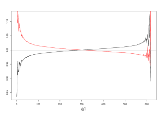
Figure 1: Plot of $\alpha_{b}(4,a_{1})$ (black) and $\alpha_{b}(v_{1}=10,a_{1})$ (red)

The variability of $N_{b}(v,a1)$ around its mean seems to be controlled. The figure 2 shows that the $54$ values of $\sum_{a_{1}=1,54}N_{b}(v,a1)$ with $v\in V,$ lie between 5174 and 6520. The values are clustered in 22 groups, 6 groups with one element and 16 with 3 elements. The values of $v_{1}$ for the 3-elements groups are separated by $54$: for example the group composed with $v_{1}=4,58,112$ is such that $\sum_{a_{1}=1,54}N_{b}(v,a1)=5604.$ The mean of $\sum_{a_{1}=1,54}N_{b}(v,a1)$ is $5856.5=\binom{54}{4}3^{-4}$ and the standard deviation is equal to $433.2$. This pattern is produced by equation (1).

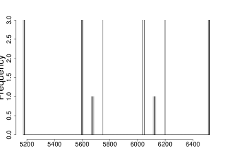
Figure 2: Histogram of $\sum_{a_{1}=1,54}N_{b}(v,a1)$ for $v\in V$

4.3 Another lower bound with $v_{1}$=4

$v_{1}=4$ is the lower possible value of $v_{1}$ and gives $n=5$ for $b=1$. $v_{2}=1$ implies that $n=3$ for $b=2$. Therefore $v_{2}\geq 3$ for all elements of $g_{5}^{*}(1)$ and $b>2$.

$$M(b,x) \geq \sum_{a_{1}\leq a(x)-4-2}N(4,a_{1})$$

$$\geq \sum_{a_{1}\leq a(x)-6}\alpha_{b}(4,a_{1})\overline{N_{b}(a_{1})}$$

$$\geq 3/m\sum_{a_{1}\leq a(x)-6}\alpha_{b}(4,a_{1})\binom{b-1}{a_{1}}_{m}$$

If Condition C1 ($a(x)<m+b-1$) is true,

$$M(b,x) \geq \frac{3}{m}\sum_{a_{1}\leq a(x)-6}\alpha_{b}(4,a_{1})\binom{a_{1}-1}{b-2}$$

$$\geq \frac{3}{m}\sum_{a_{1}=b-1}^{a(x)-6}\alpha_{b}(4,a_{1})\binom{a_{1}-1}{b-2}$$

If $\forall a_{1},\;\alpha_{b}(4,a_{1})=1$,

$$M(b,x) \geq \frac{3}{m}\sum_{a_{1}=b-1}^{a(x)-6}\binom{a_{1}-1}{b-2}$$

$$\geq \frac{3}{m}\binom{a(x)-6}{b-1}$$

$$\geq \frac{3}{2}\binom{a(x)-6}{b-1}3^{-b+1}$$

$M_{3}(x)=\sum_{b=1}^{\infty}\frac{3}{2}\binom{a(x)-6}{b-1}3^{-b+1}$ is thus another approximation of $M(x)$ and $M_{3}(x)<M_{2}(x)$.

5 Step 3: closed form for $\sum_{b=1}^{\infty}\frac{3}{2}\binom{a(x)-4}{b}3^{-b}.$

Proposition 3.

$$\sum_{b=0}^{\infty}3^{-b}\binom{b\log_{2}(3)+\log_{2}(x)}{b}=\frac{2x}{2-\log_{2}(3)}.$$

Proof.

The generalized binomial series $B_{t}(z)=\sum_{n=0}^{\infty}\binom{tn+1}{n}\frac{1}{tn+1}z^{n}$ with $n$ integer and $t,z,r$ real, has the following property, see ( [6], eq. 5.61):

$$\frac{[B_{t}(z)]^{r}}{1-t+\frac{t}{B_{t}(z)}}=\sum_{n=0}^{\infty}\binom{tn+r}{n}z^{n}$$

Another property of $B_{t}(z)$ is given in [6], eq. 5.59:

$$[B_{t}(z)]^{1-t}-[B_{t}(z)]^{-t}=z$$

that may be written $B_{t}(z)-1=z[B_{t}(z)]^{t}$
Let $z=1/3$ and $t=\log_{2}(3)$, we obtain

$B_{\log_{2}(3)}(1/3)-\frac{1}{3}[B_{\log_{2}(3)}(1/3)]^{{\log_{2}(3)}}=1.$ The equation

$$x-\frac{1}{3}x^{log_{2}3}-1=0$$

possesses only two roots: $2$ and $4$. Therefore

$$B_{\log_{2}(3)}(1/3) = \sum_{n=0}^{\infty}\binom{\log_{2}(3)n+1}{n}\frac{1}{\log_{2}(3)n+1}3^{-n}$$

$$= 2.$$

Therefore

$$\sum_{b=0}^{\infty}3^{-b}\binom{b\log_{2}(3)+\log_{2}(x)}{b} = \frac{\left[B_{\log_{2}(3)}(1/3)\right]^{\log_{2}(x)+1}}{B_{\log_{2}(3)}(1/3)(1-\log_{2}(3))+\log_{2}(3)}$$

$$= \frac{2^{\log_{2}(x)+1}}{2(1-\log_{2}(3))+\log_{2}(3)}$$

$$= \frac{1}{2-\log_{2}(3)}2^{\log_{2}(x)+1}$$

∎

Now we have closed form expressions for $M_{2}(x)$ and $M_{3}(x)$:

Proposition 4.

$$M_{2}(x) = \frac{3}{16}\frac{1}{2-\log_{2}(3)}x$$ (8)

$$M_{3}(x) = \frac{9}{64}\frac{1}{2-\log_{2}(3)}x$$ (9)

Proof.

$$M_{2}(x) = \frac{3}{2}\sum_{b=1}^{\infty}3^{-b}\binom{b\log_{2}(3)+\log_{2}(x)-4}{b}+1$$

$$= \frac{3}{2}\sum_{b=0}^{\infty}3^{-b}\binom{b\log_{2}(3)+\log_{2}(x)-4}{b}-\frac{1}{2}$$

$$= \frac{3}{2}\frac{1}{2-\log_{2}(3)}2^{\log_{2}(x)-4+1}-\frac{1}{2}$$

$$= \frac{3}{16}\frac{1}{2-\log_{2}(3)}2^{\log_{2}(x)}-\frac{1}{2}$$

$$= 0.45177x-\frac{1}{2}$$

$$M_{3}(x) = \frac{3}{2}\sum_{b=1}^{\infty}3^{-b+1}\binom{b\log_{2}(3)+\log_{2}(x)-6}{b-1}$$

$$= \frac{3}{2}\sum_{b=1}^{\infty}3^{-b+1}\binom{(b-1)\log_{2}(3)+\log_{2}(3)+\log_{2}(x)-6}{b-1}$$

$$= \frac{3}{2}\sum_{b=0}^{\infty}3^{-b}\binom{b\log_{2}(3)+\log_{2}(3)+\log_{2}(x)-6}{b}$$

$$= \frac{3}{2}\frac{1}{2-\log_{2}(3)}2^{\log_{2}(x)+\log_{2}(3)-6+1}$$

$$= \frac{9}{64}\frac{1}{2-\log_{2}(3)}2^{\log_{2}(x)}$$

$$= 0.3388x$$

∎

$M(x)$ is a lower bound for the number of odd integers included in $g(1)$. Therefore $2M(x)$ is a lower bound for the number of integers included in $g(1)$. The expression $M_{2}(x)$ contains the term $-\frac{1}{2}$ that is negligible, and we forget it in the following.

6 Toy example with $x=2.10^{10}$

Table 3: left : Number of odd integers less than $x=2.10^{10}$ obtained in $b$ steps ($b=1:300$) (black continuous line), lowerbound $M_{2}$ (red dashed line) right: y-axis: $\frac{M_{2}(b,x)}{M(b,x)}$, x-axis: $\frac{\log_{2}(x)}{b}$ ($b\in(200,500)$)

The values of $b$ for the $10^{10}$ odd numbers less than $x=2.10^{10}$ have been computed. The left figure of table 3 shows the number of odd integers less than $x$ obtained in exactly $b$ steps, compared with $M_{2}(b,x)$. We have $M_{2}(b,x)<M(b,x)$ for $b<150$, but this is not true for $b>200$ (see the right figure of the same table), because the approximation $M_{2}(b,x)$ is not a lower bound for the extremal lower tail of the distribution of $a$.

However the overestimation of $M_{2}(b,x)$ for large $b$ is largely compensed by the underestimation of $M_{2}(b,x)$ for $b<150$. The figure 3 shows that $\forall b\in\mathbb{N},\sum_{i=1}^{b}M_{2}(i,x)<\sum_{i=1}^{b}N(i,x)$.

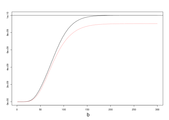
Figure 3: Number of odd integers less than $x=10^{10}$ obtained in less than $b$ steps (black continuous line) lowerbound $M_{2}$ (red dashed line)

7 Properties of the distribution $P(B=b)=\frac{8(2-\log_{2}(3))}{x}\binom{a(x)-4}{b}3^{-b}$ for fixed $x$.

For fixed $x$ let $B$ be an integer random variable defined by $P(B=b)=\frac{8(2-\log_{2}(3))}{x}\binom{a(x)-4}{b}3^{-b}$, the proportion $\frac{M_{2}(b,x)}{\sum_{b}M_{2}(b,x)}.$ There is no random process in the context of the Collatz problem. The probabilistic formalization is only a practical way to express the distribution of the values of $b$ for odd integers less than $x$. For instance, $\mathbb{E}(B)$ is an approximation of the mean value of $b$ among the odd integers less than $x$. The moments of $B$ can be expressed using the properties of the generalized binomial series $B_{t}(z)=\sum_{n=0}^{\infty}\binom{tn+1}{n}\frac{1}{tn+1}z^{n}$:

Proposition 5.

$$\mathbb{E}_{x}(B)=\frac{log_{2}(x)}{2-log_{2}(3)}+\frac{5log_{2}(3)-8}{(2-log_{2}(3))^{2}}\simeq 2.409421\log_{2}(x)-0.436487$$

Proof.

$$z\frac{\partial{\left\{\frac{B_{t}(z)^{r}}{1-t+\frac{t}{B_{t}(z)}}\right\}}}{\partial z}=\sum_{n=0}^{\infty}\binom{tn+r}{n}nz^{n},$$

and

$$z\frac{\partial{\left\{\frac{B_{t}(z)^{r+1}}{(1-t)B_{t}(z)+t}\right\}}}{\partial{z}}=z\left\{\frac{(r+1)B_{t}(z)^{{}^{\prime}}B_{t}(z)^{r}}{(1-t)B_{t}(z)+t}-\frac{(1-t)B_{t}(z)^{{}^{\prime}}B_{t}(z)^{r+1}}{((1-t)B_{t}(z)+t)^{2}}\right\}$$

Moreover

$$B_{t}(z)-1=zB_{t}(z)^{t}\Rightarrow B_{t}(z)^{{}^{\prime}}=\frac{B_{t}(z)^{t}}{1-ztB_{t}(z)^{t-1}}.$$

$z=1/3$ and $t=\log_{2}(3)\Rightarrow B_{t}(z)^{{}^{\prime}}=\frac{6}{2-\log_{2}(3)}.$

Therefore

$$\sum_{n=0}^{\infty}\binom{\log_{2}(3)n+r}{n}n\left(\frac{1}{3}\right)^{n}=\frac{2^{r+1}}{2-log_{2}(3)}\left(\frac{r+1}{2-log_{2}(3)}+\frac{2(log_{2}(3)-1)}{(2-log_{2}(3))^{2}}\right),$$

$r=\log_{2}(x)-4\Rightarrow\mathbb{E}_{x}(B)=\frac{\log_{2}(x)}{2-log_{2}(3)}+\frac{5log_{2}(3)-8}{(2-log_{2}(3))^{2}}$

∎

Proposition 6.

$$\mathbb{V}_{x}(B)=\log_{2}(x)\frac{2}{(2-log_{2}(3))^{3}}+\frac{2\log_{2}(3)^{2}+8\log_{2}(3)-16}{(2-log_{2}(3))^{4}}\simeq 27.9749\log_{2}(x)+57.4246$$

Proof.

see annex ∎

Higher moments can be computed by the same method. Moreover the pdf of $B$ tends to normality when $x$ tends to $\infty$.

Proposition 7.

$$\lim_{x\rightarrow\infty}\mathcal{L}\left(\frac{B-\mathbb{E}_{x}(B)}{\mathbb{V}_{x}(B)^{\frac{1}{2}}}\right)=\mathcal{N}(0,1)$$

Proof.

see annex ∎

The proposition 7 may be used to cut the last terms of $M_{2}(x).$ Actually the proposed minoration $M_{2}(b,x)$ of $M(b,x)$ prove defective for high values of $b$ such that $\frac{\log_{2}(x)}{b}<0.25\Leftrightarrow b>4\log_{2}(x)$. For large $x$:

$$M^{\prime}_{2}(x)=\frac{3}{2}\sum_{b=\mathbb{E}_{x}(B)-2\sqrt{\mathbb{V}_{x}(B)}}^{\mathbb{E}_{x}(B)+2\sqrt{\mathbb{V}_{x}(B)}}3^{-b}\binom{b\log_{2}(3)+\log_{2}(x)-4}{b}\simeq 0.954M_{2}(x)=\frac{3}{16}\frac{0.954}{2-\log_{2}(3)}x.$$

Moreover for large $x$,

$$\mathbb{E}_{x}\left(\frac{B}{\log_{2}(x)}\right)+2\sqrt{\mathbb{V}_{x}\left(\frac{B}{\log_{2}(x)}\right)} = 2.41-\frac{0.44}{\log_{2}(x)}+2\sqrt{\frac{27.9749}{\log_{2}(x)}+\frac{57.4246}{(\log_{2}(x))^{2}}}$$

$$< 4$$

The concentration of the pdf of $\frac{B}{\log_{2}(x)}$ around $\mathbb{E}_{x}\left(\frac{B}{\log_{2}(x)}\right)$ implies that the problem of the defective large values of $b$ in $M_{2}(x)$ vanishes when $x\rightarrow\infty$. The same argument applies to the low values of $b<\log(\log_{2}(x))+1$ for which the condition C1 is not valid.

Appendix A Proof of proposition 6.

$$z^{2}\frac{\partial^{2}{\left\{\frac{B_{t}(z)^{r}}{1-t+\frac{t}{B_{t}(z)}}\right\}}}{\partial^{2}z}=\sum_{n=0}^{\infty}\binom{tn+r}{n}n(n-1)z^{n},$$

and

$$\frac{\partial^{2}{\frac{B_{t}(z)^{r+1}}{(1-t)B_{t}(z)+t}}}{\partial^{2}{z}}=\frac{\partial{\left\{\frac{(r+1)B_{t}(z)^{{}^{\prime}}B_{t}(z)^{r}}{(1-t)B_{t}(z)+t}-\frac{(1-t)B_{t}(z)^{{}^{\prime}}B_{t}(z)^{r+1}}{((1-t)B_{t}(z)+t)^{2}}\right\}}}{\partial z}$$

$$\frac{\partial{\frac{(r+1)B_{t}(z)^{{}^{\prime}}B_{t}(z)^{r}}{(1-t)B_{t}(z)+t}}}{\partial z} = (r+1)\left[\frac{rB_{t}(z)^{{}^{\prime}2}B_{t}(z)^{r-1}+B_{t}(z)^{{}^{\prime\prime}}B_{t}(z)^{r}}{(1-t)B_{t}(z)+t}-\frac{B_{t}(z)^{{}^{\prime}2}B_{t}(z)^{r}(1-t)}{((1-t)B_{t}(z)+t)^{2}}\right]$$

$$\frac{\partial{\frac{(1-t)B_{t}(z)^{{}^{\prime}}B_{t}(z)^{r+1}}{((1-t)B_{t}(z)+t)^{2}}}}{\partial z} = (1-t)\left[\frac{B_{t}(z)^{{}^{\prime\prime}}B_{t}(z)^{r+1}+(r+1)B_{t}(z)^{{}^{\prime}2}B_{t}(z)^{r}}{((1-t)B_{t}(z)+t)^{2}}\right]$$

$$- 2(1-t)\frac{(1-t)B_{t}(z)^{{}^{\prime}2}B_{t}(z)^{r+1}}{((1-t)B_{t}(z)+t)^{3}}$$

Moreover, with $c=(2-t),$

$$B_{t}(z)^{\prime\prime} = \left(\frac{B_{t}(z)^{t}}{1-ztB_{t}(z)^{t-1}}\right)^{\prime}$$

$$= \frac{tB_{t}(z)^{t-1}B_{t}(z)^{\prime}}{1-ztB_{t}(z)^{t-1}}+B_{t}(z)^{t}\frac{tB_{t}(z)^{t-1}+zt(t-1)B_{t}(z)^{t-2}B_{t}(z)^{\prime}}{((1-ztB_{t}(z)^{t-1})^{2}}$$

$$= \frac{t2^{t-1}6/c}{1-(1/3)t2^{t-1}}+2^{t}\frac{t2^{t-1}+(1/3)t(t-1)2^{t-2}6/c}{((1-(1/3)t2^{t-1})^{2}}$$

$$= \frac{t\frac{3}{2}6/c}{1-(1/3)t\frac{3}{2}}+3\frac{t\frac{3}{2}+(1/3)t(t-1)\frac{3}{4}6/c}{((1-(1/3)t\frac{3}{2})^{2}}$$

$$= \frac{18t}{c^{2}}+3\frac{6tc+6t(t-1)}{c^{3}}$$

$$= \frac{18t}{c^{2}}\left(1+\frac{c+(t-1)}{c}\right)$$

$$= \frac{18t}{c^{3}}\left(2c+(t-1)\right)$$

$$= \frac{18t}{c^{3}}(3-t)$$

$$= \frac{18\log_{2}(3)(3-\log_{2}(3))}{(2-\log_{2}(3))^{3}}$$

With $t=\log_{2}3,z=\frac{1}{3}\Rightarrow B_{t}(z)=2,B_{t}(z)^{\prime}=\frac{6}{c}$ and $B_{t}(z)^{\prime\prime}=d$ we obtain

$$\frac{\partial{\frac{(r+1)B_{t}(z)^{{}^{\prime}}B_{t}(z)^{r}}{(1-t)B_{t}(z)+t}}}{\partial z} = (r+1)\left[\frac{r(\frac{6}{c})^{2}2^{r-1}+d2^{r}}{c}-\frac{(\frac{6}{c})^{2}2^{r}(1-t)}{c^{2}}\right]$$

$$= \frac{(r+1)2^{r}}{c^{4}}\left(18rc+dc^{3}-36(1-t)c\right)$$

$$= \frac{(r+1)2^{r}}{c^{4}}\left(18rc+18t(3-t)-36(1-t)\right)$$

$$= \frac{18(r+1)2^{r}}{c^{4}}\left(r(2-t)+t(3-t)-2(1-t)\right)$$

$$= \frac{18(r+1)2^{r}}{c^{4}}\left(rc+5t-t^{2}-2\right)$$

$$= 9\frac{2^{r+1}}{c^{5}}\left((r+1)(rc^{2}+(5t-t^{2}-2)c)\right)$$

and

$$\frac{\partial{\frac{(1-t)B_{t}(z)^{{}^{\prime}}B_{t}(z)^{r+1}}{((1-t)B_{t}(z)+t)^{2}}}}{\partial z} = (1-t)\left[\frac{d2^{r+1}+(r+1)(1-t)(\frac{6}{c})^{2}2^{r}}{((1-t)2+t)^{2}}-2\frac{(1-t)(\frac{6}{c})^{2}2^{r+1}}{((1-t)2+t)^{3}}\right]$$

$$= \frac{(1-t)2^{r+1}}{c^{5}}\left(dc^{3}+18(r+1)c-72(1-t)\right)$$

$$= \frac{(1-t)2^{r+1}}{c^{5}}\left((18t(3-t)+18(r+1)c-72(1-t)\right)$$

$$= 18\frac{(1-t)2^{r+1}}{c^{5}}\left(t(3-t)+(r+1)c-4(1-t)\right)$$

$$= 18\frac{(1-t)2^{r+1}}{c^{5}}\left((r+1)c-t^{2}+7t-4\right)$$

$$= 9\frac{2^{r+1}}{c^{5}}\left(2(1-t)((r+1)c-t^{2}+7t-4)\right)$$

and

$$z^{2}\frac{\partial^{2}{\left\{\frac{B_{t}(z)^{r}}{1-t+\frac{t}{B_{t}(z)}}\right\}}}{\partial^{2}z} = \frac{2^{r+1}}{c^{5}}\left((r+1)(rc^{2}+(5t-t^{2}-2)c)-2(1-t)((r+1)c-t^{2}+7t-4)\right)$$

$$= \frac{2^{r+1}}{c^{5}}\left(r(r+1)c^{2}+c(r+1)(5t-t^{2}-2-2(1-t))-2(1-t)(-t^{2}+7t-4)\right)$$

$$= \frac{2^{r+1}}{c^{5}}\left(r(r+1)c^{2}+c(r+1)(-t^{2}+7t-4)+2(t-1)(-t^{2}+7t-4)\right)$$

Therefore

$$\sum_{n=0}^{\infty}\binom{\log_{2}(3)n+r}{n}n(n-1)\left(\frac{1}{3}\right)^{n}=\frac{2^{r+1}}{c^{5}}\left(r(r+1)c^{2}+(r+1)c(-t^{2}+7t-4)+2(t-1)(-t^{2}+7t-4)\right),$$

$r=\log_{2}(x)-4\Rightarrow\mathbb{E}(B(B-1))=\frac{1}{c^{4}}\left((l-4)(l-3))c^{2}+(l-3)c(-t^{2}+7t-4)+2(t-1)(-t^{2}+7t-4)\right)$ and with $l=\log_{2}x$,

$$\mathbb{V}(B) = \mathbb{E}(B(B-1)+\mathbb{E}(B)-\mathbb{E}(B)^{2}$$

$$= \frac{1}{c^{4}}\left((l-4)(l-3)c^{2}+(l-3)c(-t^{2}+7t-4)+2(t-1)(-t^{2}+7t-4)\right)$$

$$+ \frac{l}{c}+\frac{5t-8}{c^{2}}-(\frac{l}{c}+\frac{5t-8}{c^{2}})^{2}$$

$$= \frac{l(4-2t)+2t^{2}+8t-16}{c^{4}}$$

Appendix B Proof of proposition 7.

Let $g_{B_{x}}(s)$ the generating function of $B.$ With $t=\log_{2}3,$ $l=\log_{2}x-4$ and $c=2-t$,

$$g_{B_{x}}(s) = \sum_{b=0}^{\infty}s^{b}P_{x}(B=b)$$

$$= \sum_{b=0}^{\infty}s^{b}\frac{8(2-\log_{2}(3))}{x}\binom{a(x)-4}{b}3^{-b}$$

$$= \frac{8(2-t)}{x}\sum_{b=0}^{\infty}\left(\frac{s}{3}\right)^{b}\binom{bt+\log_{2}x-4}{b}$$

$$= \frac{2-t}{2}2^{4-\log 2x}\sum_{b=0}^{\infty}\left(\frac{s}{3}\right)^{b}\binom{bt+\log_{2}x-4}{b}$$

$$= \frac{c}{2}2^{-l}\sum_{b=0}^{\infty}\left(\frac{s}{3}\right)^{b}\binom{bt+l}{b}$$

$$= c2^{-(l+1)}\frac{[B_{t}(\frac{z}{3})]^{l+1}}{(1-t)B_{t}(\frac{z}{3})+t}$$

$x\rightarrow\infty\Rightarrow\frac{\mathbb{E}(B)}{\mathbb{V}(B)^{\frac{1}{2}}}=\sqrt{\frac{lc}{2}}+o(l^{\frac{1}{2}}),$ and $\frac{1}{\mathbb{V}(B)^{\frac{1}{2}}}=c\sqrt{\frac{c}{2l}}+o(l^{-\frac{1}{2}}).$

Therefore the generating function of $\frac{B-\mathbb{E}(B)}{\mathbb{V}(B)^{\frac{1}{2}}}$ is $h_{x}(s)=s^{-\sqrt{\frac{lc}{2}}}g_{B_{x}}(s^{c\sqrt{\frac{c}{2l}}}).$

$$h_{x}(s) = s^{-\sqrt{\frac{lc}{2}}}\frac{c}{2}2^{-l}\frac{[B_{t}(\frac{s^{c\sqrt{\frac{c}{2l}}}}{3})]^{l+1}}{(1-t)B_{t}(\frac{s^{c\sqrt{\frac{c}{2l}}}}{3})+t}$$

Let $\phi_{x}(u)=h_{x}(e^{u})$ with $y=l^{-1},$ one obtains

$$\phi_{x}(u) = e^{-u\sqrt{\frac{lc}{2}}}c2^{-l-1}\frac{[B_{t}(\frac{e^{uc\sqrt{\frac{c}{2l}}}}{3})]^{l+1}}{(1-t)B_{t}(\frac{e^{uc\sqrt{\frac{c}{2l}}}}{3})+t}$$

$$\log(\phi_{x}(u)) = -u\sqrt{\frac{lc}{2}}+(l+1)\left[\log[B_{t}(\frac{e^{uc\sqrt{\frac{c}{2l}}}}{3})-\log 2\right]-\left[\log((1-t)B_{t}(\frac{e^{uc\sqrt{\frac{c}{2l}}}}{3})+t)-\log(c)\right]$$

$$\log(\phi_{x}(u)) = -u\sqrt{\frac{c}{2y}}+(\frac{1}{y}+1)\left[\log[B_{t}(\frac{e^{uc\sqrt{\frac{cy}{2}}}}{3})-\log 2\right]-\left[\log((1-t)B_{t}(\frac{e^{uc\sqrt{\frac{cy}{2}}}}{3})+t)-\log(c)\right]$$

Let $A=u\sqrt{\frac{c^{3}}{2}},$ $e^{A\sqrt{y}}=1+A\sqrt{y}+\frac{1}{2}A^{2}y+o(y)$,

and $B_{t}(z/3)=B_{t}(1/3)+(z-1)B^{\prime}_{t}(1/3)+\frac{1}{2}(z-1)^{2}B^{\prime\prime}_{t}(1/3)+o(z^{2})$ the Taylor expansion of $B_{t}(z)$ in the neighborhood of one.

$$B_{t}\left(\frac{e^{A\sqrt{y}}}{3}\right) = B_{t}(\frac{1}{3})+A\sqrt{y}+\frac{1}{2}A^{2}yB^{\prime}_{t}(1/3)+\frac{1}{2}\left(A\sqrt{y}+\frac{1}{2}A^{2}y\right)^{2}B^{\prime\prime}_{t}(1/3)+o(y)$$

$$= 2+2\frac{A}{c}\sqrt{y}+\frac{A^{2}}{c^{3}}y(4-t)+o(y)$$

$$\frac{B_{t}\left(\frac{e^{A\sqrt{y}}}{3}\right)}{B_{t}(\frac{1}{3})} = 1+\frac{A}{c}\sqrt{y}+\frac{A^{2}}{2c^{3}}y(4-t)+o(y)$$

$$\log\left[\frac{B_{t}\left(\frac{e^{A\sqrt{y}}}{3}\right)}{B_{t}(\frac{1}{3})}\right] = \frac{A}{c}\sqrt{y}+\frac{A^{2}}{2c^{3}}y(4-t)-\frac{1}{2}\left(\frac{A}{c}\sqrt{y}\right)^{2}+o(y)$$

$$= \frac{A}{c}\sqrt{y}+\frac{A^{2}}{c^{3}}y+o(y)$$

$$(1+\frac{1}{y})\log\left[\frac{B_{t}\left(\frac{e^{A\sqrt{y}}}{3}\right)}{B_{t}(\frac{1}{3})}\right] = \frac{A}{c}y^{-\frac{1}{2}}+\frac{A^{2}}{c^{3}}+o(1)$$

$$= u\sqrt{\frac{c}{2}}y^{-\frac{1}{2}}+\frac{u^{2}}{2}+o(1)$$

$$\log(\phi_{x}(u)) = -u\sqrt{\frac{c}{2y}}+u\sqrt{\frac{c}{2}}y^{-\frac{1}{2}}+\frac{u^{2}}{2}+o(1)$$

$$= \frac{u^{2}}{2}+o(1)$$

Note that $\log((1-t)B_{t}(\frac{e^{uc\sqrt{\frac{cy}{2}}}}{3})+t)-\log(c)=O(y^{\frac{1}{2}})$ and does not contribute to the limit of $\log(\phi_{x}(u)).$

Therefore $\lim_{x\rightarrow\infty}\phi_{x}(u)=e^{\frac{u^{2}}{2}}$ , the gaussian moment generating function.

References

- [1] David Applegate and Jeffrey C. Lagarias. Density bounds for the problem. Math. Comp., (64):427–438, 1995.
- [2] Livio Colussi. The convergence classes of Collatz function. Theoretical Computer Science, 412(39):5409–5419, 2011.
- [3] J-J. Daudin and L. Pierre. A simple proof of the Wirsching-Goodwin representation of integers connected to 1 in the 3x+1 problem. arXiv:1507.07968v2 [math.NT], 2016.
- [4] Steffen Eger. Restricted Weighted Integer Compositions and Extended Binomial Coefficients. Journal of Integer Sequences, 16, 2013.
- [5] J. R. Goodwin. The 3x+1 Problem and Integer Representations. arXiv:1504.03040 [math.NT], 2015.
- [6] R. L. Graham, D. E. Knuth, and O. Patashnik. Concrete mathematics. Addison-Wesley Publishing Company, 1994.
- [7] I. Krasikov. How many numbers satisfy the 3x+1 conjecture ? Internat. J. Math. Math. Sci., 12:791–796, 1989.
- [8] Ilia Krasikov and Jeffrey C. Lagarias. Bounds for the 3x+1 Problem using Difference Inequalities. arXiv:math/0205002v1 [math.NT], 2002.
- [9] J.C. Lagarias. The Ultimate Challenge: The 3x+1 Problem. American Mathematical Soc., 2010.
- [10] T. Neuschel. A Note on Extended Binomial Coefficients. arXiv:1407.7429 [math.CO], 2014.