Vortex solitons in fractional nonlinear Schrödinger equation with the cubic-quintic nonlinearity

Abstract

We address the existence and stability of vortex-soliton (VS) solutions of the fractional nonlinear Schrödinger equation (NLSE) with competing cubic-quintic nonlinearities and the Lévy index (fractionality) taking values $1\leq\alpha\leq 2$. Families of ring-shaped VSs with vorticities $s=1,2$, and $3$ are constructed in a numerical form. Unlike the usual two-dimensional NLSE (which corresponds to $\alpha=2$), in the fractional model VSs exist above a finite threshold value of the total power, $P$. Stability of the VS solutions is investigated for small perturbations governed by the linearized equation, and corroborated by direct simulations. Unstable VSs are broken up by azimuthal perturbations into several fragments, whose number is determined by the fastest growing eigenmode of small perturbations. The stability region, defined in terms of $P$, expands with the increase of $\alpha$ from $1$ up to $2$ for all $s=1$, $2$, and $3$, except for steep shrinkage for $s=2$ in the interval of $1\leq\alpha\leq 1.3$.

I Introduction

It is well known that optical beams propagating in conservative and dissipative self-focusing media readily build spatial optical solitons, which are a subject of great interest to fundamental and applied studies in diverse settings Trillo -Rosanov2 . In particular, a class of 2D vortex solitons (VSs) feature a bright ring shape with an embedded rotating screw phase dislocation, see early original works early -early6 and early reviews Review1 -RaduVolkov , as well as recent ones Review2 -Review6 . VSs usually represent excited states of the corresponding nonlinear systems. In particular, VSs in the simplest two-dimensional (2D) model, based on the nonlinear Schrödinger equation (NLSE) with cubic self-focusing Kruglov-PLA1985 , may be considered as excited states of the fundamental mode known as Townes solitons TownesSoliton . In models with basic self-attractive nonlinearities, such as those represented by quadratic and cubic terms, self-trapped vortex states are subject to azimuthal symmetry-breaking instabilities which split them into sets of fragments, that may be fundamental solitons Ele-Lett33-608 ; PRL79-2450 . Therefore, stability is a crucially important issue in studies of VSs. Several methods for the stabilization of VSs in nonlinear media without the help of external potentials were suggested, such as the use of competing quadratic-cubic QC1 -QC3 and cubic-quintic (CQ) CQ1 -CQ12 nonlinearities, or, alternatively, nonlocal self-interaction Nonlocal1 -Nonlocal7 . In this connection, it is relevant to mention that exact solutions for stable 1D solitons of the NLSE with the CQ nonlinearity were first obtained in early work Bulgaria .

Recently, the Schrödinger equation was extended to fractional dimensions, starting from works by Y. Hu and N. Laskin in Ref. FSE1a ; FSE1b . The fractional Schrödinger equation (FSE) was introduced as a quantum model FSE2 , in which Feynman path integrals over Brownian trajectories lead to the standard Schrödinger equation, while path integrals over “skipping” Lévy trajectories lead to the FSE FSE3 . Although implications of such theories are still a matter of debate FSE4 ; FSE5 , experimental schemes have been proposed for their realization in condensed-matter settings and optics FSE11 ; FSE12 . In particular, optical cavities offer an appropriate ground to explore intriguing properties of the FSE. Propagation of beams has been intensively studied in the framework of FSE, producing effects such as zigzag trajectories FSE13 , diffraction-free propagation FSE14 -FSE18 , beam splitting FSE19 , periodically oscillating evolution of Gaussian modes FSE20 , beam-propagation management FSE21 , optical Bloch oscillations and Zener tunneling FSE22 , resonant mode conversions and Rabi oscillations FSE23 , Anderson localization and delocalization FSE24 , and $\mathcal{PT}$-symmetric optical modes FSE25 .

A natural extension of the analysis is to add nonlinearity to the FSE NLFSE2 ; NLFSE3 . In particular, the 1D Schrödinger equation with the cubic term subject to singular spatial modulation may emulate fractional dimension $0<D<1$ Olga . Recent works have demonstrated that the fractional NLSE supports a variety of fractional spatial-soliton solutions NLFSE4 : “accessible solitons” NLFSE5 -NLFSE7 , double-hump and fundamental solitons in $\mathcal{PT}$-symmetric potentials NLFSE8 ; NLFSE9 , bulk and surface gap solitons in $\mathcal{PT}$-symmetric photonic lattices NLFSE10 -NLFSE11a , vortex solitons in $\mathcal{PT}$-symmetric azimuthal potentials NLFSE11b , 2D self-trapped modes NLFSE12a , spontaneous symmetry breaking in a dual-core system we , and dissipative solitons in the fractional complex-Ginzburg-Landau equation Yingji . Further, the composition relation between nonlinear Bloch waves and gap solitons supported by lattices NLFSE14 ; NLFSE12b , solitons under the action of nonlinearity subject to spatially-periodic modulation NLFSE15 , dissipative surface solitonsNLFSE15b , as well as discrete solitons NLFSE15d , have also been addressed. Recently, off-site- and on-site-centered VSs in $\mathcal{PT}$-symmetric photonic lattices have been investigated in Ref. NLFSE13 . However, prediction of spatial VS solutions in free space (without the use of external potentials) in the framework of fractional NLSE is still an open problem. This issue is addressed in the present work.

The paper is organized as follows. The model is introduced in Sec. II, which is followed by the analysis of the stability and dynamics of vortex-soliton states in Sec. III. The paper is concluded by Sec. IV.

II The model

We start the analysis by considering the beam propagation along the $z$-axis in a nonlinear isotropic medium with the CQ nonlinear correction to refractive index, $n_{\mathrm{nonlin}}(I)=n_{2}I-n_{4}I^{2}$, where $I$ is the light intensity, while $n_{2}$ and $n_{4}$ are coefficients accounting for, respectively, cubic self-focusing and quintic defocusing. The respective fractional NLSE is

$$2ik_{0}\frac{\partial A}{\partial z}-\left(-\nabla_{\perp}^{2}\right)^{\alpha/2}A+\frac{2k_{0}^{2}}{n_{0}}n_{\mathrm{nonlin}}A=0,$$ (1)

where $A(z,x)$ is the local amplitude of the optical field, the intensity being $I\equiv|A|^{2}$, $k_{0}=2\pi n_{0}/\lambda$ is the wavenumber, with background refractive index $n_{0}$ and optical wavelength $\lambda$, while $-(-\nabla_{\perp}^{2})^{\alpha/2}=-(-\partial^{2}/\partial x^{2}-\partial^{2}/\partial y^{2})^{\alpha/2}$ is the fractional-diffraction operator with the corresponding Lévy index $\alpha$ belonging to interval $1<\alpha\leq 2$. Equation (1) with $\alpha\leq 1$ and cubic-only self-focusing gives rise to the wave collapse, which destabilizes solitons; however, the quintic self-defocusing term suppresses the instability and, in particular, makes it possible to construct stable VSs at $\alpha=1$, as shown below.

The balance between the fractional diffraction and nonlinearity makes it possible to build spatial solitons. By means of rescaling, $\Psi(\zeta,\xi)=\sqrt{n_{4}/n_{2}}A(z,x)$, $\zeta=\left(k_{0}n_{2}^{2}/n_{0}n_{4}\right)z$, and $\left(\xi,\eta\right)=\left(2k_{0}^{2}n_{2}^{2}/n_{0}n_{4}\right)^{1/\alpha}\left(x,y\right)$, Eq. (1) is cast in the normalized CQ form,

$$i\frac{\partial\Psi}{\partial\zeta}-\left(-\nabla_{\perp}^{2}\right)^{\alpha/2}\Psi+\left|\Psi\right|^{2}\Psi-\left|\Psi\right|^{4}\Psi=0.$$ (2)

Obviously, when $\alpha=2$ Eq. (2) reduces to the conventional cubic-quintic NLSE CQ12 .

In this paper, we aim to construct spatial vortex-soliton solutions to Eq. (2), with propagation constant $\beta$, as

$$\Psi\left(\zeta,\xi,\eta\right)=\psi\left(\xi,\eta\right)e^{i\beta\zeta},$$ (3)

where complex function $\psi(\xi,\eta)$ obeys a stationary equation:

$$-\left(-\nabla_{\perp}^{2}\right)^{\alpha/2}\psi+\left|\psi\right|^{2}\psi-\left|\psi\right|^{4}\psi-\beta\psi=0.$$ (4)

Further, the complex function is expressed in the Madelung’s form, $\psi(\xi,\eta)=U(\xi,\eta)e^{i\phi(\xi,\eta)}$, where real functions $U(\xi,\eta)$ and $\phi(\xi,\eta)$ represent the amplitude and phase of the solution. In polar coordinates $(r,\theta)$, related to the underlying Cartesian coordinates by the usual formulas, $\xi=r\cos\theta$, $\eta=r\sin\theta$, VSs are expressed as

$$\psi(r,\theta)=U(r)e^{is\theta},$$ (5)

where positive integer $s$ represents the vorticity (topological charge of the phase screw dislocation), and the optical intensity vanishes as $\left|A\right|^{2}\sim r^{2s}$ at $r\rightarrow 0$. The power (integral norm) and total angular momentum of the vortex are

$$P=\int\int\left|\psi\left(\xi,\eta\right)\right|^{2}d\xi d\eta,$$ (6)

$$L=\int\int\frac{\partial\phi(\xi,\eta)}{\partial\theta}\left|\psi\left(\xi,\eta\right)\right|^{2}d\xi d\eta.$$ (7)

As it follows from Eqs. (5)-(7), for stationary VSs the angular momentum and power are related by $L=sP$.

III Numerical results

III.1 The numerical method

The fractional Laplacian in the FSE is defined as a pseudo-differential operator JMP51-062102 ; JMP54-012111 ; CMA71 ,

$$\mathcal{F}[\left(-\nabla_{\perp}^{2}\right)^{\alpha/2}\psi\left(\xi,\eta\right)]=\left(k_{\xi}^{2}+k_{\eta}^{2}\right)^{\alpha/2}\hat{\psi}(k_{\xi},k_{\eta}),$$ (8)

where $\mathcal{F}$ is the operator of the Fourier transform, and $\hat{\psi}(k_{\xi},k_{\eta})$ is the Fourier image of $\psi(\xi,\eta)$. Below, we construct vortex-soliton solutions of Eq. (4) with fractional values of Lévy index $\alpha$ by means of the Newton-conjugate-gradient method NCG ; Book1 . For the sake of comparison, we will also present usual solutions for $\alpha=2$. Following this method, Eq. (4) is rewritten in the form of

$$\Lambda_{0}\psi\left(\xi\right)=0,$$ (9)

where the operator is defined as

$$\Lambda_{0}=-\left(-\nabla_{\perp}^{2}\right)^{\alpha/2}+\left|\psi\right|^{2}-\left|\psi\right|^{4}-\beta.$$ (10)

Here, the propagation constant $\beta$ is considered as a given value, and the solution is calculated by means of Newton iterations,

$$\psi_{n+1}=\psi_{n}+\Delta\psi_{n},$$ (11)

where $\psi_{n}$ is an approximate solution, and $\Delta\psi_{n}$ is computed from the linear Newton-correction equation,

$$L_{1n}\Delta\psi_{n}=-L_{0}\left(\psi_{n}\right),$$ (12)

with $L_{1n}$ being the linearization operator of Eq. (9), evaluated with the approximate solution $\psi_{n}$:

$$L_{1} = \left.-\left(-\nabla_{\perp}^{2}\right)^{\alpha/2}+\left|\psi\right|^{2}-\left|\psi\right|^{4}-\beta+\right.$$ (14)

$$\left.2\psi\mathtt{Re}\left(\psi^{\ast}\right)-4\left|\psi\right|^{2}\psi\mathtt{Re}\left(\psi^{\ast}\right).\right.$$

Then, Eq. (12) can be solved directly by dint of preconditioned conjugate gradient iterations NCG ; Book1 .

III.2 Vortex-soliton (VS) solutions

To quantify numerically found families of VS solutions with different vorticities $s$ and different values of the Lévy index $\alpha$, we display respective dependencies of their propagation constant $\beta$ on power $P$ in Fig. 1 (stability and instability of the families represented by the solid blue and dotted red lines, respectively, is identified below by the linear-stability analysis and direct simulations). It is seen that the celebrated Vakhitov-Kolokolov criterion ($d\beta/dP>0$) VK ; Fibich is only a necessary but not sufficient condition for the stability of the VS solutions belonging to the upper branches in Figs. 1(a-d). The limit value of the power for stable (upper) branches of the $\beta(P)$ dependencies is $\beta_{\max}=3/16$, which is a known feature of the CQ nonlinearity, that does not depend on the dimension CQ1 -CQ12 . In the limit of $\beta=\beta_{\max}$, the soliton (in any dimension) carries over into an exact 1D front solution (alias domain wall), which connects zero intensity, $\left|\psi\right|^{2}=0$, and the largest value achievable in the soliton, $\left(\left|\psi\right|^{2}\right)_{\max}\equiv\left|\psi\left(\beta=3/16\right)\right|^{2}=3/4$ Birnbaum :

$$\Psi\left(\xi,\zeta\right)=\exp\left(\frac{3}{16}i\zeta\right)\sqrt{\frac{3/4}{1+\exp\left(\pm\sqrt{3}\xi/2\right)}}.$$ (15)

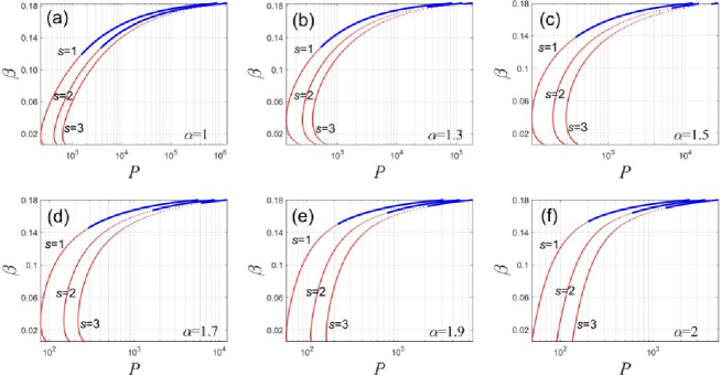
Figure 1: (Color online) The propagation constant of vortex solitons versus their integral power, for vorticities $s=1,2,3$, and different values of the Lévy index: (a) $\alpha=1$, (b) $\alpha=1.3$, (c) $\alpha=1.5$, (d) $\alpha=1.7$, (e) $\alpha=1.9$, and (f) $\alpha=2$. The latter case, corresponding to the usual NLSE, is included for comparison with the results produced by the fractional equation. Here, solid blue and dotted red curves denote stable and unstable solutions, respectively. The limit value of the upper branches at $P\rightarrow\infty$ is $\beta_{\max}=3/16$, see the text.

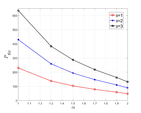
Figure 2: (Color online) Dependence of $P_{\mathrm{thr}}$ on the Lévy index $\alpha$ of the vortex-soliton solutions for vorticities $s=1,2,3$.

The comparison of panels (a-e) and (f) in Fig. 1 demonstrates that, at all values of the Lévy index $\alpha<2$, there is a threshold (minimum) value of the total power, $P_{\mathrm{thr}}$, necessary for the existence of the VS solutions and, accordingly, there are two branches of the $\beta(P)$ curves, which merge at $P=P_{\mathrm{thr}}$. In fact, this feature is similar to one demonstrated by the CQ model in the 3D case CQ2a ; CQ2b ; CQ8 ; CQ9 , and the nonexistence of solitons at $P<P_{\mathrm{thr}}$ is explained by the fact the weak nonlinearity cannot balance the fractional-order diffraction. On the contrary, the threshold vanishes in the limit of $\alpha=2$, which corresponds to the usual CQ model in 2D. Dependence of the threshold value of the total power $P_{\mathrm{thr}}$ on the Lévy index $\alpha$ is displayed in Fig. 2.

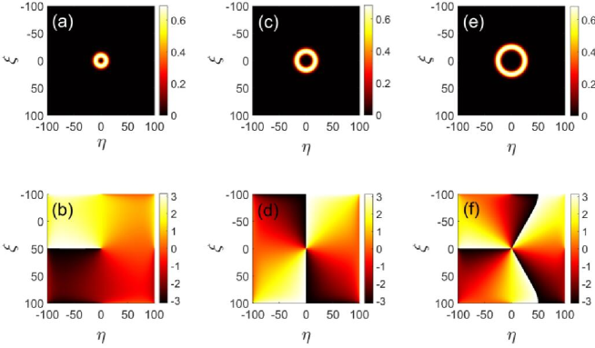
Figure 3: (Color online) Intensity and phase patterns of the vortex-soliton solutions with propagation constant $\beta=0.14$, Lévy index $\alpha=1.5$, and vorticities (a,b) $s=1$ (the 2D soliton is stable), (c,d) $s=2$ (unstable), (e,f) $s=3$ (unstable).

Typical examples of intensity and phase profiles of the numerically generated VS solutions, with $s=1$, $2$ and $3$, are displayed in Fig. 3 for $\alpha=1.5$. Further, cross-section profiles of the VS modes, in the form of $\left|\psi\left(\xi,\eta=0\right)\right|$, are displayed in Fig. 4, for propagation constants $\beta$ ranging from $0.006$ to $0.18$, which demonstrates the well-known property of systems with competing nonlinearities, viz., a trend to the formation of flat-top shapes of the solitons in the limit of large powers (i.e., $\beta\rightarrow\beta_{\max}=3/16$, $|\psi|^{2}\rightarrow 3/4$). Further, Fig. 4 demonstrates that the solitons’ profiles additionally expand with the decrease of the Lévy index, $\alpha$. This trend is explained by the fact that decrease of $\alpha$ makes it more difficult for maintaining the balance between the front layer [see Eq. (15)], which separates the nearly-constant value of the intensity inside the soliton, close to $\left(\left|\psi\right|^{2}\right)_{\max}$, and zero intensity outside of the soliton, and inner pressure of the flat-top soliton.

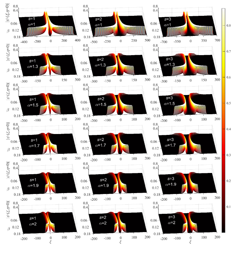
Figure 4: (Color online) Profiles of the cross-section, $\left|\psi\left(\xi,\eta=0\right)\right|$, of the vortex solitons for the propagation constant taking values $0.006\leq\beta\leq 0.18$ with an interval of $0.001$, and a set of different values of the vorticity and Lévy index, from $\alpha=1.0$ to $\alpha=2.0$, as indicated in the panels.

III.3 The linear-stability analysis and dynamics

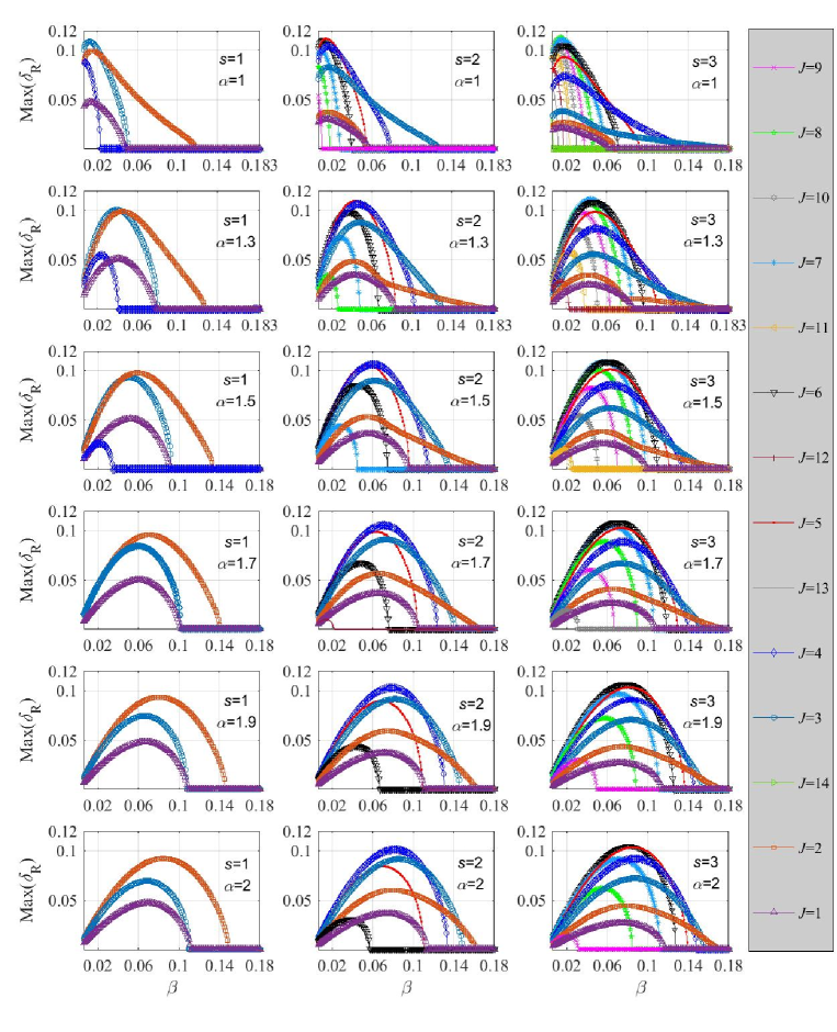
Figure 5: (Color online) The growth rate of perturbation eigenmodes with azimuthal indices $J$ versus the propagation constant $\beta$ of the underlying unperturbed vortex soliton, for different values of the Lévy index, from $\alpha=1.0$ to $\alpha=2.0$, as indicated in the panels.

As mentioned above, stability of VSs against the splitting instability is a crucially important issue. First, we address it in the framework of the linearization of Eq. (2) for small perturbations (i.e., the respective Bogoliubov-de Gennes equations), taking the perturbed solution as

$$\Psi\left(\xi,\eta,\zeta\right)=e^{i\beta\zeta}\left[\psi\left(\xi,\eta\right)+\epsilon u\left(\xi,\eta\right)e^{\delta\zeta}+\epsilon v^{\ast}\left(\xi,\eta\right)e^{\delta^{\ast}\zeta}\right],$$ (16)

where $\psi$ is the stationary VS solutions with propagation constant $\beta$, taken as per Eq. (5), while $u\left(\xi,\eta\right)$ and $v\left(\xi,\eta\right)$ represent eigenmodes of perturbations, with an infinitesimal amplitude $\epsilon$. In cylindrical coordinates $(r,\theta,\zeta)$, expression (16), including disturbances characterized by an integer azimuthal index, $J$, and instability growth rate, $\delta$ (which may be complex), is written as

$$\Psi\left(r,\theta,\zeta\right) = e^{i\left(\beta\zeta+s\theta\right)}\left[U\left(r\right)+\epsilon\varepsilon_{J}^{+}\left(r\right)e^{+iJ\theta}e^{\delta\zeta}\right.$$ (18)

$$\left.+\epsilon\varepsilon_{J}^{-}\left(r\right)e^{-iJ\theta}e^{\delta^{\ast}\zeta}\right],$$

where $\ast$ stands for the complex conjugate, while $\varepsilon_{J}^{+}\left(r\right)$ and $\varepsilon_{J}^{-}\left(r\right)$ are the respective perturbation eigenmodes.

Substituting Eq. (16) into Eq. (2) and the linearization lead to the following eigenvalue problem:

$$i\left(\begin{array}[]{cc}\mathcal{L}_{11}&\mathcal{L}_{12}\\ \mathcal{L}_{21}&\mathcal{L}_{22}\end{array}\right)\left(\begin{array}[]{c}u\\ v\end{array}\right)=\delta\left(\begin{array}[]{c}u\\ v\end{array}\right),$$ (19)

with matrix elements

$$\mathcal{L}_{11}=+\left[-\left(-\nabla_{\perp}^{2}\right)^{\alpha/2}+2\left|\psi\right|^{2}-3\left|\psi\right|^{4}-\beta\right],$$ (20)

$$\mathcal{L}_{12}=+\psi^{2}+2\left|\psi\right|^{2}\psi^{2},$$ (21)

$$\mathcal{L}_{21}=-\psi^{\ast 2}-2\left|\psi\right|^{2}\psi^{\ast 2},$$ (22)

$$\mathcal{L}_{22}=-\left[-\left(-\nabla_{\perp}^{2}\right)^{\alpha/2}+2\left|\psi\right|^{2}-3\left|\psi\right|^{4}-\beta\right]$$ (23)

where $\delta$ is a complex eigenvalue of Eq. (19). Obviously, stability demands to have only pure imaginary eigenvalues $\mu$.

The linear problem based on Eq. (19) can be solved by means of the Newton-conjugate-gradient method Book1 (written in the Cartesian coordinates), with the initial guess for the perturbation eigenmodes taken as per Eq. (18). Dependencies of the so found largest perturbation growth rates, $\delta_{\mathrm{R}}\equiv$Re$(\delta)$, on the propagation constant, for different values of $s$, $J$, and $\alpha$, are summarized in Fig. 5. It is seen that, for the unitary VS ($s=1$) at $\alpha=1.0$, $\alpha=1.3$, and $\alpha=1.5$, the azimuthal index of the dominant perturbation eigenmode switches from $J=3$ to $J=2$ with the increase of $\beta$, which is different from the case of the usual NLSE with $\alpha=2$. The decrease of the Lévy index also leads to switch of the azimuthal index of the dominant perturbation eigenmode for the VS solutions with $s=2$ and $3$. Especially, for the VS solutions with $s=2$ at $\alpha=1.0$, the perturbation eigenmode with the azimuthal index $J=2$ (it is one of the dominant perturbation eigenmodes for the VS solutions with $s=2$ ranging from $\alpha=1.3$ to $\alpha=2$) is suppressed, but, the azimuthal index $J=3$ becomes the dominant perturbation eigenmode with the increase of $\beta$. This lead to the stability area of the VSs with $s=2$ sharply shrinks for $\alpha=1$. Typical examples of perturbation eigenmodes $\varepsilon_{J}^{+}$ and $\varepsilon_{J}^{-}$ for the VSs with different values of $J$, are displayed in Fig. 6.

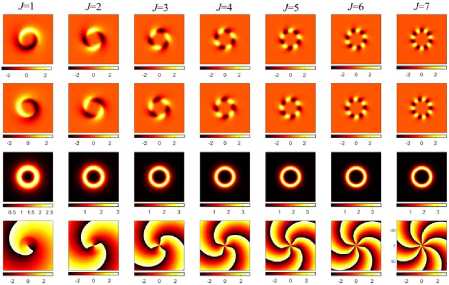
Figure 6: (Color online) Perturbation eigenmodes for the vortex soliton with $s=2$ and $\beta=2$, with Lévy index $\alpha=1.5$ and different values of the eigenmode’s azimuthal index, $J$. The first and second rows depict the real and imaginary parts of the eigenmodes, while the third and fourth rows show their intensity and phase patterns. In all panels, the displayed domain is $[-80,80]\times[-80,80]$.

The impact of the Lévy index on the stability area of the VSs, in which all eigenvalues $\delta$ are imaginary, is summarized in Table 1, while ${\beta}_{\,\min}{(s=3)}$ corresponds to the VSs with radii so large that it is difficult to find those values with sufficient accuracy.

To verify the validity of the results, the stability boundaries of the VS solutions in the usual NLSE with $\alpha=2$ was also recalculated by means of the numerical method adopted in this work, with a conclusion that the results are identical to those previously reported in Refs. CQ6b ; CQ12 . A noteworthy feature revealed by Table 1 is that the stability region of the unitary VS with $s=1$ shrinks with the decrease of the Lévy index from $\alpha=1$ up to $\alpha=2$, while, on the contrary, it expands for the VSs with $3$. It is worth noting that the stability area of the VSs with $s=2$ expands for $1<\alpha\leq 2$, but sharply shrinks for $\alpha=1$.

	$s$		$\alpha=1$	$\alpha=1.3$	$\alpha=1.5$	$\alpha=1.7$	$\alpha=1.9$	$\alpha=2$
	$1$		$0.119(1553)$	$0.128(532)$	$0.135(383)$	$0.141(285)$	$0.147(217)$	$0.149(199)$
	$2$		$0.127(3822)$	$0.178(32385)$	$0.170(6651)$	$0.165(1632)$	$0.163(761)$	$0.162(600)$
	$3$			$0.182(130586)$	$0.179(21546)$	$0.176(6112)$	$0.173(2113)$	$0.170(1364)$

Table 1: Vortex solitons are stable in intervals of the propagation constant $\beta_{\min}\leq\beta<\beta_{\max}\equiv 3/16$, with the lower boundary $\beta_{\min}$($P_{\min}$) shown in entries of the table, where $P_{\min}$ is the corresponding value of the power, for different values of vorticity $s$ and Lévy index $\alpha$.

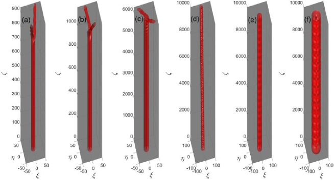
Figure 7: (Color online) Examples of the simulated evolution of the unitary vortex solitons with $s=1$ and propagation constant $\beta=0.14$, for different values of the Lévy index, $\alpha$. The evolution is displayed by isosurfaces drawn at the local intensity, $\left|\Psi\right|^{2}$, fixed at the half-maximum level. The evolution is unstable for $\alpha=2.0$ (a), $\alpha=1.9$ (b), and $\alpha=1.7$ (c). In panels (d), (e), and (f) stable evolutions are shown for $\alpha=1.5$, $\alpha=1.3$, and $\alpha=1.0$ under the action of random-noise perturbation at the $5\%$ amplitude level.

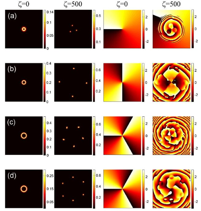
Figure 8: (Color online) Splitting of unstable vortex-soliton solutions at $\alpha=1.5$. The first and second columns show intensities of the input and output, while the third and last ones show the same for the corresponding phases. (a) The unitary vortex soliton, with $s=1$ and $\beta=0.03$. (b) The soliton with $s=2$ and $\beta=0.08$. (c) and (d): The solitons with $s=3$ and $\beta=$ $0.095$ and $\beta=0.06$, respectively. All panels are displayed in the domain of size $[-150,150]\times[-150,150]$.

Results predicted by the linear-stability analysis and collected in Fig. 5 and Table 1 were verified by direct simulations of the perturbed simulations of the VSs, performed in the framework of Eq. (2). First, the (in)stability of the unitary VS solutions with $s=1$ and fixed $\beta=0.14$ is tested for different values of the Lévy index. The simulations, displayed in Fig. 7, indicate that, in agreement with the predictions of the linear-stability analysis, in panels (a-c) the solutions are unstable against azimuthal perturbations, splitting into two fragments when the Lévy index takes values $\alpha=2$, $1.9$ and $1.7$. Further, the distance of stable propagation increases with the decrease of the Lévy index. Namely, at $\alpha=2$ ($\delta_{R}\approx 0.0373$), the splitting starts relatively fast in Fig. 7(a), at $\zeta\approx 800$, while, at $\alpha=1.9$ ($\delta_{R}\approx 0.0284$), it starts at $\zeta\approx 1000$ in Fig. 7(b). Further, at $\alpha=1.7$ the instability growth rate is very small, $\delta_{R}\approx 0.0041$, and, accordingly, the VS breaks only at $\zeta\approx 6100$ in Fig. 7(c). Finally, also in agreement with the linear-stability prediction, at $\alpha=1.5$, $\alpha=1.3$, and $\alpha=1.0$ the evolutions of the VSs are completely stable in Figs. 7(d), 7(e), and 7(f), even if it is perturbed by azimuthal random noise at the $5\%$ amplitude level, and the simulation is extremely long: the total propagation length, $\zeta=10000$, roughly corresponds to $100$ characteristic diffraction lengths of the beam. This length is estimated, in term of the beam’s width $W$, as $\zeta_{\mathrm{diffr}}\sim W^{\alpha}$. Additional long-scale simulations of the evolution of stable VSs under the action of noisy perturbations demonstrates slow random drift of the soliton’s center, and, in some cases, small deformation of the intensity ring. The increase of $\beta$, i.e., as a matter of fact, of the soliton’s total power, naturally leads to suppression of the drift and deformation. This dynamics is illustrated by movies in Supplemental Material SM1 .

Finally, in Fig. 8 we display additional results illustrating the development of splitting of unstable VSs, with vorticities $s=1,2$ and $3$. In all cases, it is concluded that the number of fragments (whose number grows from three to six with the increase of $s$) is determined by the fastest growing eigenmode of the azimuthal perturbations, in full agreement with the linear-stability analysis. Further details of the splitting dynamics are presented in movies included in Supplemental Material SM2 .

IV Conclusion

We have numerically investigated the existence and stability of families of spatial VS (vortex-soliton) solutions in the fractional NLSE with competing CQ (cubic-quintic) nonlinearities. A crucial difference from the usual two-dimensional NLSE, where there is no threshold for the existence of VS solutions, is that in the fractional model they exist at values of the soliton’s total power, $P$, exceeding a finite threshold. Accordingly, the dependence of the propagation constant on $P$ consists of two branches, which merge at $P=P_{\mathrm{thr}}$. Detailed results are reported for vorticities $s=1,2,$ and $3$.

The stability of the VS solutions has been investigated by means of the linearized equation for small perturbations. A remarkable conclusion is that the decrease of the Lévy index of the fractional NLSE leads to shrinkage of the stability area of the unitary ($s=1$) VS solutions, on the contrary, it expands for the solitons with $3$, especially, the stability area of the VSs with $s=2$ expands for $1<\alpha\leq 2$ but shrinks for $\alpha=1$. The predictions of the linear-stability analysis are fully corroborated by direct simulations, which, in particular, demonstrate splitting of unstable VSs in sets of fragments the number of which is exactly predicted by the dominant eigenmode of small perturbations.

As an extension of the present work, it may be interesting to address motion and collisions of stable VSs (note that the fractional NLSE is not a Galilean invariant one, therefore the mobility of solitons is a nontrivial issue).

V Acknowledgments

This work was supported by the National Natural Science Foundation of China (NNSFC) (11805141, 11804246) and Shanxi Province Science Foundation for Youths (201901D211424), and supported by Scientific and Technological Innovation Programs of Higher Education Institutions in Shanxi (STIP) (2019L0782). The work of BAM was supported, in a part, by the Israel Science Foundation through grant No. 1286/17.

References

- (1) Trillo S, Torrellas W, editors. Spatial Solitons. Berlin: Springer; 2001.
- (2) Staliunas K, Sánchez-Morcillo VJ. Transverse Patterns in Nonlinear Optical Resonators. Berlin: Springer; 2002.
- (3) Rosanov NN. Spatial Hysteresis and Optical Patterns. Berlin: Springer; 2002.
- (4) Kivshar Y, Agrawal G. Optical Solitons. San Diego: Academic; 2003.
- (5) Lederer F, Stegeman GI, Christodoulides DN, Assanto G, Segev M, Silberberg Y. Discrete solitons in optics. Phys Rep 2008;463(1-3):1-126.
- (6) Ackemann T, Firth WJ, Oppo GL. Fundamentals and applications of spatial dissipative solitons in photonic devices. Adv At Mol Opt Phys 2009;57:324-421.
- (7) Kartashov YV, Vysloukh VA, Torner L. Soliton shape and mobility control in optical lattices. Prog Optics 2009;52:63-148.
- (8) Yang JK. Nonlinear waves in integrable and nonintegrable systems. Philadelphia:SIAM; 2010.
- (9) Peccianti M, Assanto G. Nematicons. Phys Rep 2012;516(4):147-208.
- (10) Chen Z, Segev M, Christodoulides DN. Optical spatial solitons: historical overview and recent advances. Rep Prog Phys 2012;75(8):086401.
- (11) Konotop VV, Yang JK, Zezyulin DA. Nonlinear waves in -symmetric systems. Rev Mod Phys 2016;88(3):035002.
- (12) Tlidi M, Panajotov K. Cavity solitons: Dissipative structures in nonlinear photonics. Rom Rep Phys 2018;70(1):406.
- (13) Rosanov NN, Fedorov SV, Veretenov NA. Laser solitons in 1D, 2D and 3D. Eur Phys J D 2019;73(7):141.
- (14) Lund F, Regge T. Unified approach to strings and vortices with soliton solutions. Phys Rev D 1976;14(6-15):1524-1535.
- (15) Kovalev AS, Kosevich AM, Maslov KV. Magnetic vortex – topological soliton in a ferromagnet with an easy-axis anisotropy. JETP Lett 1979;30:296-299.
- (16) Ezawa ZF. Local field theories for vortex solitons. Phys Lett B 1979;82(3-4):426-430.
- (17) Nozaki K. Vortex solitons of drift waves and anomalous diffusion. Phys Rev Lett 1981;46(3-19):184-187.
- (18) Kundu A, Rybakov YP. Cosed-vortex-type solitons with Hopf index. J Math A: Math Gen 1982;15(1):269-275.
- (19) Kruglov VI, Vlasov RA. Spiral self-trapping propagation of optical beams in media with cubic nonlinearity. Phys Lett A 1985(8-9);111:401-404.
- (20) Nevzlin MV, Rossby solitons (Experimental investigations and laboratory model of natural vortices of the Jovian Great Red Spot type), Sov Phys Usp 1986;29(9):807-842.
- (21) Desyatnikov A, Kivshar Y, Torner L. Optical vortices and vortex solitons. Prog Opt 2005;47:291-391.
- (22) Malomed BA, Mihalache D, Wise F, Torner L. Spatiotemporal optical solitons. J Optics B: Quant Semicl Opt 2005;7(5):R53-R72.
- (23) Radu E, Volkov MS. Stationary ring solitons in field theory – Knots and vortons. Phys Rep 2008;468(4):101-151.
- (24) Malomed BA. Multidimensional solitons: Well-established results and novel findings. Eur Phys J Special Topics 2016;225:2507-2532.
- (25) Mihalache D. Multidimensional localized structures in optical and matter-wave media: a topical survey of recent literature. Rom Rep Phys 2017;69(1):403.
- (26) Kartashov YV, Astrakharchik GE, Malomed BA, Torner L. Frontiers in multidimensional self-trapping of nonlinear fields and matter. Nat Rev Phys 2019;1:185-197.
- (27) Malomed BA. (INVITED) Vortex solitons: Old results and new perspectives. Physica D 2019;399:108-137.
- (28) Malomed BA, Mihalache D. Nonlinear waves in optical and matter-wave media: A topical survey of recent theoretical and experimental results. Rom J Phys 2019;64(5-6):106.
- (29) Chiao RY, Garmire E, Townes CH. Self-trapping of optical beams. Phys Rev Lett 1964;13(15):479.
- (30) Torner L, Petrov DV. Azimuthal instabilities and self-breaking of beams into sets of solitons in bulk secondharmonic generation. Electron Lett 1997;33(7):608-610.
- (31) Firth WJ, Skryabin DV. Optical Solitons Carrying Orbital Angular Momentum. Phys Rev Lett 1997;79(13):2450-2453.
- (32) Towers I, Buryak AV, Sammut RA, Malomed BA. Stable localized vortex solitons. Phys Rev E 2000;63(5):055601(R).
- (33) Mihalache D, Mazilu D, Crasovan LC, Towers I, Malomed BA, Buryak AV, Torner L, Lederer F. Stable three-dimensional spinning optical solitons supported by competing quadratic and cubic nonlinearities. Phys Rev E 2002;66(1):016613.
- (34) Mihalache D, Mazilu D, Malomed BA, Lederer F. Stable vortex solitons supported by competing quadratic and cubic nonlinearities. Phys Rev E 2004;69(6):066614.
- (35) Quiroga-Teixeiro ML, Michinel H. Stable azimuthal stationary state in quintic nonlinear optical media. J Opt Soc Am B 1997;14(8):2004-2009.
- (36) Quiroga-Teixeiro ML, Berntson A, Michinel H. Internal dynamics of nonlinear beams in their ground states: short- and long-lived excitation. J Opt Soc Am B 1999;16(10):1697-1704.
- (37) Desyatnikov A, Maimistov A, Malomed BA. Three-dimensional spinning solitons in dispersive media with the cubic-quintic nonlinearity. Phys Rev E 2000;61(3):3107-3113.
- (38) Mihalache D, Mazilu D, Crasovan LC, Malomed BA, Lederer F. Three-dimensional spinning solitons in the cubic-quintic nonlinear medium. Phys Rev E 2000;61(6):7142-7145.
- (39) Malomed BA, Crasovan LC, Mihalache D. Stability of vortex solitons in the cubic-quintic model. Physica D 2002;161(3-4):187-201.
- (40) Towers I, Buryak AV, Sammut RA, Malomed BA, Crasovan LC, Mihalache D. Stability of spinning ring solitons of the cubic-quintic nonlinear Schrödinger equation. Phys Lett A 2001;288(5-6):292-298.
- (41) Michinel H, Campo-Táboas J, Quiroga-Teixeiro ML, Salgueiro JR, García-Fernández R. Excitation of stable vortex solitons in nonlinear cubic-quintic materials. J Opt B: Quantum Semiclass Opt. 2001;3(5):314-317.
- (42) Crasovan LC, Malomed BA, Mihalache D. Spinning solitons in cubic-quintic nonlinear media. Pramana-J Phys 2001;57(5-6):1041-1059.
- (43) Pego RL, Warchall HA. Spectrally stable encapsulated vortices for nonlinear Schrödinger equations. J Nonlinear Sci 2002;12(4):347-394.
- (44) Mihalache D, Mazilu D, Towers I, Malomed BA, Lederer F. Stable two-dimensional spinning solitons in a bimodal cubic-quintic model with four-wave mixing. J Opt A: Pure Appl Opt 2002;4(6):615-623.
- (45) Mihalache D, Mazilu D, Crasovan LC, Towers I, Buryak AV, Malomed BA, Torner L, Torres JP, Lederer F. Stable spinning optical solitons in three dimensions. Phys Rev Lett 2002;88(7):073902.
- (46) Mihalache D, Mazilu D, Towers I, Malomed BA, Lederer F. Stable spatiotemporal spinning solitons in a bimodal cubic-quintic medium. Phys Rev E 2003;67(5):056608.
- (47) Dong LW, Ye FW, Wang JD, Cai T, Li YP. Internal modes of localized optical vortex soliton in a cubic-quintic nonlinear medium. Physica D 2004;194(3-4):219-226.
- (48) Dror N, Malomed BA. Symmetric and asymmetric solitons and vortices in linearly coupled two-dimensional waveguides with the cubic-quintic nonlinearity. Physica D 2011;240(6):526-541.
- (49) Caplan RM, Carretero-González R, Kevrekidis PG, Malomed BA. Existence, stability, and scattering of bright vortices in the cubic-quintic nonlinear Schrödinger equation. Math Comp Simul 2012;82(7):1150-1171.
- (50) Yakimenko AI, Zaliznyak YA, Kivshar Y. Stable vortex solitons in nonlocal self-focusing nonlinear media. Phys Rev E 2005;71(6):065603(R).
- (51) Briedis D, Petersen DE, Edmundson D, Krolikowski W, Bang O. Multipole spatial vector solitons. Opt Exp 2005;13(2):435-437.
- (52) Ye FW, Kartashov YV, Hu B, Torner L. Twin-vortex solitons in nonlocal nonlinear media. Opt Lett 2010;35(5):628-630.
- (53) Assanto G, Minzoni AA, Smyth NF. Deflection of nematicon-vortex vector solitons in liquid crystals. Phys Rev A 2014;89(1):013827.
- (54) Assanto G, Minzoni AA, Smyth NF. Vortex confinement and bending with nonlocal solitons. Opt Lett 2014;39(3):509-512.
- (55) Izdebskaya Y, Assanto G, Krolikowski W. Observation of stable-vector vortex solitons. Opt Lett 2015;40(17):4182-4185.
- (56) Zhang H, Chen M, Yang L, Tian B, Chen C, Guo Q, Shou Q, Hu W. Higher-charge vortex solitons and vector vortex solitons in strongly nonlocal media. Opt Lett 2019;44(12):3098-3101.
- (57) Pushkarov KI, Pushkarov DI, Tomov IV. Self-action of light beams in nonlinear media: soliton solutions. Opt Quantum Electron 1979;11(6):471-478.
- (58) Hu Y, Kallianpur G. Schrödinger Equations with Fractional Laplacians. Appl Math Optim 2000;42(3):281-290.
- (59) Laskin N. Fractional Schrödinger equation. Phys Rev E 2002;66(5):056108.
- (60) Laskin N. Fractional quantum mechanics. Phys Rev E 2000;62(3):3135-3145.
- (61) Laskin N. Fractional quantum mechanics and Lévy path integrals. Phys Lett A 2000;268(4-6):298-305.
- (62) Wei YC. Comment on “Fractional quantum mechanics” and “Fractional Schrödinger equation”. Phys Rev E 2016;93(6):066103.
- (63) Laskin N. Reply to “Comment on ‘Fractional quantum mechanics’ and ‘Fractional Schrödinger equation’”. Phys Rev E 2016;93(6):066104.
- (64) Stickler BA. Potential condensed-matter realization of space-fractional quantum mechanics: The one-dimensional Lévy crystal. Phys Rev E 2013;88(1):012120.
- (65) Longhi S. Fractional Schrödinger equation in optics. Opt Lett 2015;40(6):1117-1120.
- (66) Zhang YQ, Liu X, Belić MR, Zhong WP, Zhang YP, Xiao M. Propagation dynamics of a light beam in a fractional Schrödinger equation. Phys Rev Lett 2015;115(18):180403.
- (67) Zhang YQ, Zhong H, Belić MR, Ahmed N, Zhang YP, Xiao M. Diffraction-free beams in fractional Schrödinger equation. Sci Rep 2016;6(1):23645.
- (68) Huang XW, Deng ZX, Fu XQ. Diffraction-free beams in fractional Schrödinger equation with a linear potential. J Opt Soc Am B 2017;34(5):976-982.
- (69) Huang XW, Deng ZX, Shi XH, Fu XQ. Propagation characteristics of ring Airy beams modeled by the fractional Schrödinger equation. J Opt Soc Am B 2017;34(10):2190-2197.
- (70) Huang XW, Deng ZX, Bai YF, Fu XQ. Potential barrier-induced dynamics of finite energy Airy beams in fractional Schrödinger equation. Opt Exp 2017;25(26):32560-32569.
- (71) Zhang D, Zhang YQ, Zhang ZY, Ahmed N, Zhang YP, Li FL, Belić MR, Xiao M. Unveiling the link between fractional Schrödinger equation and light propagation in honeycomb lattice. Ann Phys (Berlin) 2017;529(9):1700149.
- (72) Zhang LF, Li CX, Zhong HZ, Xu CW, Lei DL, Li Y, Fan DY. Propagation dynamics of super-Gaussian beams in fractional Schrödinger equation: from linear to nonlinear regimes. Opt Exp 2016;24(13):14406-14418.
- (73) Zang F, Wang Y, Li L. Dynamics of Gaussian beam modeled by fractional Schrödinger equation with a variable coefficient. Opt Exp 2018;26(18):23740-23750.
- (74) Huang CM, Dong LW. Beam propagation management in a fractional Schrödinger equation. Sci Rep 2017;7(1):5442.
- (75) Zhang YQ, Wang R, Zhong H, Zhang JW, Belić MR, Zhang YP. Optical Bloch oscillation and Zener tunneling in the fractional Schrödinger equation. Sci Rep 2017;7(1):17872.
- (76) Zhang YQ, Wang R, Zhong H, Zhang JW, Belić MR, Zhang YP. Resonant mode conversions and Rabi oscillations in a fractional Schrödinger equation. Opt Exp 2017;25(26):32401-32410.
- (77) Huang CM, Shang C, Li J, Dong LW, Ye FW. Localization and Anderson delocalization of light in fractional dimensions with a quasi-periodic lattice. Opt Exp 2019;27(5):6259-6267.
- (78) Li PF, Li JD, Han BC, Ma HF, Mihalache D. PT-symmetric optical modes and spontaneous symmetry breaking in the space-fractional Schrödinger equation. Rom Rep Phys 2019;71(2):106.
- (79) Fujioka J, Espinosa A, Rodríguez RF. Fractional optical solitons. Phys Lett A 2010;374(9):1126-1134.
- (80) Klein C, Sparber C, Markowich P. Numerical study of fractional nonlinear Schrödinger equations. Proc R Soc A 2014;470(2172):20140364.
- (81) Borovkova OV, Lobanov VE, Malomed BA. Solitons supported by singular spatial modulation of the Kerr nonlinearity. Phys Rev A 2012;85(2):023845.
- (82) Chen MN, Zeng SH, Lu DQ, Hu W, Guo Q. Optical solitons, self-focusing, and wave collapse in a space-fractional Schrödinger equation with a Kerr-type nonlinearity. Phys Rev E 2018;98(2):022211.
- (83) Zhong WP, Belić MR, Zhang YQ. Accessiblesolitons of fractional dimension. Ann Phys 2016;368:110-116.
- (84) Zhong WP, Belić MR, Malomed BA, Zhang YQ, Huang TW. Spatiotemporal accessible solitons in fractional dimensions. Phys Rev E 2016;94(1):012216.
- (85) Zhong WP, Belić MR, Zhang YQ. Fractional dimensional accessible solitons in a parity-time symmetric potential. Ann Phys (Berlin) 2018;530(2):1700311.
- (86) Dong LW, Huang CM. Double-hump solitons in fractional dimensions with a PT-symmetric potential. Opt Express 2018;26(8):10509.
- (87) Huang CM, Deng HY, Zhang WF, Ye FW, Dong LW. Fundamental solitons in the nonlinear fractional Schrödinger equation with a PT-symmetric potential. Europhys Lett 2018;122(2):24002.
- (88) Huang CM, Dong LW. Gap solitons in the nonlinear fractional Schrödinger equation with an optical lattice. Opt Lett 2016;41(24):5636-5639.
- (89) Xiao J, Tian ZX, Huang CM, Dong LW. Surface gap solitons in a nonlinear fractional Schrödinger equation. Opt Exp 2018;26(3):2650-2658.
- (90) Zhu X, Yang FW, Cao SL, Xie JQ, He YJ. Multipole gap solitons in fractional Schrödinger equation with parity-time-symmetric optical lattices. Opt Exp 2020;28(2):1631-1639.
- (91) Dong LW, Huang CM. Vortex solitons in fractional systems with partially parity-time-symmetric azimuthal potentials. Nonl. Dyn. 2019;98(8):1019-1028.
- (92) Yao XK, Liu XM. Solitons in the fractional Schrödinger equation with parity-time-symmetric lattice potential. Photonics Res 2018;6(9):875-879.
- (93) Li P, Malomed BA, Mihalache D. Symmetry breaking of spatial Kerr solitons in fractional dimension, Chaos Solitons Fract 2020;132:109602.
- (94) Qiu Y, Malomed BA, Mihalache D, Zhu X, Zhang L, He YJ, Soliton dynamics in a fractional complex Ginzburg-Landau model, Chaos Solitons Fract 2020; in press.
- (95) Huang CM, Dong LW. Composition relation between nonlinear Bloch waves and gap solitons in periodic fractional systems. Materials 2018;11(7):1134.
- (96) Zeng LW, Zeng JH. One-dimensional gap solitons in quintic and cubic-quintic fractional nonlinear Schrödinger equations with a periodically modulated linear potential. Nonlinear Dyn. 2019;98:985-995.
- (97) Zeng LW, Zeng JH. One-dimensional solitons in fractional Schrödinger equation with a spatially periodical modulated nonlinearity: nonlinear lattice. Opt Lett 2019;44(11):2661-2664.
- (98) Huang CM, Dong LW. Dissipative surface solitons in a nonlinear fractional Schrödinger equation. Opt Lett 2019;44(22):5438-5441.
- (99) Molina MI. The fractional discrete nonlinear Schrödinger equation. Phys Lett A 2020;384(8):126180.
- (100) Yao XK, Liu XM. Off-site and on-site vortex solitons in space-fractional photonic lattices. Opt Lett 2018;43(23):5749-5752.
- (101) Jeng M, Xu SLY, Hawkins E, Schwarz JM. On the nonlocality of the fractional Schrödinger equation. J Math Phys 2010;51(6):062102.
- (102) Luchko Y. Fractional Schrödinger equation for a particle moving in a potential well. J Math Phys 2013;54(1):012111.
- (103) Duo SW, Zhang YZ. Mass-conservative Fourier spectral methods for solving the fractional nonlinear Schrödinger equation. Comput Math Appl 2016;71(11):2257-2271.
- (104) Yang JK. Newton-conjugate-gradient methods for solitary wave computations. J Comput Phys 2009;228(18):7007-7024.
- (105) Vakhitov NG, Kolokolov SA. Stationary solutions of the wave equation in a medium with nonlinearity saturation. Radiophys Quantum Electron 1973;16(7):783-789.
- (106) Fibich G. The Nonlinear Schrödinger Equation: Singular Solutions and Optical Collapse. Heidelberg: Springer; 2015.
- (107) Birnbaum Z, Malomed BA. Families of spatial solitons in a two-channel waveguide with the cubic-quintic nonlinearity. Physica D 2008;237(24):3252-3262.
- (108) See Supplemental Materials for Fig. S1a.avi (, , ), Fig. S1b.avi (, , ), Fig. S1c.avi (, , ), and Fig. S1d.avi (, , ).
- (109) See Supplemental Materials for Fig.S2a.avi, Fig.S2b.avi, Fig. S2c.avi, and Fig. S2d.avi.